Wavefront’s stability with asymptotic phase in the delayed monostable equations

Abstract.

We extend the class of initial conditions for scalar delayed reaction-diffusion equations $u_{t}(t,x)=u_{xx}(t,x)+f(u(t,x),u(t-h,x))$ which evolve in solutions converging to monostable traveling waves. Our approach allows to compute, in the moving reference frame, the phase distortion $\alpha$ of the limiting travelling wave with respect to the position of solution at the initial moment $t=0$. In general, $\alpha\not=0$ for the Mackey-Glass type diffusive equation. Nevertheless, $\alpha=0$ for the KPP-Fisher delayed equation: the related theorem also improves existing stability conditions for this model.

1. Introduction: main results and applications

The previous studies (e.g. see [2, 3, 10, 14]) show that both minimal and non-minimal positive traveling waves $u(t,x)=\phi(x+ct)$ for the monostable delayed reaction-diffusion equation

(1.1) $$u_{t}(t,x)=u_{xx}(t,x)+f(u(t,x),u(t-h,x)),\quad t>0,\ x\in{\mathbb{R}},$$

attract solutions $u(t,x)$ whose initial segments $u_{0}(s,x)$ have the same leading asymptotic terms at $x=-\infty$ as the shifted wave $\phi(x+cs)$, for all $s\in[-h,0]$. The latter assumption implies that, for some positive $A_{0}$,

(1.2) $$\lim_{x\to-\infty}\frac{u_{0}(s,x)}{\phi(x+cs)}=A_{0},\quad s\in[-h,0].$$

This observation concerns so-called pulled waves for equation (1.1) and smooth traveling waves for delayed degenerate reaction-diffusion equations [8]. The pushed and bistable waves have better stability properties [11, 12] and they are not considered in this work.

Condition (1.2) seems to be excessively restrictive: for example, it excludes initial segments asymptotically similar, in the spirit of (1.2), to $\phi(x+\alpha(s)),$ $s\in[-h,0]$, with nonlinear shift $\alpha(s)$. This circumstance is irrelevant for the non-delayed equations when $h=0$, however, in the delayed case it restricts severely the range of possible applications. Analysing this problem, in [11, Corollary 1] we have shown, under a quasi-monotonicity condition on $f$, that the existence of the limit

(1.3) $$\lim_{x\to-\infty}\frac{u_{0}(s,x)}{\phi(x+cs)}=A_{0}(s)>0,\quad s\in[-h,0],$$

with some continuous function $A_{0}(s)$ implies that solution $u(t,x)$ evolves in the middle of two shifted traveling waves constituting the lower bound $u_{-}(t,x)=\phi(x+ct+a_{-}),$ and the upper bound $u_{+}(t,x)=\phi(x+ct+a_{+})$. Condition (1.3) is easily verifiable. Indeed, it is well known that under some natural restrictions (tacitly assumed in this work) so-called non-critical waves have the following asymptotic representation after an appropriate translation of the time variable:

(1.4) $$\phi(t) = e^{\lambda_{1}t}+e^{(\lambda_{1}+\sigma)t}r_{1}(t),\ \lambda_{1}+\sigma<\lambda_{2},$$

$$\phi^{\prime}(t) = \lambda_{1}e^{\lambda_{1}t}+e^{(\lambda_{1}+\sigma)t}r_{2}(t),\quad\quad t\in{\mathbb{R}}.$$

Here $\sigma$ is a positive number, $r_{1},\,r_{2}$ are smooth bounded functions and $0<\lambda_{1}<\lambda_{2}$ are zeros of the characteristic function $\chi_{0}(z)=z^{2}-cz+f_{1}(0,0)+f_{2}(0,0)e^{-zch}$. In the paper, $f_{j}(u,v)$ denotes the partial derivative of $f$ with respect to $j$-th argument. We will assume that $f_{j}(u,v)$ are locally Lipschitz continuous functions.

A potential possibility that solution $u(t,x)$ can develop non-decaying oscillations between the waves $u_{+}(t,x)$ and $u_{-}(t,x)$ was not discarded in [11]. Another question left open in [11] is whether such $u(t,x)$ converges to the traveling wave in form and in speed [9, 13], i.e. whether there exists a function $\beta(t)$ such that $\beta(t)/t\to c$ and $u(t,x-\beta(t))\to\phi(x)$ as $t\to+\infty$, uniformly on subsets $(-\infty,n],$ $n\in{\mathbb{N}}$. In this work, we answer both questions under rather realistic assumptions specified below.

Actually, assuming (1.3), we prove that the solution $u(t,x)$ converges to a shifted wave $\phi(x+ct+a_{*})$, where $a_{*}$ is completely determined by the function $A_{0}(s)$:

(1.5) $$a_{*}=\frac{1}{\lambda_{1}}\ln A_{\infty},\quad\mbox{where}\ A_{\infty}:=\frac{A_{0}(0)+q\int_{-h}^{0}A_{0}(s)ds}{1+qh},\ q:=\frac{f_{2}(0,0)e^{-\lambda_{1}ch}}{\lambda_{1}}.$$

We obtain $A_{\infty}$ as the limit value at $+\infty$ of the solution $A(t),\ t\geq 0$, to the initial value problem $A(s)=A_{0}(s)>0,$ $s\in[-h,0]$, for the monotone scalar delay differential equation

(1.6) $$A^{\prime}(t) = q\left(A(t-h)-A(t)\right),\quad\quad t\geq 0.$$

Indeed, it is clear that $A(t)>0$ for all $t\geq-h$. Since the characteristic equation $z+q=qe^{-zh}$ for equation (1.6) with $f_{2}(0,0)>0$ has a unique simple real root $z=0$, other (complex) roots $z_{j}$ satisfying the inequality ${\mathbb{R}}e\,z_{j}<0$ (see Appendix), there are real numbers $A_{\infty}\geq 0$ and $d<0$ (cf. [1, Theorem 3.2]) such that

(1.7) $$|A(t)-A_{\infty}|\leq e^{dt},\quad t\geq 0.$$

By integrating (1.6) on ${\mathbb{R}}_{+}$, we find that

$$A_{\infty}(1+qh)=A_{0}(0)+q\int_{-h}^{0}A_{0}(s)ds>0.$$

Now, (1.3), (1.4) imply that the initial function $u(s,x)$ evaluated at the moment $s=0$ behaves as $\phi(x+a_{0}),$ where $a_{0}=\ln A_{0}(0)/\lambda_{1}$. Therefore the total traveled distance $\delta_{a}$ between the initial (at the moment $t=0$) and final (as $t\to+\infty$) positions of the solution in the moving reference frame is

$$\delta_{a}=a_{*}-a_{0}=\frac{1}{\lambda_{1}}\ln\frac{1+q\int_{-h}^{0}A_{0}(s)/A_{0}(0)ds}{1+qh}.$$

Note that the function $A(t)$ and $\delta_{a}$ are completely determined by the speed $c$, the initial values $A_{0}(s)$ and the partial derivatives $f_{1}(0,0),f_{2}(0,0)$. They do not depend on other characteristics of solution $u(t,x)$ and wavefront $\phi(x+ct)$, including their bounds $M_{1}\leq M_{3}\in{\mathbb{R}}\cup\{+\infty\},$ $M_{2}\leq 0$,

$$0\leq\phi(x)\leq M_{1},\quad M_{2}\leq u(t,x)\leq M_{3},\qquad(t,x)\in[-h,+\infty)\times{\mathbb{R}},$$

and associated parameters $L_{2}\geq f_{2}(0,0)\geq 0$ and $D\in{\mathbb{R}}$ chosen to satisfy

$$|f(w,v_{1})-f(w,v_{2})|\leq L_{2}\,|v_{1}-v_{2}|,\quad\quad(w,v_{1},v_{2})\in[0,M_{1}]\times[M_{2},M_{3}]^{2},$$

$$D=\inf_{(w_{1},w_{2},v)\in[M_{2},M_{3}]^{3},w_{1}\not=w_{2}}\frac{f(w_{1},v)-f(w_{2},v)}{w_{2}-w_{1}}.$$

Remark 1.1.

Clearly, $D=1$ for the Mackey-Glass type nonlinearity $f(w,v)=-w+b(v)$. Considering monotone wavefronts for the KPP-Fisher delayed equation [2, 4, 5, 6], when $f(w,v)=w(1-v)$, we find that $L_{2}=M_{1}=1$, $M_{3}=+\infty$. In the general case of non-monotone waves for the latter equation, we can take $L_{2}=M_{1}=e^{ch}$, $M_{3}=+\infty$, cf. [2]. In both cases (monote and non-monotone), we have that $D=\inf_{(t,x)\in[0,+\infty)\times{\mathbb{R}}}u(t,x)-1.$ Hence, if $u_{0}\geq 0=M_{2}$ then $D=-1$.

First, we consider an easier situation when $f_{2}(0,0)>0$.

Theorem 1.2.

Assume that $f_{2}(0,0)>0$ and

(1.8) $$\lambda^{2}-c\lambda-D-\gamma+L_{2}e^{-\lambda ch}e^{-\gamma h}<0,$$

for some $\lambda\in(\lambda_{1},\min\{2\lambda_{1},\lambda_{2}\})$ and $\gamma\in(d,0)$. If, in addition, $u_{0}(s,x)$ verifies

(1.9) $$|u_{0}(s,x)-\phi(x+cs+\alpha_{0}(s))|\leq Ke^{\lambda x},\qquad(s,x)\in[-h,0]\times{\mathbb{R}},$$

then, for some $K^{\prime}\geq K$, solution $u(t,x)$ of (1.1) with the initial function $u_{0}$ satisfies

(1.10) $$\sup_{x\in{\mathbb{R}}}\left(e^{-\lambda x}|u(t,x-ct-\alpha(t))-\phi(x)|\right)\leq K^{\prime}e^{\gamma t},\quad t\geq-h.$$

Here $A(t)=e^{\lambda_{1}\alpha(t)}$ solves (1.6) with the initial datum $A_{0}(s)=e^{\lambda_{1}\alpha_{0}(s)},$ $s\in[-h,0]$ so that $\alpha(+\infty)=a_{*}\in[\min_{[-h,0]}\alpha_{0}(s),\max_{[-h,0]}\alpha_{0}(s)]$ is given by (1.5). Finally, $\delta_{a}=0$ if and only if $A(0)=(1/h)\int_{-h}^{0}A_{0}(s)ds$.

Next, we consider the ‘degenerate’ situation when $f_{2}(0,0)=0$. From (1.6), we can expect that $\alpha(t)\equiv\alpha(0)$ for $t\geq 0$. Below, we prove that this is indeed the case for a class of the KPP-Fisher type nonlinearities.

Theorem 1.3.

Assume that $f(u,v)=g(u)(\kappa-v)$ with $\kappa>0$, $g(0)=0$, that (1.8) holds for some $\lambda\in(\lambda_{1},\lambda_{2})$ and $\gamma<0$, and that $u_{0}(s,x)$ satisfies, for some $\lambda^{*}>\lambda_{1}$,

(1.11) $$|u_{0}(s,x)-\phi(x+cs+\alpha_{0}(s))|\leq Ke^{\lambda^{*}x},\qquad(s,x)\in[-h,0]\times{\mathbb{R}}.$$

Set $\lambda_{*}=\min\{\lambda^{*},\lambda,2\lambda_{1}\}$. If $\lambda_{*}^{2}-c\lambda_{*}-D-\gamma<0$, then, for some $K^{\prime}\geq K$, solution $u(t,x)$ of equation (1.1) with the initial function $u_{0}(s,x)$ satisfies

(1.12) $$\sup_{x\in{\mathbb{R}}}\left(e^{-\lambda_{*}x}|u(t,x-ct-\alpha_{0}(0))-\phi(x)|\right)\leq K^{\prime}e^{\gamma t},\quad t\geq-h.$$

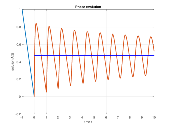
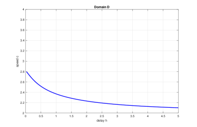
Figure 1. On the left: particular solution of (1.6) with $h=1$, $q=19$, $A_{0}(s)=-s$. Horizontal line is the limit value $A_{\infty}=19/40$. On the right, the graph of $c=c_{\#}(h)$ from Corollary 1.5.

Theorems 1.2 and 1.3 say that the evolution of the initial phase deviation $\alpha_{0}(s)$ is determined by the linear delay differential equation (1.6). More detailed analysis of the eigenvalues $z_{j}$ to (1.6) (see the Appendix) allows to have a better idea about the character of convergence of $\alpha(t)$ to its limit $\alpha(+\infty)$. We claim that, in the non-degenerate case $hf_{2}(0,0)\not=0$, $\alpha_{0}(s)\not\equiv const$, generically $\alpha(t)$ develops ‘rapid’ oscillations around $\alpha(+\infty)$ (these oscillations can be significant when $q$ is relatively large, see Figure 1). More precisely, generically $\alpha(t)$ crosses two times the level $\alpha(+\infty)$ on each half-open interval of the length $h$. Indeed, an application of the Laplace transform to (1.6) yields the following representation

$$A(t)=A_{\infty}+2\real(A_{1}e^{z_{1}t})(1+o(1)),\ \mbox{where}$$

$$A_{1}(1+h(z_{1}+q))=A_{0}(0)+qe^{-z_{1}h}\int_{-h}^{0}e^{-z_{1}s}A_{0}(s)ds$$

with $z_{1}=x_{1}+iy_{1},y_{1}h\in(\pi,2\pi)$, being the leading complex eigenvalue of (1.6).

In particular, $\alpha(t)$ is typically oscillating in the case of Nicholson’s diffusive equation [3, 10, 11, 14]

(1.13) $$u_{t}(t,x)=u_{xx}(t,x)-u(t,x)+b(u(t-h,x)),\ \ x\in{\mathbb{R}},\quad b(u)=pue^{-u},\ p>1,$$

In such a case, $L_{2}=b^{\prime}(0)=p$, $D=1$, and the solution $u(t,x),$ $t\geq 0,x\in{\mathbb{R}},$ is bounded once its initial fragment $u_{0}(s,x)$, $s\in[-h,0],x\in{\mathbb{R}},$ is bounded. In addition, the formulae (1.4) hold for each $c>c_{*}$, where $c_{*}$ is the minimal speed of propagation in the model. In this way, we obtain the following conclusion:

Corollary 1.4.

Let $u=\phi(x+ct)$ be a non-critical wave for the Nicholson’s diffusive equation. Denote by $u(t,x)$ solution of the initial problem $u(s,x)=u_{0}(s,x),$ $s\in[-h,0],$ for (1.13) where non-negative function $u_{0}$ satisfies

(1.14) $$|u_{0}(s,x)-\phi(x+cs+\alpha_{0}(s))|\leq Ke^{\lambda x},\qquad(s,x)\in[-h,0]\times{\mathbb{R}},$$

for some $\lambda>\lambda_{1}$. Then there exist $\mu\in(\lambda_{1},\lambda]$, $\gamma<0$ and $Q\geq K$ such that

$$|u(t,x)-\phi(x+ct+\alpha(t))|\leq Qe^{\mu(x+ct)}e^{\gamma t},\quad x\in{\mathbb{R}},\ t\geq-h.$$

The function $\alpha(t)$ is converging at $+\infty$ and generically develops ‘rapid’ oscillations around its limiting value $\alpha(+\infty)$.

Other aforementioned model, the KPP-Fisher delayed equation

(1.15) $$u_{t}(t,x)=u_{xx}(t,x)+u(t,x)(1-u(t-h,x)),\ u=u_{0}(s,x),s\in[-h,0],\ x\in{\mathbb{R}},$$

has the reaction term satisfying the equality $f_{2}(0,0)=0$. In view of Theorem 1.3 and Remark 1.1, in the general case of non-monotone waves we have to consider the domain ${\mathcal{D}}$ (presented on the right panel of Fig. 1 as a strict epigraph for the decreasing function $c=c_{\#}(h),\$ $h\geq 0,$ $\ c_{\#}(0)=2\sqrt{2},\ c_{\#}(+\infty)=2$),

$${\mathcal{D}}=\left\{(h,c):\lambda^{2}-c\lambda+1+e^{-\lambda ch+ch}<0\ \mbox{for some}\ \lambda\right\}=\left\{(h,c):c>c_{\#}(h),\ h\geq 0\right\},$$

where $c=c_{\#}(h),\ h\geq 0,$ is defined implicitly by

$$-2+\sqrt{c^{4}h^{2}-4c^{2}h^{2}+4}-c^{2}h^{2}\exp(ch\left(1-\frac{c}{2}+\frac{1}{ch}-\sqrt{\frac{c^{2}}{4}+\frac{1}{c^{2}h^{2}}-1}\right))=0.$$

Then Theorem 1.3 yields the following conclusion.

Corollary 1.5.

Let $u=\phi(x+ct)$ be a traveling wave for KPP-Fisher delayed equation (1.15) where $(h,c)\in{\mathcal{D}}$. Denote by $u(t,x)$ solution of the initial problem (1.15) where non-negative function $u_{0}$, satisfies, for some $\lambda^{*}>\lambda_{1}$,

(1.16) $$|u_{0}(s,x)-\phi(x+cs+\alpha_{0}(s))|\leq Ke^{\lambda^{*}x},\qquad(s,x)\in[-h,0]\times{\mathbb{R}}.$$

Then there exist $\mu\in(\lambda_{1},2\lambda_{1})$, $\gamma<0$ and $Q\geq K$ such that

(1.17) $$|u(t,x)-\phi(x+ct+\alpha_{0}(0))|\leq Qe^{\mu(x+ct)}e^{\gamma t},\quad x\in{\mathbb{R}},\ t\geq 0.$$

In this way, on the base of an alternative approach, Theorem 1.3 and Corollary 1.5 improve the stability result [2, Theorem 3] in the following two aspects: a) in Corollary 1.5, the initial phase function $\alpha_{0}(s),s\in[-h,0]$ is not necessarily constant; b) even if all mentioned results use the same domain for the admissible parameters $(h,c)$, [2, Theorem 3] assumes additionally that the exponent $\lambda^{*}$ in (1.16) should be larger than some minimal value, specific for each pair $(h,c)$. Observe that for the delayed KPP-Fisher equation it is still not clear whether a) the domain of all admissible parameters can be extended to the quarter-plane $c\geq 2,h\geq 0$; b) the estimate (1.17) with the bounded weight $\min\{e^{\mu x},1\}$ is true.

2. Proof of Theorem 1.2

The estimation of the auxiliary function

$$P=f(\phi(x+\alpha(t)),\phi(x-ch+\alpha(t)))-f(\phi(x+\alpha(t)),\phi(x-ch+\alpha(t-h)))+\alpha^{\prime}(t)\phi^{\prime}(x+\alpha(t))$$

is instrumental for proving our first main result.

Lemma 2.1.

Assume all conditions of Theorem 1.2. Let $q$ and $d$ be defined by (1.5) and (1.7), respectively. Then $|P(t,x)|\leq q_{0}\,e^{\lambda x}\,e^{dt}$ for some $q_{0}\geq 0$ and all $x\in{\mathbb{R}}$, $t\geq 0$.

Proof.

We have that

$$P(t,x)=\left(\alpha^{\prime}(t)\phi^{\prime}(x+\alpha(t))+f_{2}(0,0)[\phi(x-ch+\alpha(t))-\phi(x-ch+\alpha(t-h))]\right)+$$

$$\rho[\phi(x-ch+\alpha(t))-\phi(x-ch+\alpha(t-h))]=:{\mathcal{P}}_{1}+{\mathcal{P}}_{2},$$

where

$$\rho=f_{2}(\phi(x+\alpha(t)),\theta(x,t))-f_{2}(0,0)$$

with $\theta(x,t)$ being some point between $\phi(x-ch+\alpha(t))$ and $\phi(x-ch+\alpha(t-h))$. Since $|f_{2}(u,v)-f_{2}(0,0)|\leq C(|u|+|v|)$ on the bounded subset $[0,M_{1}]^{2}\subset{\mathbb{R}}_{+}^{2}$ (in this proof, we are using $C$ as a generic positive constant), we conclude that

$$|{\mathcal{P}_{2}}|=|\rho\left[\phi(x-ch+\alpha(t))-\phi(x-ch+\alpha(t-h))\right]|\leq$$

$$Ce^{\lambda_{1}x}|\phi(x-ch+\alpha(t))-\phi(x-ch+\alpha(t-h))|\leq Ce^{\lambda_{1}x}e^{\lambda_{1}x+dt}\leq Ce^{\lambda x+dt},\ x\in{\mathbb{R}},\ t\geq 0.$$

Next, consider $B(z)=\phi(z)-e^{\lambda_{1}z}$, clearly $B(z)=O(e^{\lambda z})$ at $z=-\infty$. Then (1.4) and (1.6) imply that

$${\mathcal{P}}_{2}=f_{2}(0,0)[\phi(x-ch+\alpha(t))-\phi(x-ch+\alpha(t-h))]+{\alpha}^{\prime}(t)\phi^{\prime}(x+\alpha(t))=$$

$$e^{\lambda_{1}x}[f_{2}(0,0)(e^{\lambda_{1}(\alpha(t)-ch)}-e^{\lambda_{1}(\alpha(t-h)-ch)})+\lambda_{1}{\alpha}^{\prime}(t)e^{\lambda_{1}\alpha(t)}]+$$

$$f_{2}(0,0)[B(x-ch+\alpha(t))-B(x-ch+\alpha(t-h))]+{\alpha}^{\prime}(t)r_{2}(x+\alpha(t))e^{(\lambda_{1}+\sigma)(x+\alpha(t))}=$$

$$f_{2}(0,0)[B(x-ch+\alpha(t))-B(x-ch+\alpha(t-h))]+{\alpha}^{\prime}(t)r_{2}(x+\alpha(t))e^{(\lambda_{1}+\sigma)(x+\alpha(t))}.$$

Next, we have that

$$|\alpha(t)-\alpha(t-h)|=\lambda_{1}^{-1}\left|\ln\frac{A(t)}{A(t-h)}\right|\leq C|A(t)-A(t-h)|\leq Ce^{dt},t\geq 0.$$

As a consequence,

$$|B(x-ch+\alpha(t))-B(x-ch+\alpha(t-h))|\leq Ce^{\lambda x+dt},\qquad x\in{\mathbb{R}},\ t\geq 0.$$

In this way, since $\alpha^{\prime}(t)=\lambda_{1}^{-1}A^{\prime}(t)/A(t)=O(e^{dt}),\ t\to+\infty,$ we find that $|{\mathcal{P}}_{2}|\leq Ce^{\lambda x+dt},\ x\in{\mathbb{R}},\,t\geq 0.$ The obtained estimates for $|{\mathcal{P}}_{1}|$ and $|{\mathcal{P}}_{2}|$ show that, for some positive constant $q_{0}$,

$$|P(t,x)|\leq q_{0}\,e^{\lambda x+dt},\ x\in{\mathbb{R}},\ t>0.$$

This completes the proof of Lemma 2.1. ∎

Proof of Theorem 1.2.

Set $v(t,x)=u(t,x-ct)$. Then the problem (1.1), (1.9) takes the form

$$0=v_{xx}(t,x)-cv_{x}(t,x)-v_{t}(t,x)+f(v(t,x),v(t-h,x-ch)),\quad t>0,\ x\in{\mathbb{R}},$$

$$|v_{0}(s,x)-\phi(x+\alpha_{0}(s))|\leq Ke^{\lambda x},\qquad(s,x)\in[-h,0]\times{\mathbb{R}}.$$

Take $q_{0}$ as in Lemma 2.1 and let $Q\geq K$ be sufficiently large to satisfy

$$-\lambda^{2}+c\lambda+D-L_{2}\,e^{-\lambda ch}e^{-\gamma h}-\frac{q_{0}}{Q}+\gamma>0.$$

For $\phi(x+\alpha(t))\not=v(t,x)$, set

$$d(t,x):=\frac{f(\phi(x+\alpha(t)),v(t-h,x-ch))-f(v(t,x),v(t-h,x-ch))}{\phi(x+\alpha(t))-v(t,x)},$$

and for $\phi(x+\alpha(t))=v(t,x)$, set $d(t,x):=f_{1}(\phi(x+\alpha(t)),v(t-h,x-ch))$.

Then consider the linear differential operator

$$\mathcal{L}v=v_{xx}-cv_{x}+d(t,x)v-v_{t}$$

and the functions

$$\delta_{\pm}(t,x)=\pm[v(t,x)-\phi(x+\alpha(t))]-Qe^{\gamma t}e^{\lambda x}.$$

By our assumptions $\delta_{\pm}(t,x)\leq 0$ for $(t,x)\in[-h,0]\times{\mathbb{R}}$. Let $\Pi=[-h,T]\times{\mathbb{R}}$, $T\in{\mathbb{R}}_{+}\cup\{+\infty\}$, be the maximal strip where $\delta_{\pm}(t,x)\leq 0$. Clearly, inequality (1.10) is satisfied for all $(t,x)\in\Pi$. Theorem 1.2 will be proved if we establish that $T=+\infty$. Suppose for a moment that $T$ is finite. Then we find that, for all $t\in[T,T+h]$, $x\in{\mathbb{R}}$,

$$(\mathcal{L}\,\delta_{\pm})(t,x)=\{\pm(\mathcal{L}\,v)(t,x)\mp(\mathcal{L}\,\phi(\cdot+\alpha))(t,x)\}-Q\,(\mathcal{L}e^{\gamma\cdot}e^{\lambda\cdot})(t,x)=$$

$$\pm\Big{\{}f(\phi(x+\alpha(t)),\phi(x-ch+\alpha(t)))-f(v(t,x),v(t-h,x-ch))+\alpha^{\prime}(t)\phi^{\prime}(x+\alpha(t))$$

$$-d(t,x)[\phi(x+\alpha(t))-v(t,x))]\Big{\}}+Qe^{\lambda x}e^{\gamma t}[-\lambda^{2}+c\lambda-d(t,x)+\gamma]=$$

$$\pm[f(\phi(x+\alpha(t)),\phi(x-ch+\alpha(t)))-f(\phi(x+\alpha(t)),\phi(x-ch+\alpha(t-h)))+\alpha^{\prime}(t)\phi^{\prime}(x+\alpha(t))]$$

$$\pm\{f(\phi(x+\alpha(t)),\phi(x-ch+\alpha(t-h)))-f(v(t,x),v(t-h,x-ch))-d(t,x)[\phi(x+\alpha(t))-v(t,x)]\}$$

$$+Qe^{\lambda x}e^{\gamma t}[-\lambda^{2}+c\lambda-d(t,x)+\gamma]\geq$$

$$-q_{0}\,e^{\lambda x}e^{\gamma t}\pm[f(\phi(x+\alpha(t)),\phi(x-ch+\alpha(t-h)))-f(\phi(x+\alpha(t)),v(t-h,x-ch))]+$$

$$Qe^{\lambda x}e^{\gamma t}[-\lambda^{2}+c\lambda-d(t,x)+\gamma]\geq$$

$$-q_{0}\,e^{\lambda x}e^{\gamma t}-L_{2}\,|\phi(x-ch+\alpha(t-h))-v(t-h,x-ch)|+Qe^{\lambda x}e^{\gamma t}[-\lambda^{2}+c\lambda-d(t,x)+\gamma]=$$

$$Qe^{\lambda x}e^{\gamma t}[-\frac{q_{0}}{Q}-L_{2}e^{-\lambda ch}e^{-\gamma h}-\lambda^{2}+c\lambda+D+\gamma]\geq 0.$$

Invoking the Phragmèn-Lindelöf principle at this stage, we conclude that also $\delta_{\pm}(t,x)\leq 0$ for all $t\in[T,T+h]$, $x\in{\mathbb{R}}$. This contradicts the maximality of the strip $\Pi$ and completes the proof of the theorem. ∎

3. Proof of Theorem 1.3

The change of variables $v(t,x)=u(t,x-ct)$ transforms (1.1), (1.11) into

$$0=v_{xx}(t,x)-cv_{x}(t,x)-v_{t}(t,x)+f(v(t,x),v(t-h,x-ch)),\quad t>0,\ x\in{\mathbb{R}},$$

$$|v_{0}(s,x)-\phi(x+\alpha_{0}(s))|\leq Ke^{\lambda^{*}x},\qquad(s,x)\in[-h,0]\times{\mathbb{R}}.$$

Without loss of generality, we can assume that $\alpha_{0}(0)=0$. Our first goal is to obtain a similar estimate for $t\in[0,h]$: we will prove that, for some $K_{1}\geq K$,

(3.1) $$|v(t,x)-\phi(x)|\leq K_{1}e^{\lambda_{*}x},\qquad(t,x)\in[0,h]\times{\mathbb{R}}.$$

Indeed, the difference $w(t,x)=v(t,x)-\phi(x)$ solves the following linear inhomogeneous equation

$$w_{t}(t,x) = w_{xx}(t,x)-cw_{x}(x,t)+a(t,x)w(t,x)+b(t,x),\ \ t\in[0,h],\,x\in{\mathbb{R}},$$

$$w(s,x) = w_{0}(s,x):=v_{0}(s,x)-\phi(x),\qquad(s,x)\in[-h,0]\times{\mathbb{R}},$$

where

$$a(t,x)=\int_{0}^{1}f_{1}(sv(t,x)+(1-s)\phi(x),sv(t-h,x-ch)+(1-s)\phi(x-ch))ds$$

$$b(t,x)=-w(t-h,x-ch)\int_{0}^{1}g(sv(t,x)+(1-s)\phi(x))ds$$

are Lipschitz continuous functions. Invoking the standard representation formula for the solution of the above Cauchy problem (see [7, Theorem 12]), we find that, for $(t,x)\in[0,h]\times{\mathbb{R}}$ it holds

$$w(t,x)=\int_{{\mathbb{R}}}\Gamma(t,x;0,\xi)w(0,\xi)d\xi+\int_{0}^{t}\int_{{\mathbb{R}}}\Gamma(t,x;\tau,\xi)b(\tau,\xi)d\xi d\tau,$$

where $\Gamma(t,x;\tau,\xi)$ is the fundamental solution for the respective homogeneous equation. Using the estimates (for the first one, see inequality (6.12) on p. 24 of [7])

$$|\Gamma(t,x;\tau,\xi)|\leq\frac{C}{\sqrt{t-\tau}}e^{-\frac{k(x-\xi)^{2}}{4(t-\tau)}},\quad x,\xi\in{\mathbb{R}},\ t>\tau,\ t,\tau\in[0,h],$$

$$|b(\tau,\xi)|+|w(0,\xi)|\leq Ce^{\lambda_{*}\xi},\qquad(\tau,\xi)\in[0,h]\times{\mathbb{R}},$$

where $C>0$ and $k\in(0,1)$ are some constants, we obtain, with some $C^{\prime}>0$, that

$$e^{-\lambda_{*}x}|\int_{{\mathbb{R}}}\Gamma(t,x;0,\xi)\,w(0,\xi)d\xi|\leq\int_{{\mathbb{R}}}\frac{C^{2}}{\sqrt{t}}e^{-\frac{k(x-\xi)^{2}}{4t}}e^{-\lambda_{*}(x-\xi)}d\xi=$$

$$=2C^{2}\int_{{\mathbb{R}}}e^{-ks^{2}}\,e^{2\lambda_{*}s\sqrt{t}}ds\leq C^{\prime},\quad t\in[0,h],\ x\in{\mathbb{R}},$$

$$e^{-\lambda_{*}x}\left|\int_{0}^{t}\int_{{\mathbb{R}}}\Gamma(t,x;\tau,\xi)b(\tau,\xi)d\xi d\tau\right|\leq e^{-\lambda_{*}x}\left|\int_{0}^{t}\int_{{\mathbb{R}}}\frac{C^{2}}{\sqrt{t-\tau}}e^{-\frac{k(x-\xi)^{2}}{4(t-\tau)}}e^{\lambda_{*}\xi}d\xi d\tau\right|=$$

$$|\int_{0}^{t}\int_{{\mathbb{R}}}\frac{C^{2}}{\sqrt{t-\tau}}e^{-\frac{k\xi^{2}}{4(t-\tau)}}e^{\lambda_{*}\xi}d\xi d\tau|<C^{\prime},\quad t\in[0,h],\ x\in{\mathbb{R}}.$$

Then (3.1) follows from these inequalities.

Next, take a sufficiently large negative number $x_{*}$ to have

$$|g(\phi(x))|<-0.25\gamma e^{0.5\gamma h}\quad\mbox{for all}\ x\leq x_{*}.$$

Consider a $C^{\infty}$-smooth non-decreasing function $\lambda:{\mathbb{R}}\to{\mathbb{R}}$ defined, for some appropriate $\theta>ch,$ as $\lambda(x)=\lambda_{*}x$ for $x\leq x_{*}-\theta$ and $\lambda(x)=\lambda x$ for $x\geq x_{*}-ch$ and $\lambda^{\prime}(x)\in[\lambda_{*},\lambda]$, $\lambda^{\prime\prime}(x)<-\gamma/4$. Clearly, we can choose $K_{2}>K_{1}$ in such a way that the functions

$$\rho_{\pm}(t,x)=\pm[v(t,x)-\phi(x)]-K_{2}e^{0.5\gamma(t-h)}e^{\lambda(x)}$$

satisfy $\rho_{\pm}(t,x)\leq 0$ for $(t,x)\in[0,h]\times{\mathbb{R}}$.

For $\phi(x)\not=v(t,x)$, set

$$m(t,x):=\frac{f(\phi(x),v(t-h,x-ch))-f(v(t,x),v(t-h,x-ch))}{\phi(x)-v(t,x)},$$

and for $\phi(x)=v(t,x)$, set $m(t,x):=f_{1}(\phi(x),v(t-h,x-ch))$.

Then consider the linear differential operator

$$\mathcal{L}v=v_{xx}-cv_{x}+m(t,x)v-v_{t}$$

and let $\Pi=[0,T]\times{\mathbb{R}}$, $T\in[h,+\infty]$ be the maximal strip where $\rho_{\pm}(t,x)\leq 0$. Suppose for a moment that $T$ is finite. Then we find that, for all $t\in[T,T+h]$, $x\in{\mathbb{R}}$,

$$(\mathcal{L}\,\rho_{\pm})(t,x)=\{\pm(\mathcal{L}\,v)(t,x)\mp(\mathcal{L}\,\phi(\cdot))(t,x)\}-K_{2}e^{-0.5\gamma h}\,(\mathcal{L}e^{0.5\gamma\cdot}e^{\lambda(\cdot)})(t,x)=$$

$$\pm\{f(\phi(x),\phi(x-ch))-f(v(t,x),v(t-h,x-ch))-m(t,x)[\phi(x)-v(t,x)]\}$$

$$+K_{2}e^{\lambda(x)}e^{0.5\gamma(t-h)}[-\lambda^{\prime\prime}(x)-(\lambda^{\prime}(x))^{2}+c\lambda^{\prime}(x)-m(t,x)+0.5\gamma]\geq$$

$$-|g(\phi(x))||\phi(x-ch)-v(t-h,x-ch)|+$$

$$K_{2}e^{\lambda(x)}e^{0.5\gamma(t-h)}[-\lambda^{\prime\prime}(x)-(\lambda^{\prime}(x))^{2}+c\lambda^{\prime}(x)+D+0.5\gamma]=:{\mathcal{E}}(t,x).$$

Now, if $x\leq x_{*}$ then

$${\mathcal{E}}(t,x)\geq-|g(\phi(x))|K_{2}e^{0.5\gamma(t-2h)}e^{\lambda(x-ch)}+$$

$$K_{2}e^{\lambda(x)}e^{0.5\gamma(t-h)}[-\lambda^{\prime\prime}(x)-(\lambda^{\prime}(x))^{2}+c\lambda^{\prime}(x)+D+0.5\gamma]\geq$$

$$K_{2}e^{\lambda(x)}e^{0.5\gamma(t-h)}[\gamma-(\lambda^{\prime}(x))^{2}+c\lambda^{\prime}(x)+D]>0.$$

On the other hand, if $x\geq x_{*}$ then

$${\mathcal{E}}(t,x)\geq K_{2}e^{\lambda(x)}e^{0.5\gamma(t-h)}[-L_{2}e^{-0.5\gamma h}e^{-\lambda ch}-\lambda^{2}+c\lambda+D+\gamma]>0.$$

Invoking the Phragmèn-Lindelöf principle at this stage, we conclude that also $\delta_{\pm}(t,x)\leq 0$ for all $t\in[T,T+h]$, $x\in{\mathbb{R}}$. This contradicts the maximality of the strip $\Pi$ and completes the proof of the theorem. ∎

Appendix

Here we analyse the zeros of the entire function $z+q-qe^{-zh}$, where $q,h$ are positive parameters. It is convenient to include the case $q=+\infty$ by introducing $\epsilon=1/q\geq 0$ and analysing $\chi(z)=\epsilon z+1-e^{-zh}$. Clearly, $\chi$ has only one real zero $z=0$. Thus $\chi^{\prime}(z_{j})=\epsilon+h(\epsilon z_{j}+1)\not=0$ at each zero $z_{j}$ of $\chi(z)$ so that $z_{j}=z_{j}(\epsilon)$ is a smooth function of $\epsilon\geq 0$. Set $z_{j}=x+iy$ with $y>0$, then $\epsilon x+1=e^{-xh}\cos(yh)$, $\epsilon y=-e^{-xh}\sin(yh)$ and therefore the unique zero of $\chi(z)$ with non-negative real part is $z=0$. Moreover, the equality $\epsilon y=-e^{-xh}\sin(yh)$ shows that $yh\in(\pi+2\pi k,2\pi+2\pi k)$, $k\in{\mathbb{N}}\cup\{0\},$ whenever $\epsilon>0$. Next, $1=e^{-z_{j}(0)h}$ implies that $z_{j}(0)h=i(\pi+2\pi k)$. Since the relation $z_{j}(\epsilon_{*}-)=\infty$ cannot happen for a finite $\epsilon_{*}>0$, we conclude that $z_{j}(\epsilon)\in\{z:h\imaginary z\in(\pi+2\pi k,2\pi+2\pi k),\real z<0\}$ is well defined for every $\epsilon>0$. Consequently, the original function $z+q-qe^{-zh}$ has a unique zero $z_{k}$ at each horizontal strip $(\pi+2\pi k)/h<\imaginary z<(2\pi+2\pi k)/h$ while its complete list of zeros is given by $\{z_{0}=0,z_{k},\bar{z}_{k},k\in{\mathbb{N}}\}$. Since $|z_{j}+q|=qe^{-\real z_{j}h}$ we conclude that $\real z_{j}$ is a strictly decreasing sequence converging to $-\infty$.

References

[1] R. Bellman, K. L. Cooke, Differential-Difference Equations, Academic Press, New York and London, 1963.
[2] R. Benguria and A. Solar, An iterative estimation for disturbances of semi-wavefronts to the delayed Fisher-KPP equation, Proc. Amer. Math. Soc. 147 (2019), 2495–2501.
[3] I.-L. Chern, M. Mei, X.-F. Yang, and Q.-F. Zhang, Stability of non-monotone critical traveling waves for reaction-diffusion equations with time-delay,
J. Differential Equations, 259 (2015), 1503–1541.
[4] A. Ducrot and G. Nadin, Asymptotic behaviour of traveling waves for the delayed Fisher-KPP equation, J. Differential Equations, 256 (2014), 3115–3140.
[5] J. Fang and X.-Q. Zhao,
Monotone wavefronts of the nonlocal Fisher-KPP
equation, Nonlinearity, 24 (2011), 3043–3054 .
[6]T. Faria, W. Huang, and J. Wu,
Traveling
waves for delayed reaction-diffusion equations with non-local
response, Proc. R. Soc. A, 462 (2006), 229–261.
[7] Friedman, A. Partial Differential Equations of Parabolic Type.
Prentice-Hall, Englewood Cliffs, NJ (1964)
[8] R. Huang, C. Jin, M. Mei, and J. Yin, Existence and stability of traveling waves for degenerate reaction-diffusion equation with time delay. J Nonlinear Sci. 28 (2018), 1011–1042.
[9] A. Kolmogorov, I. Petrovskii, and N. Piskunov, Study of a diffusion equation that is related to the growth of a
quality of matter and its application to a biological problem,
Byul. Mosk. Gos. Univ. Ser. A Mat. Mekh. 1 (1937), 1–26.
[10]G. Lv and M. Wang,
Nonlinear stability of travelling wave fronts for delayed reaction diffusion equations, Nonlinearity, 23 (2010),
845–873.
[11] A. Solar and S. Trofimchuk, Speed selection and stability of wavefronts for delayed monostable
reaction-diffusion equations, J. Dynam. Differential Equations, 28 (2016), 1265–1292.
[12] A. Solar and S. Trofimchuk, Asymptotic convergence to pushed wavefronts in a monostable
equation with delayed reaction, Nonlinearity, 28 (2015), 2027–2052.
[13] K. Uchiyama, The behavior of solutions of some nonlinear diffusion equations for large time, J. Math. Kyoto Univ. 18 (1978), 453–508.
[14]Z.-C. Wang, W. T. Li and S. Ruan,
Traveling fronts in monostable equations
with nonlocal delayed effects,J. Dynam. Differential Equations, 20 (2008), 573–607.