Techniques for second order convergent weakly-compressible smoothed particle hydrodynamics schemes without boundaries

Abstract

Despite the many advances in the use of weakly-compressible smoothed particle hydrodynamics (SPH) for the simulation of incompressible fluid flow, it is still challenging to obtain second-order convergence even for simple periodic domains. In this paper we perform a systematic numerical study of convergence and accuracy of kernel-based approximation, discretization operators, and weakly-compressible SPH (WCSPH) schemes. We explore the origins of the errors and issues preventing second-order convergence despite having a periodic domain. Based on the study, we propose several new variations of the basic WCSPH scheme that are all second-order accurate. Additionally, we investigate the linear and angular momentum conservation property of the WCSPH schemes. Our results show that one may construct accurate WCSPH schemes that demonstrate second-order convergence through a judicious choice of kernel, smoothing length, and discretization operators in the discretization of the governing equations.

I Introduction

Smoothed Particle Hydrodynamics has been used to simulate weakly-compressible fluids since the pioneering work of Monaghan (1994). Many variations of the basic method have been proposed to create an entire class of weakly-compressible SPH schemes (WCSPH). One particularly difficult challenge has been the poor convergence displayed by the WCSPH methods making it one of the SPH grand-challenge problems Vacondio et al. (2020).

The SPH method works by using a smoothing kernel to approximate a function wherein the choice of the kernel influences the accuracy of the method. The length scale of the smoothing kernel is often termed the support radius or smoothing length, $h$. A variety of kernels are used in the literature and the smoothing length may either be fixed in space/time or varying. One can show that for a symmetric kernel, the SPH kernel approximation is spatially second-order accurate in $h$. However, the particle discretization of this approximation seldom achieves this and even first-order convergence often requires care and tuning of the smoothing length. Hernquist and Katz (1989) proposed that the support radius, $h$ be increased such that $h\propto\Delta s^{-1/3}$ in three dimensions where $\Delta s$ is the local inter-particle separation. Subsequently, Quinlan, Basa, and Lastiwka (2006) derived error estimates for the standard SPH discretization and found that the ratio $h/\Delta s$ must increase as the $h$ value is reduced to attain convergence; this is because of error terms of the form $\left(\frac{\Delta s}{h}\right)^{\beta+2}$, where $\beta$ is a measure of the smoothness of the kernel at the edge of its support. This is an issue because as $h$ increases, the number of neighbors for each particle increases resulting in a prohibitive increase of computational effort. Furthermore, increasing the smoothing radius also reduces the accuracy of the method. This is the approach used in the work of Zhu, Hernquist, and Li (2015) who proposed that the number of neighbors $N_{nb}\propto N^{0.5}$, where $N$ is the number of particles, in order to get convergence using SPH kernels.

Kiara, Hendrickson, and Yue (2013a, b) shows that when the particles are distributed uniformly it is possible to obtain second-order convergence. The results of Quinlan, Basa, and Lastiwka, 2006 show that when using sufficiently smooth kernels (where $\beta$ is large or infinite), one can obtain second-order convergence. Indeed, Lind and Stansby (2016) demonstrate that for particle distributions on a Cartesian mesh one can obtain higher order convergence using higher order kernels.

However, for kernels that are normally used in SPH, the SPH approximations of derivatives become inaccurate even on a uniform grid unless a very large smoothing radius is used. Many methods have been proposed to correct the gradient approximation Bonet and Lok (1999); Liu and Liu (2006); Rosswog (2015); Huang et al. (2019). These typically ensure that the derivative approximation of a linear function is exact. This linear consistency is achieved by inverting a small matrix for each particle and using this to correct the computed gradients. This makes the derivative approximation second-order accurate but increases the computational cost of the gradient computation two-fold.

In the context of incompressible fluid flows, the governing equations involve the divergence, gradient, and Laplacian operators. These operators must be discretized and used in the context of Lagrangian particles. The divergence operator is encountered in the continuity equation and the discretization proposed by Monaghan, 1994 is widely used. Rather than using a continuity equation, some authors Adami, Hu, and Adams (2013) prefer to use the summation density formulation proposed in Monaghan and Gingold, 1983 to directly evaluate density. The gradient operator is encountered in the momentum equation. Many authors prefer using a discretized form that manifestly preserves linear momentum and as a result employ the symmetric form of the gradient operator Monaghan (1994); Bonet and Lok (1999). The symmetrization can be done in two different ways and Violeau (2012) shows that the selection of one form dictates the form to be used for divergence discretization in order to conserve volume (energy) in phase space.

Given the inaccuracy of the SPH approximation in computing derivatives accurately, the kernel corrections of Bonet and Lok, 1999; Liu and Liu, 2006 maybe applied to obtain linear consistency of the gradient and divergence operators. Unfortunately, the use of the corrections implies that linear momentum is no longer manifestly conserved. Frontiere, Raskin, and Owen (2017) propose a symmetrization of the corrected kernel as originally suggested by Dilts (1999, 2000) to conserve linear momentum but the symmetrization implies that the operator is not first order consistent. Thus, the unfortunate consequence of demanding linear consistency is lack of conservation and vice-versa. A conservative and linear consistent gradient operator is currently not available.

The Laplacian is a challenging operator in the context of SPH. The simplest method is the one where the double derivative of the kernel is employed. However, the double derivatives of the kernel are very sensitive to any particle disorder. Chen and Beraun (2000) propose an approach by considering the inner product with each of the double derivatives and taking into account the leading order error terms. Zhang and Batra (2004) propose using the inner product with all the derivatives of the kernel lower and equal to the required derivative. This generates a system of 10 equations in two-dimensions. Korzilius, Schilders, and Anthonissen (2017) propose an improvement over the method of Chen and Beraun, 2000 to evaluate the correction term. All of these methods require the computation of higher order kernel derivatives. Many authors Schwaiger (2008); Macià et al. (2012) proposed methods to correct the Laplacian near the boundary. In all of these formulations linear momentum is not manifestly conserved.

The Laplacian may also be discretized using the first derivative of the kernel using an integral approximation of the Laplacian. This was first suggested by Brookshaw (1985) and has been improved by Morris, Fox, and Zhu (1997); Cleary and Monaghan (1999). They employ a finite difference approximation to evaluate the first order derivative and then convolve this with the kernel derivative. This formulation was structured such that it conserves linear momentum. However, these approximations do not converge as the resolution increases especially in the context of irregular particle distributions. Fatehi and Manzari (2011) propose an improved formulation by accounting for the leading error term; this makes the method accurate and convergent but makes the approximations non-conservative.

Another method to discretize the Laplacian is the repeated use of a first derivative and this has been used by Bonet and Lok (1999), and Nugent and Posch (2000). The formulation is generally not popular since it shows high frequency numerical oscillations when the initial condition is discontinuous. Recently, Biriukov and Price (2019) show that these oscillations can be removed by employing smoothing near the discontinuity.

Various SPH schemes have been proposed that use the above methods for discretization of the different operators. The simplest of the schemes is the original weakly compressible SPH (WCSPH) method Monaghan (1994); Gomez-Gesteria et al. (2010). This method is devised such that it conserves linear momentum as well as the Hamiltonian of the system. However, as the particles move they become highly disorganized and this significantly reduces the accuracy of the method. Many particle regularization methods popularly known as particle shifting techniques (PST) have been proposed which can be incorporated into WCSPH schemes Xu, Stansby, and Laurence (2009); Lind et al. (2012a); Sun et al. (2019a); Huang et al. (2019). These methods ensure that the particles are distributed more uniformly. Instead of displacing the particles directly, Adami, Hu, and Adams (2013) propose to use a transport velocity instead of the particle velocity to ensure a uniform particle distribution. This approach is also framed in the context of Arbitrary Lagrangian Eulerian (ALE) SPH schemes by Oger et al. (2016). A similar approach is used by Sun et al. (2019a) to incorporate the shifting velocity in the momentum equation with the $\delta$-SPH scheme Marrone et al. (2011); Antuono et al. (2010). Ramachandran and Puri (2019) also employ a transport velocity formulation and additionally propose using the EDAC scheme Clausen (2013) in the context of SPH, which removes the need for an equation of state (EOS). The resulting method is accurate but does not converge with an increase of resolution. An alternative approach to ensure particle homogeneity is the approach of remeshing proposed by Chaniotis, Poulikakos, and Koumoutsakos (2002) where the particles are periodically interpolated into a regular Cartesian mesh. The method can be accurate but the remeshing can be diffusive and makes the method reliant on a Cartesian mesh. In a subsequent development, Hieber and Koumoutsakos (2008) employ remeshing but couple it with an immersed boundary method to deal with complex solid bodies. Recently, Nasar et al. (2019) modify the method introduced by Lind et al. (2012a) to devise an Eulerian WCSPH scheme that also uses ideas from immersed boundary methods to handle complex geometry.

To summarize the discussion in the context of convergence, some authors Quinlan, Basa, and Lastiwka (2006); Schwaiger (2008); Macià et al. (2012) demonstrate numerical convergence for the derivative and function approximation. Many authors Kiara, Hendrickson, and Yue (2013b); Huang et al. (2019); Adami, Hu, and Adams (2013); Chen and Beraun (2000); Zhang and Batra (2004); Sun et al. (2019b); Marrone et al. (2011) only show convergence in the form of plots that approach an exact solution with increasing resolution without formally computing the order of convergence. Some authors demonstrate second order convergence for simpler problems with a fixed particle configuration like the heat conduction equation Cleary and Monaghan (1999); Schwaiger (2008); Fatehi and Manzari (2011); Korzilius, Schilders, and Anthonissen (2017), the Poisson equation Macià et al. (2012), and the evolution of an acoustic wave Frontiere, Raskin, and Owen (2017). Second order convergence has also been demonstrated for Eulerian SPH methods where the particles are held fixed Lind and Stansby (2016); Nasar et al. (2019) or where the particles are re-meshed Hieber and Koumoutsakos (2008). Some authors Rosswog (2015); Frontiere, Raskin, and Owen (2017); Xu, Stansby, and Laurence (2009); Lind et al. (2012b); Ramachandran and Puri (2019); Dehnen and Aly (2012) show first order convergence for Lagrangian SPH schemes but this does not persist as the resolution is increased. Therefore, to the best of our knowledge, none of the contemporary Lagrangian SPH schemes appear to demonstrate a formal second order convergence for simple fluid mechanics problems like the Taylor-Green vortex problem for which an exact solution is known.

In this paper, we carefully construct a family of Lagrangian SPH schemes that demonstrate second order numerical convergence for the classic Taylor-Green vortex problem. We first study several commonly used SPH kernels in the context of function and derivative approximation using particles that are either in a Cartesian arrangement or in an irregular but packed configuration of particles encountered when employing some form of a particle shifting technique. We choose a suitable correction scheme that produces second order approximations. We then select a suitable kernel and smoothing radius based on this study. We then systematically study the various discretization operators along with suitable corrections. Our investigations are in two-dimensions although the results are applicable in three dimensions as well. Our numerical investigation covers a wide range of resolutions with our highest resolution using a quarter million particles with $\frac{L}{\Delta s}=500$, where $L=1m$ is the length of the domain. Once we have identified suitable second order convergent operators we carefully construct SPH schemes that display a second order convergence (SOC). We use the Taylor-Green vortex problem to demonstrate this. We also compare our results with those of several established SPH methods that are currently used. We study the accuracy, convergence, and also investigate the computational effort required. We construct both Lagrangian and Eulerian schemes that are fully second order convergent. We provide schemes that use either an artificial compressibility in the form of an equation state or using a pressure evolution equation.

Once we have demonstrated second order convergence for the Taylor-Green vortex problem we proceed to investigate the Gresho-Chan vortex Gresho and Chan (1990) problem as well as an incompressible shear layer problem Di et al. (2005) and look at how the lack of manifest conservation impacts the conservation of linear and angular momentum. In the interest of reproducibility, all the results shown in the paper are automatically generated through the use of an automation framework Ramachandran (2018), and the source code for the paper is available at https://gitlab.com/pypr/convergence_sph. In the next section we discuss the SPH method briefly and then proceed to look at the SPH kernel interpolation.

II Second order convergent WCSPH schemes

We define the SPH approximation of any scalar (vector) field $f$ ($\mathbf{f}$) in a domain $\Omega$ by

$$\left<f(\mathbf{x})\right>=\int_{\Omega}f(\tilde{\mathbf{x}})W(\mathbf{x}-\tilde{\mathbf{x}},h)d\tilde{\mathbf{x}},$$ (1)

where $\mathbf{x},\tilde{\mathbf{x}}\in\Omega$, $W$ is the kernel function, and $h$ is the support radius of the kernel. It is well known Monaghan (2005); Violeau (2012) that for a symmetric kernel which satisfies $\int W(\mathbf{x})d\mathbf{x}=1$ that,

$$f(\mathbf{x})=\left<f(\mathbf{x})\right>+O(h^{2}).$$ (2)

Some of the widely used kernels are Gaussian Monaghan (2005), cubic spline Monaghan (1994), quintic spline, and Wendland quintic Wendland (1995). We note that in this work we take $h$ to be a constant.

When the kernel support is completely inside the domain boundary then we can evaluate the gradient of a function by taking the gradient of the kernel inside the integral. This approximation is also second-order in $h$ Violeau (2012). In order to compute gradient numerically, we discretize the domain $\Omega$ using particles having mass $m$, and density $\rho$. The discretization of the domain into particles introduces additional error in the approximation and is discussed in Quinlan, Basa, and Lastiwka (2006). We can approximate the gradient of $f$ as,

$$\begin{split}\nabla f(\mathbf{x}_{i})=&\sum_{j}f(\mathbf{x}_{j})\nabla W_{ij}\omega_{j}+|\nabla^{3}f(\mathbf{x}_{i})|O(h^{2})+\\ ~{}&|\nabla f(\mathbf{x}_{i})|O\left(\left(\frac{\Delta s}{h}\right)^{\beta+4}\right),\\ \end{split}$$ (3)

where $W_{ij}=W(\mathbf{x}_{i}-\mathbf{x}_{j},h)$, $\omega_{j}=\frac{m_{j}}{\rho_{j}}$ is a measure of the volume of the particle, $\beta$ is the smoothness of the kernel at the edge of its support, and the sum is taken over all the particles under the support of the kernel. The value of $\beta$ is defined as the smallest order of derivative of the kernel at the edge of its support that is non-zero. For example, $\beta=3$ for cubic spline kernel, and $\beta=5$ for quintic spline kernel. We note that the kernel gradient is second order accurate only for a uniform distribution of particles Fatehi and Manzari (2011); Bonet and Lok (1999); Liu and Liu (2006). However, many authors Bonet and Lok (1999); Liu and Liu (2006); Dilts (1999) have proposed methods to obtain second order convergent approximation of the gradient of a function irrespective of the particle distribution. Fatehi and Manzari (2011) obtained the error in approximation given by

$$\begin{split}\nabla f(\mathbf{x}_{i})=&\sum_{j}f(\mathbf{x}_{j})\tilde{\nabla}W_{ij}\omega_{j}+|\nabla^{3}f(\mathbf{x}_{i})|O(h^{2})+\\ ~{}&|\nabla^{2}f(\mathbf{x}_{i})|O\left(\tilde{\mathbf{d}_{i}}\left(\frac{\Delta s}{h}\right)^{\beta+4}\right),\\ \end{split}$$ (4)

where $\tilde{\nabla}W_{ij}=B_{i}\nabla W_{ij}$, where $B_{i}$ is the correction matrix, and $\tilde{\mathbf{d}_{i}}$ is the deviation of particle $i$ from its unperturbed location. We note that the error due to the quadrature rule is retained.

The numerical volume $\omega$ in eq. 4 is an approximation and solely depends upon the spatial distribution of the particles. The density $\rho$ may be computed for a particle using the summation density as,

$$\rho_{i}=\sum_{j}m_{j}W_{ij}.$$ (5)

Therefore, for constant mass we may write the volume as,

$$\omega_{i}=\frac{1}{\sum_{j}W_{ij}}.$$ (6)

Since the function and its derivative approximation depend on the kernel $W$, support radius $h$, and the scaling factor $h_{\Delta s}=h/\Delta s$, we perform a numerical study of the effect of the kernel on convergence next.

II.1 Selection of approximating kernel

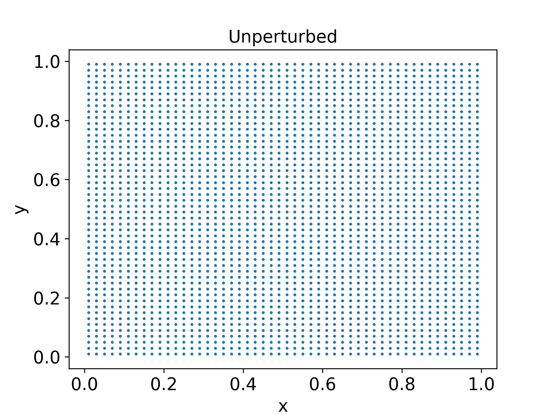
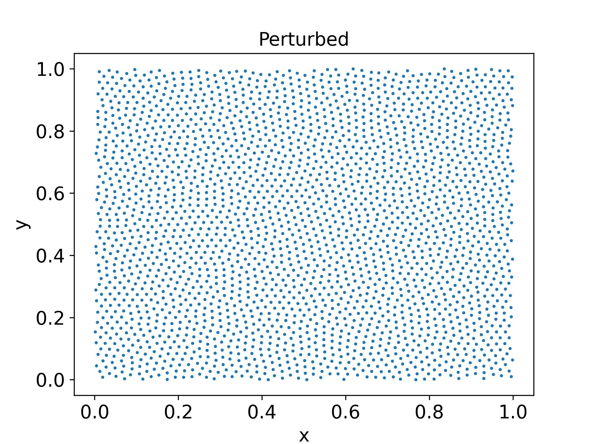
Figure 1: The unperturbed periodic particle and perturbed periodic particles.

In this section, we compare various SPH kernels for their accuracy and order of convergence in a discrete domain. We evaluate the error in function and derivative approximation in a two-dimensional periodic domain. We simulate periodicity by copying the appropriate particles and their properties near the boundary such that the boundary particles have full support Randles and Libersky (1996). The particles are either placed in a uniform mesh (unperturbed) or in a packed arrangement referred as unperturbed periodic (UP) or perturbed periodic (PP), respectively. In order to obtain the packed configuration, the particles are slightly perturbed from a uniform mesh and their positions are moved and allowed to settle into a distribution with a nearly constant density using a particle packing algorithm Negi and Ramachandran (2021). The algorithm effectively ensures that the particles are not clustered and have minimal density variations. This mimics the effect of many recent particle shifting algorithms Colagrossi et al. (2012); Lind et al. (2012a); Huang et al. (2019). In fig. 1, we show both the domains.

We compare the $L_{1}$ error in function and derivative approximation using various approximating kernels commonly used in SPH with different support radii. We present a detailed analysis in appendix A. The following is a summary of the analysis:

• Errors for function approximation on an UP domain are not affected by the choice of kernel.

• The error increases with the increase in the $h_{\Delta s}$.

• The error in a PP domain is dominated by the discretization error at higher resolutions.

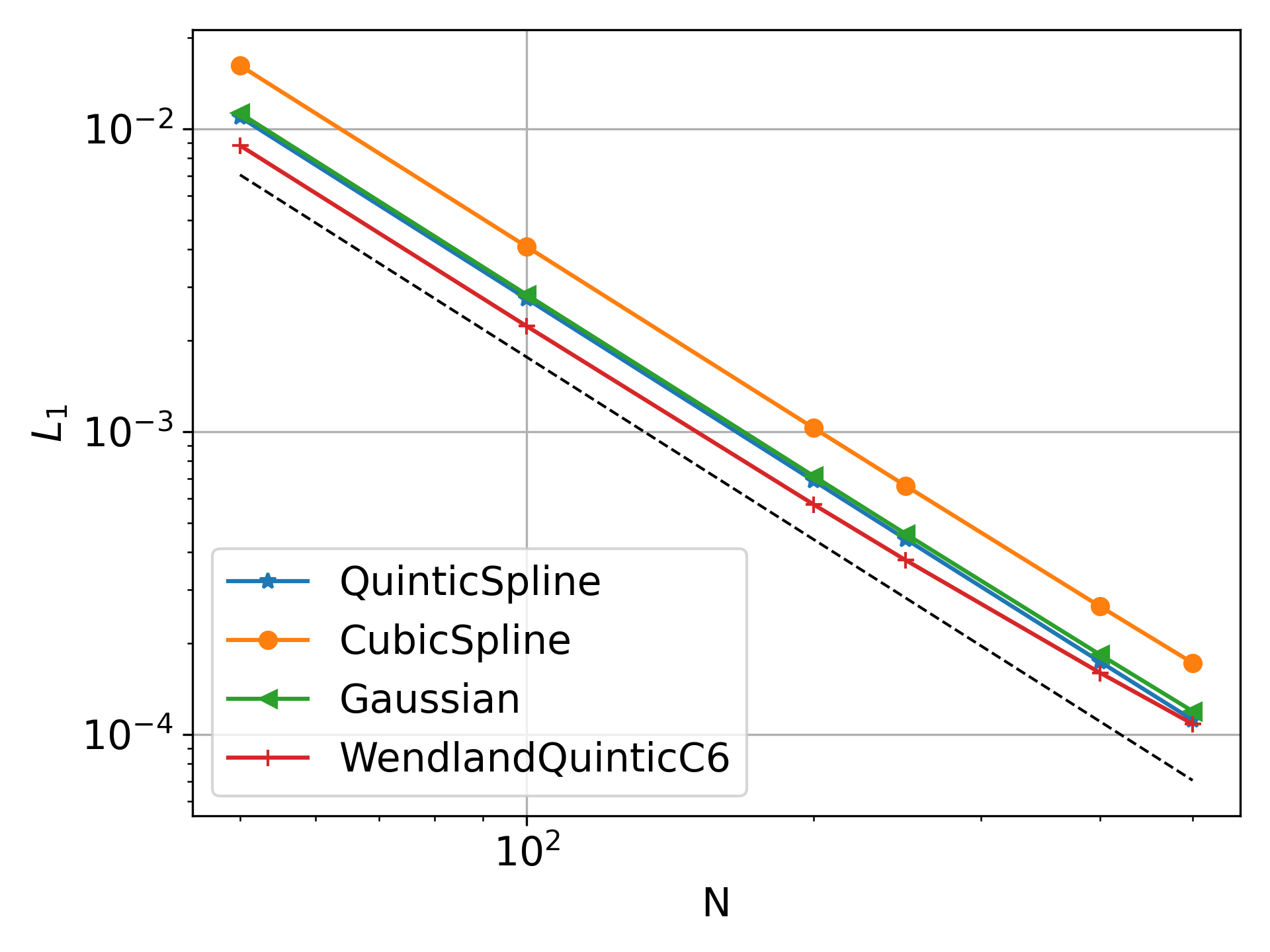
Figure 2: The convergence of the derivative approximation with different kernels when the gradient correction of Bonet and Lok (1999) is used on a PP domain. Here we use $h_{\Delta s}=1.2$.

In order to study the effect of kernel gradient correction, we apply the correction proposed by Bonet and Lok (1999) for all the selected kernels. The derivative approximation with correction is given by

$$\left<\nabla f(\mathbf{x}_{i})\right>=\sum_{j}(f(\mathbf{x}_{j})-f(\mathbf{x}_{i}))B_{i}\nabla W_{ij}\omega_{j}.$$ (7)

In fig. 2, we plot the $L_{1}$ error in the derivative approximation as a function of resolution. Clearly, all the kernels Gaussiani ($G$), Wendland quintic 6^th order ($WQ_{6}$), cubic spline ($CS$), and quintic spline ($QS$) show more or less the same behavior. Thus, we can choose any of these kernels for our convergence study of the WCSPH schemes. In the figure, it can be seen that the $WQ_{6}$ and $G$ kernels do not sustain the second-order behavior. Therefore in this work, we choose the $QS$ kernel with $h_{\Delta s}=1.2$ for all the test cases henceforth.

II.2 Considerations while applying kernel gradient correction

The SPH method is widely used to solve fluid flow problems. In this work, we focus on weakly-compressible SPH schemes that are used to simulate incompressible fluid flows. We write the Navier-Stokes equation for a weakly compressible flow along with the equation of state (EOS) as,

$$\frac{d\Varrho}{dt} =-\Varrho\nabla\cdot\mathbf{u},$$ (8a)

$$\frac{d\mathbf{u}}{dt} =-\frac{\nabla p}{\Varrho}+\nu\nabla^{2}\mathbf{u},$$ (8b)

$$p =p(\Varrho,\Varrho_{o},c_{o}),$$ (8c)

where $\Varrho$, $\mathbf{u}$, and $p$ are the fluid density, velocity, and pressure, respectively, $\nu$ is the kinematic viscosity, $\Varrho_{o}$ is the reference fluid density, and $c_{o}$ is the artificial speed of sound in the fluid. We note that the fluid density, $\Varrho$ is independent of the summation density $\rho$ (eq. 5). Normally, in SPH simulations these two are treated as the same and we discuss the reasons behind this choice in section II.4. The property, $\Varrho$ does not depend upon particle configuration and should be prescribed as an initial condition.

Name	Expression	Used in
sym1	$\frac{(p_{j}+p_{i})}{\rho_{i}\rho_{j}}\nabla W_{ij}m_{j}$	$\delta^{+}$ SPH Sun, Colagrossi, and Zhang (2018)
sym2	$m_{j}\left(\frac{p_{j}}{\rho_{j}^{2}}+\frac{p_{i}}{\rho_{i}^{2}}\right)\nabla W_{ij}$,	WCSPH Gomez-Gesteria et al. (2010),
	$\frac{V_{i}^{2}+V_{j}^{2}}{m_{i}}\tilde{p}_{ij}\nabla W_{ij}$	TVF Adami, Hu, and Adams (2013); Zhang, Hu, and Adams (2017); Ramachandran and Puri (2019), ISPH Shao and Lo (2003)
asym	$\frac{(p_{j}-p_{i})}{\Varrho_{i}}\nabla W_{ij}\omega_{j}$	WCSPH Monaghan (2005)

Table 1: Different gradient approximations for $\frac{\nabla p}{\Varrho}$. The column “expression” is assumed to be summed over the index $j$ over all the neighbor particles inside the kernel support. The term $\Varrho=\rho$ for gradient comparison. $\tilde{p}_{ij}=\frac{p_{i}\rho_{i}+p_{j}\rho_{j}}{\rho_{i}+\rho_{j}}$ is the density averaged pressure.

There are many different ways to discretize eq. 8 as can be seen from Gomez-Gesteria et al. (2010); Sun, Colagrossi, and Zhang (2018); Adami, Hu, and Adams (2013); Violeau (2012); Frontiere, Raskin, and Owen (2017); Sun et al. (2017). One of the key features of the discretization of the momentum equation (eq. 8b) is to ensure linear momentum conservation. However, some researchers trade conservation for better accuracy Sun et al. (2017) and others use a conservative form that is not as accurate Frontiere, Raskin, and Owen (2017). In view of this, we consider both conservative and non-conservative discretizations in the present study.

In table 1, we show the various pressure gradient approximations employed in different SPH schemes. The conservative forms are usually symmetric therefore are referred as sym, the non-conservative forms are asymmetric therefore referred as asym. We compare the error in the gradient approximation on both PP and UP domains with and without using a corrected kernel gradient in section B.1. We observe that only asym formulations can be corrected using all the corrections present in the SPH literature. Whereas, sym1 can be corrected by the Liu correction Liu and Liu (2006) only.

In order to explain this behavior, we take first order Taylor series approximation of a function, $f$ defined at $\mathbf{x}$ about $\mathbf{x}_{i}$ given by,

$$f(\mathbf{x})=f(\mathbf{x}_{i})+(\mathbf{x}-\mathbf{x}_{i})\cdot\nabla f(\mathbf{x}_{i})+H.O.T$$ (9)

integrating both sides with $\nabla W(\mathbf{x}-\mathbf{x}_{i})$, we get

$$\begin{split}\int f(\mathbf{x})\nabla Wd\mathbf{x}&=\int f(\mathbf{x}_{i})\nabla Wd\mathbf{x}+\int(\mathbf{x}-\mathbf{x}_{i})\cdot\nabla f(\mathbf{x}_{i})\nabla Wd\mathbf{x}\\ &=\int f(\mathbf{x}_{i})\nabla Wd\mathbf{x}+\int(\nabla W\otimes(\mathbf{x}-\mathbf{x}_{i}))\nabla f(\mathbf{x}_{i})d\mathbf{x}.\\ \end{split}$$ (10)

Using one point quadrature approximation Dilts (1999), we get

$$\begin{split}\sum_{j}f_{j}\nabla W_{ij}\omega_{j}&=\sum_{j}f_{i}\nabla W_{ij}\omega_{j}+\sum_{j}\nabla W_{ij}\otimes(\mathbf{x}_{j}-\mathbf{x}_{i})\nabla f(x_{i})\omega_{j}\\ \implies&\nabla f(x_{i})=\sum_{j}(f_{j}-f_{i})B_{i}\nabla W_{ij}\omega_{j},\\ \end{split}$$ (11)

where $B_{i}=\left(\sum_{j}\nabla W_{ij}\otimes(\mathbf{x}_{j}-\mathbf{x}_{i})\right)^{-1}$ is the correction matrix proposed by Bonet and Lok (1999). Clearly, the first order taylor-series automatically suggests correction proposed in Bonet and Lok, 1999 on an asym formulation. The eq. 11 is $O(h^{2})$ accurate Fatehi and Manzari (2011).

On the other hand, the correction proposed by Liu and Liu (2006), originates by convolving the Taylor series with $W(\mathbf{x}-\mathbf{x}_{j})$ and $\nabla W(\mathbf{x}-\mathbf{x}_{j})$, and solving all the equation simultaneously. The matrix form is given by

$$\left[\begin{array}[]{cccc}{W_{kl}V_{l}}&{x_{lk}W_{kl}V_{l}}&{y_{lk}W_{kl}V_{l}}&{z_{lk}W_{kl}V_{l}}\\ {W_{kl,x}V_{l}}&{x_{lk}W_{kl,x}V_{l}}&{y_{lk}W_{kl,x}V_{l}}&{z_{lk}W_{kl,x}V_{l}}\\ {W_{kl,y}V_{l}}&{x_{lk}W_{kl,y}V_{l}}&{y_{lk}W_{kl,y}V_{l}}&{z_{lk}W_{kl,y}V_{l}}\\ {W_{kl,z}V_{l}}&{x_{lk}W_{kl,z}V_{l}}&{y_{lk}W_{kl,z}V_{l}}&{z_{lk}W_{kl,z}V_{l}}\end{array}\right]\left[\begin{array}[]{c}{f_{k}}\\ {f_{k,x}}\\ {f_{k,y}}\\ {f_{k,z}}\end{array}\right]=\left[\begin{array}[]{c}{f_{l}W_{kl}V_{l}}\\ {f_{l}W_{kl,x}V_{l}}\\ {f_{l}W_{kl,y}V_{l}}\\ {f_{l}W_{kl,z}V_{l}}\end{array}\right],$$ (12)

where, $k$ is the destination particle index, $l$ is the neighbor particle index, $W_{kl,\beta}$ for $\beta\in{x,y,z}$ is the kernel gradient component in the $\beta$ direction. All the terms containing $l$ are summed over all the neighbor particles. On solving the eq. 12, we obtain a first order consistent gradient Liu and Liu (2006). For a constant field, this method ensures that we satisfy $\sum\tilde{W}_{ij}\omega_{j}=1$ and $\sum\nabla\tilde{W}_{ij}\omega_{j}=0$, where $\tilde{W}$ is the corrected kernel. Therefore, with this correction in both the sym1 and asym forms the second term (i.e. $*_{i}$) becomes zero, and we get the SOC approximation. Whereas, in sym2 the term $p_{i}/\rho_{i}^{2}$ does not become zero, thus even this correction fails to correct the approximation.

Using the Taylor series expansion, Fatehi and Manzari (2011) derived a correction for the Laplacian operator. In appendix C we show the error due to operators proposed by Cleary and Monaghan (1999) and Fatehi and Manzari (2011). In appendix B, we compare gradient, divergence and Laplacian approximation with corrections proposed by various authors in SPH literature. The comparison shows that the kernel gradient correction must be used appropriately for second order convergence. However, in case of divergence approximation the particle distribution plays a major role that we discuss next.

II.3 Considerations for the initial particle distribution

The particle distribution plays an important role in the error estimation of divergence approximation. In this section, we use first order Taylor series approximation to obtain error in divergence approximation as done in previous section. We consider a two-dimensional velocity field. We write the error $Er$, in the divergence evaluation as

$$Er_{i}=\nabla\cdot\mathbf{u}_{i}-\sum_{j}(\mathbf{u}_{j}-\mathbf{u}_{i})\cdot\nabla W_{ij}\omega_{j},$$ (13)

Using first order Taylor-series expansion of $\mathbf{u}_{j}$ about the point $\mathbf{x}_{i}$,

$$\mathbf{u}_{j}=\mathbf{u}_{i}-(\mathbf{x}_{ij}\cdot\nabla)\mathbf{u}_{i},$$ (14)

we write,

$$\begin{split}Er_{i}=&\left(1-\sum_{j}x_{ij}\frac{\partial W_{ij}}{\partial x}\omega_{j}\right)\frac{\partial u_{i}}{\partial x}+\left(1-\sum_{j}y_{ij}\frac{\partial W_{ij}}{\partial y}\omega_{j}\right)\frac{\partial v_{i}}{\partial y}\\ ~{}&-\sum_{j}y_{ij}\frac{\partial u_{i}}{\partial y}\frac{\partial W_{ij}}{\partial x}\omega_{j}-\sum_{j}x_{ij}\frac{\partial v_{i}}{\partial x}\frac{\partial W_{ij}}{\partial y}\omega_{j}.\end{split}$$ (15)

In the case of a UP domain, in eq. 15, the last two terms are exactly zero and the coefficient of the first two terms are of equal magnitude. Furthermore, since for a divergence-free velocity field, $\frac{\partial u_{i}}{\partial x}=-\frac{\partial v_{i}}{\partial y}$, the overall error becomes zero. On the other hand, in a PP domain, the last two terms are of equal magnitude thus cancel, and the first two terms are different to the order $10^{-4}$ (see section B.2) which becomes the leading error term. Thus, we always get an error of the order of $10^{-4}$ even after applying the Bonet correction. As far as we are aware there are no known SPH discretizations which can resolve this issue using a simple correction as done in case of gradients. This is a possible avenue for future research.

II.4 Minimal requirements for a SOC scheme

In this section, we discuss strategies to obtain a SOC scheme for weakly compressible fluid flows. We consider the fluid density as a property, $\Varrho$ carried by a particle. The numerical density, $\rho$, and volume, $\omega$ are a function of the surrounding particle distribution. The mass, $m$ of the particles satisfies $m_{i}=\Varrho_{i}V_{i}=\rho_{i}\omega_{i}$ where $V_{i}$ is the physical volume occupied by the particle and $\omega_{i}$ is the numerical volume used for integration. Thus, we can approximate the fluid density using the standard SPH approximation given by

$$\Varrho_{i}=\sum_{j}\Varrho_{j}W_{ij}\omega_{j}.$$ (16)

In case of weakly compressible SPH, the requirement of linear momentum conservation condition may be relaxed and is only satisfied approximately Oger et al. (2007); Bonet and Lok (1999); Sun et al. (2017). Therefore, we use the SOC approximations that are non-conservative as discussed in appendix B. In table 2, we list all the discretizations that we can employ to obtain a SOC WCSPH scheme.

Operators	Possible discretization for SOC
Gradient	asym_c, sym1_l
Divergence	div_c
Laplacian	coupled_c, Fatehi_c, Korzilius

Table 2: The operators and their discretization suitable for a SOC scheme (For details refer appendix B).

Furthermore, one can solve the fluid flow equations by using a Lagrangian approach as well as an Eulerian approach. We discuss the scheme for both these cases in the following sections.

II.4.1 SOC for Lagrangian WCSPH

In the Lagrangian description, the continuity equation and the momentum equation are given by

$$\begin{split}\frac{d\Varrho}{dt}&=-\Varrho\nabla\cdot\mathbf{u}\\ \frac{d\mathbf{u}}{dt}&=-\frac{\nabla p}{\Varrho}+\nu\nabla^{2}\mathbf{u},\\ \end{split}$$ (17)

In order to evaluate the RHS of the above equations, one may employ any method listed in table 2. The pressure is evaluated using an equation of state given by

$$p=\frac{\Varrho_{o}c_{o}^{2}}{\gamma}\left(\left(\frac{\Varrho}{\Varrho_{o}}\right)^{\gamma}-1\right),$$ (18)

where $\gamma=7$, $\Varrho_{o}$ is the reference density, and $c_{o}$ is the reduced speed of sound. We note that the linear equation of state where in eq. 18, $\gamma=1$, works equally well. We integrate the particles in time using a Runge-Kutta $2^{nd}$ order integrator.

Since we use an asymmetric form of the pressure gradient approximation, particles tend to clump together due to absence of a redistributing background pressure Sun, Colagrossi, and Zhang (2018). We use the iterative particle shifting proposed by Huang et al. (2019) after every few iterations to redistribute the particles. We compute the shifting vector for the $m^{th}$ iteration (of the shifting iterations) using

$$\delta\mathbf{x}_{i}^{m}=h_{i}\sum_{j}\mathbf{n}_{ij}W_{ij}\omega_{j},$$ (19)

where $\mathbf{n}_{ij}=\mathbf{x}_{ij}/|\mathbf{x}_{ij}|$. The new particle position,

$$\tilde{\mathbf{x}}_{i}^{m+1}=\mathbf{x}_{i}^{m}+\delta\mathbf{x}_{i}^{m}$$ (20)

is computed. The particles are shifted until the criterion,

$$|\max(\chi^{m})-\chi_{o}|<\epsilon$$ (21)

is satisfied up to a maximum of 10 iterations, where $\chi^{m}=h^{2}\sum_{j}W_{ij}$, $\chi_{o}$ is the value for uniform distribution, and $\epsilon$ is an adjustable parameter. In order to keep the approximation of the particle $O(h^{2})$ accurate, we update the particle properties after shifting by,

$$\phi(\tilde{\mathbf{x}}_{i})=\phi({\mathbf{x}}_{i})+(\tilde{\mathbf{x}}_{i}-\mathbf{x}_{i})\cdot\nabla\phi(\mathbf{x}_{i}),$$ (22)

where $\tilde{\mathbf{x}}_{i}$ is the final position after iterative shifting, $\phi$ is the property to be updated, and $\nabla\phi(\mathbf{x}_{i})$ is the gradient of the property on the last position computed with the Bonet correction. In a variation of the above scheme discussed in section II.6, we observe that usage of non-iterative PST proposed by Sun et al. (2019b) results in slightly higher errors but still retains its SOC. We refer to the scheme discussed above as L-IPST-C (Lagrangian with iterative PST and coupled_c viscosity formulation). Similarly the method using Fatehi_c and Korzilius formulation are referred as L-IPST-F and L-IPST-K respectively. We note that we only perform the IPST step every $10$ timesteps rather than at every timestep.

II.4.2 SOC for Eulerian WCSPH

In the Eulerian description, the continuity equation is written as

$$\frac{\partial\Varrho}{\partial t}=-\Varrho\nabla\cdot\mathbf{u}-\mathbf{u}\cdot\nabla\Varrho.$$ (23)

Since the fluid density $\Varrho$ is not same as the particle density $\rho$ we do not ignore this term, this is unlike what is done by Nasar et al. (2019). The momentum equation is written as

$$\frac{\partial\mathbf{u}}{\partial t}=-\frac{\nabla p}{\Varrho}+\nu\nabla^{2}\mathbf{u}-\mathbf{u}\cdot\nabla\mathbf{u}.$$ (24)

We discretize all the terms using SOC operators listed in table 2. We perform time integration using the RK2 integrator; however, we note that the positions of the particles are not updated.

II.5 The effect of $c_{o}$ on convergence

In the schemes discussed in the previous section, we impose artificial compressibility (AC) using the EOS, which is $O(M^{2})$ accurate Chorin (1967); Clausen (2013), where $M=U_{max}/c_{o}$ is the Mach number of the flow. Chorin (1967) originally proposed this method to obtain steady-state solutions of an incompressible flow. Some authors have used artificial compressibility with dual-time stepping to achieve truly incompressible time-accurate results Fatehi et al. (2019); Ramachandran, Muta, and Ramakrishna (2021). We achieve the incompressibility limit when $c_{o}\to\infty$. Therefore, in order to increase the accuracy at higher resolution a higher speed of sound must be used. We show the effect of the speed of sound on accuracy in section III.2.

II.6 Variations of the SOC scheme

In this section, we show that the scheme presented in the section II.4.1 (L-IPST-C) can be easily converted into other forms for improved accuracy and ease of calculation. We note that regardless of the set of governing equations employed, the discretizations from table 2 must be used to achieve SOC.

In order to remove high frequency oscillations, one could modify the continuity equation given by,

$$\frac{d\Varrho}{dt}=-\Varrho\nabla\cdot\mathbf{u}+D\nabla^{2}\Varrho$$ (25)

where, $D=\delta hc_{o}^{2}$ is the damping constant, where $\delta=0.1$. This corresponds to the $\delta$-SPH scheme Antuono et al. (2010). In this case we also use the linear equation of state to evaluate $p$ given by

$$p=c_{o}^{2}(\Varrho-\Varrho_{o}).$$ (26)

The following are different variations of the basic scheme:

1. Using different PST : One could use either IPST proposed by Huang et al. (2019) or the non-iterative PST proposed by Sun et al. (2019a). The properties like $u,v,p,$ and $\Varrho$ need to be updated using first order Taylor expansions given by

   $$\phi(\tilde{\mathbf{x}}_{i})=\phi({\mathbf{x}}_{i})+(\tilde{\mathbf{x}}_{i}-\mathbf{x}_{i})\cdot\nabla\phi(\mathbf{x}_{i})$$ (27)

   where $\phi$ is the desired property. We use the coupled formulation for the viscosity and non-iterative PST. We refer to this method as L-PST-C.

2. Using pressure evolution: On taking the derivative of EOS in eq. 26 w.r.t. time and using the eq. 25, we get the pressure evolution equation given by

   $$\frac{dp}{dt}=-\Varrho c_{o}^{2}\nabla\cdot\mathbf{u}+D\nabla^{2}p.$$ (28)

   This is very similar to the EDAC pressure evolution Ramachandran and Puri (2019). The value of $\Varrho$ can be evaluated from the EOS in eq. 26 given by

   $$\Varrho=\frac{p}{c_{o}^{2}}+\Varrho_{o}.$$ (29)

   We employ the coupled formulation for viscosity and use IPST for regularization. We refer to this method as PE-IPST-C.

3. Using remeshing for regularization: The regularization step performed using PST in the L-IPST-C method can be replaced with the remeshing procedure of Hieber and Koumoutsakos (2008). The remeshing is performed using the $M_{4}$ kernel given by,

   $$M_{4}(q)=\begin{cases}1-\frac{5q^{2}}{2}+\frac{3q^{3}}{2}&0\leq q<1,\\ \frac{(1-q)(2-q)^{2}}{2}&1\leq q<2,\\ 0&q\geq 2,\end{cases}$$ (30)

   where $q=|\mathbf{x}|/\Delta s$, where $\Delta s$ is the initial particle spacing. The properties on the regular grid are computed using

   $$\phi(\tilde{\mathbf{x}}_{i})=\frac{\sum\phi(\mathbf{x}_{j})M_{4}(|\tilde{\mathbf{x}}_{i}-\mathbf{x}_{j}|,h)}{\sum M_{4}(|\tilde{\mathbf{x}}_{i}-\mathbf{x}_{j}|,h)},$$ (31)

   where $\tilde{\mathbf{x}}$ are points on a regular Cartesian mesh. The remeshing procedure can be performed every few steps; however, we perform remeshing after every timestep. We use the coupled formulation for viscosity. We refer to this method as L-RR-C.

4. Including regularization in the form of shifting velocity: the methods of Adami, Hu, and Adams, 2013; Oger et al., 2016; Sun et al., 2019a use shifting by perturbing the velocity of the particles and adding corrections to the momentum equation. Thus the particles are advected using the transport velocity, $\tilde{\mathbf{u}}=\mathbf{u}+\delta\mathbf{u}$ and the displacement is given by,

   $$\mathbf{x}_{i}^{n+1}=\mathbf{x}_{i}^{n}+\Delta t(\mathbf{u}_{i}+\delta\mathbf{u}_{i}).$$ (32)

   The new continuity and momentum equations are given by

   $$\begin{split}\frac{\tilde{d}\Varrho}{dt}&=-\Varrho\nabla\cdot\mathbf{u}+D\nabla^{2}\Varrho+\delta\mathbf{u}\cdot\nabla\Varrho,\\ \frac{\tilde{d}\mathbf{u}}{dt}&=-\frac{\nabla p}{\Varrho}+\nu\nabla^{2}\mathbf{u}+\delta\mathbf{u}\cdot\nabla\mathbf{u},\\ \end{split}$$ (33)

   where $\frac{\tilde{d}(\cdot)}{dt}=\frac{\partial(\cdot)}{\partial t}+\tilde{\mathbf{u}}\cdot\nabla(\cdot)$. In this method, we employ SOC approximations mentioned in table 2 along with correction proposed in appendix E. We use the PST proposed in Sun et al., 2019a for this scheme along with the coupled formulation for viscosity. We refer to this method as TV-C.

5. Eulerian method: The Eulerian method solves the equation of motion on a stationary grid. This can be derived using the TV-C method by setting $\delta\mathbf{u}_{i}=-\mathbf{u}_{i}$. This substitution makes the transport velocity in the eq. 32 equal to zero, thus the particle does not move. The modified equation on setting $\delta\mathbf{u}_{i}=-\mathbf{u}_{i}$ in eq. 33, we get

   $$\begin{split}\frac{\partial\Varrho}{\partial t}&=-\Varrho\nabla\cdot\mathbf{u}+D\nabla^{2}\Varrho-\mathbf{u}\cdot\nabla\Varrho,\\ \frac{\partial\mathbf{u}}{\partial t}&=-\frac{\nabla p}{\Varrho}+\nu\nabla^{2}\mathbf{u}-\mathbf{u}\cdot\nabla\mathbf{u}.\\ \end{split}$$ (34)

   Therefore, we recover the governing equation for the Eulerian method (See section II.4.2). We note that unlike Nasar et al. (2019), we retain the last term in the continuity equation. We use the coupled formulation to discretize viscous term. We refer to this method as E-C.

III Results and discussions

In this section, we compare the solution obtained from different schemes for the Taylor-Green, Gresho-Chan vortex, and incompressible shear layer problems. We first compare the $L_{1}$ error in velocity, pressure, and linear and angular momentum conservation of the L-IPST-C with various existing schemes. In order to observe the effect of $c_{o}$ on the convergence, we solve the Taylor-Green problem with different speeds of sound using the L-IPST-C and L-IPST-F schemes. For the highest value of $c_{o}=80m/s$, we compare the results using different variations of the SOC schemes. In order to observe the conservation property, we compare the solutions for inviscid problems viz. incompressible shear layer and Gresho-Chan vortex using existing schemes as well as the SOC schemes. Furthermore, we compare the SOC scheme and existing schemes for long time simulations for all the test cases. Finally, we compute the cost of computation versus accuracy for all the schemes.

We implement the schemes using the open source PySPH Ramachandran et al. (2021) framework and automate the generation of all the figures presented in this manuscript using the automan framework Ramachandran (2018). The source code is available at https://gitlab.com/pypr/convergence_sph.

III.1 Comparison with existing SPH schemes

In this section, we compare the following schemes:

1. TVF : Transport velocity formulation proposed by Adami, Hu, and Adams (2013).

2. $\delta^{+}$SPH : The improved $\delta$-SPH formulation proposed by Sun et al. (2019a).

3. EDAC : Entropically Damped artificial compressibility SPH formulation proposed by Ramachandran and Puri (2019).

4. EWCSPH : The Eulerian SPH method proposed by Nasar et al. (2019).

5. L-IPST-C : The Lagrangian method with iterative PST and coupled_c viscosity formulation discussed in section II.4.1.

In order to compare these schemes, we consider the Taylor-Green vortex problem. We choose this problem, since it is periodic, has no solid boundaries, and admits an exact solution . The solution of the Taylor-Green problem is given by

$$\begin{split}u&=-Ue^{bt}\cos(2\pi x)\sin(2\pi y),\\ v&=Ue^{bt}\sin(2\pi x)\cos(2\pi y),\\ p&=-0.25U^{2}e^{2bt}(\cos(4\pi x)+\cos(4\pi y)),\\ \end{split}$$ (35)

where $b=-8\pi^{2}/Re$, where $Re$ is the Reynolds number of the flow. We consider $Re=100$ and $U=1m/s$. For the Lagrangian schemes, we consider a perturbed periodic (PP) arrangement of particles shown in the fig. 1 for different resolutions. At $t=0$ we initialize the pressure $p$ and velocity $(u,v)$ using eq. 35 for all the schemes. Since the fluid density $\Varrho$ is a function of pressure, we initialize density inverting eq. 18. In the case of the EWCSPH scheme, we consider an unperturbed periodic (UP) arrangement of particles and initialize the $\rho$ using the prescribed pressure. We compute the $L_{1}$ error in pressure and velocity by

$$L_{1}(f,h)=\sum_{j}\sum_{i}\frac{|f(\mathbf{x}_{i},t_{j})-f_{o}(\mathbf{x}_{i},t_{j})|}{N}\Delta t$$ (36)

where, $h=h_{\Delta s}\Delta s$ is the smoothing length of the kernel, $\Delta t$ is the timestep, $N$ is the total number of particles in the domain, $f$ is either pressure or velocity, and $f_{o}$ is the exact value obtained using eq. 35. The particle spacing, $\Delta s$ is set according to the resolution. We consider resolutions of $50\times 50$ to $500\times 500$ particles in a $1m\times 1m$ periodic domain. In order to isolate the effect of spatial approximations on the convergence, we set the timestep $\Delta t=0.3h/(U_{max}+c_{o})$, where $h=1.2/500m$ is set corresponding to highest resolution, $c_{o}=10U$, for all the simulations. We run all the simulations for $1$ timestep and observe convergence. We choose one timestep since most of the schemes considered diverge.

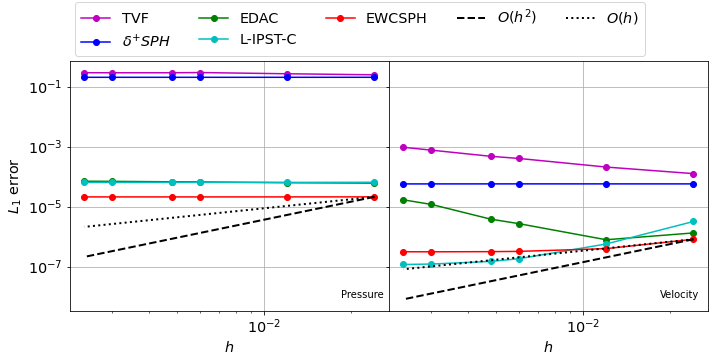
Figure 3: Convergence of $L_{1}$ error in pressure (left) and velocity (right) with the change in resolution. The $Re=100$, $c_{o}=10$, $\Delta t=6.54\times 10^{-5}$ and only $1$ timestep taken.

Name	$\frac{F_{T}}{F_{max}}$	$T_{r}$	$L_{1}(|\mathbf{u}|)(O)$	$L_{1}(p)(O)$
$\delta^{+}SPH$	2.19e-05	1.49	5.69e-05(0.00)	2.03e-01(0.00)
EDAC	1.88e-07	1.32	1.68e-05(-1.24)	7.00e-05(-0.07)
EWCSPH	7.03e-15	2.25	3.13e-07(0.38)	2.10e-05(0.00)
L-IPST-C	1.34e-05	3.36	1.18e-07(1.42)	6.41e-05(0.00)
TVF	3.70e-16	1.00	9.45e-04(-0.88)	2.88e-01(-0.07)

Table 3: Table showing total force w.r.t. the maximum force in the domain and the time taken for $1$ iteration w.r.t. the TVF scheme for all the schemes.

In the fig. 3, we plot the $L_{1}$ error evaluated using eq. 36 for pressure and velocity in the domain for different schemes. Clearly, none of the schemes show convergence in pressure. This is because the initial velocity is divergence-free, so there is no change in density and thereby pressure. We observe that the EDAC, EWCSPH, and L-IPST-C schemes are almost four orders more accurate than the TVF and $\delta^{+}$SPH schemes. In case of both the TVF and $\delta^{+}$SPH schemes, we link the pressure with particle density $\rho$, which is a function of the particle configuration. The particle positions are a result of the particle shifting, and therefore, the pressure is incorrectly captured. On the other hand, the other schemes either use a pressure evolution equation (EDAC) or a fluid density to evaluate pressure. In the case of the EWCSPH scheme, we initialize density using the pressure values in the eq. 18 which results in better accuracy.

The $L_{1}$ error in velocity diverges in the case of the TVF and EDAC schemes since these use a symmetric form of type sym2 in table 1 to discretize the momentum equation. Whereas, in the case of the $\delta^{+}$SPH scheme, sym1 type of discretization is employed leading to less errors. Moreover, the $\delta^{+}$SPH scheme uses a consistent formulation and both TVF and EDAC schemes are inconsistent when the shifting (transport) velocity is added to the momentum equation Sun et al. (2019a). The EWCSPH, and L-IPST-C formulations show convergence (not second-order) as expected. We observe that in the velocity convergence a constant leading error term dominates resulting in flattening at higher resolutions. Since, we use second-order accurate formulations in L-IPST-C and EWCSPH formulations, the only equation which is not converging with resolution is the equation of state (EOS).

In this section, we focus on highlighting the effect of using fluid density $\Varrho$ different than the numerical density $\rho$. It allows for a superior convergence rate and independence of density from particle positions. In contrast to this, the use of numerical density as a function of particle position is consistent with the volume used for the SPH approximation. In TVF, $\delta^{+}$SPH, EDAC and, EWCSPH schemes, we make no such distinction, and use the fluid density $\rho$ in the numerical volume $\omega_{j}=m_{j}/\rho_{j}$. The poor convergence for these schemes show that it is important to treat the fluid and numerical densities differently.

We also compare the linear momentum conservation and time taken to evaluate the accelerations for the case with $500\times 500$ particles. As shown in Bonet and Lok (1999), linear momentum is conserved when the total force, $\sum_{i}F_{i}=0$, where the sum is taken over all the particles and $F_{i}=\frac{\nabla p_{i}}{\Varrho_{i}}+\nu\nabla^{2}\mathbf{u}_{i}$. In the table 3, we tabulate the total force and the time taken by the scheme for one timestep with the errors and order of convergence in pressure and velocity for the $500\times 500$ resolution case. It is clear that the TVF and EWCSPH schemes conserve linear momentum and take the least amount of time. The EDAC and the $\delta^{+}$SPH scheme do not conserve linear momentum exactly. In the case of the EDAC scheme the use of average pressure in the pressure gradient evaluation results in lack of conservation. Whereas, in the case of $\delta^{+}$SPH the asymmetry of the shifting velocity divergence causes lack of conservation. The L-IPST-C scheme is known to be non-conservative; however, the value is comparable to other schemes. The time taken by the L-IPST-C scheme is significantly higher due to the evaluation of correction matrices.

III.2 Convergence with varying speed of sound

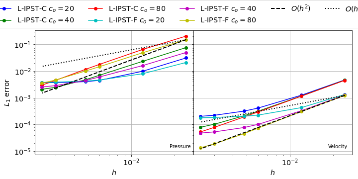
Figure 4: Convergence rates for pressure (left) and velocity (right). The L-IPST-C and L-IPST-F methods are compared for different values of $c_{o}$.

Name	$\frac{F_{T}}{F_{max}}$	$T_{r}$	$L_{1}(|\mathbf{u}|)(O)$	$L_{1}(p)(O)$
L-IPST-C $c_{o}=20$	7.13e-05	1.00	2.03e-04(1.38)	3.66e-03(0.93)
L-IPST-C $c_{o}=40$	9.31e-05	2.15	7.94e-05(1.78)	2.09e-03(1.60)
L-IPST-C $c_{o}=80$	1.44e-04	3.76	5.32e-05(1.93)	2.98e-03(1.85)
L-IPST-F $c_{o}=20$	7.11e-05	1.23	1.80e-04(0.85)	3.77e-03(0.73)
L-IPST-F $c_{o}=40$	5.99e-05	2.84	4.81e-05(1.44)	2.54e-03(1.31)
L-IPST-F $c_{o}=80$	1.66e-04	5.46	1.36e-05(1.98)	3.52e-03(1.65)

Table 4: Comparison of total force, time taken relative to the L-IPST-C with $c_{o}=20m/s$, $L_{1}$ error in velocity and order for different values of $c_{o}$.

In this section, we compare the convergence of the L-IPST-F and L-IPST-C scheme with change in AC parameter i.e. the speed of sound $c_{o}$. We consider the Taylor-Green problem; however, we run the simulation for $t=0.5s$. In fig. 4, we plot the $L_{1}$ error in the pressure and velocity for both the schemes and different $c_{o}$. We observe that both L-IPST-C and L-IPST-F methods are affected by the change in $c_{o}$ value significantly as expected. In case of pressure, with the increase in the $c_{o}$ value, the error in the lower resolutions increases; however, for higher resolution it improves. Clearly, we attain the increase in the order of convergence in case of the pressure due to increased error scales at lower resolutions. The increase in error is attributed to the inability of the SPH operators to correctly capture a divergence free velocity field as discussed in section II.3. However, on looking at the velocity convergence, both the schemes attain SOC even at higher resolutions. We observe, though, at lower resolutions, the error in the pressure increases with the $c_{o}$ value. As observed in the case of the Laplace operator comparison in B.3, the use of Fatehi_c discretization offers better accuracy.

In the table 4, we tabulate the total force, relative time, and the $L_{1}$ error in pressure and velocity with the order of convergence for $500\times 500$ particles. We observe that at a higher $c_{o}$ value, the total force is less compared to the simulation when $c_{o}$ values are lower. From the table, we can see that the use of L-IPST-F scheme offers better accuracy at the cost of the extra time taken. We also note that one can choose to use lower values of $c_{o}$ at lower resolutions and increase the value as the resolution increases to get better accuracy in pressure. Doing this does not affect the convergence in velocity.

III.3 Comparison of SOC variants

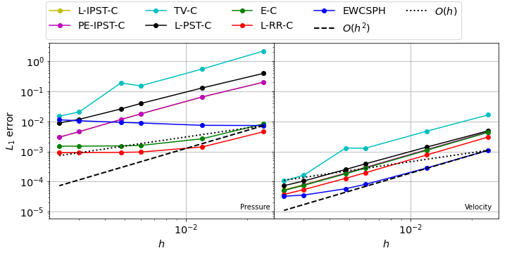
Figure 5: Convergence rates for pressure (left) and velocity (right) of different variants of SOC schemes.

Name	$\frac{F_{T}}{F_{max}}$	$T_{r}$	$L_{1}(|\mathbf{u}|)(O)$	$L_{1}(p)(O)$
E-C	8.13e-15	1.19	5.11e-05(1.94)	1.50e-03(0.71)
EWCSPH	1.07e-14	1.00	3.25e-05(1.57)	1.13e-02(-0.20)
L-IPST-C	1.44e-04	1.53	5.32e-05(1.93)	2.98e-03(1.85)
L-PST-C	2.64e-06	2.02	7.31e-05(1.84)	8.93e-03(1.68)
L-RR-C	1.51e-18	1.41	3.74e-05(1.92)	9.11e-04(0.65)
PE-IPST-C	6.17e-05	1.65	5.05e-05(1.96)	3.01e-03(1.84)
TV-C	-5.01e-06	1.88	1.06e-04(2.18)	1.51e-02(2.14)

Table 5: Comparison of total force, time taken relative to L-IPST-C with $c_{o}=20$, $L_{1}$ error in velocity and pressure for variation of schemes with $c_{o}=80$.

In this section, We simulate the Taylor-Green problem using $c_{o}=80m/s$ for a duration of $0.5s$ with different resolutions discussed in section II.6. In addition, we study the performance of the EWCSPH scheme since it is computationally efficient and accurate. In the fig. 5, we plot the error in pressure and velocity for all the schemes. In the table 5, we tabulate the total force, relative time, $L_{1}$ error in pressure and velocity at $500\times 500$ resolution, and the order of convergence.

The L-IPST-C and PE-IPST-C overlap in both the pressure and velocity convergence plots, and these are both approximately second-order. Compared to L-IPST-C, the L-PST-C shows lower convergence rate, and TV-C shows higher order of convergence, whereas E-C and L-RR-C show very poor convergence rates in pressure; however, the L-RR-C method shows very low errors in pressure. The EWCSPH has a negative convergence rate in pressure. While the TV-C shows a high convergence rate, it has much larger errors than all the other schemes considered for both pressure and velocity. The E-C, L-IPST-C, L-RR-C, and PE-IPST-C show high convergence rates in velocity as expected. The L-PST-C shows slightly high error and $1.84$ convergence rate. The EWCSPH shows a lower convergence rate of $1.57$ but is the most accurate of all the schemes regarding the velocity error.

The TV-C scheme shows low accuracy since we perform the shifting using an additional term in the momentum equation compared to the PE-IPST-C and L-IPST-C. This decrease in accuracy is also visible in the case of velocity. The L-PST-C scheme show higher error suggesting that the non-iterative PST does not perform the required amount of regularization. Both L-RR-C and E-C are comparable and most accurate. These schemes have lower error since the particles are fixed on a cartesian grid resulting in accurate computation of divergence as discussed in section II.3. The pressure convergence flattens since it reaches the limit of accuracy possible with this value of $c_{o}=80m/s$ and further accuracy may be seen by increasing this further.

Clearly, the total force in case of E-C, L-RR-C, and EWCSPH scheme is zero since we compute the acceleration on a uniform Cartesian grid of particles. However, the total force in other schemes are accurate to order $10^{-5}$. The times taken shows that L-PST-C is the highest since we apply the PST at every timestep, the TV-C involves many terms in the equations and therefore takes a lot of time. The E-C, and EWCSPH take the least time since they do not use a PST . The L-RR-C, L-IPST-C, and PE-IPST-C take a similar amount of time.

III.4 Comparison of conservation errors

Thus far, we have looked at the convergence of the various schemes. In this section, we look at the schemes listed in table 5 from the perspective of conservation of linear and angular momentum. We solve Gresho vortex and incompressible shear layer using all the schemes discussed.

III.4.1 The Grehso vortex

We consider the Gresho vortex problem Gresho and Chan (1990), which is an inviscid incompressible flow problem having the pressure and velocity fields given by,

$$p(r),u_{\phi}(r)=\begin{cases}12.5r^{2}+5,5r&0\leq r<0.2,\\ 12.5r^{2}-20r+4\ln(5r)+9,2-5r&0.2\leq r<0.4\\ 3+4\ln(2),0&0.4\leq r\\ \end{cases}$$ (37)

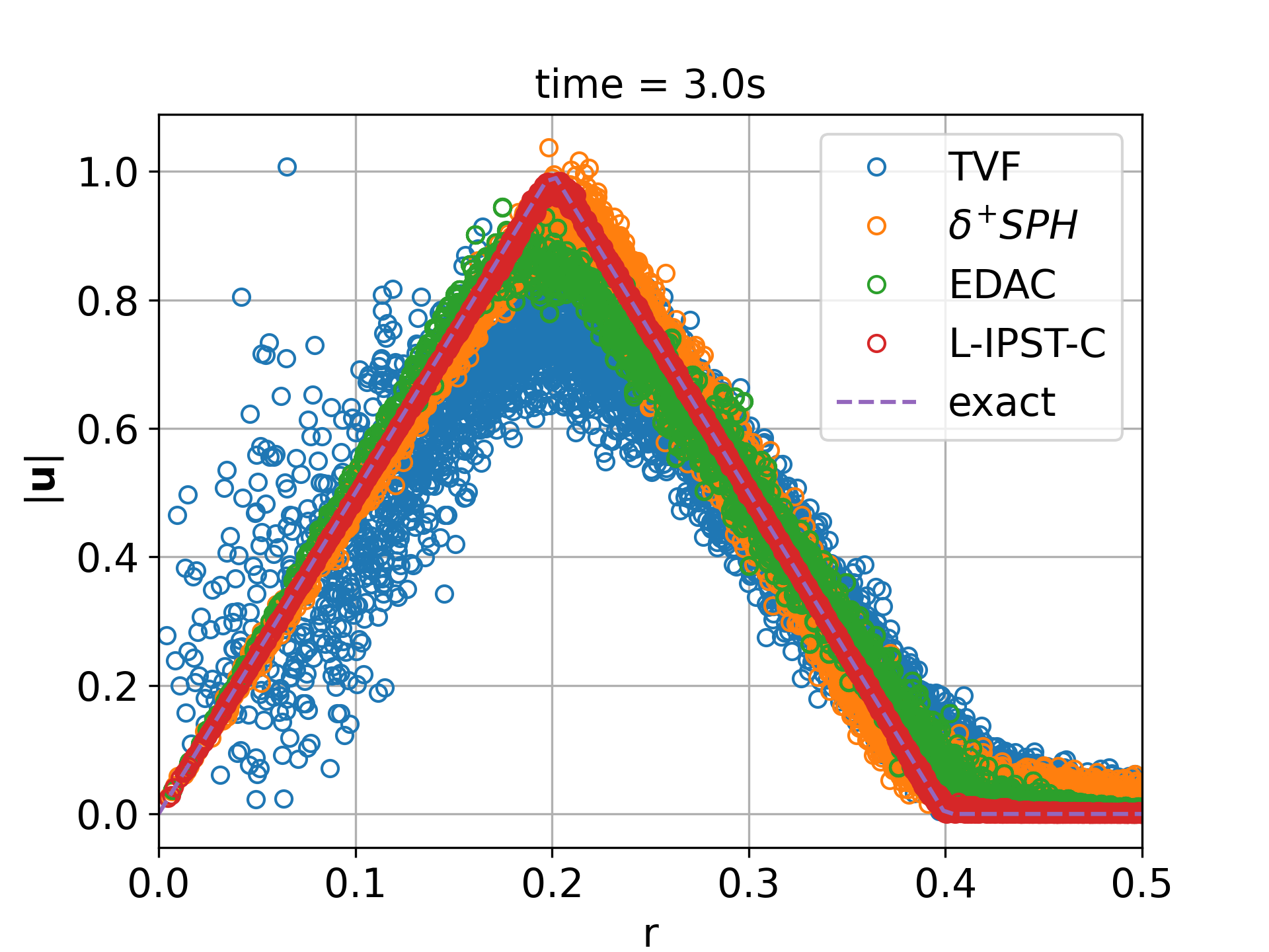
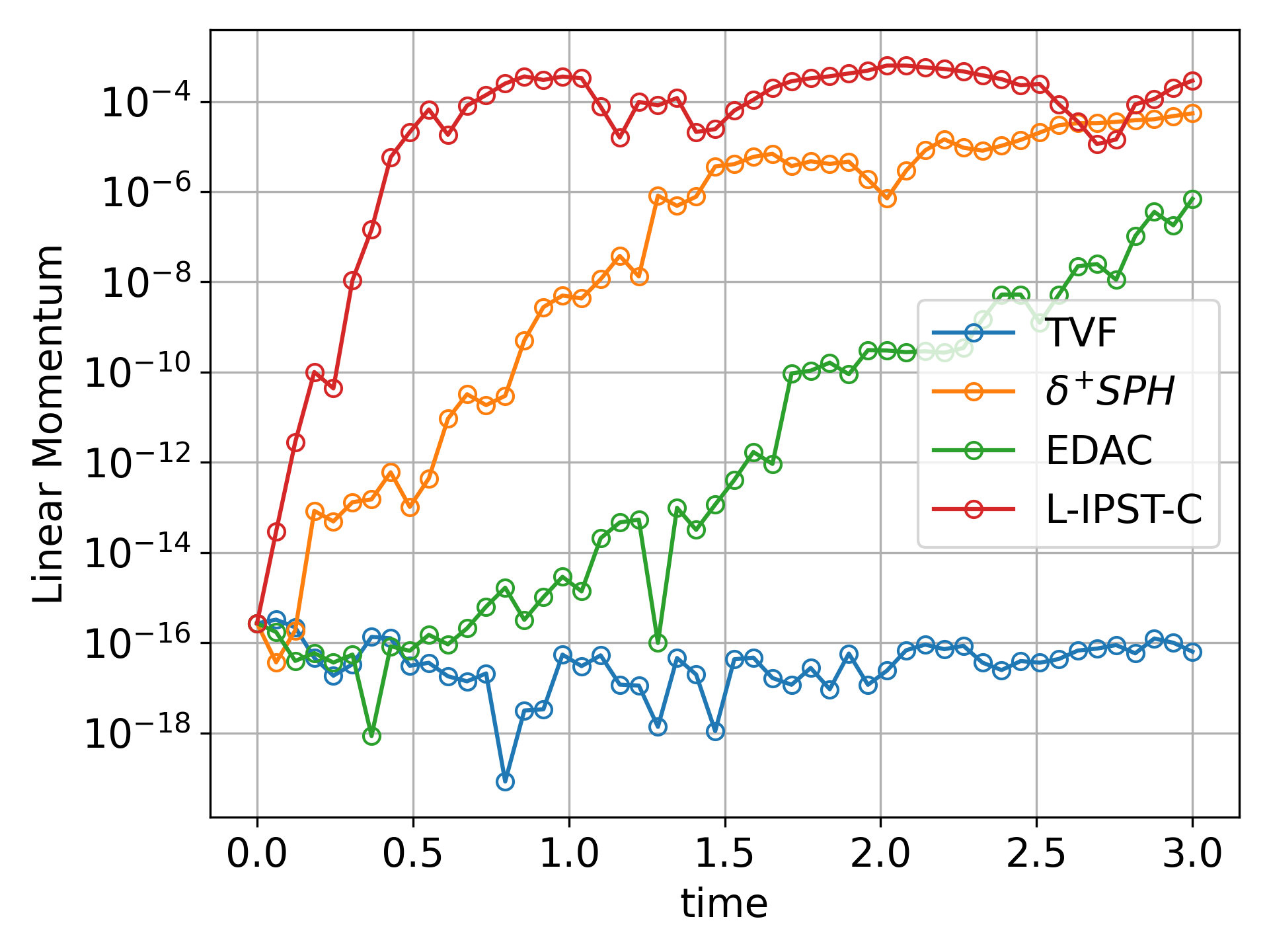
Figure 6: The velocity of particles with the distance from the center of the vortex (left) and the $x$-component of the total linear momentum (right) for all the schemes.

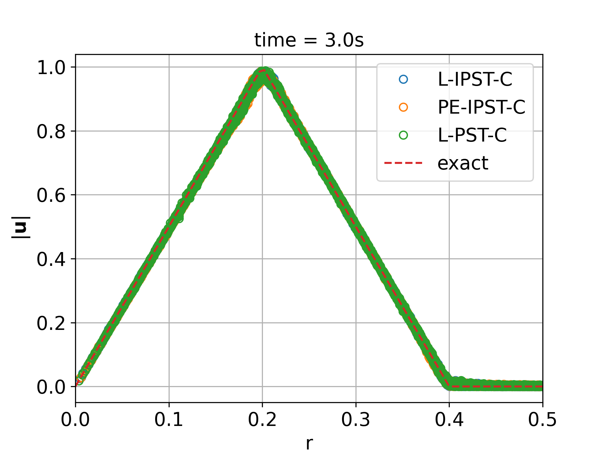
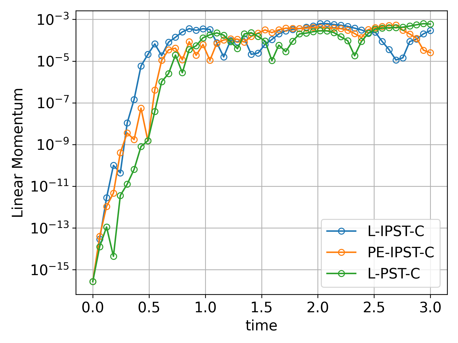
Figure 7: The velocity of particles with the distance from the center of the vortex (left) and the the $x$-component of the total linear momentum (right) for the variation of SOC scheme.

We consider an unperturbed periodic domain of size $1\times 1$ with the center at $(0,0)$. We set the kinematic viscosity, $\nu=0$, and the time step and other properties as done in the Taylor-Green problem. The problem is simulated until $t=3s$. Since the problem is inviscid, we expect the scheme to retain the velocity and pressure field. We do not use artificial viscosity in the simulations for any of the schemes. However, we use density or pressure damping as given in eq. 25 or eq. 28, respectively in order to reduce the pressure oscillations. Without this the solution becomes unstable in a short amount of time. We perform the simulation of all the schemes listed in table 3 except the EWCSPH scheme . We note that using an initial perturbed particle configuration results in very diffused results for all schemes except the L-IPST-C.

In the fig. 6, we plot the velocity of the particles with the distance, $r$ from the center (on left) and the $x$-component of the total linear momentum with time for a $100\times 100$ particle simulation. The L-IPST-C scheme retains the velocity profile very well. The $\delta^{+}$SPH, EDAC, and TVF schemes show diffusion due to inaccuracy in the pressure gradient evaluation. Except for the TVF scheme, the rest show a finite increase in the momentum bounded at $10^{-4}$. Clearly, approximate linear momentum conservation is sufficient to obtain accurate results in the case of weakly compressible flows.

We also perform the simulations with different versions of the SOC scheme listed in table 5 . In the fig. 7, we plot the velocity with the distance from the center and the $x$-component of the linear momentum with time for $100\times 100$ particle simulation. Clearly, all the schemes are accurate and approximately conserve linear momentum as expected.

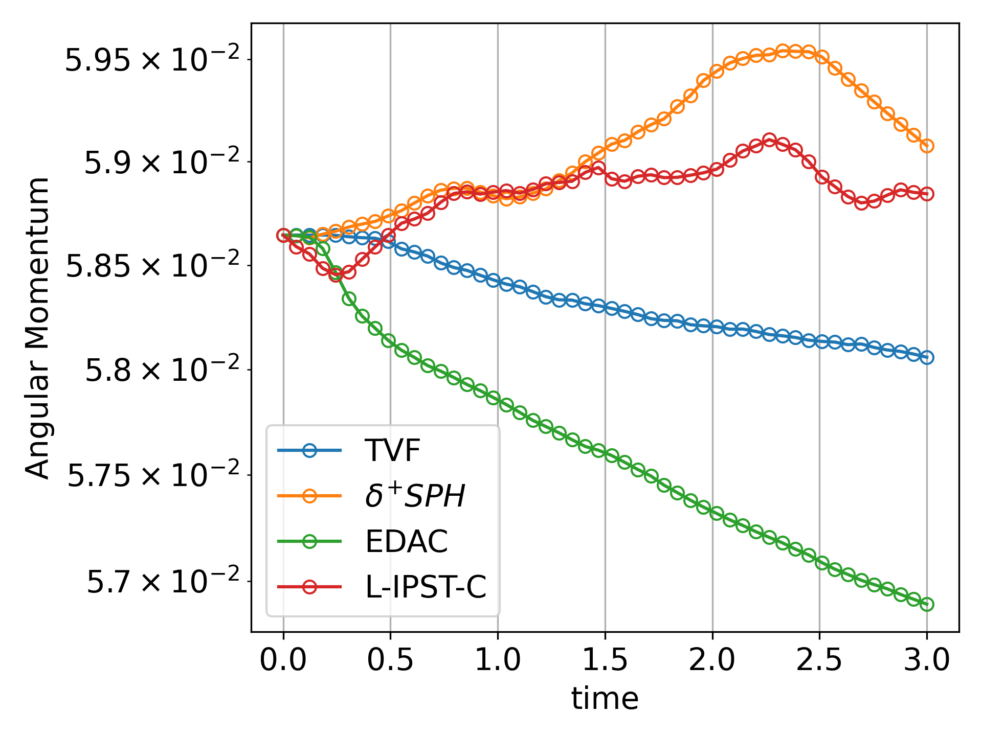
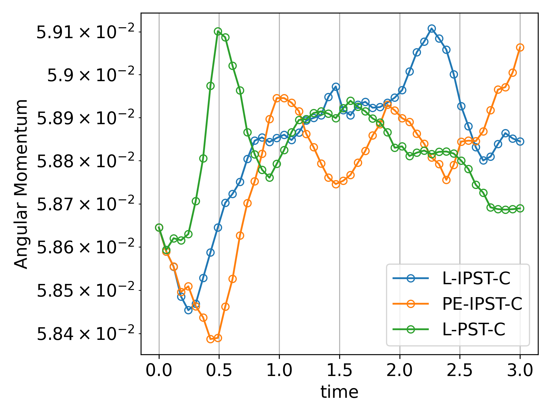
Figure 8: The angular momentum variation with time for Gresho-Chan vortex for different schemes.

In fig. 8, we show the angular momentum variation with time for different schemes. None of the schemes conserve angular momentum, but for the SOC schemes, the variations are very small and $O(5\times 10^{-4})$.

III.4.2 The incompressible shear layer

The incompressible shear layer simulates the Kelvin-Helmholtz instability in an incompressible flow. This test case produces non-physical vortices for the schemes where the operators are under resolved even when the scheme is convergent Di et al. (2005). The initial condition for the velocity in x direction is given by

$$u=\begin{cases}\tanh(\rho(y-0.25))&y\leq 0.5,\\ \tanh(\rho(0.75-y))&y>0.5,\\ \end{cases}$$ (38)

where $\rho=30$. In order to begin the instability, a small velocity is given in y direction,

$$v=\delta sin(2\pi x),$$ (39)

where $\delta=0.05$. We consider a small viscosity $\nu=1/10000$. We simulate the problem using all the schemes listed in table 3. In fig. 9 and fig. 10, we plot the vorticity field for the schemes  discussed in this paper. We note that unlike the inviscid problem of Gresho-Chan vortex, the scheme EWCSPH, TV-C and E-C shows results matching other SOC schemes. In fig. 9, we observe that TVF scheme and $\delta^{+}$SPH scheme show high frequency oscillations and while the EDAC scheme is much better; However, it shows some undesired artifacts.

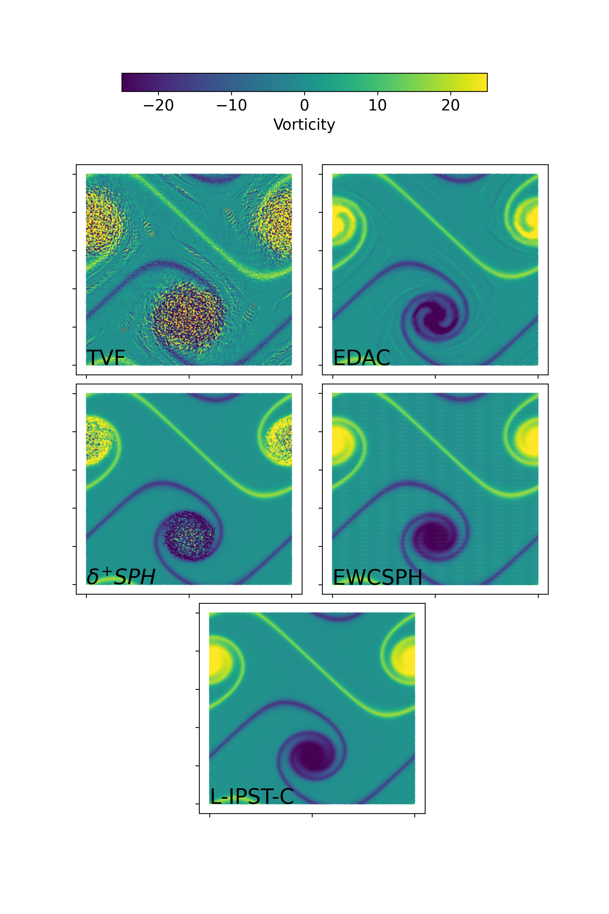
Figure 9: Vorticity contour plot for $500\times 500$ resolution for all the schemes.

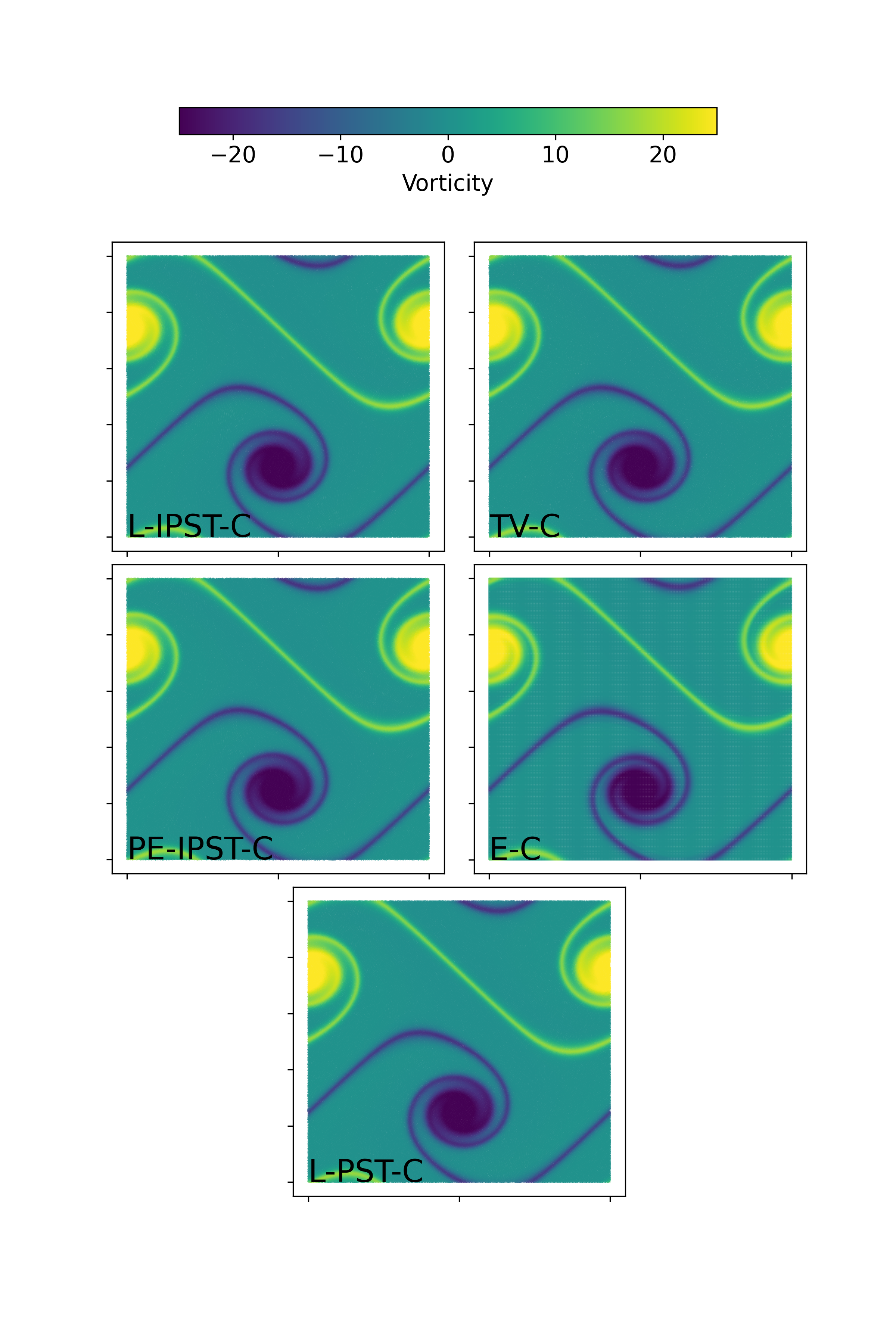
Figure 10: Vorticity contour plot for $500\times 500$ resolution for all the schemes.

III.5 Long time simulations

In this section, we study the conservation for long time simulations using the EDAC, TVF, and L-IPST-C schemes. We consider the Taylor-Green, Gresho-Chan, and Poiseuille flow problem with the same condition as before. We consider a UP particle distribution for all the schemes.

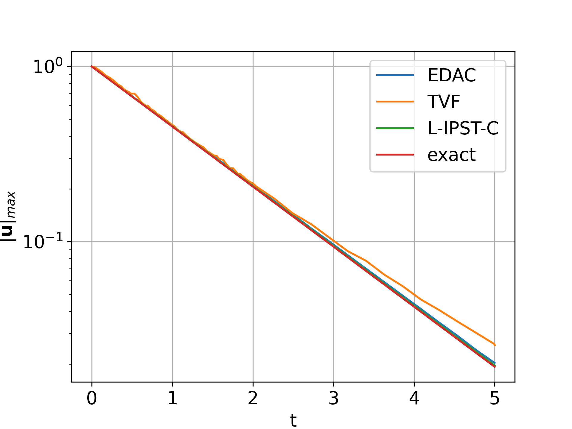
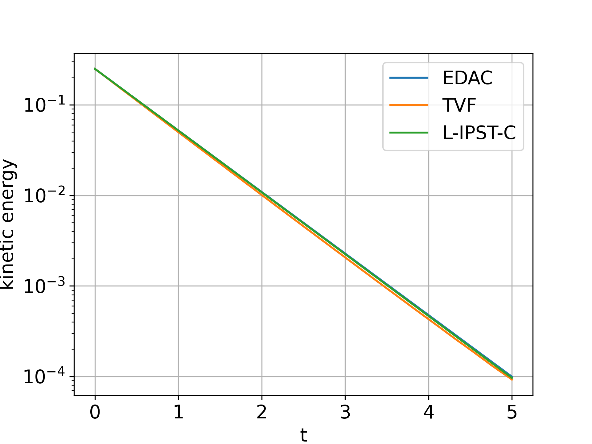
Figure 11: The maximum velocity decay and kinetic energy of the flow with respect time for Taylor-Green problem.

We simulate the Taylor-Green problem for $5s$ at $Re=100$ compared to the final time of $0.5s$ in the previous simulations for all the schemes. In fig. 11, we plot the velocity damping and the kinetic energy of the flow as a function of time. The TVF scheme shows a significant deviation from the exact result whereas the kinetic energy remains close to other scheme solutions. We note that TVF scheme conserves linear momentum exactly.

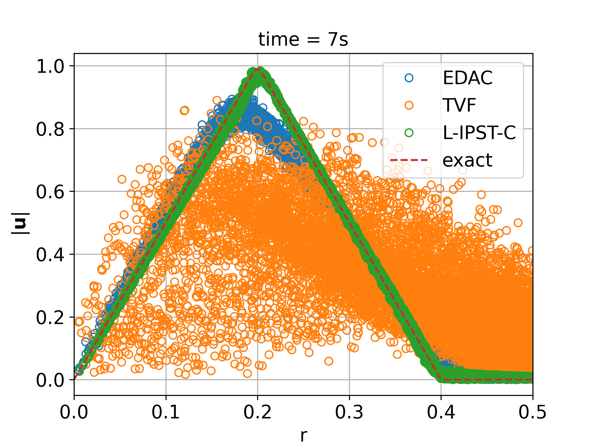
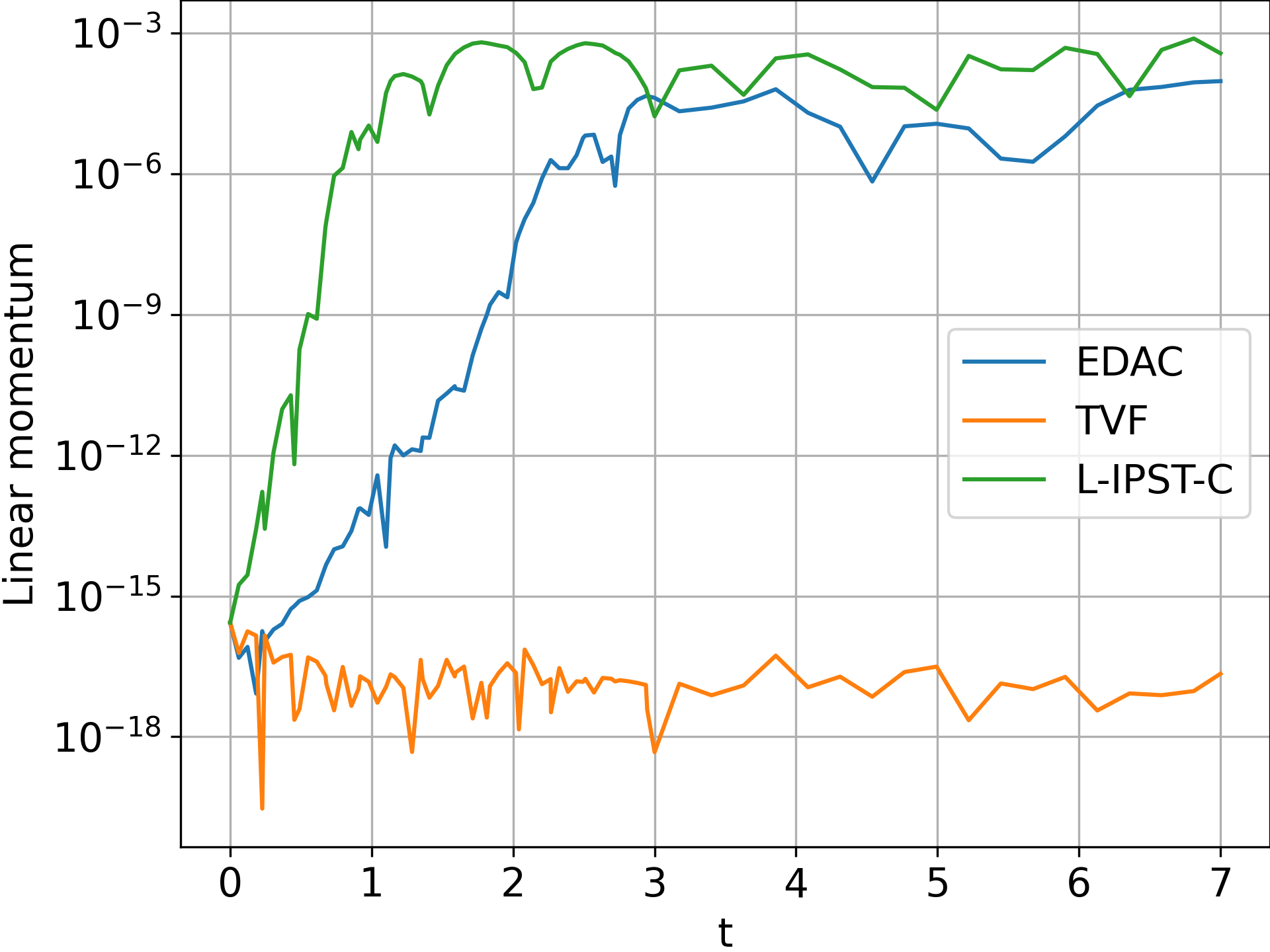
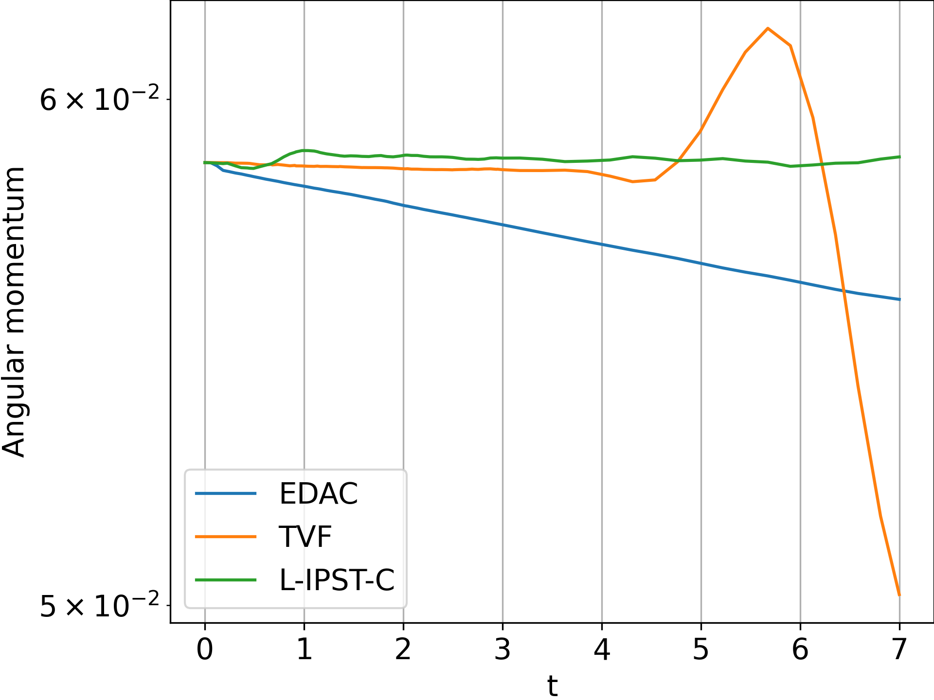
Figure 12: The velocity of particle with distance from the center, linear and angular momentum with respect to time for Gresho-Chan vortex problem.

We next simulate the Gresho-Chan vortex problem for $7s$ compared to the final time of $3s$ in section III.4.1. In fig. 12, we plot the velocity as a function of $r$, and the linear and angular momentum with respect to time for all the schemes. We observe that the TVF scheme does not capture the physics of the problem however conserves linear momentum but does not conserve angular momentum. In case of the EDAC scheme, the physics is captured better. The linear momentum is not conserved, and the solution looses angular momentum by a small amount, and the peak of the velocity distribution is not captured accurately. The L-IPST-C schemes retains the velocity field, and both the linear and angular momentum are approximately conserved. After 7 seconds the L-IPST-C schemes is no longer stable, and the velocity field is not captured accurately.

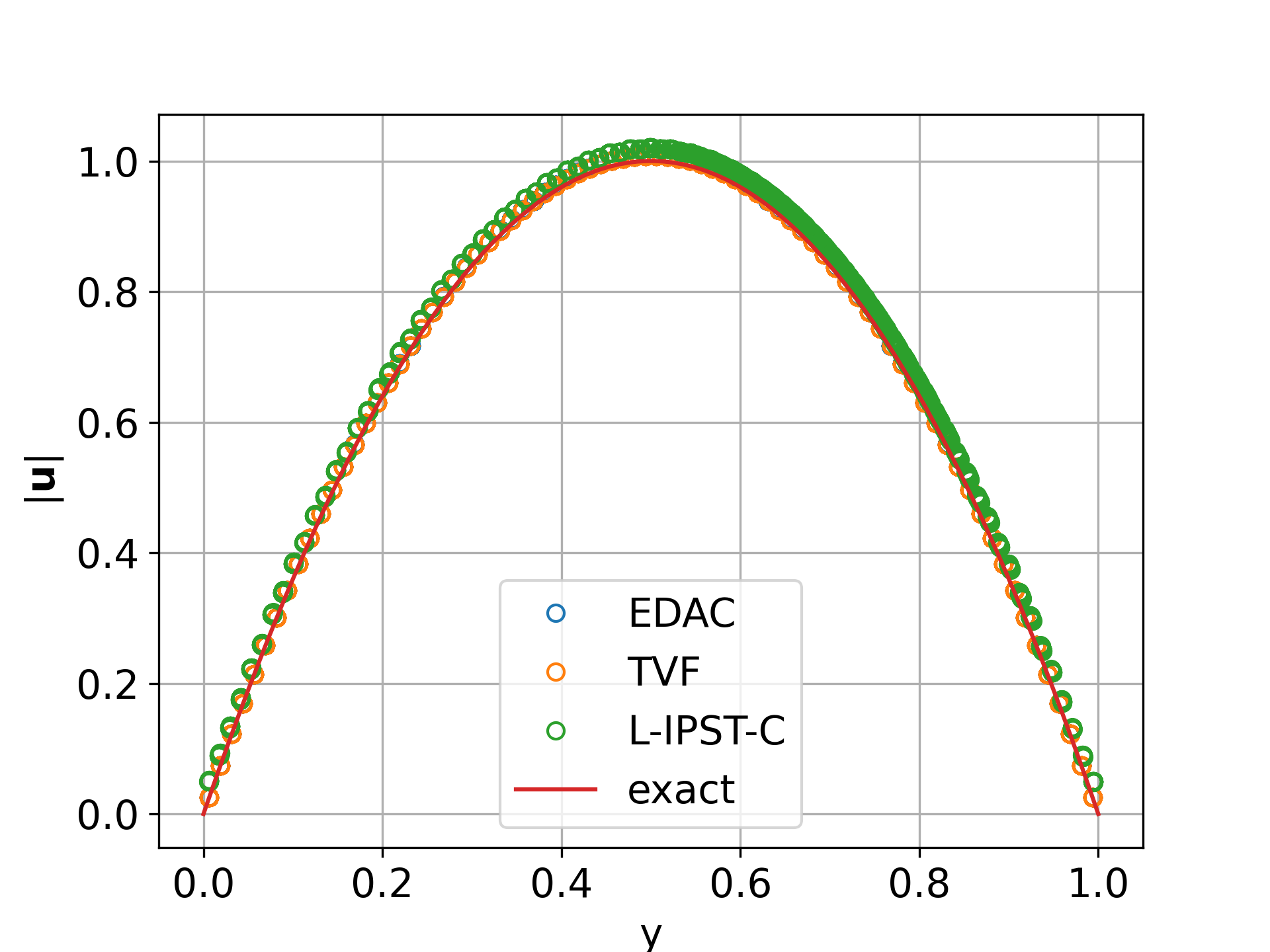
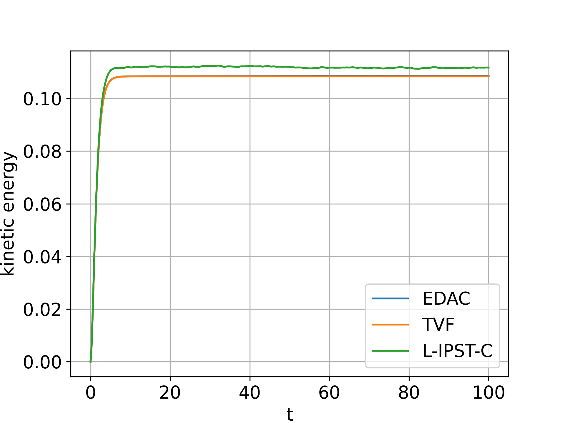
Figure 13: The $x$-component of the velocity across the plate and the kinetic energy of the flow with time for Poiseuille flow problem.

In the last test case, we simulate the Poiseuille flow problem for $100s$ compared to $10s$ in appendix D. In the fig. 13, we plot the $x$-component of the velocity and the kinetic energy of the flow with time. Cleary, all the results are similar. In case of L-IPST-C a slight deviation is observed near the wall due to approximation done near the wall (See appendix D for details).

These simulations suggests that even if a scheme is conservative like TVF it may not produce accurate results. However, for a convergent scheme like the L-IPST-C the results are accurate and despite there being no exact conservation an approximate conservation is seen.

III.6 Cost of computation

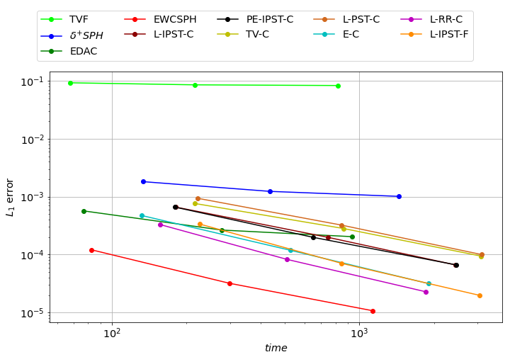
Figure 14: The $L_{1}$ error in velocity with respect to the time taken to evaluate 5000 timesteps for all the schemes discussed in the previous sections.

In this section, we compare the cost of computation of all the schemes considered in this study. We simulate the Taylor-Green problem for $5000$ timesteps with $50$, $100$, and $200$ resolutions for all the schemes. We use an Intel(R) Xeon(R) CPU E5-2650 v3 processor and execute all the simulations in serial. In fig. 14, we plot the $L_{1}$ error in velocity computed using the eq. 36 as a function of time taken for the simulation. Clearly, all the SOC schemes are close to each other in terms of errors. The E-C and EWCSPH scheme takes very less time and are very accurate; however, EWCSPH is not convergent in pressure as shown in section III.1. The EDAC scheme has lower error comparable to the SOC schemes; however, its convergence rate reduces with increase in resolution. We show that despite having higher time taken by the SOC schemes, they achieve higher accuracy with a fewer number of particle. For some schemes, these accuracy levels are not achievable at all.

IV Conclusions

In this paper, we have performed a numerical study of the accuracy and convergence of a variety of SPH schemes in the context of weakly-compressible fluids. Based on the numerical study performed in the previous sections, we summarize the key findings below.

IV.1 Choice of smoothing kernel

We first considered the SPH approximation of a function and its derivative using different kernels. All the kernels considered here show second-order convergence when the support radius is suitably chosen. The accuracy is marginally effected by the change in type of kernel. The smoothing error of an SPH approximation scales as $O(h^{2})$ and this necessitates that the smoothing length of the kernel be as small as possible. This implies that $h_{\Delta s}$ be small. As is well known, the discretization errors scale as $O((\frac{\Delta s}{h})^{\beta+2})$ and this necessitates that the smoothing radius be larger. These two requirements are contradictory. We find that by using a modest $h=1.2\Delta s$, along with the kernel corrections of Bonet and Lok (1999) or Liu and Liu (2006) we are able to obtain close to second-order convergence for the kernels considered in this work. It holds up to a resolution of $L/\Delta s=500$, where $l=1m$ which appears to be among the highest resolutions we have seen in the literature concerning the convergence of SPH methods. In the literature, we find kernels like the cubic spline to demonstrate pairing instabilities Dehnen and Aly (2012). We can avoid this instability by using a particle shifting technique (PST).

IV.2 Choice of suitable operators

The SPH approximation of operators like the gradient, divergence, and Laplacian must be chosen carefully. In this paper, we recommend two methods for gradient approximation and three methods for viscous term approximation that ensure second-order convergence. The approximations which ensure pair-wise linear momentum conservation are always divergent. In the future, one could explore pair-wise linear momentum conserving and second-order convergent SPH approximation in a perturbed domain using SPH. Furthermore, the widely used artificial compressibility assumption makes the scheme $O(M^{2})$ accurate. We recommend using high $c_{o}$ values or a dual-time stepping criteria to achieve convergence. Solving the pressure using the pressure Poisson equation may also provide SOC, although those have not been studied in this work.

IV.3 Particle density and fluid density

We recommend that one employ the fluid density in the governing differential equation as a property that convects with the particle. The approximation of the SPH operators should not be a function of a property of the fluid i.e. density. We obtain the integration volume by eq. 6 where the mass and kernel support radius of particles is kept constant. In the future, it would be important to explore the convergence of SPH operators when the mass as well as the support radius of the particles are varying as required by an adaptive SPH algorithm.

IV.4 SOC scheme and variations

We demonstrate Eulerian as well as Lagrangian SPH schemes that are second-order convergent. We show that the Eulerian schemes captures the divergence accurately due to symmetry in the particle distribution resulting in better accuracy in pressure. We derive a pressure evolution equation using the continuity equation that resembles the EDAC SPH scheme in literature. We show that the PST step in the Lagrangian method can be replaced by a remeshing step which is another moment conserving regularization. However, remeshing is not stable in the presence of jumps in the properties as observed in the case of the Gresho vortex (see appendix F) and incompressible shear layer. The PST step can be included in the momentum equation resulting in the $\delta^{+}$SPH scheme. From the $\delta^{+}$SPH method, one can obtain the Eulerian form of WCSPH method by setting the shifting velocity to $-\mathbf{u}$. All these schemes are SOC when we use a second-order convergent approximation for the operators. We show that even though the schemes are non-conservative in the absolute sense, approximate conservation also produces accurate results in the case of incompressible flows.

Thus, by a judicious choice of discretization, particle shifting, and a separation of the fluid and particle densities we have shown that second-order convergence is possible using the SPH method for weakly-compressible flows. We do observe that the SPH discretization of the divergence operator introduces errors for divergence-free fields which are noticeably absent in the case of an Eulerian method due to the symmetry of the particle distribution. This introduces significant errors into the pressure; it would be valuable to develop more accurate divergence operators for the Lagrangian case.

Given that the proposed schemes are second-order, it would be important to study the boundary conditions employed in the SPH to see how they affect the accuracy and order of convergence. A preliminary analysis performed in appendix D suggests that a popular solid-wall boundary condition Adami, Hu, and Adams (2012); Maciá et al. (2011) is not second order convergent. The accuracy of the boundary conditions will be investigated in the future.

A similar analysis in the context of variable smoothing length, and mass would be very useful in light of many recent developments of adaptive SPH methods Muta and Ramachandran (2021) One concern of note is the increased computational effort required to maintain second-order convergence and future developments in this area would be important for practical simulation using the SPH method.

Appendix A Comparison of kernels

Name	Radius	$\beta$	Remark
$G$ - Gaussian Monaghan (2005)	3	0	Truncated for low $N_{nbr}$
$QS$ - Quintic spline Ramachandran and Puri (2019)	3	3	Tensile instability
$CS$ - Cubic spline Monaghan (2005)	2	5	Paring and tensile instability
$WQ_{2}$ - Wendland $O(2)$ Wendland (1995)	2	5	No tensile or pairing instability
$WQ_{4}$ - Wendland $O(4)$ Wendland (1995)	2	8	Produces higher accuracy
$WQ_{6}$ - Wendland $O(6)$ Wendland (1995)	2	11	Produces higher accuracy

Table 6: Kernels and their properties

We consider the set of kernels listed in table 6. It covers a wide range (high order, kernels having tensile instability and pairing instability Dehnen and Aly (2012); Monaghan (2000)). In order to assess the effect of $h_{\Delta s}$ for a kernel, we perform the numerical experiment proposed by Dehnen and Aly (2012). We evaluate particle density using eq. 5 for increasing the number of neighbors $N_{nbr}$, for each of the kernels. The increase in $N_{nbr}$ corresponds to the scaling of the smoothing kernel using the $h_{\Delta s}$ parameter. In this numerical experiment, we change both the resolution and $h_{\Delta s}$.

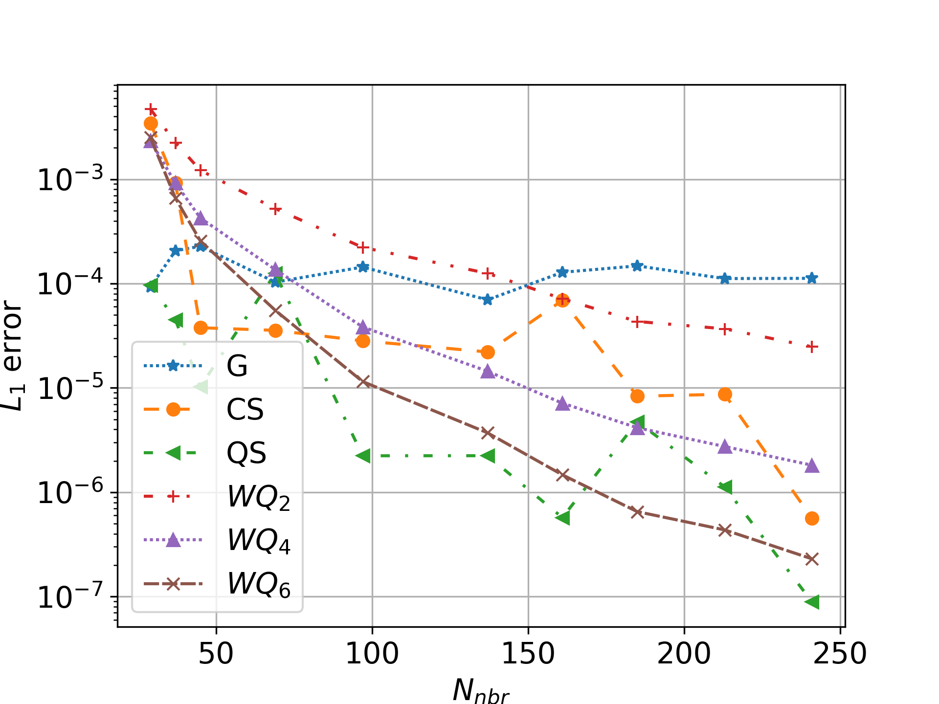
Figure 15: The particle density for different kernels with varying number of neighbors

In the fig. 15, we plot the absolute error in the particle density of one particle in an UP domain for different kernels with the change in $N_{nbr}$ under the kernel support. Clearly, the Wendland class of kernel shows a monotonic decrease in error with the increasing $N_{nbr}$. However, in the case of the $G$ and $QS$ kernels, the errors are an order less at a lower $N_{nbr}$ compared to Wendland class of kernels. The error in the $G$ kernel does not change significantly with the change in the $N_{nbr}$ compared to others. It is because we truncate the $G$ kernel to have compact support. In the $QS$, the error is lower than the $WQ_{4}$ in the entire plot. Therefore, we drop $WQ_{2}$ and $WQ_{4}$ in the subsequent investigations since it reaches the order of accuracy of $QS$ when $N_{nbr}$ is approximately $60$. High $N_{nbr}$ results in higher computational cost.

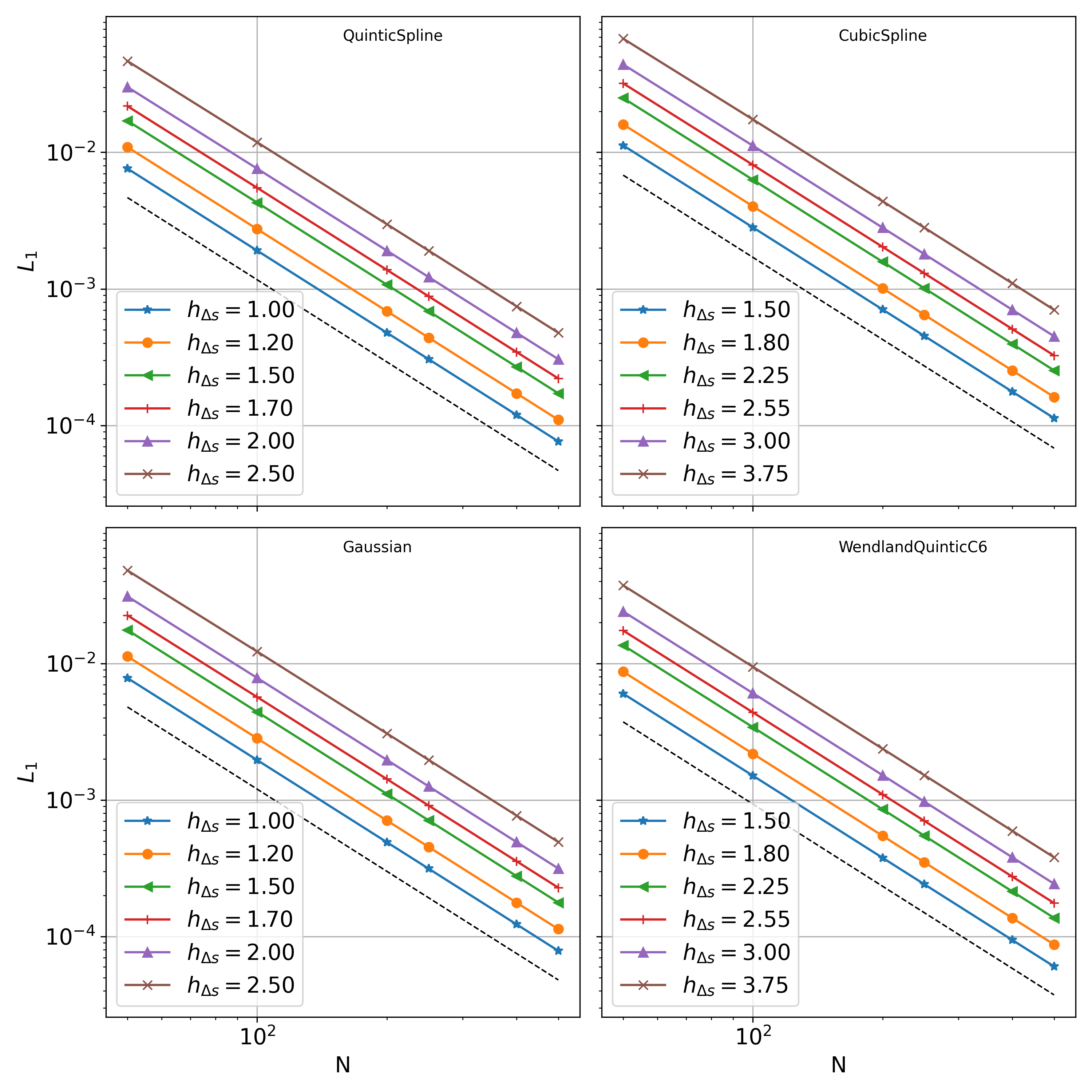
Figure 16: Order of convergence for the approximation of a function for different $h_{\Delta s}$ values in an UP domain. The dashed line shows the second order rate.

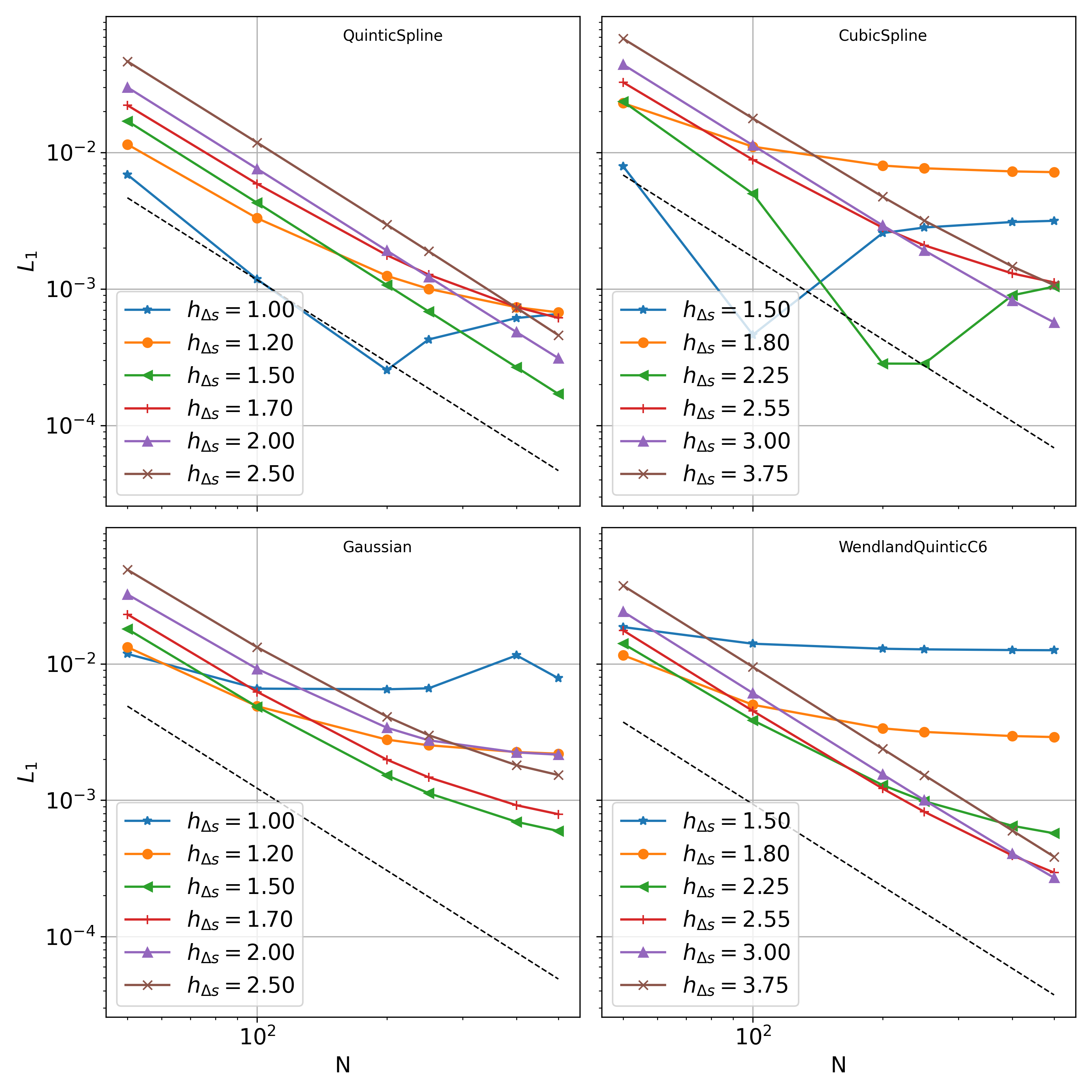
Figure 17: Order of convergence for derivative approximation for different $h_{\Delta s}$ values in an UP domain. The dashed line shows the second order rate.

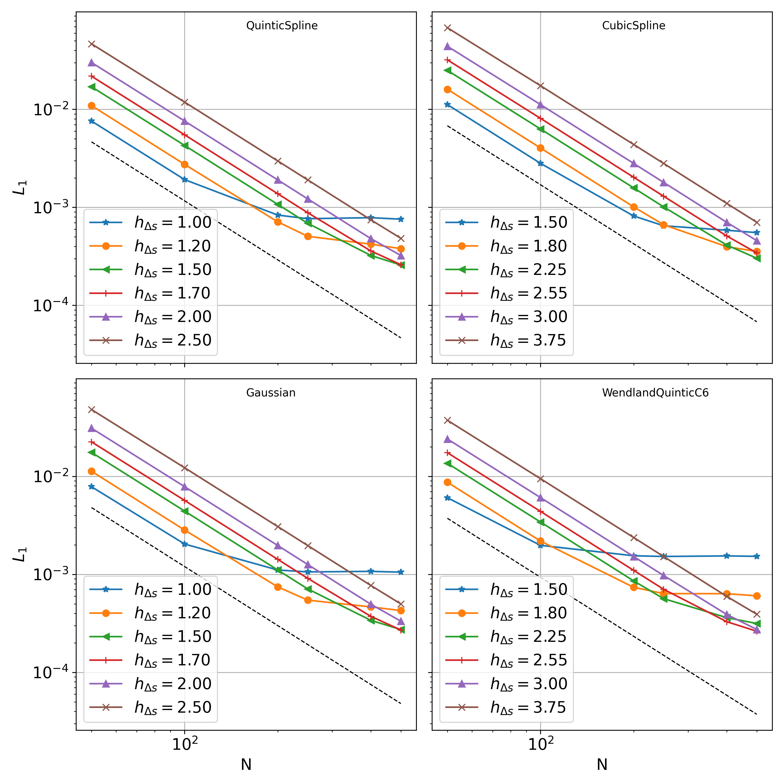
Figure 18: Order of convergence for function approximation for different $h_{\Delta s}$ values in a PP domain. The dashed line shows the second order rate.

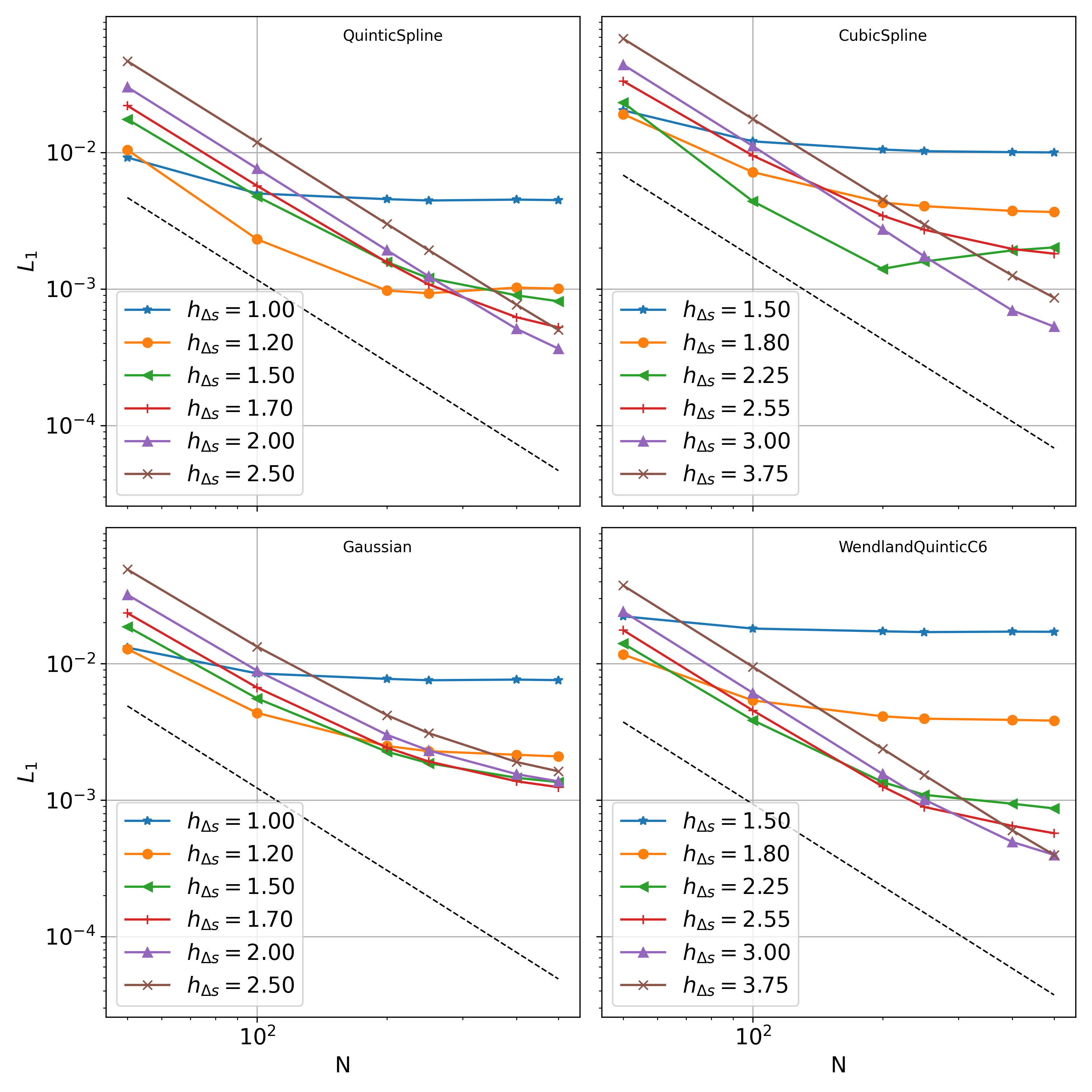
Figure 19: Order of convergence for the derivative approximation for different $h_{\Delta s}$ values in a PP domain. The dashed line shows the second order rate. The eq. 42 is used for the approximation.

We compare the four kernels $G$, $CS$, $QS$ and $WQ_{6}$ for convergence of function and its gradient approximation. We consider the field,

$$f=\sin(\pi(x+y)).$$ (40)

Given a function $g_{o}$ and its approximation $g$, we evaluate the $L_{1}$ error using,

$$L_{1}=\frac{\sum_{i}^{N}|g(\mathbf{x_{i}})-g_{o}(\mathbf{x_{i}})|}{\sum_{i}^{N}|g_{o}(\mathbf{x}_{i})|},$$ (41)

where $N$ is the total number of particles in the domain. Since the $CS$ and $WQ_{6}$ kernels have support radius of $2$ whereas, the $G$ and $QS$ kernel have support radius of $3$, we set the $h_{\Delta s}$ such that the $N_{nbr}$ is same in an UP domain. Therefore, when $h_{\Delta s}=1.0$ for $QS$ (or $G$), we take $h_{\Delta s}=1.5$ for the $CS$ (or $WQ_{6}$). For the convergence study, in this paper, we consider $50\times 50$, $100\times 100$, $200\times 200$, $250\times 250$, $400\times 400$, and $500\times 500$ resolutions for all the test cases unless stated otherwise.

A.1 Unperturbed periodic domain

In fig. 16, we plot the $L_{1}$ in the function approximation as a function of the resolution for different values of $h_{\Delta s}$ in a UP domain. We observe similar error values for all the kernels except $CS$. We obtain second-order convergence (SOC) in an UP domain upto a considerably high resolution of $500\times 500$ as expected, for all the kernels Kiara, Hendrickson, and Yue (2013a).

In fig. 17, we plot the $L_{1}$ error in the derivative approximation of the function in eq. 40 in a UP domain. The $G$ and $QS$ kernels show a better convergence rate compared to $CS$ and $WQ_{6}$ for lower $h_{\Delta s}$. The $G$ kernel does not show SOC even at $h_{\Delta s}=2.5$, since we use a truncated Gaussian. The $CS$ and $WQ_{6}$ kernel shows SOC only when $h_{\Delta s}\geq 3.0$. The $QS$ kernel shows SOC at $h_{\Delta s}>1.5$ however, a reasonable convergence can be seen for $h_{\Delta s}=1.2$ as well.

A.2 Perturbed Periodic domain

In an SPH simulation, the particles advect with different velocities, and thus the distribution of particles is no longer uniform. Some particle shifting techniques (PST) can be used to make the particle distribution uniform Xu, Stansby, and Laurence (2009); Lind et al. (2012a). Thus, it is essential to observe the convergence rate in the PP domain as well.

In fig. 18, we plot the $L_{1}$ error of the approximation of the field given in eq. 40 as a function of resolution in a PP domain for different $h_{\Delta s}$ values. The convergence rates tend to zero for higher resolution for low value of $h_{\Delta s}$ for all the kernels. The $WQ_{6}$ kernel performs worse than the $CS$ kernel at lower $h_{\Delta s}$ values however, the errors are significantly lower in $WQ_{6}$ when the $h_{\Delta s}$ value increase. On comparing $G$ and $QS$, the error plot looks exactly same except when $h_{\Delta s}=1.0$.

The SPH approximation of the gradient of a function is not even zero order accurate in a perturbed domain Nguyen et al. (2008); Kiara, Hendrickson, and Yue (2013a). The derivatives diverge when we evaluate it using eq. 3. We use a zero order consistent method proposed by Monaghan (1994) to compare the kernels. We write this approximation as,

$$\left<\nabla f(\mathbf{x}_{i})\right>=\sum_{j}(f(\mathbf{x}_{j})-f(\mathbf{x}_{i}))\nabla W_{ij}\omega_{j}.$$ (42)

In fig. 19, we plot the $L_{1}$ error in the function derivative approximation as a function of resolution using eq. 42 in a PP domain for different $h_{\Delta s}$ values and kernels. Clearly, the approximation for all the kernels shows at least zero-order convergence. The $G$ kernel does not show SOC for high $h_{\Delta s}$ which is the same as observed in the case of the UP domain. The accuracy in the case of $QS$ and $CS$ oscillates when going from lower $h_{\Delta s}$ to higher values. Zhu, Hernquist, and Li (2015) suggest that one should increase the $h_{\Delta s}$ as one increases the resolution but given the inconsistent behavior of the $CS$ and $QS$ kernels; these may not be suitable for that approach. The zero-order convergence rate occurs due to dominance of discretization error (the term $\left(\frac{\Delta s}{h}\right)^{\beta+4}$ in eq. 3) when the resolution increases in the PP domain.

Appendix B Comparison of discretization operators

B.1 Comparison of $\frac{\nabla p}{\Varrho}$ approximation

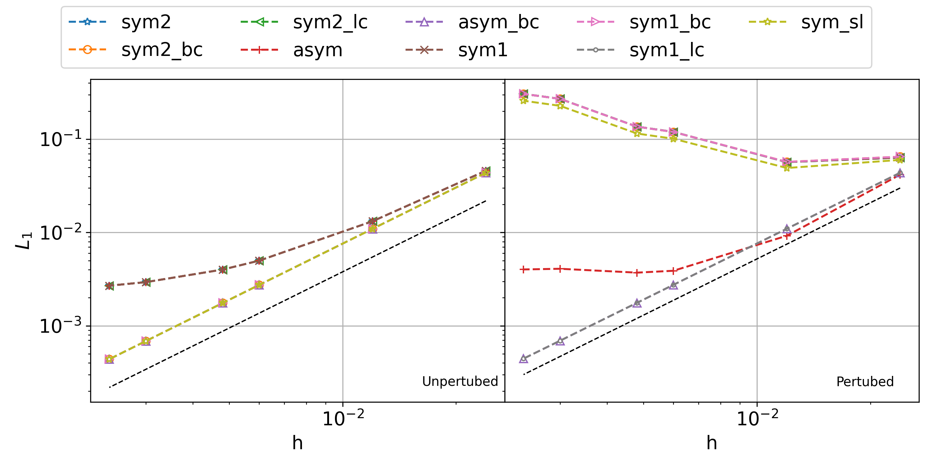
Figure 20: The rate of convergence in UP (left) and PP(right) domains for various pressure gradient listed in table 1. The dashed line shows the SOC rate. The _bc and _lc suffixes represent the corresponding form with Bonet correction Bonet and Lok (1999) and Liu correction Liu and Liu (2006). The sym_sl is the sym1 formulation with symmetrization of kernel proposed in Dilts (1999).

Name	$\frac{F_{T}}{F_{max}}$	$T_{r}$	$L_{1}(O)$
asym_bc	0.01	1.97	4.45e-04(1.98)
asym	0.00	1.00	4.02e-03(0.07)
sym1_bc	0.01	1.87	3.06e-01(-0.55)
sym1_lc	0.01	2.35	4.45e-04(1.98)
sym1	-0.00	1.05	3.06e-01(-0.55)
sym2_bc	0.01	1.87	3.06e-01(-0.55)
sym2_lc	-0.00	2.43	3.06e-01(-0.55)
sym2	-0.00	1.01	3.06e-01(-0.55)
sym_sl	-0.00	2.50	2.59e-01(-0.56)

Table 7: The ratio $\frac{F_{T}}{F_{max}}$ showing the total force in the system due to lack of conservation in the approximation, the time taken $T_{r}$ relative to the asym formulation, the $L_{1}$ error for $500\times 500$ particle in a PP domain, and last column shows the order of convergence for all the kind of formulations considered in the first column.

In this section, we compare various pressure gradient approximations. In the table 1, we list the gradient approximations considered in this study. The sym1 and sym2 are the symmetric, conservative form of the gradient approximation. We note that conservative forms have $\Varrho=\rho$. The asym is the asymmetric form. Since the SPH kernel gradient does not show SOC in a perturbed domain Quinlan, Basa, and Lastiwka (2006), we also consider the kernel correction employed to each of the approximation. In this paper, we refer to the correction proposed by Bonet and Lok (1999) as Bonet correction and the one proposed by Liu and Liu (2006) as Liu correction. We add the suffix _bc, and _lc respectively in the plots and tables to indicate these corrections. The application of corrections renders the symmetric forms non-conservative, we use the method of symmetrization of the kernel proposed by Dilts (1999) to again make it conservative. We refer to this formulation as sym_sl which we write as

$$\sum_{j}m_{j}\frac{p_{j}+p_{i}}{\rho_{j}\rho_{i}}(L_{i}\nabla W_{ij}-L_{j}\nabla W_{ji}),$$ (43)

where $L_{i}$ is the Liu correction applied to the kernel gradient . This formulation is used in the scheme proposed by Frontiere, Raskin, and Owen (2017).

In order to compare the convergence, we consider a pressure field, $p=\sin(\pi(x+y))$. We determine the $L_{1}$ error using eq. 41, where $g(\mathbf{x}_{i})$ is the pressure gradient evaluated using the approximation and $g_{o}({\mathbf{x}_{i}})$ is the exact pressure gradient. The exact pressure gradient, $\nabla p=\pi\cos(\pi(x+y))(\hat{\mathbf{i}}+\hat{\mathbf{j}})$. We compare only the x-component of the results. In fig. 20, we plot the error in the various gradient approximations discussed above in both an UP and PP domain. In the UP domain, barring the sym2_lc, all the corrected gradient approximations behave the same, whereas the uncorrected gradients do not display SOC. The corrected versions retains SOC even at high resolution since it reduces the discretization error in the approximation Fatehi and Manzari (2011); Quinlan, Basa, and Lastiwka (2006). We also observe that with the correction the second term involving the $p_{i}$ term is zero in an UP domain leading to the same expression.

In the case of the PP domain, we observe that both sym1 and sym2 and their corresponding _bc versions overlap. The symmetric formulations show an increase in the error in the approximation with increasing resolution as suggested in Fatehi and Manzari (2011). Furthermore, as discussed in section IV, the Bonet correction does not correct the symmetric formulations. Clearly, the asym formulation shows better convergence, and the Bonet correction version shows SOC. Therefore, the Bonet correction can be applied only when an asymmetric formulation is employed. Moreover, the Liu correction only corrects the symmetric form sym1, which suggests that the sym2 cannot be corrected using traditional correction techniques. Finally, the sym_sl method has a slightly lower error but looses SOC behavior due to the symmetrization of the kernel gradient. Frontiere, Raskin, and Owen (2017) reported the similar behavior.

We also compare the linear momentum conservation and time taken to evaluate the gradient for the case with $500\times 500$ particles. As shown in Bonet and Lok (1999), linear momentum is conserved when the total force, $\sum_{i}F_{i}=0$, where the sum is taken over all the particles and $F_{i}=\frac{\nabla p_{i}}{\Varrho_{i}}$. In table 7, we tabulate the ratio of total force to the maximum force ($\max(F_{i})$), the time taken to evaluate the gradient scaled by the minimum time taken by all the methods, and the $L_{1}$ error with the order of convergence , for all the formulations plotted in fig. 20. As expected, all the symmetric forms of approximation have zero total force. The asymmetric formulation has a very small total force. Clearly, the use of Bonet corrections increases the total force and slows down the computation by a factor of $2$, whereas the Liu correction makes it $2.4$ times slower. The sym_sl formulation shows zero residual force as expected. Using the table 7, we can see that asym_bc and sym1_lc show SOC and have a very low total force which makes them a suitable candidate for a scheme with SOC.

B.2 Comparison of $\nabla\cdot\mathbf{u}$ approximation

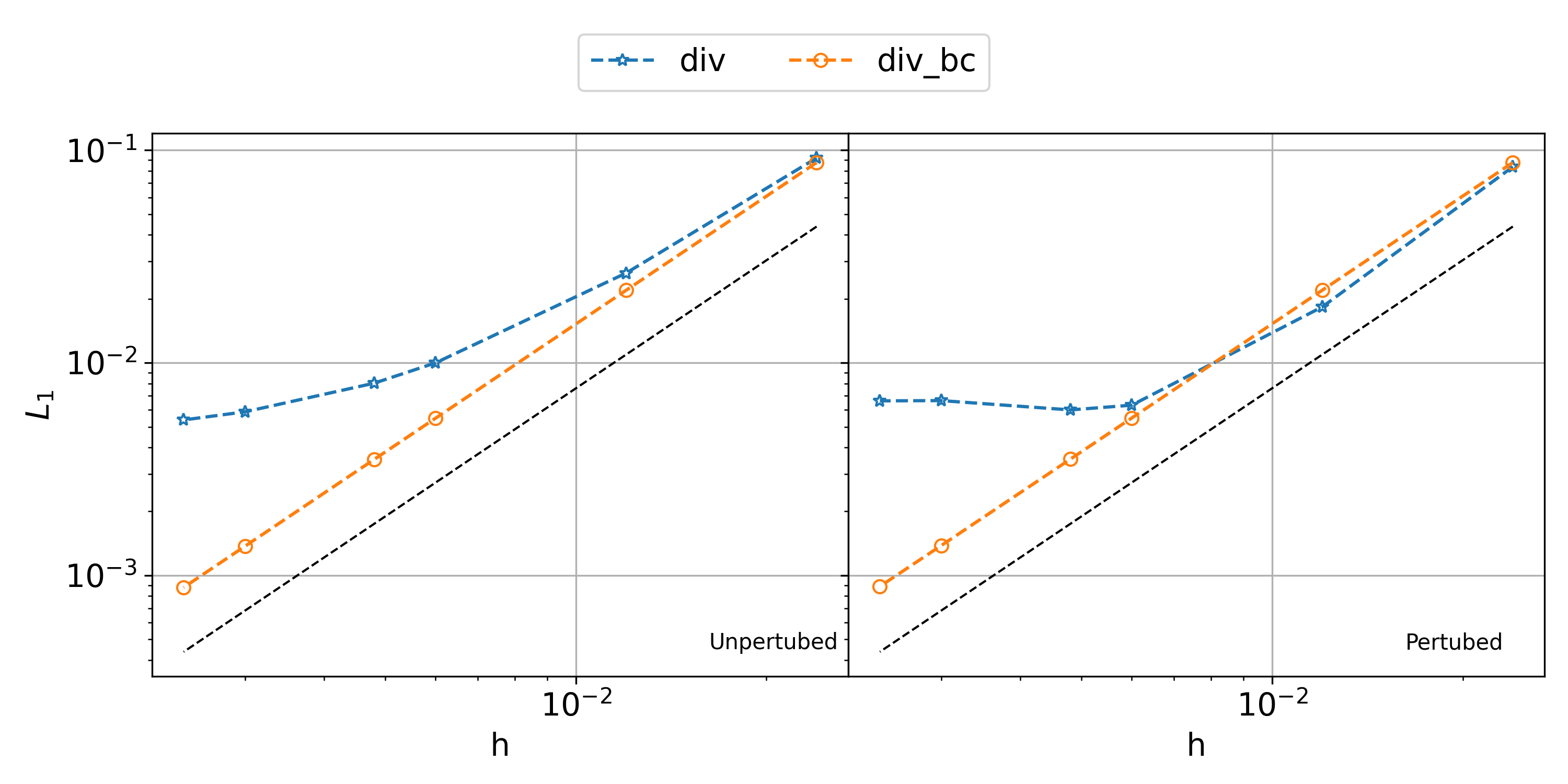
Figure 21: The rate of convergence UP (left) and PP(right) domains for velocity divergence in eq. 44. The dashed line shows the SOC rate. The suffix _bc represents the corresponding form with Bonet correction.

A zero order consistent SPH approximation for the divergence operator Monaghan (2005) is,

$$\left<\nabla\cdot\mathbf{u}\right>_{i}=\sum_{j}(\mathbf{u}_{j}-\mathbf{u}_{i})\cdot\nabla W_{ij}\omega_{j}.$$ (44)

We refer to the approximation given in eq. 44 as div. We apply the Bonet correction as done in the case of gradient approximation for a first-order consistent approximation. We refer to the corrected form as div_bc.

We consider the velocity field, $\mathbf{u}=\sin(\pi(x+y))(\hat{\mathbf{i}}+\hat{\mathbf{j}})$. The divergence of the velocity is given by, $\nabla\cdot\mathbf{u}=2\pi\cos(\pi(x+y))$. We evaluate the $L_{1}$ error in the approximation using eq. 41. In fig. 21, we plot the $L_{1}$ error in the divergence approximation in an UP and PP domain. The uncorrected approximation does not display SOC since the discretization error dominates as we approach higher resolutions. Clearly, the corrected form shows SOC even in the case of a PP domain.

In order to evaluate the accuracy of the approximation in a divergence-free field, we consider the velocity field,

$$\begin{split}u&=-\cos(2\pi x)\sin(2\pi y),\\ v&=\sin(2\pi x)\cos(2\pi y).\\ \end{split}$$ (45)

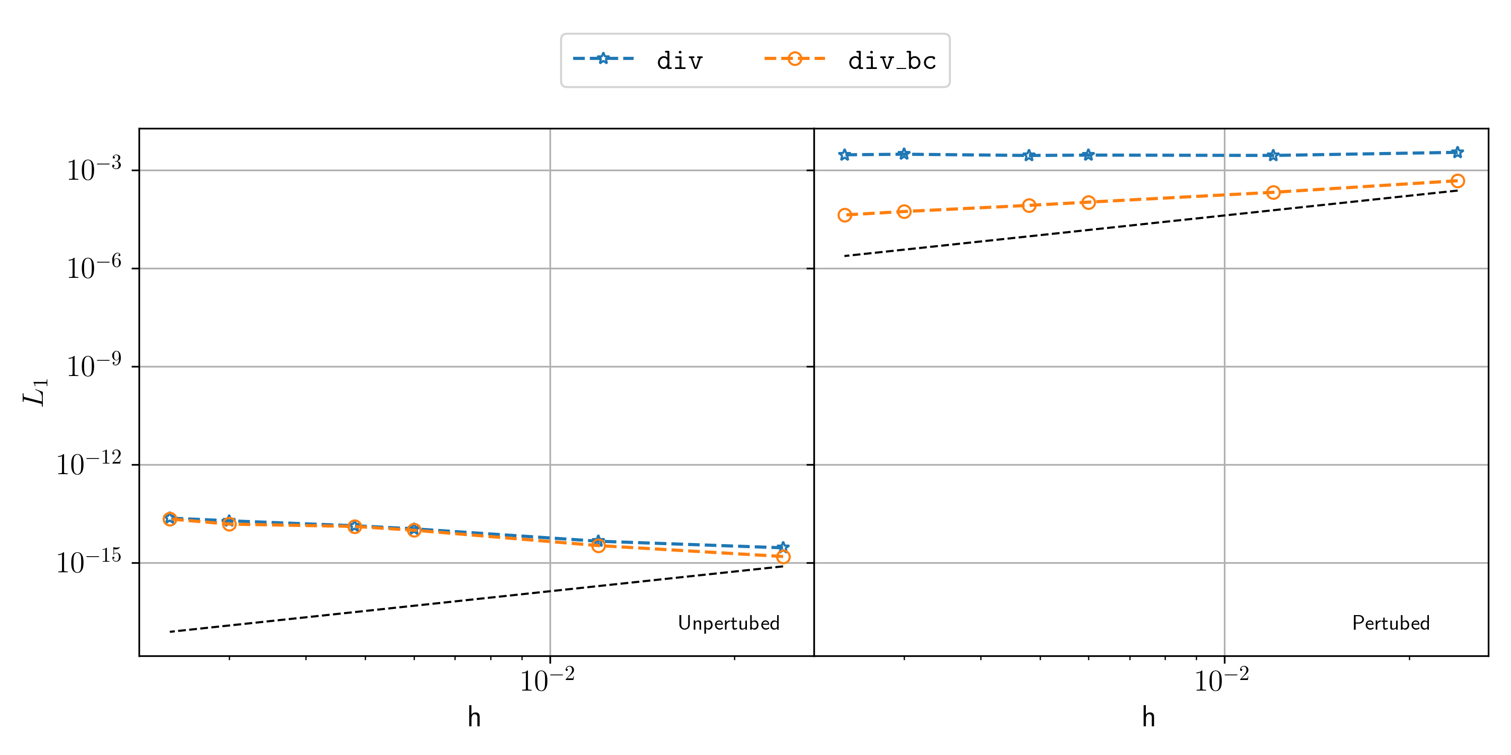
Figure 22: The rate of convergence UP (left) and PP(right) domains for velocity divergence for a divergence-free field. The dashed line shows the SOC rate. The suffix _bc represents the corresponding form with Bonet correction.

In the fig. 22, we plot the $L_{1}$ error using eq. 41 in the divergence computation as a function of resolution for the UP and PP domain. Clearly, the divergence is zero in a UP domain owing to the symmetry of the particles. However, the error in PP domain remains about the same order as seen in the case of general field in fig. 21 . Clearly, the Bonet correction does not correct this issue. We observe the implication of this behavior when we compare the schemes in section III.3.

The continuity equation corresponds to the mass conservation of the system, since mass of each particle is kept constant, we satisfy the global conservation of mass implicitly.

B.3 Comparison of $\nabla^{2}\mathbf{u}$ approximation

Name	Expression	Used in
Cleary	$2(\mathbf{u}_{i}-\mathbf{u}_{j})\frac{\nabla W_{ij}\cdot\mathbf{x}_{ij}}{|\mathbf{x}_{ij}|^{2}}\omega_{j}$	WCSPH Cleary and Monaghan (1999); Gomez-Gesteria et al. (2010)
Fatehi	$2\omega_{j}\left(\frac{(\mathbf{u}_{i}-\mathbf{u}_{j})}{|\mathbf{x}_{ij}|}-\frac{\mathbf{x}_{ij}\cdot(\nabla\mathbf{u})_{i}}{|\mathbf{x}_{ij}|}\right)\frac{\nabla W_{ij}\cdot\mathbf{x}_{ij}}{|\mathbf{x}_{ij}|}$	modified WCSPH Fatehi and Manzari (2011)
tvf	$\frac{1}{m_{i}}\left(\omega_{i}^{2}+\omega_{j}^{2}\right)(\mathbf{u}_{i}-\mathbf{u}_{j})\frac{\nabla W_{ij}\cdot\mathbf{x}_{ij}}{|\mathbf{x}_{ij}|^{2}}$	TVF Adami, Hu, and Adams (2013), EDAC Ramachandran and Puri (2019)
coupled	$((\nabla\mathbf{u})_{j}-(\nabla\mathbf{u})_{i})\cdot\nabla W_{ij}\omega_{j}$	Bonet and Lok (1999)

Table 8: The various approximations of $\nabla^{2}\mathbf{u}$. The column “expression” is assumed to be summed over the index $j$ over all the neighbor particles inside the kernel support. The $\nabla u_{i}$ term are calculated using first-order consistent formulation i.e. asym_bc

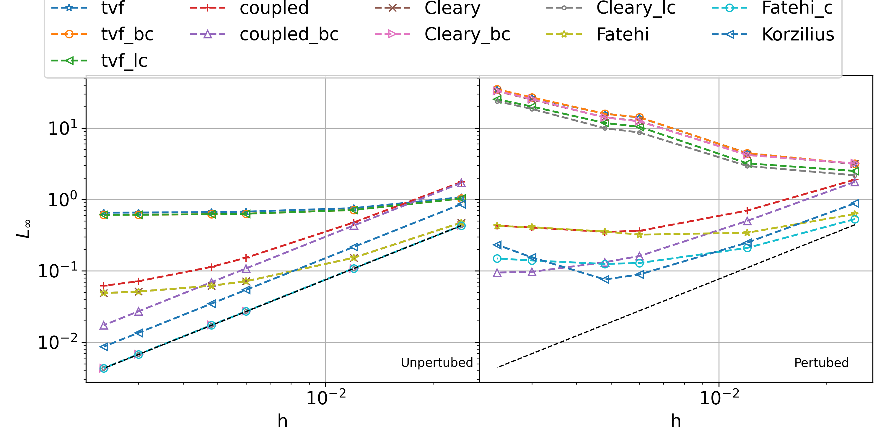
Figure 23: The rate of convergence UP (left) and PP(right) domains for various approximations of the Laplacian operator in table 8. The dashed line shows the SOC rate. The suffixes _bc and _lc represent the corresponding form with the Bonet correction and Liu correction, respectively. The Fatehi_c refers to the fatehi formulation with the correction proposed by Fatehi and Manzari (2011) (See appendix C).

Name	$\frac{F_{T}}{F_{max}}$	$T_{r}$	$L_{1}$ error	Order
Cleary_bc	-1.28e+00	1.95	6.55e-02	-0.83
Cleary_lc	-2.15e-01	2.43	4.59e-02	-0.79
Cleary	-1.08e-10	1.12	6.54e-02	-0.84
Fatehi_c	1.69e+00	4.10	2.88e-04	1.30
Fatehi	1.30e+00	2.70	8.43e-04	0.68
Korzilius	1.61e+00	4.66	2.49e-04	1.70
coupled_bc	1.61e+00	3.05	2.54e-04	1.95
coupled	1.30e+00	2.59	8.38e-04	1.46
tvf_bc	-1.26e+00	2.07	6.80e-02	-0.66
tvf_lc	-2.16e-01	2.35	5.01e-02	-0.56
tvf	-1.06e-10	1.00	6.77e-02	-0.67

Table 9: The ratio $\frac{F_{T}}{F_{max}}$ showing the total force in the system due to lack of conservation of the approximation and the time taken, $T_{r}$ relative to the tvf formulation, and $L_{1}$ error for $500\times 500$ particle case in a PP domain. The last column shows order of convergence for all the methods listed in first column.

In this section, we compare various approximations for the Laplacian operator listed in table 8. We refer to the symmetric formulations of Cleary and Monaghan, 1999; Brookshaw, 1985 as Cleary, and those of Adami, Hu, and Adams, 2013 as tvf. These ensure that linear momentum is conserved. We also consider the coupled formulation used by Bonet and Lok, 1999; Nugent and Posch, 2000 and refer to these as coupled. This formulation shows oscillations in the approximation when the initial condition is discontinuous. However, to remedy this, one can perform a first-order accurate approximation near the discontinuity and then perform this approximation as shown in Biriukov and Price, 2019. We consider the improved formulation proposed by Fatehi and Manzari (2011) referred as Fatehi. Both the coupled and Fatehi formulations are asymmetric. These formulations are performed in two steps where the first step involves computation of velocity gradient for each particle. We also consider the kernel correction applied to each of these formulations. In the case of Cleary, tvf, and coupled methods, we use the standard Bonet and Liu corrections. However, in the case of Fatehi, we use the correction tensor proposed by Fatehi and Manzari (2011) given by

$$\begin{split}\hat{B}_{i}^{\eta\mu}=&-\bigg{(}\sum_{j}\omega_{j}\partial^{\mu}W_{ij}x_{ij}^{\eta}+\\ ~{}&\sum_{j}\omega_{j}r_{ij}^{2}\partial^{\theta}W_{ij}B_{i}^{T,\theta\alpha}\sum_{j}\omega_{j}e_{ij}^{\alpha}e_{ij}^{\eta}\partial^{\mu}W_{ij}\bigg{)}^{-1},\end{split}$$ (46)

where the subscripts are SPH summation indices and superscripts are in tensor notation . We refer to this corrected formulation as Fatehi_c. Additionally, the second derivative can also be obtained by taking the double derivative of the kernel Chen and Beraun (2000); Zhang and Batra (2004); Korzilius, Schilders, and Anthonissen (2017). Therefore, we also consider the method proposed by Korzilius, Schilders, and Anthonissen (2017) that remedies the deficiencies in earlier approaches where the second derivative was employed. We obtain the second derivative of a scalar field using,

$$\tilde{\nabla^{2}}u_{i}=(\tilde{\Gamma})^{-1}\left(\sum(u_{j}-u_{i})\tilde{\nabla^{2}W}_{ij}\omega_{j}-\mathbf{x}_{ij}\left<\nabla u\right>_{i}\tilde{\nabla^{2}W}_{ij}\omega_{j}\right)$$ (47)

where $\tilde{\nabla^{2}}=\left[\frac{\partial^{2}}{\partial x^{2}},\frac{\partial^{2}}{\partial x\partial y},\frac{\partial^{2}}{\partial y^{2}}\right]^{T}$ is the operator, $\tilde{\nabla^{2}W}_{ij}=\left[\frac{\partial^{2}W_{ij}}{\partial x^{2}},\frac{\partial^{2}W_{ij}}{\partial x\partial y},\frac{\partial^{2}W_{ij}}{\partial y^{2}}\right]^{T}$. The gradient $\left<\nabla u\right>_{i}$ is approximated using the asym_bc formulation. The correction $\tilde{\Gamma}$ is given by

$$\tilde{\Gamma}_{i}=\sum\frac{1}{2}\tilde{\nabla^{2}W}_{ij}\zeta_{ij}^{T}\omega_{j}-\sum\tilde{\nabla^{2}W}_{ij}x_{ji}^{T}\omega_{j}B^{-1}\sum\frac{1}{2}\nabla W_{ij}\zeta_{ij}^{T}\omega_{j}$$ (48)

where $\zeta_{ij}=[x_{ij}^{2},x_{ij}y_{ij},y_{ij}^{2}]$ and $B$ is the Bonet correction matrix (see (11)). We refer to this formulation as Korzilius.

In the fig. 23, we plot the rate of convergence for the various formulations discussed above in both UP and PP domains. In the UP domain, all the methods at least show zeroth-order convergence. All methods without corrections suffer from high discretization error that dominates at higher resolutions Fatehi and Manzari (2011). When either Bonet or Liu corrections are employed, Cleary, coupled, Fatehi_c, and Korzilius methods show SOC. The coupled method is approximately half an order less accurate as compared to Cleary and Fatehi. The accuracy of Korzilius method is in between the coupled and Fatehi method. The tvf method is very inaccurate as the discretization error increases due to the introduction of $\omega_{i}^{2}+\omega_{j}^{2}$.

It is important to note that in the PP domain, the symmetric methods diverge due to discretization error of $O(\frac{\tilde{d}}{h^{2}}\frac{\Delta s}{h})$, where $\tilde{d}$ is the deviation from the regular particle arrangement Fatehi and Manzari (2011). Only the coupled, Korzilius, and Fatehi methods show a positive convergence rate. On applying the corresponding correction, the coupled, Korzilius, and Fatehi methods improve. The accuracy for coupled, Korzilius, Fatehi is maintained as observed in the case of UP domain.

In the table 9, we tabulate the total force as a result of the approximation, the time taken for the approximation, and the error on a PP domain consisting of $500\times 500$ particles with the order of convergence in the last column for each method plotted in fig. 23. We observe a similar increase in computational time due to the Bonet and Liu corrections as seen in the case of gradient approximation. The coupled, Korzilius, and Fatehi formulation have even higher computational cost due to the additional step of velocity gradient computation. The Korzilius method requires additional time since the double derivative of the kernel is involved. The Fatehi_c method has an additional step where we compute the second-order tensor in eq. 46 for each particle resulting in a further increase in computation time. We observe a similar increase in total force when an asymmetric version of the formulation is employed, as seen in the case of gradient approximation. Clearly, both the coupled, Korzilius, and Fatehi formulation results in an equal amount of total force resulting in a lack of conservation of linear momentum. In order to get a SOC approximation, we can use either of coupled_bc, Korzilius, or Fatehi_c formulations for viscous force estimation.

Appendix C The Cleary and Fatehi corrections

In this section, we introduce the tensor notations for SPH that makes the comprehension better. We use derivation for the error estimation from Fatehi and Manzari (2011). We write the Taylor series expansion of the velocity component, $u_{j}$ defined at a point, $\mathbf{x}_{j}$ about a point $x_{i}$ as, expansion given by

$$u_{j}=u_{i}-(\mathbf{x}_{ij}\cdot\nabla)u_{i}+\frac{1}{2}(\mathbf{x}_{ij}\cdot\nabla)^{2}u_{i}-\frac{1}{6}(\mathbf{x}_{ij}\cdot\nabla)^{3}u_{i}+\ \text{H.O.T}$$ (49)

where, $\mathbf{x}_{ij}=\mathbf{x}_{i}-\mathbf{x}_{j}$. Without loss of generality, we consider only one component of velocity. We use tensor notation to represent vector $\mathbf{x}_{ij}$ as $x_{ij}^{\alpha}$, where $i$ and $j$ are the particle indices. We follow this notation since SPH approximation is performed using sum over all its neighbors $j$. Thus, we write the eq. 49 in this tensor notation as

$$\begin{split}u_{j}=&u_{i}-x_{ij}^{\alpha}\partial^{\alpha}u_{i}+\frac{1}{2}x_{ij}^{\beta}x_{ij}^{\gamma}\partial^{\beta}\partial^{\gamma}u_{i}-\\ ~{}&\frac{1}{6}x_{ij}^{\alpha}x_{ij}^{\beta}x_{ij}^{\gamma}\partial^{\alpha}\partial^{\beta}\partial^{\gamma}u_{i}+\text{H.O.T}.\end{split}$$ (50)

We note that the subscripts are SPH notations and the superscripts are tensor notation indices.

We write the Laplacian of velocity, $\mathbf{u}$ using proposed by Cleary and Monaghan, 1999 as

$$\left<\partial^{\eta}\partial^{\eta}u\right>_{i}=\sum_{j}2\omega_{j}(u_{i}-u_{j})\frac{\partial^{\eta}W_{ij}x_{ij}^{\eta}}{r_{ij}^{2}}$$ (51)

where $\left<*\right>$ is used to denote the approximation. We write the error, $E_{i}$ in the approximation as

$$E_{i}=\partial^{\eta}\partial^{\eta}u_{i}-\left<\partial^{\eta}\partial^{\eta}u\right>_{i}$$ (52)

Using eq. 50 and eq. 51, we obtain the error,

$$\begin{split}E_{i}&=\partial^{\theta}\partial^{\theta}u_{i}-\sum_{j}2\omega_{j}\big{[}x_{ij}^{\alpha}\partial^{\alpha}u_{i}-\frac{1}{2}x_{ij}^{\beta}x_{ij}^{\gamma}\partial^{\beta}\partial^{\gamma}u_{i}+\\ &\frac{1}{6}x_{ij}^{\delta}x_{ij}^{\epsilon}x_{ij}^{\zeta}\partial^{\delta}\partial^{\epsilon}\partial^{\zeta}u_{i}+\text{H.O.T}\big{]}\frac{\partial^{\eta}W_{ij}x_{ij}^{\eta}}{r_{ij}^{2}}.\\ \end{split}$$ (53)

In the above equation, we can write $\partial^{\theta}\partial^{\theta}u_{i}=\delta^{\theta\iota}\partial^{\theta}\partial^{\iota}u_{i}$ and multiplying each term inside, we get,

$$\begin{split}E_{i}&=-\partial^{\alpha}u_{i}\sum_{j}2\omega_{j}e_{ij}^{\alpha}e_{ij}^{\eta}\partial^{\eta}W_{ij}+\\ &\bigg{(}\delta^{\beta\gamma}+\sum_{j}\omega_{j}x_{ij}^{\beta}x_{ij}^{\gamma}\frac{\partial^{\eta}W_{ij}x_{ij}^{\eta}}{r_{ij}^{2}}\bigg{)}\partial^{\beta}\partial^{\gamma}u_{i}+\text{H.O.T}\\ \end{split}$$ (54)

We can see that the first term is leading error term in the above equation. For a smoothing kernel, $W$ the term,

$$\sum_{j}\omega_{j}(\mathbf{x}_{ij}\otimes\mathbf{x}_{ij})\nabla W_{ij}$$ (55)

is the second moment of the kernel gradient. In a UP domain, the second moment is zero. However, the leading term of the error is second moment scaled by $\frac{1}{|x_{ij}|^{2}}$ which is still zero since it is a constant in a UP domain. Whereas, the leading term is non-zero and causes the approximation to deviate.

In the modified formulation proposed by Fatehi and Manzari (2011), the leading term is included in the approximation. We write the modified form as

$$\left<\partial^{\theta}\partial^{\theta}u_{i}\right>_{i}=\sum_{j}2\omega_{j}((u_{i}-u_{j})-{x}_{ij}^{\alpha}\left<\partial^{\alpha}u\right>_{i})\frac{\partial^{\eta}W_{ij}x_{ij}^{\eta}}{r_{ij}^{2}}$$ (56)

Using the similar algebraic manipulation, we write the error term as

$$\begin{split}E_{i}&=\bigg{(}\sum_{j}\omega_{j}x_{ij}^{\beta}x_{ij}^{\gamma}\partial^{\theta}W_{ij}B_{i}^{T,\theta\alpha}\sum_{j}\omega_{j}e_{ij}^{\alpha}e_{ij}^{\eta}\partial^{\eta}W_{ij}+\\ &\delta^{\beta\gamma}+\sum_{j}\omega_{j}x_{ij}^{\beta}x_{ij}^{\gamma}\frac{\partial^{\eta}W_{ij}x_{ij}^{\eta}}{r_{ij}^{2}}\bigg{)}\partial^{\beta}\partial^{\gamma}u_{i}+\text{H.O.T}\\ \end{split}$$ (57)

where $B_{i}^{T}=\left(\sum_{j}\nabla W_{ij}\otimes(\mathbf{x}_{j}-\mathbf{x}_{i})\right)^{-T}$ is the correction matrix. Fatehi and Manzari (2011) also proposed a correction for the kernel gradient. Let us assume the correction $\hat{B}_{i}^{\eta\mu}$ is applied to the kernel gradient. We write the modified equation as

$$\left<\partial^{\theta}\partial^{\theta}u_{i}\right>_{i}=\sum_{j}2\omega_{j}((u_{i}-u_{j})-{x}_{ij}^{\alpha}\left<\partial^{\alpha}u\right>_{i})\frac{\hat{B}_{i}^{\eta\mu}\partial^{\mu}W_{ij}x_{ij}^{\eta}}{r_{ij}^{2}}$$ (58)

The Error in the above equation is given by

$$\begin{split}E_{i}&=\bigg{(}\sum_{j}\omega_{j}x_{ij}^{\beta}x_{ij}^{\gamma}\partial^{\theta}W_{ij}B_{i}^{T,\theta\alpha}\sum_{j}\omega_{j}e_{ij}^{\alpha}e_{ij}^{\eta}\hat{B}_{i}^{\eta\mu}\partial^{\mu}W_{ij}+\\ &\delta^{\beta\gamma}+\sum_{j}\omega_{j}x_{ij}^{\beta}x_{ij}^{\gamma}\frac{\hat{B}_{i}^{\eta\mu}\partial^{\mu}W_{ij}x_{ij}^{\eta}}{r_{ij}^{2}}\bigg{)}\partial^{\beta}\partial^{\gamma}u_{i}+\text{H.O.T}\\ \end{split}$$ (59)

In order to make the approximation second order accurate, we must have the coefficient of $\partial^{\beta}\partial^{\gamma}u_{i}$ equal to zero. Thus we get,

$$\begin{split}\sum_{j}\omega_{j}x_{ij}^{\beta}x_{ij}^{\gamma}\partial^{\theta}W_{ij}B_{i}^{T,\theta\alpha}\sum_{j}\omega_{j}e_{ij}^{\alpha}e_{ij}^{\eta}\hat{B}_{i}^{\eta\mu}\partial^{\mu}W_{ij}+&~{}\\ \sum_{j}\omega_{j}e_{ij}^{\beta}e_{ij}^{\gamma}\hat{B}_{i}^{\eta\mu}\partial^{\mu}W_{ij}x_{ij}^{\eta}&=-\delta^{\beta\gamma}\\ \end{split}$$ (60)

On inverting the system, we obtain,

$$\begin{split}\hat{B}_{i}^{\eta\mu}=&-\bigg{(}\sum_{j}\omega_{j}\partial^{\mu}W_{ij}x_{ij}^{\eta}+\\ ~{}&\sum_{j}\omega_{j}r_{ij}^{2}\partial^{\theta}W_{ij}B_{i}^{T,\theta\alpha}\sum_{j}\omega_{j}e_{ij}^{\alpha}e_{ij}^{\eta}\partial^{\mu}W_{ij}\bigg{)}^{-1}\end{split}$$ (61)

The above equation is the correction matrix proposed by Fatehi and Manzari, 2011 in a simple tensorial notation.

Appendix D The effect of solid-wall boundary conditions

There are many solid-wall boundary condition implementations in SPH Adami, Hu, and Adams (2012); Marrone et al. (2011); Randles and Libersky (1996); Maciá et al. (2011). In this paper, we use the method due to Maciá et al. (2011) and Adami, Hu, and Adams (2012) that is widely used in SPH. In order to apply the boundary condition, a few layers of ghost particles are created outside the fluid domain such that the fluid particles near the boundary have full support. The pressure and velocity on the ghost particles are extrapolated from the fluid particles. The pressure is determined using

$$p_{g}=\frac{\sum_{f}p_{f}W_{gf}}{\sum_{f}W_{gf}},$$ (62)

where $p_{f}$ is the pressure of the fluid particles, $W_{gf}$ is the kernel weight between the ghost and fluid particle, and the sum is taken over all the fluid particles near the ghost particle. The velocity on the ghost particle is extrapolated using

$$u_{g}=2u_{s}-\frac{\sum_{f}u_{f}W_{gf}}{\sum_{f}W_{gf}},$$ (63)

where $u_{s}$ is the actual velocity of the solid, and $u_{f}$ is the velocity of the fluid particles. In the L-IPST-C scheme, we use a slip boundary for the continuity equation Muta, Ramachandran, and Negi (2020). Additionally, since the coupled formulation is prone to oscillations due to discontinuity Quinlan, Basa, and Lastiwka (2006) we smooth-out oscillations from the three fluid particle layers adjacent to the wall by setting velocity values using a first order consistent interpolation.

We consider the Poiseuille flow problem. The exact solution of the Poiseuille flow is given by

$$u(y)=0.5\frac{F}{\nu}y(L-y)$$ (64)

where $F=0.8N$ is the constant force applied on the flow, $\nu=0.1m^{2}/s$ is the dynamic viscosity of the flow, $L=1m$ is the distance between the parallel plates, and $y$ is the distance from the bottom plate. We consider a domain of size $0.4\times 1m^{2}$ with maximum flow velocity $U=1m/s$ and $Re=10$. The domain is periodic in $x$-direction. We simulate the problem for $10s$ for each scheme for $50\times 50$, $100\times 100$, and $200\times 200$ resolutions.

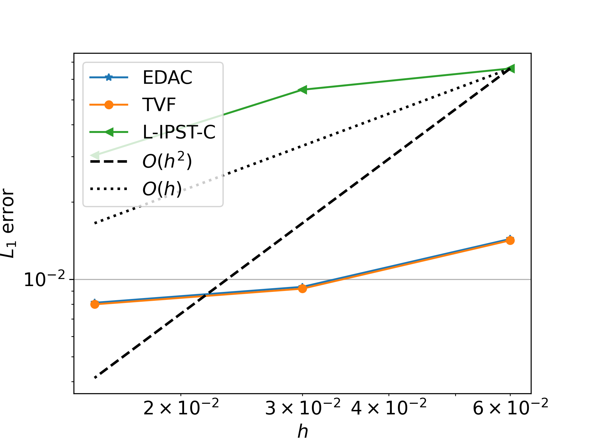
Figure 24: The convergence of error in the $x$-component of the velocity for Poiseuille flow problem.

In fig. 24, we plot the $L_{1}$ error in the $x$-component of the velocity for all the schemes. Clearly, none of the schemes show convergence. The L-IPST-C scheme shows a higher value of error due to the smoothing used for the near wall fluid particles. It is clear from the above experiment that we require a convergent boundary condition implementation such that it does not dominate the error in the solution.

Appendix E $\delta^{+}$SPH formulation correction

The the evolution equation of the $\delta^{+}$SPH equation has the form

$$\frac{Df}{Dt}=\frac{df}{dt}+\nabla f\cdot\delta\mathbf{u},$$ (65)

where $\frac{Df}{Dt}=\frac{\partial f}{\partial t}+(\mathbf{u}+\delta\mathbf{u})\cdot\nabla f$. The above equation can be written in terms of a particle $i$ as,

$$\frac{Df_{i}}{Dt}=\frac{df_{i}}{dt}+\nabla f_{i}\cdot\delta\mathbf{u}_{i}.$$ (66)

We can use the vector identity for the last term,

$$\begin{split}\nabla f\cdot\delta\mathbf{u}=\nabla\cdot(f\delta\mathbf{u})-f\nabla\cdot(\delta\mathbf{u}).\end{split}$$ (67)

On performing SPH approximation, we obtain

$$\begin{split}\nabla f_{i}\cdot\delta\mathbf{u}_{i}&=\sum_{j}(f_{j}\delta\mathbf{u}_{j}-f_{i}\delta\mathbf{u}_{i})\cdot\nabla W_{ij}\omega_{j}-\\ ~{}&\sum_{j}f_{i}(\delta\mathbf{u_{j}}-\delta\mathbf{u}_{i})\cdot\nabla W_{ij}\omega_{j}\\ &=\sum_{j}(f_{j}-f_{i})\delta\mathbf{u}_{j}\cdot\nabla W_{ij}\omega_{j}.\end{split}$$ (68)

Clearly, we cannot recover the LHS should we use the above discretization. However, on using $f_{j}$ in place of $f_{i}$ in the second term, we get

$$\begin{split}\nabla f_{i}\cdot\delta\mathbf{u}_{i}&=\sum_{j}(f_{j}\delta\mathbf{u}_{j}-f_{i}\delta\mathbf{u}_{i})\cdot\nabla W_{ij}\omega_{j}-\\ ~{}&\sum_{j}f_{j}(\delta\mathbf{u_{j}}-\delta\mathbf{u}_{i})\cdot\nabla W_{ij}\omega_{j}.\\ &=\sum_{j}(f_{j}-f_{i})\delta\mathbf{u}_{i}\cdot\nabla W_{ij}\omega_{j}.\end{split}$$ (69)

Thus, in the $\delta^{+}$SPH we should use the above discretization.

Appendix F Schemes with issues solving the Gresho-Chan vortex

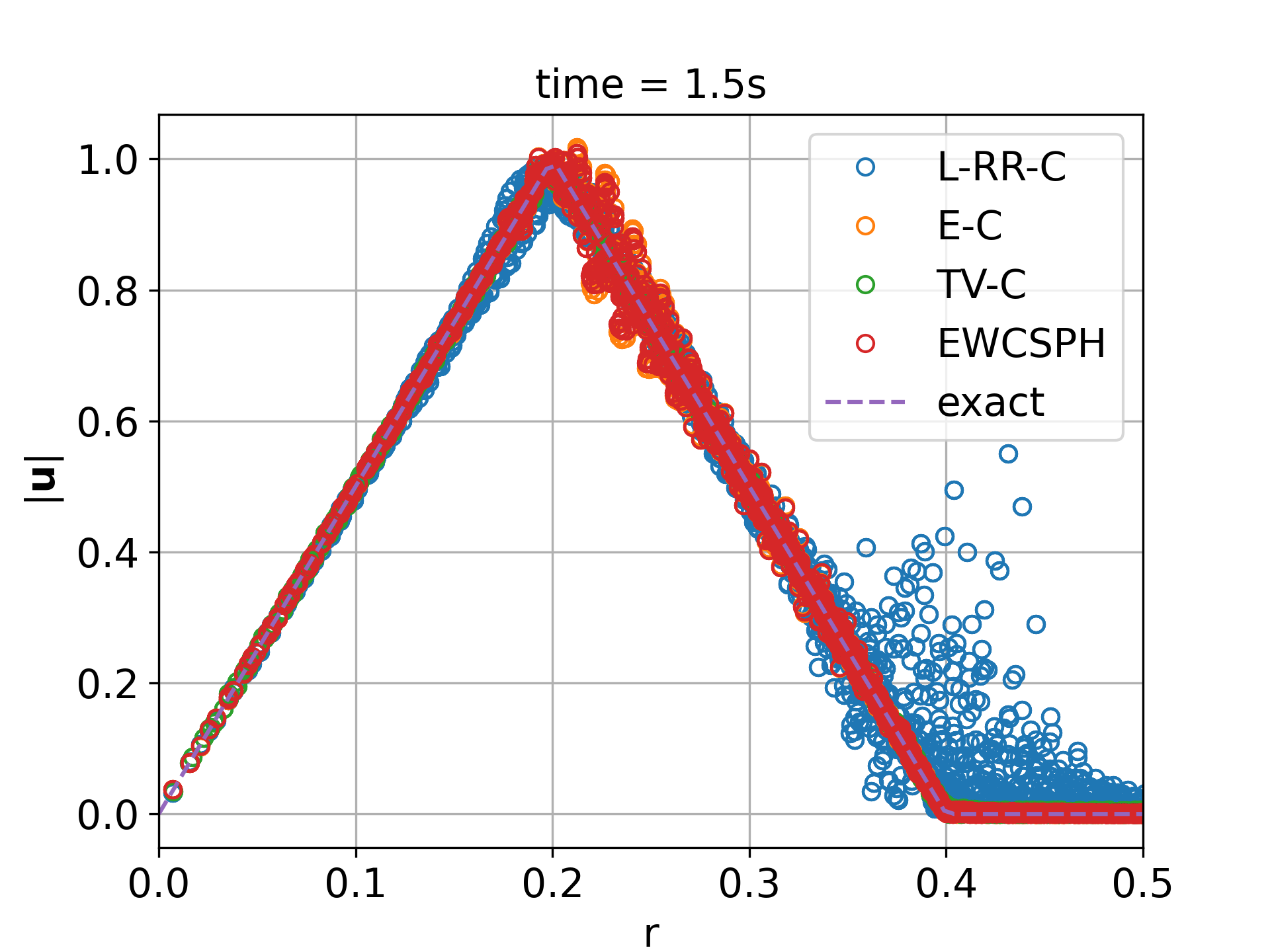
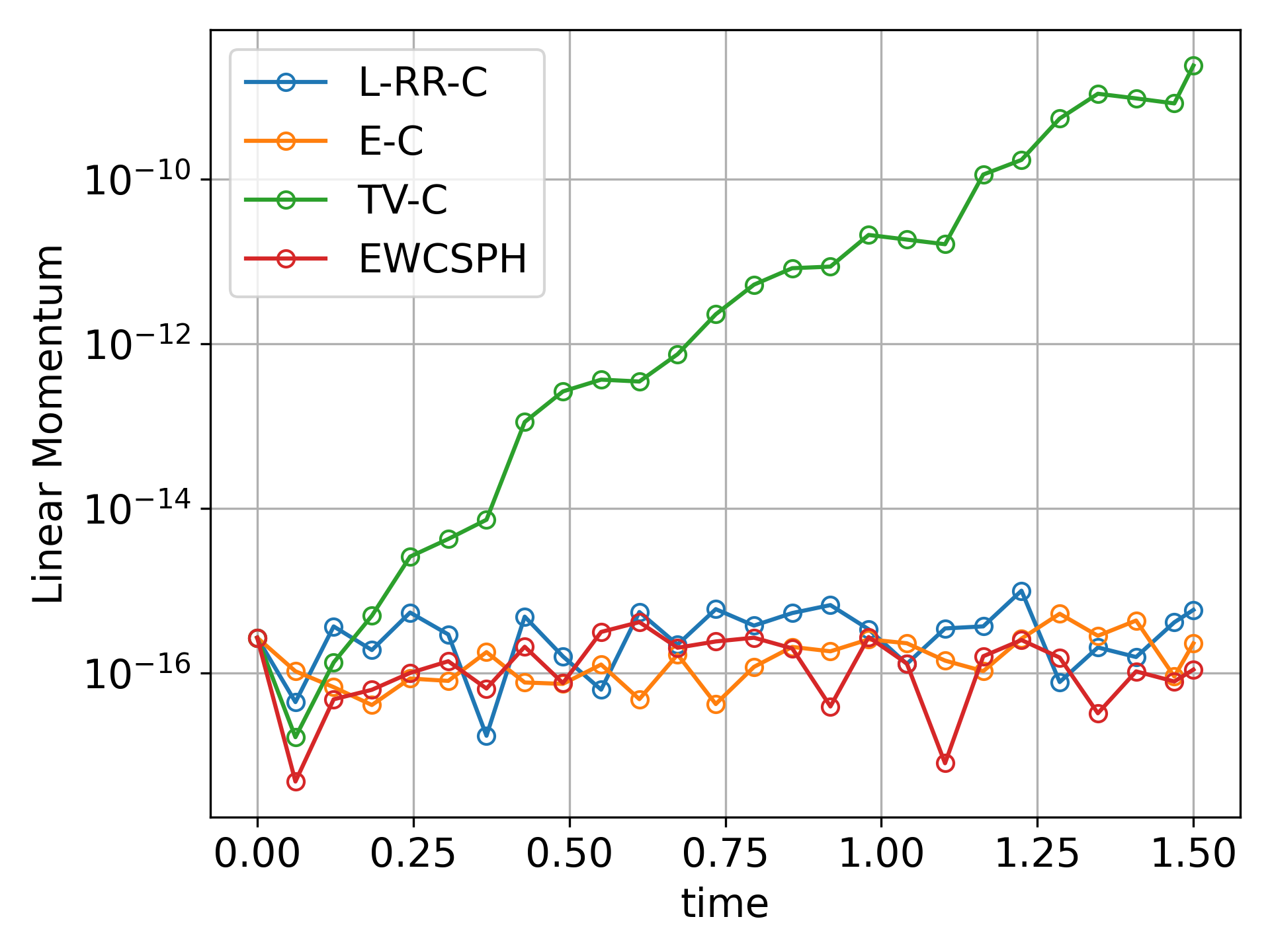
Figure 25: The velocity of particles with the distance from the center of the vortex (left) and the $x$-component of the total linear momentum (right) for the Gresho-Chan vortex problem.

In this section, we show the results for the scheme for which the Gresho-Chan vortex problem failed to complete. In fig. 25, we plot the velocity of the particles with the distance, $r$ from the center at $t=1.5s$, and the linear momentum in the x-direction with time for a $100\times 100$ simulation. Clearly, all the schemes considered show better approximate conservation of linear momentum compared to other scheme; however, they fail to complete.

In case of L-RR-C, due to the present of sharp change in the velocity field, the remeshing procedure diverges Chaniotis, Poulikakos, and Koumoutsakos (2002). In case of E-C, TV-C and EWCSPH, we suspect that the advection term $\mathbf{u}\cdot\nabla\mathbf{u}$ (or $\delta\mathbf{u}\cdot\nabla\mathbf{u}$ in case of TV-C) diverge in the absence of viscosity. This opens possible avenues of research to obtain a better discretization of the advection term.

References

- Monaghan (1994) J. J. Monaghan, “Simulating free surface flows with SPH,” Journal of Computational Physics 110, 399–406 (1994).
- Vacondio et al. (2020) R. Vacondio, C. Altomare, M. De Leffe, X. Hu, D. Le Touzé, S. Lind, J.-C. Marongiu, S. Marrone, B. D. Rogers, and A. Souto-Iglesias, “Grand challenges for Smoothed Particle Hydrodynamics numerical schemes,” Computational Particle Mechanics (2020), 10.1007/s40571-020-00354-1.
- Hernquist and Katz (1989) L. Hernquist and N. Katz, “TREESPH-A unification of SPH with the hierarchical tree method,” The Astrophysical Journal Supplement Series 70, 419–446 (1989).
- Quinlan, Basa, and Lastiwka (2006) N. J. Quinlan, M. Basa, and M. Lastiwka, “Truncation error in mesh-free particle methods,” International Journal for Numerical Methods in Engineering 66, 2064–2085 (2006).
- Zhu, Hernquist, and Li (2015) Q. Zhu, L. Hernquist, and Y. Li, “Numerical convergence in smoothed particle hydrodynamics,” The Astrophysical Journal 800, 6 (2015).