Contact Angle of an Evaporating Droplet of Binary Solution on a Super Wetting Surface

Abstract

We study the dynamics of contact angle of a droplet of binary solution evaporating on a super wetting surface. Recent experiments show that although equilibrium contact angle of such droplet is zero, the contract angle can show complex time dependence before reaching the equilibrium value. We analyse such phenomena by extending our previous theory for the dynamics of an evaporating single component droplet to double component droplet. We show that the time dependence of the contact angle can be quite complex. Typically, it first decreases slightly, and then increases and finally decreases again. Under certain conditions, we find that the contact angle remains constant over a certain period of time during evaporation. We study how the plateau or peak contact angle depends on the initial composition and the humidity. The theory explains experimental results reported previously.

I Introduction

Evaporation of liquid droplets is a phenomenon commonly seen in our daily life. It is also important in recent technologies, such as ink-jet printing [1, 2], nanopatterning depositions [3, 4, 5, 6, 7], and medical diagnostics [8, 9].

Evaporation of liquid droplets is a material transport problem in which the capillary flow of liquid is coupled with phase change and diffusion, and includes surprisingly complex problems of basic science. The complexity is seen in the simple case that a single component droplet is evaporating on a super-wetting surface. If the liquid is non-volatile and not evaporating, the droplet spreads on the surface, but if the liquid is evaporating, the droplet first spreads, but then recedes due to evaporation. It has been reported that in such situation, the contact angle often shows quasi-stationary, apparent contact angle $\theta_{app}$. The phenomena has been studied extensively by experiments and simulation [10, 11, 12, 13, 14, 15].

The evaporation behavior of droplets becomes even more complex for solutions [16, 17, 18, 19, 20, 21]. In solutions, the composition of the solution changes in time by evaporation, and therefore the physical parameters characterizing the fluid, such as viscosity, surface tension and the equilibrium contact angle change in time. This makes the time dependence of the contact angle complicated.

In a simple case, the time dependence of the contact angle can be understood by the composition change of the droplet due to the difference in the evaporation rate of each component. For example, in the ethanol/water mixture, the contact angle was observed to increase in time [22, 23, 24, 25, 26, 27] and this has been understood as the result of the enrichment of water which is less volatile and has larger contact angle than ethanol.

Recently, Cira et al. [28, 29] reported a phenomenon that cannot be explained by such simple reasoning. They measured the contact angle of a droplet of propylene glycol (PG)/water on a super-wetting glass substrate, where both pure PG and pure water droplet spreads completely. Since the equilibrium contact angles of both components are zero, one expects that the contact angle $\theta(t)$ will decrease monotonically in time. Unlike the expectation, they observed that $\theta(t)$ stays at a constant value in the first several minutes as if there is some apparent contact angle, or even increases in time, showing maximum, and finally starts to decrease to zero. Similar behavior has been reported by Li et al. [30] for the aqueous solution of 1,2-hexanediol. Karpitschka et al. [31] also reported that in water/carbon diol solution, the contact angle indeed remains at a constant value for an extended period of time before it starts to decrease.

Such anomalous time dependence of the contact angle has been considered to be caused by the Marangoni flow: since the water content at the droplet edge decreases quickly, the fluid flows from the edge region to the center due to the difference in the surface tension of water and PG. This opposes the spreading of the droplet and tends to increase the contact angle.

Theoretical study of such phenomena becomes complex since the fluid flow is coupled with the concentration field through the concentration dependence of the evaporation rate, and the surface tension. Diddens et al. [25, 26, 27] conducted a finite element simulation for the evaporation of multi-components droplets, accounting for the evaporation-induced Marangoni flow and thermal effects. Karpitschka et al. [31] studied the phenomena for 1,2-butanediole/water and found that the apparent contact angle $\theta_{\rm{app}}$ decreases with the increase of the relative humidity $RH$, satisfying the relation $\theta_{app}\sim\left(RH_{eq}-RH\right)^{1/3}$, and developed a scaling argument to explain the relation. Williams et al. [32] conducted more detailed analysis taking into account of the thermal Marangoni effect.

In such theoretical studies, the analysis was done by solving a set of non-linear pde (the convective diffusion equation taking into account of the Marangoni effect). Though one can do detailed modeling by including various effects, such analysis introduces many parameters in the theory, and makes it difficult to have overview or physical insight for the phenomena.

In this paper, we take a different approach. We assume that the droplet shape is a paraboloid, and derive time evolution equations for the parameters characterizing the profile, i.e., the contact radius $R(t)$ and contact angle $\theta(t)$ using Onsagers’s variational principle [33, 34, 35, 36, 37, 38, 39]. This work is an extension of our previous work for the droplet motion induced by surface tension gradient [40]. In the previous problem, the surface tension gradient is known. In the present problem, the surface tension gradient is not known and must be determined by the theory. In this paper, we shall reconstruct the previous theory by introducing a new variable, the concentration field of volatile component $C(r,t)$ ($r$ being the distance from the center), and derive a set of equations to determine their time evolution. The theory quantifies the existing argument for the Marangoni contraction of evaporating droplets, and predicts how the initial concentration and the evaporation condition affects the time evolution of the contact angle. The results explains the experimental results reported previously [28, 31, 29, 30].

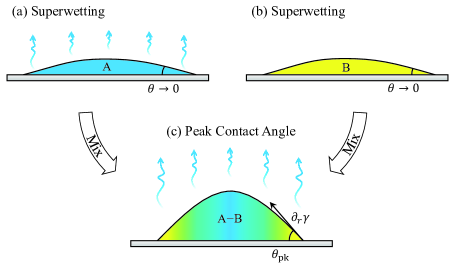
Figure 1: Schematic pictures of droplet with (a) single volatile component, (b) single nonvolatile component, and (c) mixture of the two components. Both of the two components are complete wetting on the substrate, and the surface tension of the volatile component is larger than the nonvolatile one. The evaporation of volatile component of the binary droplet in (c) causes an inward Marangoni flow, which induces a peak contact angle $\theta_{\rm{pk}}$ during evaporation.

II Theoretical Framework

We consider a two component droplet made of volatile component A and non-volatile component B, placed on a super wetting substrate (see Figure 1). We assume that the droplet contact angle is small and the surface profile is represented by a parabolic function,

$$h(r,t)=H(t)\left[1-\frac{r^{2}}{R^{2}(t)}\right],$$ (1)

where $H(t)$ is the height at the center and $R(t)$ is the radius of the droplet base. The droplet volume $V(t)$ is then given by,

$$V(t)=\frac{\pi}{2}H(t)R^{2}(t).$$ (2)

The contact angle $\theta(t)$ is given by $-\partial h(r,t)/\partial r$ at $r=R(t)$. Eqs. (1) and (2) then give,

$$\theta(t)=\frac{4V(t)}{\pi R^{3}(t)}.$$ (3)

The droplet volume changes due to evaporation. Let $J(r,t)$ be the evaporation rate (defined as the liquid volume evaporating to air per unit time per unit surface area) at point $r$ and time $t$. Then the volume change rate $\dot{V}(t)$ is given by

$$\dot{V}(t)=-\int_{0}^{R(t)}2\pi rJ(r,t)dr.$$ (4)

We assume that the solution is ideal, and use the following simple model for the evaporation rate $J(r,t)$ at point $r$ [27, 41, 42]

$$J(r,t)=J_{A}(t)[C(r,t)-RH],$$ (5)

where $C(r,t)$ is the molar fraction of the volatile component (the non-volatile component is assumed not to evaporate), $RH$ is the relative humidity and $J_{A}(t)$ is the evaporation rate for the hypothetical situation of $C(r,t)=1$ and $RH=0$, i.e., the situation that the droplet is made of pure A component and placed in the environment of zero humidity.

Due to the evaporation of the droplet itself, $RH$ in eq.(5) can be a function $r$, but we ignore this effect and assume that $RH$ is constant independent of position and time. Equation (5) indicates that evaporation takes place only when $C(r,t)>RH$. When $C(r,t)=RH$, there is no evaporation, and when $C(r,t)<RH$, $J(r,t)$ becomes negative and condensation takes place.

$J_{A}(t)$ in eq.(5) is inversely proportional to the droplet radius $R(t)$, and can be written as [41, 43, 39, 42]

$$J_{A}(t)=J_{A0}\frac{R_{0}}{R(t)}$$ (6)

where $J_{A0}$, and $R_{0}$ are the initial values of $J_{A}(t)$ and $R(t)$.

We define the characteristic time of evaporation $\tau_{\rm ev}$ by

$$\tau_{\rm{ev}}=-\frac{V_{0}}{\dot{V}_{0}}$$ (7)

Since $\dot{V}_{0}$ and $V_{0}$ are given by $\dot{V}_{0}=\pi R_{0}^{2}J_{A0}$ and $V_{0}=(\pi/4)\theta_{0}R_{0}^{3}$, $\tau_{\rm{ev}}$ is written as $\tau_{\rm{ev}}=4J_{A0}/\theta_{0}R_{0}$. Hence Eq.(5) is written as

$$J(r,t)=\frac{\theta_{0}R^{2}_{0}}{4\tau_{\rm ev}R(t)}[C(r,t)-RH].$$ (8)

The conservation equation for the liquid volume is written as,

$$\frac{\partial h}{\partial t}=-\frac{1}{r}\frac{\partial(rv_{f}h)}{\partial r}-J,$$ (9)

where $v_{f}(r)$ is the height averaged velocity of the fluid at point $r$.

By use of eq.( 1), the left hand side of Eq. (9) can be expressed by $\dot{R}$ and $\dot{V}$. Then Eq. (9) is solved for $v_{f}(r)$ (see Supplemental Material for details). This gives

$$v_{f}=r\frac{\dot{R}}{R}-\left(\frac{r}{2V}+\frac{r^{3}}{2\pi R^{4}h}\right)\dot{V}-\frac{1}{rh}\int_{0}^{r}r^{\prime}J(r^{\prime};t)dr^{\prime}.$$ (10)

The mass conservation equation for the volatile component is written as

$$\frac{\partial{\left(Ch\right)}}{\partial t}=-\frac{1}{r}\frac{\partial(rv_{f}Ch)}{\partial r}-J,$$ (11)

The first term on the right hand side represents the effect of convection, and the second term represents the evaporation. The effect of diffusion is ignored in the present theory, but its effect will be discussed later.

Combining Eqs. (9) and (11), we have the time derivative of $C(r,t)$,

$$\dot{C}=-v_{f}\frac{\partial C}{\partial r}-\frac{J}{h}\left(1-C\right).$$ (12)

This equation indicates explicitly that even if the initial composition of the droplet is uniform, the composition becomes non-uniform due to the evaporation of volatile component. Since $h(r,t)$ becomes zero at the contact line, Eq.(12) also indicates that at $r=R(t)$, $C(r,t)$ relaxes to the equilibrium value very quickly, and therefore $C(R(t),t)=RH$.

Careful inspection of the above set of equations indicates that there is only one unknown, $\dot{R}$, which we need to calculate to determine the time evolution of the system. This is seen as follows. Suppose that we know $V(t)$, $R(t)$ and $C(r,t)$ at time $t$, then $J(r,t)$ is given by Eq. (8) and $\dot{V}$ is given by Eq. (4). Hence $v_{f}(r)$ is expressed as a linear function of $\dot{R}$ by Eq. (10). Therefore if $\dot{R}$ is known, $\dot{C}$ is calculated by Eqs. (10) and (11). Therefore, the time evolution of $R(t)$, $V(t)$ and $C(r,t)$ can be calculated if $\dot{R}$ is known.

In the following, we shall use the Onsager variational principle [33, 34, 35, 36, 37, 38, 39, 40, 44, 45, 46, 47] to derive the equation for $\dot{R}(t)$. The calculation is essentially the same as that used in the previous paper [40] for the motion of an evaporating droplet under surface tension gradient. We consider the Rayleihian $\mathcal{R}$ defined by

$$\mathcal{R}=\Phi+\dot{F},$$ (13)

where $\Phi$ is the energy dissipation function, and $\dot{F}$ is the free energy time change rate. We obtain $\mathcal{R}$ as a function of $\dot{R}$, and obtain $\dot{R}$ by the condition $\partial\mathcal{R}/\partial\dot{R}=0$.

The energy dissipation is caused by the fluid flow inside the droplet and $\Phi$ is written as [40],

$$\Phi=\int_{0}^{R}2\pi r\frac{\eta}{2h}\left[12\left(v_{f}-\frac{v_{s}}{2}\right)^{2}+v_{s}^{2}\right]dr,$$ (14)

where $\eta$ is the viscosity of the fluid, which is assumed to be constant, and $v_{s}(r)$ is the fluid velocity at the liquid-vapor interface. In Eq. (14), we have ignored the extra friction associated with the contact line motion (i.e., the contact line friction coefficient $\xi_{\rm{cl}}$ [39] has been set to zero.)

The interfacial free energy of the system is given by

$$F=\int_{0}^{R}2\pi rdr\left[\gamma(r)\left(1+\frac{1}{2}h^{\prime 2}\right)-\gamma_{A}\cos\theta_{eA}\right],$$ (15)

where $\theta_{eA}$ is the equilibrium contact angle for A component, and $\gamma(r)$ is the surface tension of the solution at point $r$. We assume a linear dependence of $\gamma(r)$ on $C(r)$ [42],

$$\gamma(r)=C(r)\gamma_{A}+\left[1-C(r)\right]\gamma_{B},$$ (16)

where $\gamma_{A}$ and $\gamma_{B}$ are the surface tensions of pure $A$ and $B$ components.

The dissipation function $\Phi$ involves the surface velocity $v_{s}(r)$, but this is expressed by $v_{f}(r)$ and the surface tension gradient $\partial\gamma/\partial r$ (see Supplemental Material).

$$v_{s}=\frac{3v_{f}}{2}+\frac{h}{4\eta}\frac{\partial\gamma}{\partial r}.$$ (17)

By use of Eqs. (10) and (17) in Eq. (14), the Rayleighian can be expressed as a quadratic function of $\dot{R}$. Therefore the time evolution for $R(t)$ is determined by the condition $\partial\mathcal{R}/\partial\dot{R}=0$. The calculation is straightforward, but cumbersome, and described in the Supplemental Material. In the end, we obtain the following equation for $\dot{R}$

$$\begin{aligned} \dot{R}=&\frac{\left(\gamma_{\rm{re}}-1\right)\theta V_{0}^{\frac{1}{3}}}{3\gamma_{\rm{re}}\alpha\tau_{\rm{re}}}\left[\int_{0}^{R}C\frac{r}{R^{2}}\left(\frac{2r^{2}\theta^{2}}{R^{2}}-5\right)dr+\frac{\theta^{2}-\gamma_{\rm{re}}\theta_{\rm eA}^{2}}{2\left(\gamma_{\rm{re}}-1\right)}+\frac{3}{2}C\left(R\right)+1\right]-\frac{R\dot{V}}{4\alpha V}\\ -&\frac{\theta\theta_{0}R_{0}^{2}}{4\alpha R^{3}\tau_{\rm{ev}}}\int_{0}^{R}\frac{r}{h^{2}}\left[\int_{r}^{R}r^{\prime}\left(C-RH\right)dr^{\prime}\right]dr,\end{aligned}$$ (18)

where $\gamma_{\rm{re}}=\gamma_{A}/\gamma_{B}$ is the surface tension ratio of the two components, $\alpha=\ln(R/2\epsilon)-1$ is a parameter which is regarded as constant in the subsequent analysis, $\epsilon$ is the molecular cutoff length, and $\tau_{\rm{re}}$ is defined by

$$\tau_{\rm{re}}=\eta V_{0}^{1/3}/\gamma_{A}$$ (19)

which represents the characteristic relaxation time of the droplet determined by viscosity $\eta$ and the surface tension $\gamma_{A}$.

Since $\dot{\theta}$ is related to $\dot{V}$ by (see Eq. (3)),

$$\dot{\theta} =\frac{\theta\dot{V}}{V}-\frac{3\theta\dot{R}}{R}.$$ (20)

Eq. (18) gives the following equation for $\dot{\theta}$,

$$\begin{aligned} \dot{\theta}=&\frac{\left(\gamma_{\rm{re}}-1\right)\theta^{2}V_{0}^{\frac{1}{3}}}{\gamma_{\rm{re}}\alpha\tau_{\rm{re}}R}\left[\int_{0}^{R}C\frac{r}{R^{2}}\left(5-\frac{2r^{2}\theta^{2}}{R^{2}}\right)dr-\frac{\theta^{2}-\gamma_{\rm{re}}\theta_{\rm eA}^{2}}{2\left(\gamma_{\rm{re}}-1\right)}-\frac{3}{2}C\left(R\right)-1\right]\\ +&\frac{\theta\dot{V}}{V}\left(1+\frac{3}{4\alpha}\right)+\frac{3\theta^{2}\theta_{0}R_{0}^{2}}{4\alpha R^{4}\tau_{\rm ev}}\int_{0}^{R}\frac{r}{h^{2}}\left[\int_{r}^{R}r^{\prime}\left(C-RH\right)dr^{\prime}\right]dr.\end{aligned}$$ (21)

To summarize, the time evolution of the system can be calculated as follows. The non-equilibrium state of the system is specified by three variables $\theta(t)$ and $V(t)$ and $C(r,t)$. Their time derivatives are calculated as follows.

• $\dot{V}$ is calculated by Eq. (4), where $J(r,t)$ is given by Eq. (5).

• $\dot{\theta}$ and $\dot{R}$ are given by Eq. (21) and Eq. (20)

• $\dot{C}$ is given by Eq. (12), where $v_{f}$ is given by Eq. (10)

Since they are a set of ordinary and first order partial differential equations, the calculation is simple and quick. We shall show the results in the next section.

The above time evolution equations become simple for the special case of pure liquid (i.e., the case of $C=1$). In this case, taking $\theta_{\rm eA}=0$ they reduce to the following equations (see Supplemental Material),

$$\dot{R} = \frac{V_{0}^{1/3}}{6\alpha\tau_{re}}\theta^{3}+\frac{R}{4V}\dot{V}$$ (22)

$$\dot{\theta} = -\frac{V_{0}^{1/3}}{2\alpha\tau_{re}}\theta^{4}+\frac{\theta}{4V}\dot{V}$$ (23)

The first terms on the right hand side of Eqs. (22) and (23) represent the Tanner’s law [48, 49] for spreading, and the second terms represents the effect of liquid evaporation. These equations agree with the previous results [39]. Equation (23) indicates that $\dot{\theta}$ is always negative for pure liquid droplet. This conclusion is not consistent with the recent works [50, 51] which claim that $\dot{\theta}$ become zero in a certain range of time if the droplet is evaporating. The discrepancy can be resolved by taking into account of the non-uniform evaporation rate in pure liquid droplet. Detailed discussion will be given in a future article.

III Results and Discussions

Since there are many parameters involved in Eq. (21), we focus on two parameters which can be changed easily in experiments, the initial composition of the volatile component $C_{0}$, and the humidity $RH$. In the following we study the time evolution of $\theta(t)$ and $R(t)$ by changing the two parameters while keeping the other parameters fixed as follows; initial contact angle $\theta_{0}=0.3$, surface tension ratio $\gamma_{\rm{re}}=\gamma_{A}/\gamma_{B}=2$, equilibrium contact angles $\theta_{\rm eA}=\theta_{\rm eB}=0$. With such set up, the subsequent discussion is limited to the case that the surface tension of volatile component is larger than the non-volatile component (i.e., the case of $\gamma_{\rm{re}}>1$), but the opposite case of $\gamma_{\rm re}<1$ can be studied by the present theory and is discussed in Supplemental Material.

III.1 Effect of initial composition $C_{0}$

Figure 2 shows the time variation of the contact angle $\theta(t)$ and the contact radius $R(t)$ for various initial concentration $C_{0}$ of volatile component.

The curves of $C_{0}=0.3$ correspond to the case of non-evaporating droplet since the flux $J$ in Eq. (5) becomes zero at this concentration. In this case, the droplet keeps uniform composition and behaves as a non-volatile liquid. Its dynamics is described by Eqs. (22) and (23) with $\dot{V}=0$. Hence, $R(t)$ increases in time and $\theta(t)$ decreases in time.

The curves of $C_{0}=1.0$ correspond to the case of pure evaporating droplet and its dynamics is again described by Eqs. (22) and (23). In the case of Figure 2 (a) and (b), both $\theta(t)$ and $R(t)$ decrease to zero monotonically. The monotonic decrease of $\theta(t)$ is a general result of the present theory for pure liquid, but the monotonic decrease of $R(t)$ is a result of the choice of the initial condition. (The figure shows the result of the case of $\theta_{0}=0.3$. If $\theta_{0}$ is larger, $R(t)$ first increases in time and then starts to decrease.)

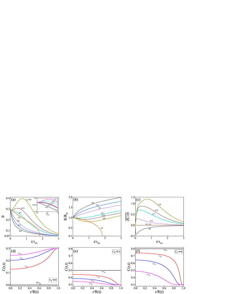
Figure 2: Evolution of (a) droplet contact angle $\theta(t)$, (b) droplet contact radius $R(t)/R_{0}$, and (c) average concentration gradient $\overline{\partial C/\partial r}$ of an evaporating binary droplet for various initial concentration of volatile component, $C_{0}$. The inset figure in (a) is the zoom in evolution of the contact angle, indicating that the peak contact angle changes to quasi-stationary (or apparent) contact angle for a short time interval by decreasing $C_{0}$ ($C_{0}=0.72$ and $0.71$). (d), (e), and (f) show the concentration distribution in the droplet at different times for three initial concentration (d) $C_{0}=0.0$, (e) $C_{0}=0.5$, and (f) $C_{0}=0.8$. In all cases, $k_{\rm{ev}}=0.002$, and $RH=0.3$.

The droplets having initial concentration $C_{0}$ between 0.3 and 1, show the effect of Marangoni contraction. As it is seen in Figure 2 (e) and (f), $C(r,t)$ decreases quickly to the equilibrium value $0.3$ at the edge of the droplet, while $C(r,t)$ at the center is larger than this value. This concentration gradient creates surface tension gradient in the droplet, and causes an inward Marangoni flow from the edge to the center. Such inward flow suppresses the decrease of $\theta(t)$, and creates the plateau-like region in the plot of $\theta(t)$. The inset of Figure 2 (a) shows such plateau region for $C_{0}$, $0.7<C_{0}<0.72$. With further increase of $C_{0}$, $\theta(t)$ shows a peak.

Although the present theory accounts for the effect of Marangoni contraction, it does not give a clear plateau behaviour for $\theta(t)$: the plateau appears only in a limited time range or limited parameter space. It is difficult to identify the “apparent contact angle” in our result. We therefore focused on the peak of the contact angle since it represents the anomalous time dependence of $\theta(t)$, and corresponds to the height of the plateau when $\theta(t)$ shows the plateau. Cira also reported that the quasi-stationary contact angle is observed in a limited parameter space [28].

The anomaly in the contact angle is caused by the concentration gradient created in the binary droplet by evaporation. The relation between the concentration gradient and the peak contact angle is seen in Figure 2 (c), where the average concentration gradient

$$\overline{\frac{\partial C}{\partial r}}=\frac{2}{R^{2}}\int_{0}^{R}drr\frac{\partial C}{\partial r}$$ (24)

is plotted against time. It is seen that $\overline{\partial C/\partial r}$ has a peak, and that the peak time of $\overline{\partial C/\partial r}$ is close to the peak time of $\theta(t)$. This again supports the mechanism of the contact angle anomaly in binary droplet.

If the initial concentration $C_{0}$ is smaller than the equilibrium value 0.3, condensation takes place instead of evaporation. It is interesting to see that there is no anomaly in the behavior of $\theta(t)$ and $R(t)$: their behaviour are quite continuous across this boundary from evaporation to condensation.

III.2 Effects of humidity

Figure 3 shows the effect of humidity $RH$ on the time evolution of the droplet having initial composition $C_{0}=0.6$. The effect of humidity $RH$ is qualitatively similar to the effect of initial composition $C_{0}$. When humidity is high ($RH=0.6$), there is no evaporation, and the droplet spreads on the surface as a non-volatile liquid, showing monotonous decrease of $\theta(t)$ and monotonous increase of $R(t)$. With the decrease of $RH$, evaporation starts, and the effect of Marangoni contraction sets in. Accordingly $\theta(t)$ starts to show a plateau or a peak. The time evolution of the average concentration gradient (Figure 3(c)) and the time evolution of the concentration profile (Figure 3 (d) and (e) ) confirms that the same mechanism is working as in the case of Figure 2.

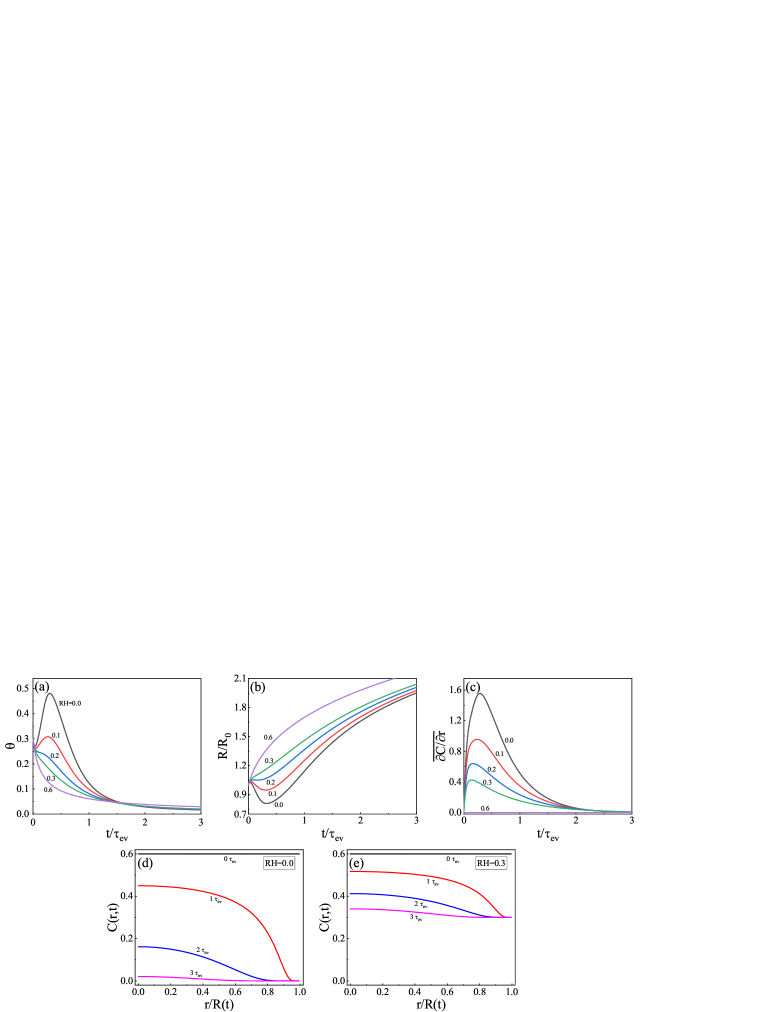
Figure 3: (a) Time dependence of (a) the contact angle $\theta(t)$, (b) the contact radius $R(t)/R_{0}$, and (c) the averaged concentration gradient of the volatile component for various relative humidity $RH$. The evolution of the distribution of volatile component concentration within the droplet for (d) $RH=0.0$, and (e) $RH=0.3$. In all cases, $C_{0}=0.6$, and $k_{\rm ev}=5\times 10^{-4}$.

III.3 Peak contact angle

As it has been shown in previous sections, the contact angle $\theta(t)$ shows a peak $\theta_{\rm{pk}}$ when the evaporation is strong (i.e., when the initial concentration $C_{0}$ is large or when the humidity $RH$ is small). Figure 4 (a) shows the plot of the peak contact angle $\theta_{\rm{pk}}$ against the initial concentration $C_{0}$. Figure 4 (b) shows the plot of $\theta_{\rm{pk}}$ against the average concentration $\bar{C}=2\int_{0}^{R}Cr/R^{2}dr$ when the peak appears.

In order to understand the behavior shown in Figure 4 (b), we evaluate the integral on the right hand side of Eq. (21) by replacing $C(r)$ with the average value $\bar{C}$. We also assume that $C(R)=RH$. This approximation gives the following equation for $\dot{\theta}$.

$$\tau_{\rm{ev}}\dot{\theta}=\frac{\left(\gamma_{\rm{re}}-1\right)\theta^{2}V_{0}^{\frac{1}{3}}}{\gamma_{\rm{re}}\alpha k_{\rm{ev}}R}\left[\bar{C}\left(\frac{5}{2}-\frac{\theta^{2}}{2}\right)-\frac{\theta^{2}-\gamma_{\rm{re}}\theta_{eA}^{2}}{2\left(\gamma_{\rm{re}}-1\right)}-\frac{3}{2}RH-1\right]+\frac{\theta\dot{V}\tau_{\rm{ev}}}{4V}$$ (25)

At the peak position, $\dot{\theta}$ is equal to zero. To simplify the equation further, we consider the limit of $k_{\rm{ev}}\rightarrow 0$. Then Eq. (25) is simplified as

$$\bar{C}\left(\frac{5}{2}-\frac{\theta_{\rm{pk}}^{2}}{2}\right)-\frac{\theta_{\rm{pk}}^{2}-\gamma_{\rm{re}}\theta_{eA}^{2}}{2\left(\gamma_{\rm{re}}-1\right)}-\frac{3}{2}RH-1=0.$$ (26)

Equation (26) is solved for $\theta_{\rm{pk}}$ as

$$\theta_{\rm{pk}} = \left[\frac{(\gamma_{\rm{re}}-1)(5\bar{C}-3RH-2)+\gamma_{\rm{re}}\theta_{eA}^{2}}{1+\left(\gamma_{\rm{re}}-1\right)\bar{C}}\right]^{\frac{1}{2}}$$ (27)

$$= \left[\frac{(\gamma_{A}-\gamma_{B})(5\bar{C}_{A}-3RH-2)+\gamma_{A}\theta_{eA}^{2}}{\gamma_{A}\bar{C}_{A}+\gamma_{B}\bar{C}_{B}}\right]^{\frac{1}{2}}.$$ (28)

where $\bar{C}_{A}$ and $\bar{C}_{B}$ stand for $\bar{C}$ and $1-\bar{C}$.

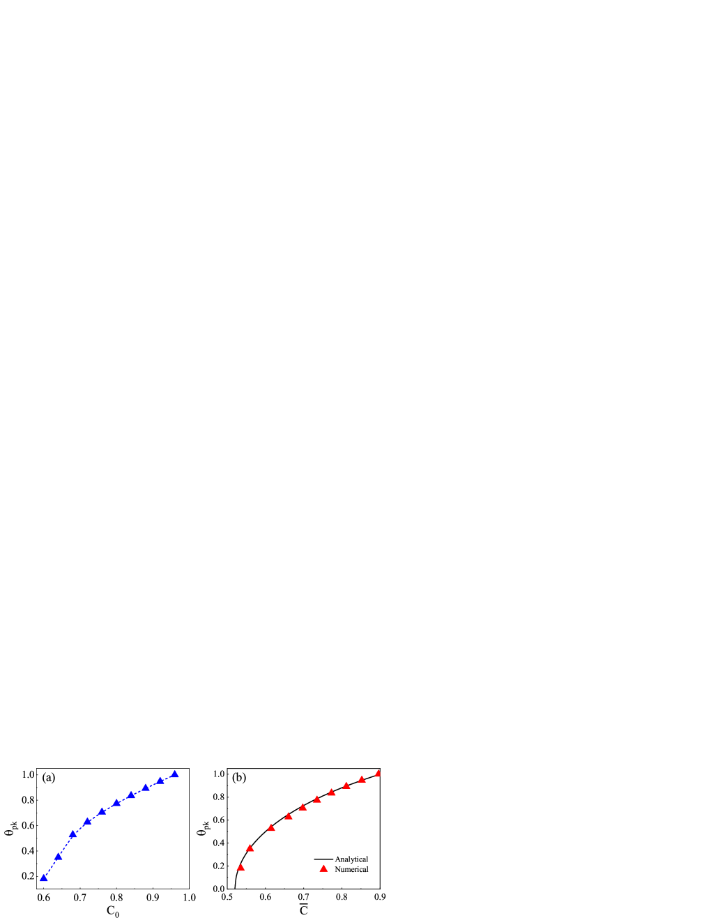
Figure 4: (a) The dependence of the peak contact angle $\theta_{\rm{pk}}$ on the initial concentration of volatile A-component, $C_{0}$. (b) The dependence of $\theta_{\rm{pk}}$ on $\bar{C}$, where $\bar{C}$ is the average concentration at the moment when $\theta_{\rm{pk}}$ occurs, $\bar{C}=2\int_{0}^{R}Cr/R^{2}dr$. The results obtained from the full numerical calculations are denoted by symbols, while the analytical result is denoted by the black-solid line. All the other parameters are $k_{\rm ev}=1\times 10^{-4}$, and $RH=0.2$. .

We compare the value of $\theta_{\rm{pk}}$ calculated by Eq. (28) with that obtained by the full numerical calculation in Figure 4(b) for $RH=0.2$. It is seen that the result of Eq. (28) (solid line) agrees quite well with that of the full numerical calculation (data points).

Equation (28) indicates that for the peak (or plateau) to be observed, $5\bar{C}-3RH-2$ must be positive. Since $\bar{C}$ is smaller than $C_{0}$, this condition indicates that $5C_{0}-3RH-2$ must be positive for the peak to be observed. In other word, for the peak (or plateau) to be observed the initial condition must satisfy

$$C_{0}>\frac{3RH+2}{5}$$ (29)

Such condition is consistent with the behaviour of $\theta(t)$ shown in Figure 2. It is interesting to check the prediction by experiments.

Equation (28) is useful to estimate the value of $\theta_{\rm{pk}}$. Since $\bar{C}$ at the peak position is not very different from the initial concentration $C_{0}$, $\theta_{\rm{pk}}$ can be estimated by Eq. (28) with $\bar{C}$ replaced by $C_{0}$.

Equation (28) also indicates that $\theta_{\rm pk}$ depends on $RH$ in the form of $\theta_{\rm pk}\simeq(RH_{eq}-RH)^{1/2}$. This relation has been confirmed by our full numerical calculations as it is shown in Figure 5. The relation is also qualitatively consistent with the previous experimental results. Karpitschka et al. [31] reported that the apparent contact angle $\theta_{app}$ decreases with $RH$ following the relation $(RH_{eq}–RH)^{1/3}$. Cira et al. [28] found a linear relation between $\cos\theta_{app}$ and $RH$, which is equivalent to $\theta_{app}\propto(RH_{eq}–RH)^{1/2}$. When $\theta_{\rm pk}$ meets the valley contact angle $\theta_{\rm vl}$, a plateau of the contact angle appears.

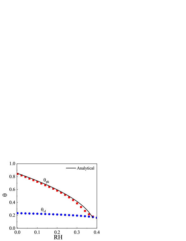
Figure 5: The dependence of the peak contact angle $\theta_{\rm{pk}}$ and the valley contact angle $\theta_{\rm{vl}}$ on the relative humidity of volatile A-component, $RH$. Symbols denote the results of the full numerical calculations. The black-solid line denotes the analytical results of Eq. (27), where we take $\bar{C}=0.637$ and $\theta_{\rm eA}=0$. Here the value of $\bar{C}$ is the average of $\bar{C}$ when $\theta_{pk}$ occurs for different $RH$. In all cases, $k_{ev}=1\times 10^{-4}$, and $C_{0}=0.7$.

IV Conclusion

In this paper, we developed a theory for the spreading dynamics of an evaporating droplet made of volatile and nonvolatile components. We have shown that in such two component liquid, the evaporation makes the time variation of the contact angle $\theta(t)$ and contact radius $R(t)$ quite complex since evaporation of the volatile component makes the concentration in the droplet non-uniform, and creates a Marangoni flow in the droplet. Here we limited our discussion to the case that the surface tension of the volatile component is larger than that of non-volatile component. We also limited the discussion that the equilibrium contact angles of both components are zero (super wetting surface). In such a case, the induced Marangoni flow is directed inward (from the edge to the center), which tends to decrease the contact radius and to increase the contact angle.

Using the Onsager principle, we derived a set of equations which determine the time evolution of the contact angle $\theta(t)$, contact radius $R(t)$ and concentration of volatile component $C(r,t)$. To derive the equation, we assumed

• The droplet has a profile of parabola, characterized by $R(t)$ and $\theta(t)$.

• The liquid is an ideal solution of A/B mixture, and the evaporation rate is given by Eq. (5)

Assumption (1) is needed to describe the spreading dynamics by two parameters $\theta(t)$ and $R(t)$, and assumption (2) is needed to introduce the effect of evaporation. Although the parabola assumption of the droplet surface profile can reveal a few features of drying droplets, it should be noticed that complicated shape of surface profile appears of drying droplets. Then, the full hydrodynamic equations are needed for the study of such cases.

There are other assumptions and approximations in the theory, such as the ignorance of diffusion and thermal effect. Diffusion decreases the concentration gradient and weaken the Marangoni flow. The effect of diffusion can be estimated by the Péclet number $Pe=v_{f}R/D$, where $v_{f}$ is the fluid velocity, $R$ is the contact radius, and $D$ is the mutual diffusion constant of water and oil. Taking the value of $v_{f}=2.1\times 10^{-6}~{}{\rm m/s}$, $R=2.5\times 10^{-3}~{}{\rm m}$ and $D=5.0\times 10^{-10}~{}{\rm m^{2}/s}$, $Pe$ is around 10. Therefore the diffusion is not entirely negligible, but it will not affect the present results seriously.

We emphasize that despite such approximations, the present theory explains the experimental observation that the plateau (or peak) contact angle appears only when the composition of the volatile component in the droplet is large enough, and that the value decreases with the increase of room humidity approximately in proportional to $(RH_{eq}-RH)^{1/2}$ [28]. Moreover, for the cases of $\gamma_{\rm re}<1$ that the surface tension of the faster evaporation component being smaller than the slower one [32], the enhanced droplet spreading by increasing the initial concentration of volatile component are captured by our model.

Acknowledgement.   We thank N. J. Cira for useful discussions. This work was supported by the National Natural Science Foundation of China (Grant No. 21822302), the joint NSFC-ISF Research Program, China (Grant No. 21961142020), and the Fundamental Research Funds for the Central Universities, China.

References

- [1] A. K. Thokchom, Q. Zhou, D.-J. Kim, D. Ha and T. Kim, Sens. Actuator B-Chem., 2017, , 1063-1070.
- [2] Y.-H. Kim, B. Yoo, J. E. Anthony and S. K. Park, Adv. Mater., 2012, , 497-502.
- [3] B. G. Prevo and O. D. Velev, Langmuir, 2004, , 2099-2107.
- [4] J. Park and J. Moon, Langmuir, 2006, , 3506-3513.
- [5] D. J. Harris and J. A. Lewis, Langmuir, 2008, , 3681-3685.
- [6] A. Yella, M. N. Tahir, S. Meuer, R. Zentel, R. Berger, M. Panthöfer and W. Tremel, J. Am. Chem. Soc., 2009, , 17566-17575.
- [7] Y. Wang, Y. Song, S. Watanabe, S. Zhang, D. Li and X. Zhang, ACS Appl. Mater. Interfaces, 2012, , 6443-6449.
- [8] T. A. Yakhno, V. G. Yakhno, A. G. Sanin, O. A. Sanina, A. S. Pelyushenko, N. A. Egorova, I. G. Terentiev, S. V. Smetanina, O. V. Korochkina and E. V. Yashukova, IEEE Eng. Med. Biol. Mag., 2005, , 96-104.
- [9] Y. J. P. Carreón, M. Ríos-Ramírez, R. E. Moctezuma and J. González-Gutiérrez, Sci. Rep., 2018, , 9580.
- [10] R.G. Picknett and R. Bexon, J. Colloid Interface Sci., 1977, , 336-350.
- [11] C. Bourgès-Monnier and M. E. R. Shanahan, Langmuir, 1995, , 2820-2829.
- [12] H. Y. Erbil, G. McHale and M. I. Newton, Langmuir, 2002, , 2636-2641.
- [13] J. M. Stauber, S. K. Wilson, B. R. Duffy and K. Sefiane, J. Fluid Mech., 2014, , R2.
- [14] J. M. Stauber, S. K. Wilson and B. R. Duffy, Langmuir, 2015, , 3653-3660.
- [15] V. Shrikanth, S. Archana and M. S. Bobji, Meas. Sci. Technol., 2019, , 075002.
- [16] J. R. E. Christy, Y. Hamamoto and K. Sefiane, Phys. Rev. Lett., 2011, , 205701.
- [17] R. Bennacer and K. Sefiane, J. Fluid Mech., 2014, , 649-665.
- [18] H. Kim and H. A. Stone, J. Fluid Mech., 2018, , 769-783.
- [19] A. M. J. Edwards, P. S. Atkinson, C. S. Cheung, H. Liang, D. J. Fairhurst and F. F. Ouali, Phys. Rev. Lett., 2018, , 184501.
- [20] M. A. Hack, W. Kwieciński, O. Ramírez-Soto, T. Segers, S. Karpitschka, E. S. Kooij and J. H. Snoeijer, Langmuir, 2021, , 3605-3611.
- [21] C. Diddens, Y. Li and D. Lohse, J. Fluid Mech., 2021, , A23.
- [22] K. Sefiane, L. Tadrist and M. Douglas, Int. J. Heat Mass Transf., 2003, , 4527-4534.
- [23] A. K. H. Cheng, D. M. Soolaman and H.-Z. Yu, J. Phys. Chem. B, 2006, , 11267-11271.
- [24] C. Liu, E. Bonaccurso and H.-J. Butt, Phys. Chem. Chem. Phys., 2008, , 7150-7157.
- [25] C. Diddens, J. Comput. Phys., 2017, , 670-687.
- [26] C. Diddens, H. Tan, P. Lv, M. Versluis, J. G. M. Kuerten, X. Zhang and D. Lohse, J. Fluid Mech., 2017, , 470-497.
- [27] C. Diddens, J. G. M. Kuerten, C. W. M. van der Geld and H. M. A. Wijshoff, J. Colloid Interface Sci., 2017, , 426-436.
- [28] N. J. Cira, A. Benusiglio and M. Prakash, Nature, 2015, , 446-450.
- [29] A. Benusiglio, N. J. Cira and M. Prakash, Soft Matter, 2018, , 7724-7730.
- [30] Y. Li, P. Lv, C. Diddens, H. Tan, H. Wijshoff, M. Versluis and D. Lohse, Phys. Rev. Lett., 2018, , 224501.
- [31] S. Karpitschka, F. Liebig and H. Riegler, Langmuir, 2017, , 4682-4687.
- [32] A. G. L.Williams, G. Karapetsas, D. Mamalis, K. Sefiane, O. K. Matar and P. Valluri, J. Fluid Mech., 2021, , A22.
- [33] L. Onsager, Phys. Rev., 1931, , 405-426.
- [34] L. Onsager, Phys. Rev., 1931, , 2265-2279.
- [35] M. Doi, Soft Matter Physics, Oxford University Press, 2013.
- [36] M. Doi, Chin. Phys. B, 2015, , 24, 020505.
- [37] M. Doi, Prog. Polym. Sci., 2021, , 101339.
- [38] X. Xu, U. Thiele and T. Qian, J. Phys. Condens. Matter, 2015, , 085005.
- [39] X. K. Man and M. Doi, Phys. Rev. Lett., 2016, , 066101.
- [40] X. K. Man and M. Doi, Phys. Rev. Lett., 2017, , 044502.
- [41] F. Parisse and C. Allain, Langmuir, 1997, , 3598-3602.
- [42] A. D. Eales, N. Dartnell, S. Goddard and A. F. Routh, J. Fluid Mech., 2016, , 200-232.
- [43] M. Kobayashi, M. Makino, T. Okuzono and M. Doi, J. Phys. Soc. Jpn., 2010, , 044802.
- [44] M. M. Wu, X. K. Man and M. Doi, Langmuir, 2018, , 9572-9578.
- [45] M. M. Wu, Y. N. Di, X. K. Man and M. Doi, Langmuir, 2019, , 2019, 14734-14741.
- [46] Z. C. Jiang, X. Y. Yang, M. M. Wu and X. K. Man, Chin. Phys. B, 2020, , 096803.
- [47] X. Y. Yang, Z. C. Jiang, P. H. Lyu, Z. Y. Ding and X. K. Man, Commun. Theor. Phys., 2021, , 047601.
- [48] L. H. Tanner, J. Phys. D: Appl. Phys., 1979, , 1473-1484.
- [49] A. Oron, S. H. Davis and S. G. Bankoff, Rev. Mod. Phys., 1997, , 931-980.
- [50] E. Jambon-Puillet, O. Carrier, N. Shahidzadeh, D. Brutin, J. Eggers and D. Bonn, J. Fluid Mech., 2018, , 817-830.
- [51] J. Eggers and L. M. Pismen, Phys. Fluids , 2010, , 112101.