X-GGM: Graph Generative Modeling for Out-of-Distribution Generalization in Visual Question Answering

Abstract.

Encouraging progress has been made towards Visual Question Answering (VQA) in recent years, but it is still challenging to enable VQA models to adaptively generalize to out-of-distribution (OOD) samples. Intuitively, recompositions of existing visual concepts (, attributes and objects) can generate unseen compositions in the training set, which will promote VQA models to generalize to OOD samples. In this paper, we formulate OOD generalization in VQA as a compositional generalization problem and propose a graph generative modeling-based training scheme (X-GGM) to implicitly model the problem. X-GGM leverages graph generative modeling to iteratively generate a relation matrix and node representations for the predefined graph that utilizes attribute-object pairs as nodes. Furthermore, to alleviate the unstable training issue in graph generative modeling, we propose a gradient distribution consistency loss to constrain the data distribution with adversarial perturbations and the generated distribution. The baseline VQA model (LXMERT) trained with the X-GGM scheme achieves state-of-the-art OOD performance on two standard VQA OOD benchmarks, , VQA-CP v2 and GQA-OOD. Extensive ablation studies demonstrate the effectiveness of X-GGM components. Code is available at https://github.com/jingjing12110/x-ggm.

1. Introduction

Visual Question Answering (VQA) (Antol et al., 2015), answering questions conditioned on understanding the given image and question, is a task toward general AI (Teney et al., 2017). Although considerable progress has been made in VQA, most methods usually process similar data distributions between training and test sets. However, a good VQA model should be robust against answer distribution shift (Kervadec et al., 2020) and perform well on out-of-distribution (OOD) testing (Teney et al., 2020c), , evaluating the ability of the model to generalize beyond dataset-specific language biases (Agrawal et al., 2016; Zhang et al., 2016; Goyal et al., 2017; Agrawal et al., 2018). This paper focuses on OOD generalization in VQA, aiming to improve the OOD generalization ability of baseline VQA models while preserving their in-domain (ID) performance.

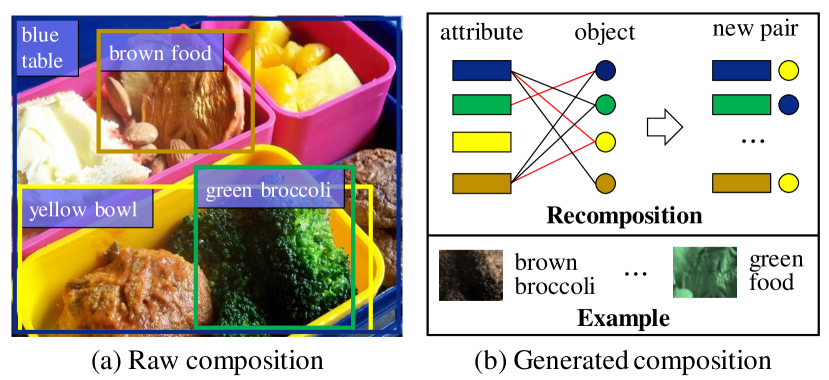
Figure 1. Compositional generalization implied in graph generative modeling. New compositions (, brown broccoli) of attributes and objects can be generated by raw compositions (, green broccoli and brown food).

Motivation

OOD generalization in VQA is challenging. To generalize to out-of-distribution samples adaptively, the VQA model should own two capabilities: (1) overcoming negative language biases and (2) producing out-of-distribution answers by learning rules entailed in in-domain data. The prevailing OOD generalization methods (Clark et al., 2019; Wu and Mooney, 2019; Gokhale et al., 2020; Clark et al., 2020) focus on enhancing the first capability, which achieves OOD generalization by explicitly mitigating the language biases. While the second capability, which directly endues VQA models the potentiality to generalize to out-of-distribution (, unseen or rare) samples, has not been well explored.

Benefiting from good compositional generalization capabilities, humans can easily achieve OOD generalization (Lake et al., 2017). Motivated by this, we formulate OOD generalization in VQA as a compositional generalization problem and leverage in-domain data to generate new/raw compositions of existing visual concepts (, attributes and objects) to make VQA models produce out-of-distribution answers. As shown in Figure 1, given any two attribute-object pairs, such as green broccoli and brown food in Figure 1 (a), new compositions (, brown broccoli in Figure 1 (b)) can be generated by graph generative modeling. The abundant recompositions probably contain unseen or rare samples in the training set, promoting the VQA models to generalize to out-of-distribution samples. To represent relationships and generate new compositions of existing visual concepts, Graph Generative Model (Wang et al., 2018) is the natural preference, which has been proven to have the potential to improve the generalization ability of models (Dai et al., 2018; Zheng et al., 2020).

In this paper, we propose X-GGM, a graph generative modeling-based training scheme, to improve the OOD generalization performance of existing VQA models while preserving their representation ability. As shown in Figure 2, X-GGM consists of two key modules, , graph relation generative modeling (R-GGM) and graph representation generative modeling (N-GGM). R-GGM aims to update relationships between nodes to indirectly improve the OOD generalization ability. It first introduces adversarial perturbations (, Gaussian noise) to the cross-modality representation (${\bm{x}}$) to initialize the relation matrix. After that, it utilizes Graph Encoder to aggregate information of different nodes and to update the relation matrix in an iterative manner. N-GGM targets perturbing node representations to directly enhance the OOD generalization ability. For N-GGM, adversarial perturbations are first injected into the cross-modality representation to initialize node representations. Subsequently, Graph Encoder is applied to encode node representations and to update representations iteratively.

In addition, X-GGM injects adversarial noises into the cross-modality representation to describe the original data distribution of relation matrices or node representations, leading to an inaccurate prior distribution in graph generative modeling. The inaccurate distribution affects the stability of graph adversarial learning. To alleviate the unstable training issue, we propose a gradient distribution consistency loss. The proposed loss can effectively constrain the gradient consistency between the data distribution injected into adversarial perturbations and the generated distribution (, the distribution of generated relation matrices or node representations). Therefore, we replace the reconstruction loss in graph adversarial learning with the proposed gradient distribution consistency loss to circumvent the inaccurate prior distribution issue.

Contribution. Our main contributions are summarized as follows: ($\mathbf{1}$) We propose a graph generative modeling-based training scheme, X-GGM, which can markedly improve the OOD generalization ability of existing VQA models while preserving their ID performance. ($\mathbf{2}$) We propose a gradient distribution consistency loss, which can effectively alleviate the unstable gradient issue in graph adversarial learning by constraining the gradient consistency of the data distribution with adversarial perturbations and the generated distribution. ($\mathbf{3}$) The baseline VQA model (LXMERT) trained with the proposed X-GGM scheme achieves state-of-the-art OOD performance while preserving the ID performance on two standard VQA OOD benchmarks, , VQA-CP v2 and GQA-OOD.

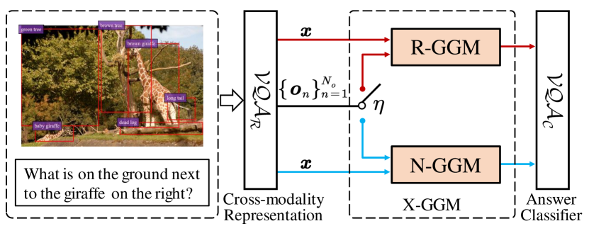
Figure 2. An overview of training a baseline VQA model using the X-GGM scheme. R-GGM and N-GGM are the two key modules of X-GGM. $\mathcal{{VQA_{R}}}$ and $\mathcal{{VQA_{C}}}$ indicate the Cross-modality Representation and Answer Classifier of a baseline VQA model, respectively.

Framework.

2. Related Work

2.1. OOD Generalization in VQA

Training and testing under the independent and identically distributed (i.i.d) setting have resulted in the performance of most VQA models being highly affected by superficial correlations (, language biases and dataset biases) (Zhang et al., 2016; Agrawal et al., 2016; Goyal et al., 2017; Agrawal et al., 2018). Recently, evaluation on the out-of-distribution (OOD) setting (Guo et al., 2019a; Teney et al., 2020c; Kervadec et al., 2020; Gokhale et al., 2020) has thus become an increasing concern for VQA. To improve the OOD generalization performance of VQA models, the prevailing methods target eliminating the language bias. Accordingly, current debiasing methods to VQA can be broadly divided into two groups, Known Bias-based (Clark et al., 2019; Chen et al., 2020b; Liang et al., 2020) and Unknown Bias-based (Teney et al., 2020b; Gokhale et al., 2020; Clark et al., 2020).

Known Bias-based methods consider the prior knowledge of language biases and design specific debiasing methods to reduce the biases explicitly existing in training set. Unknown Bias-based methods aim to remove the language bias or the answer distribution shift without the bias to be known in advance, which are more practical. In addition to considering extra human annotations (Selvaraju et al., 2019; Wu and Mooney, 2019; Gokhale et al., 2020) to balance datasets to reduce biases, most Unknown Bias-based methods leverage the adversarial training strategy (Grand and Belinkov, 2019; Teney et al., 2020a; Teney et al., 2020c; Gokhale et al., 2020; Li et al., 2020; Gan et al., 2020). Particularly, VILLA (Gan et al., 2020) introduces adversarial perturbations into embedding space and utilizes large-scale adversarial training to improve the generalization ability. Similarly, the proposed X-GGM scheme injects adversarial perturbations into representation space and utilizes the adversarial learning strategy based on graph generative modeling to achieve OOD generalization and to mitigate language biases without prior knowledge of these biases.

2.2. Graph Generative Models

Graph Generative Modeling (GGM), aiming to learn to generate new graphs with certain desirable properties by observing existing graphs, has emerged in biomedical (De Cao and Kipf, 2018), social science (Nauata et al., 2020), and graph representation learning (Yu et al., 2018; Pan et al., 2018; Wang et al., 2018). Recent advances in deep generative models, especially VAE (Kingma and Welling, 2013) and GAN (Goodfellow et al., 2014), have developed towards the graph domain, inspiring many graph generative models, such as GAE (Kipf and Welling, 2016b), GraphVAE (Simonovsky and Komodakis, 2018), GraphGAN (Wang et al., 2018), and Graphite (Grover et al., 2019). These graph generative models follow the uniform framework that includes generative and discriminative models, limiting the scale of generated graphs. In order to handle the challenge of scalability, deep autoregressive models are utilized for graph generation, such as GraphRNN (You et al., 2018), GRANs (Liao et al., 2019), and GraphAF (Shi et al., 2020). Furthermore, GRAM (Kawai et al., 2019) introduces graph attention mechanism to enable the graph generative model scalability.

Recent approaches consider improving the generalization ability of graph generative models. You  (You et al., 2020) propose GraphCL, a contrastive learning-based framework, to learn robust graph representations. Pan  (Pan et al., 2018) encode the topological structure and node content in a graph to obtain compact graph representations by a novel adversarial graph embedding framework. Dai  (Dai et al., 2018) propose ANE, an Adversarial Network Embedding framework, to leverage the adversarial learning principle to regularize the representation learning, contributing to the learning stable and robust graph representation. Zheng  (Zheng et al., 2020) propose DB-GAN, which implicitly bridges the graph and feature spaces by prototype learning, to learn more robust graph representation. The proposed X-GGM scheme considers generating both relationships between nodes and node representations during graph generative modeling to enhance the generalization ability of graph generative models.

2.3. Graph Construction in V+L Tasks

Graphs are non-Euclidean structured data, which can effectively represent relationships between nodes. Some recent works construct graphs for visual or linguistic elements in V+L tasks, such as VQA (Hu et al., 2019; Li et al., 2019b; Gao et al., 2020), VideoQA (Huang et al., 2020; Zhu et al., 2020b; Jiang and Han, 2020), Image Captioning (Yao et al., 2018; Guo et al., 2019b; Zhang et al., 2021), and Visual Grounding (Jing et al., 2020a; Liu et al., 2020; Yang et al., 2020b), to reveal relationships between these elements and obtain fine-grained semantic representations. These constructed graphs can be broadly grouped into three types: visual graphs between image objects/regions (, (Yao et al., 2018)), linguistic graphs between sentence elements/tokens (, (Kant et al., 2020)), and crossmodal graphs among visual and linguistic elements (, (Liu et al., 2020)). In this work, we construct the visual graph for X-GGM.

3. Preliminary

Taking the open-ended VQA task as a multi-class classification problem, the VQA model requires identifying the correct answer from a predefined set ($a\in\mathbb{A}$) of possible answers based on understanding the related question $q$ and image $I$. Commonly, a VQA model ($\mathcal{{VQA}}$) can be divided into two modules: Cross-modality Representation ($\mathcal{{VQA_{R}}}$) and Answer Classifier ($\mathcal{{VQA_{C}}}$), which can be formulated by

(1) $$\hat{a}=\mathcal{{VQA_{C}}}(a|{\bm{x}}),~{}{\bm{x}}=\mathcal{{VQA_{R}}}(q,I),$$

where, $\mathcal{{VQA_{R}}}$ is the crucial module of a VQA model, determining the representation ability of the VQA model. Therefore, the method aiming to achieve OOD generalization in VQA needs to improve the generalization performance while maintaining the representation ability of ${\bm{x}}$. In this paper, we consider two prevailing VQA models, , transformer-based model (LXMERT (Tan and Bansal, 2019)) and plain model (UpDn (Anderson et al., 2018)), as our baseline VQA models for evaluating the OOD performance of the proposed X-GGM scheme.

LXMERT. LXMERT (Tan and Bansal, 2019) is a classic transformer based on cross-modality pre-training, consisting of two single-modality encoders for visual and language modalities, respectively, and one cross-modality encoder for aligning entities across the two modalities. It can output a visual feature sequence $\{{\bm{o}}_{n}|{\bm{o}}_{n}\in\mathbb{R}^{d},1\leq n\leq N_{o}\}$, a language feature sequence, and the cross-modality feature vector ${\bm{x}}\in\mathbb{R}^{d}$, where, $N_{o}$ is the number of objects in one image, and $\bm{o}_{n}$ is the $n$-th object feature vector. The visual feature sequence $\{{\bm{o}}_{n}\}$ and the cross-modality feature vector ${\bm{x}}$ will be passed into the X-GGM scheme to improve the OOD generalization ability of ${\bm{x}}$ by generatively modeling new relationships between objects and new node representations.

UpDn. Bottom-Up Top-Down model (UpDn) (Anderson et al., 2018) is a typical attention based VQA model. For each image $I$, it utilizes an image encoder to output the sequence of object features: $\{{\bm{o}}_{n}|{\bm{o}}_{n}\in\mathbb{R}^{d},1\leq n\leq N_{o}\}$. For each question, it utilizes a question encoder to output the sequence of language features. After that, both the object and language features are fed into an attention module to obtain the joint representation ${\bm{x}}\in\mathbb{R}^{d}$ for answer prediction. $\{{\bm{o}}_{n}\}$ and ${\bm{x}}$ are the inputs of the X-GGM scheme.

Algorithm 1 Training a VQA Model with X-GGM

1:function X-GGM($I,q,a,{\bm{R}}_{GT}$)

2:     $\{{\bm{o}}_{n},1\leq n\leq N_{o}\},{\bm{x}}\leftarrow\mathcal{{VQA_{R}}}(I,q)$

3:     $cond\sim U[0,1]$

4:     if $cond\leq\eta$ then $\triangleright$ execute R-GGM

5:         ${\bm{R}}_{0}\leftarrow\textsc{Rinit}({\bm{x}},\sigma)$

6:         ${\bm{R}}_{g},\{\bar{{\bm{v}}}_{1},\dots,\bar{{\bm{v}}}_{N_{k}}\}\leftarrow\textsc{Rgen}(\{{\bm{o}}_{n}\},{\bm{R}}_{0})$

7:         $p_{a}\leftarrow\mathcal{{VQA_{C}}}({\bm{x}},\bar{{\bm{v}}}_{N_{k}})$

8:         $\mathcal{L}\leftarrow\textsc{Rlearn}({\bm{R}}_{g},{\bm{R}}_{GT},p_{a})$

9:     else$\triangleright$ execute N-GGM

10:         $\{{\bm{v}}_{i},1\leq i\leq N_{o}\}_{0}\leftarrow\textsc{Ninit}({\bm{x}},\sigma)$

11:         ${\bm{V}}_{g},\{\bar{{\bm{v}}}_{1},\dots,\bar{{\bm{v}}}_{N_{k}}\}\leftarrow\textsc{Ngen}(\{{\bm{v}}_{i}\}_{0},{\bm{R}}_{GT})$

12:         $p_{a}\leftarrow\mathcal{{VQA_{C}}}({\bm{x}},\bar{{\bm{v}}}_{N_{k}})$

13:         $\mathcal{L}\leftarrow\textsc{Nlearn}({\bm{V}}_{g},\{{\bm{o}}_{n}\},p_{a})$

14:     end if

15:end function

1:function $\mathrm{BMU}$($I,q,a$)

2:     $p_{a}\leftarrow\mathcal{{VQA}}(I,q,a)$ $\triangleright$ training baseline model

3:end function

4. Graph Generative Modeling

To improve the OOD generalization ability of ${\bm{x}}$ while preserving its representation ability, we consider the nature attribute of compositional generalization implicit in the information aggregation of graph nodes, and propose a Graph Generative Modeling-based training scheme (X-GGM). The overall process of training a baseline VQA model with the X-GGM scheme is shown in Algorithm 1, consisting of two parts: Graph Generative Modeling (X-GGM) and Baseline Model Update (BMU). Once $\mathcal{{VQA_{R}}}$ yields the cross-modality representation ${\bm{x}}$ and the sequence of visual feature vectors $\{{\bm{o}}_{n}|{\bm{o}}_{n}\in\mathbb{R}^{d},1\leq n\leq N_{o}\}$, X-GGM will update relationships between objects and representations of objects by Graph Relation Generative Modeling (R-GGM) and Graph Representation Generative Modeling (N-GGM) in each training update. In the following, we first introduce the predefined object-relation graph and then detail R-GGM and N-GGM.

4.1. Graph Construction

For the X-GGM scheme, we construct an object-relation graph using objects in one image as graph nodes. Specifically, the object-relation graph can be formulated as $\mathcal{G}=(\mathcal{V},{\bm{A}},{\bm{R}})$, where $\mathcal{V}=\{v_{1},\dots,v_{N_{o}}\}$ is a set of nodes with $|\mathcal{V}|=N_{o}$, ${\bm{A}}$ is the adjacency matrix with $a_{i,j}\in{\bm{A}}$ marking whether there is an edge between node $v_{i}$ and $v_{j}$, and ${\bm{R}}$ is a relation matrix describing the coherence between nodes. The constructed graph $\mathcal{G}$ is a fully-connected graph, meaning that the adjacency matrix ${\bm{A}}$ is an all-ones matrix. Therefore, we omit ${\bm{A}}$ in $\mathcal{G}$ for conciseness in following sections.

To determine the ground-truth (GT) of relation matrix ${\bm{R}}_{GT}$ utilizing in R-GGM, we compute the cosine similarity between object-class embeddings $\{{\bm{c}}_{n}|{\bm{c}}_{n}\in\mathbb{R}^{d},1\leq n\leq N_{o}\}$ and object-attribute embeddings $\{{\bm{a}}_{n}|{\bm{a}}_{n}\in\mathbb{R}^{d},1\leq n\leq N_{o}\}$. These embeddings (, ${\bm{c}}_{n}$ and ${\bm{a}}_{n}$) are obtained by a pre-trained BERT model (Devlin et al., 2018). Practically, the similarity computations are random combinations of object-classes and object-attributes in one image, which will breed new combinations. In N-GGM, the object feature ${\bm{o}}_{n}$ yielded by $\mathcal{{VQA_{R}}}$ serves as the GT of the $i$-th node representation (, ${\bm{v}}_{GT,i}={\bm{o}}_{n}$).

4.2. Graph Relation Generative Modeling

Graph Relation Generative Modeling (R-GGM) consists of three stages: initializing relation matrix utilizing ${\bm{x}}$ and Gaussian noise (Rinit), Graph Relation Matrix Generation (Rgen), and Adversarial Learning of Relation (Rlearn).

Initializing Relation Matrix (Rinit). The graph $\mathcal{G}$ is an undirected graph with $N_{o}$ nodes. Therefore, the relation matrix ${\bm{R}}\in\mathbb{R}^{N_{o}\times N_{o}}$ is symmetric, meaning that only the upper triangular elements without diagonal elements (always 1) need to be initialized. Specifically, we first transform ${\bm{x}}$ into a vector ${\bm{r}}\in\mathbb{R}^{N_{o}(N_{o}-1)/2}$ by

(2) $${\bm{r}} =\mathit{Sigmoid}\left({\bm{W}}_{r}{\bm{x}}+{\bm{b}}_{r}\right),$$

where, ${\bm{W}}_{r}\in\mathbb{R}^{N_{o}(N_{o}-1)/2\times d}$ is the transformation matrix, the learnable bias ${\bm{b}}_{r}$ has same size as ${\bm{r}}$, and $\mathit{Sigmoid}$ denotes the Sigmoid activation function. Subsequently, we inject the adversarial perturbation (, Gaussian noise) to ${\bm{r}}$ and make $\hat{{\bm{r}}}\sim p_{\sigma}(\hat{{\bm{r}}}|{\bm{r}})$:

(3) $$p_{\sigma}(\hat{{\bm{r}}}|{\bm{r}})=\frac{1}{\sqrt{2\pi}\sigma}\exp\{-\frac{(\hat{{\bm{r}}}-{\bm{r}})^{2}}{2\sigma^{2}}\},$$

where $\sigma$ is the standard deviation of Gaussian noise. Finally, we sequentially fill the upper triangular part (${\bm{R}}_{0}^{\bot}$) of ${\bm{R}}_{0}$ with the elements of $\hat{{\bm{r}}}$, and obtain the initial relation matrix by ${\bm{R}}_{0}={\bm{R}}_{0}^{\bot}+({\bm{R}}_{0}^{\bot})^{\mathrm{T}}$.

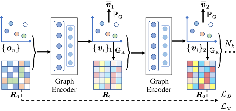
Figure 3. Graph Relation Generation. $\mathbb{P}_{\text{G}}$ indicates the average pooling of node representations, and $\mathbb{G}_{\text{R}}$ denotes generating relation matrix by Eq. (6).

Architecture of Rgen.

Relation Matrix Generation (Rgen). The detailed process of Rgen is shown in Figure. 3, which can be accomplished in $N_{k}$ iterations. Before the iteration beginning, node representations of the graph $\mathcal{G}$ are initialized by the corresponding object feature vector, , ${\bm{v}}_{i}={\bm{o}}_{n}$ ($i=n$). In the $k$-th ($1\leq k\leq N_{k}$) iteration, node representations ${\bm{V}}_{k-1}=\{{\bm{v}}_{i}\}_{k-1}$ and the relation matrix ${\bm{R}}_{k-1}$ yielded by Graph Encoder in the $(k-1)$-th iteration are first fed into the $k$-th Graph Encoder and served as inputs (, ${\bm{V}}_{k}^{(0)}={\bm{V}}_{k-1}\in\mathbb{R}^{N_{o}\times d}$ and ${\bm{R}}_{k}^{(0)}={\bm{R}}_{k-1}\in\mathbb{R}^{N_{o}\times N_{o}}$). Subsequently, the node representations are encoded by Graph Encoder, which is essentially a GCN (Kipf and Welling, 2016a) with $N_{l}$-layers. Specifically, the node representations in the $l$-layer of Graph Encoder can be updated with

(4) $${\bm{V}}^{(l+1)}_{k}=\mathit{Sigmoid}(({\bm{R}}_{k}^{(0)}{\bm{V}}^{(l)}_{k}){\bm{W}}^{(l)}_{k}+{\bm{b}}^{(l)}_{k}),$$

where, ${\bm{W}}^{l}_{k}\in\mathbb{R}^{N_{o}\times d\times d}$ is spanned by $N_{o}$ matrices of feature transformation, and ${\bm{b}}_{k}^{l}\in\mathbb{R}^{N_{o}\times d}$ is the learnable bias for the transformation. After that, we assemble the input and the output of each layer in Graph Encoder to obtain the final output ${\bm{V}}_{k}$ of the $k$-th iteration:

(5) $${\bm{V}}_{k}=\sum_{l=0}^{N_{l}}\mathit{ReLU}({\bm{V}}_{k}^{(l)}{\bm{W}}_{a}+{\bm{b}}_{a}),$$

where, $\mathit{ReLU}$ denotes the ReLU activation function, ${\bm{W}}_{a}\in\mathbb{R}^{N_{o}\times d\times d}$ and ${\bm{b}}_{a}\in\mathbb{R}^{N_{o}\times d}$ are the weight and bias for node feature transformation, respectively. Finally, the relation matrix is generated using the final node representations ${\bm{V}}_{k}$ by

(6) $${\bm{R}}_{k}=\mathit{Sigmoid}({\bm{V}}_{k}{\bm{V}}_{k}^{\mathrm{T}}).$$

We utilize the output of the last iteration as the final generated relation matrix, that is, ${\bm{R}}_{g}={\bm{R}}_{N_{k}}$. In addition, we average node representations $\{{\bm{v}}_{i},1\leq i\leq N_{o}\}_{k}$ to derive the graph representation $\bar{{\bm{v}}}_{k}$ in the $k$-th iteration.

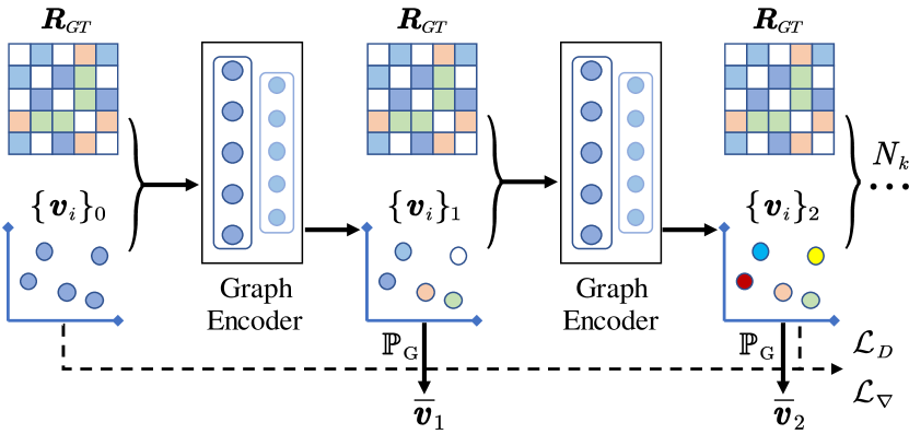
Figure 4. Graph Representation Generation. $\mathbb{P}_{\text{G}}$ is an average operation of node representations.

Architecture of Ngen.

Adversarial Learning of R-GGM (Rlearn). When initializing the relation matrix in the stage of Rinit, we find that the process of R-GGM introducing adversarial perturbations is similar to that of Denoising AutoEncoder (Vincent et al., 2008). From the works (Li et al., 2019a; Bigdeli et al., 2020), we know that the optimal Denoising AutoEncoder for additive white Gaussian noise (AWGN) can be explicitly calculated, which is related to the gradient of the data distribution after adding noises. Practically, the logarithmic gradient of the data distribution with adversarial perturbations can be deduced from Eq. (3):

(7) $$\nabla_{\hat{{\bm{r}}}}\log p_{\sigma}(\hat{{\bm{r}}}|{\bm{r}})=-\frac{(\hat{{\bm{r}}}-{\bm{r}})^{2}}{\sigma^{2}}.$$

After obtaining $\nabla_{\hat{{\bm{r}}}}\log p_{\sigma}(\hat{{\bm{r}}}|{\bm{r}})$, we can compute the gradient of log-likelihood estimation, , $\nabla_{{\bm{r}}}\log p_{g}({\bm{r}})$, of elements in the generated relation matrix ${\bm{R}}_{g}$ to constrain the gradient distribution consistency between the generated relation matrix ${\bm{R}}_{g}$ and the pre-derived similarity matrix ${\bm{R}}_{GT}$. Therefore, the gradient distribution consistency loss can be defined as

(8) $$\mathcal{L}_{\nabla}\triangleq\mathbb{E}\left[\left\|\nabla_{{\bm{r}}}\log p_{g}({\bm{r}})-\nabla_{\hat{{\bm{r}}}}\log p_{\sigma}(\hat{{\bm{r}}}|{\bm{r}})\right\|_{2}^{2}\right].$$

In addition to constraining the gradient distribution consistency, we further utilize KL-Divergence to measure the distance between the generated distribution $p_{g}({\bm{r}})$ and the raw data distribution $p_{data}({\bm{r}})$, where $p_{g}$ and $p_{data}$ denote probability distributions of elements in matrix ${\bm{R}}_{g}$ and ${\bm{R}}_{GT}$, respectively. The distance measure loss of training our R-GGM can be formulated by

(9) $$\mathcal{L}_{D}=\mathrm{KL}(p_{g}\|p_{data})+\mathrm{KL}(p_{data}\|p_{g}),$$

where, $\mathrm{KL}(p\|q)=\mathbb{E}_{{\bm{r}}\sim p}\left[\log p({\bm{r}})-\log q({\bm{r}})\right]$.

Besides the adversarial losses (, $\mathcal{L}_{\nabla}$ and $\mathcal{L}_{D}$), we compute the BCE loss ($\mathcal{L}_{\textsc{bec}}$) of the VQA task by adding ${\bm{x}}$ (the original cross-modality representation) and $\bar{{\bm{v}}}_{N_{k}}$ (the graph representation yielded by the last iteration in Rgen) and passing the value into $\mathcal{{VQA_{C}}}$ to derive the likelihood estimation of answer distribution $p_{a}$.

In summary, the total loss of training R-GGM can be formulated by

(10) $$\mathcal{L}=\alpha\mathcal{L}_{\nabla}+\beta\mathcal{L}_{D}+\mathcal{L}_{\textsc{bce}},$$

where, $\alpha$ and $\beta$ are weighted coefficients.

Table 1. Statistics of VQA-CP v2 and GQA-OOD.

Dataset	Image					Question					Year
	Train	Val	OOD Test	ID Test	Total	Train	Val	OOD Test	ID Test	Total
VQA-CP v2 (Agrawal et al., 2018)	[log][r]119,107	[log][r]31,976	[log][r]89,437	[log][r]32,266	[log][r]272,786	[log][r]388,735	[log][r]38,802	[log][r]179,928	[log][r]40,000	[log][r]647,465	2018
GQA-OOD (Kervadec et al., 2020)	[log][r]72,140	[log][r]9,406	[log][r]330	[log][r]365	[log][r]82,241	[log][r]943,000	[log][r]51,045	[log][r]1,063	[log][r]1,733	[log][r]996,841	2020

4.3. Graph Representation Generative Modeling

Graph Representation Generative Modeling (N-GGM) is similar to R-GGM, which can also be implemented in three stages: initializing node representations with ${\bm{x}}$ and Gaussian noise (Ninit), Graph Node Representation Generation (Ngen), and Adversarial Learning of Node Representation (Nlearn).

Initializing Node Representations (Ninit). To obtain the $N_{o}$ initial node representations of the graph $\mathcal{G}$, we first span ${\bm{x}}$ to $[{\bm{x}},\dots,{\bm{x}}]\in\mathbb{R}^{N_{o}\times d}$, and utilize a fully-connected layer ($\mathcal{M}_{\text{FC}}$) to increase the variability of node representations:

(11) $${\bm{V}}_{{\bm{x}}} =\mathcal{M}_{\text{FC}}([{\bm{x}},\dots,{\bm{x}}]),{\bm{V}}_{{\bm{x}}}\in\mathbb{R}^{N_{o}\times d},$$

where, ${\bm{V}}_{{\bm{x}}}=\{{\bm{v}}_{i,{\bm{x}}}|{\bm{v}}_{i,{\bm{x}}}\in\mathbb{R}^{d}\},1\leq i\leq N_{o}$. After that, we inject adversarial perturbations to ${\bm{V}}_{{\bm{x}}}$, and make the sampled feature vector $\hat{{\bm{v}}}_{i,{\bm{x}}}$ of the $i$-th element in ${\bm{V}}_{{\bm{x}}}$ satisfy the noise prior distribution $p_{\sigma}(\hat{{\bm{v}}}_{i,{\bm{x}}}|{\bm{v}}_{i,{\bm{x}}})$:

(12) $$p_{\sigma}(\hat{{\bm{v}}}_{i,{\bm{x}}}|{\bm{v}}_{i,{\bm{x}}})=\frac{1}{\sqrt{2\pi}\sigma}\exp\{-\frac{(\hat{{\bm{v}}}_{i,{\bm{x}}}-{\bm{v}}_{i,{\bm{x}}})^{2}}{2\sigma^{2}}\}.$$

Finally, the initial node representations of the graph $\mathcal{G}$ can be obtained by ${\bm{V}}_{0}=\hat{{\bm{V}}}_{{\bm{x}}}=[\hat{{\bm{v}}}_{0,{\bm{x}}},\dots,\hat{{\bm{v}}}_{N_{o},{\bm{x}}}]$.

Node Representation Generation (Ngen). The details of Ngen are shown in Figure 4. In the $k$-th iteration, the node representations ${\bm{V}}_{k-1}=\{{\bm{v}}_{i},1\leq i\leq N_{o}\}_{k-1}$ generated by Graph Encoder in the $(k-1)$-th iteration and the predefined GT relation matrix ${\bm{R}}_{GT}$ are first passed into the $k$-th Graph Encoder to update the node representations of each layer. After that, the final output of the $k$-th Graph Encoder ${\bm{V}}_{k}$ can be obtained by Eq. (5). The architecture of Graph Encoder in N-GGM is the same as that in R-GGM. We utilize the output of the last iteration as the generated node representations, , ${\bm{V}}_{g}={\bm{V}}_{N_{k}}$. Besides, in each iteration, we average $N_{o}$ node representations and yield the graph representation $\bar{{\bm{v}}}_{k}$.

Adversarial Learning of N-GGM (Nlearn). The total loss $\mathcal{L}$ of training N-GGM is also a weighted sum of $\mathcal{L}_{\nabla}$, $\mathcal{L}_{D}$, and $\mathcal{L}_{\textsc{bce}}$. Specifically, the gradient distribution consistency loss $\mathcal{L}_{\nabla}$ is defined as the distance between the distribution gradient of the initial node representations after adding Gaussian noise ($\hat{{\bm{V}}}_{{\bm{x}}}$) and the log-likelihood estimation of generated node representations (${\bm{V}}_{g}$). $\mathcal{L}_{D}$ is the KL-Divergence loss between the distribution of generated node representations (${\bm{V}}_{g}$) and the distribution of the raw node representations ($\{{\bm{o}}_{n}\}$) yielded by $\mathcal{{VQA_{R}}}$. The VQA classification loss $\mathcal{L}_{\textsc{bce}}$ is the same as the corresponding term in Eq. (10).

5. Experiments

In this section, we evaluate the effectiveness of X-GGM key components and compare the proposed X-GGM scheme with state-of-the-art approaches on two standard VQA OOD benchmarks, , VQA-CP v2 (Agrawal et al., 2018) and GQA-OOD (Kervadec et al., 2020). Table 1 reports the statistics of experimental datasets.

5.1. Experimental Settings

Table 2. Ablation studies on R-GGM and N-GGM with different combinations of $\mathcal{L}_{D}$ and $\mathcal{L}_{\nabla}$ (More results are shown in Table 6 of the Appendix). $\uparrow$ ($\downarrow$) indicates the higher (lower) the better. LX. means the Baseline, , LXMERT.

S/N	R-GGM		N-GGM		VQA-CP v2			GQA-OOD
	$\mathcal{L}_{\nabla}$	$\mathcal{L}_{D}$	$\mathcal{L}_{\nabla}$	$\mathcal{L}_{D}$	OOD$\uparrow$	ID$\uparrow$	Gap$\downarrow$	Tail$\uparrow$	Head$\uparrow$	$\Delta$$\downarrow$
LX.	—				59.98	65.21	5.23	49.80	57.70	15.90
#1	✓	✓			63.84	66.41	2.57	51.39	56.93	10.77
#2			✓	✓	62.90	65.57	2.67	51.27	57.30	11.76
#3	✓		✓		63.75	66.03	2.28	51.65	57.13	10.61
#4		✓		✓	62.73	65.99	3.26	51.27	57.19	11.54
#5	✓	✓	✓	✓	64.33	66.92	2.59	52.47	57.51	9.59

5.1.1. Evaluation Benchmarks

VQA-CP v2. It is the reorganization of the training and validation sets of VQA v2.0 (Shih et al., 2016). To evaluate the OOD generalization performance of existing VQA models, Agrawal  (Agrawal et al., 2018) construct VQA-CP v2 by ensuring that the answer distribution of per question type in the test set and the training set is different. The original VQA-CP v2 only consists of the test set (about 98K images, 220K questions, and 2.2M answers) and the training set (about 121K images, 438K questions, and 4.4M answers). That is, the benchmark does not have an official validation set.

GQA-OOD. It is a fine-grained restructuring of GQA (Hudson and Manning, 2019), which obtains the validation and test sets by introducing answer distribution shifts into the validation and test sets of GQA. However, GQA-OOD shares the same training set with GQA. The GQA-OOD benchmark provides four metrics. 1) Tail: accuracy on OOD samples (, samples of the tail of the answer class distribution), 2) Head: accuracy on in-domain (ID) samples (, samples from the head distribution, 3) All: overall accuracy on all test samples, and 4) $\Delta(\%)\textup{ = (head - tail) / tail}$: a new evaluation protocol proposed by Kervadec  (Kervadec et al., 2020) to illustrate how much is the error prediction imbalanced between frequent and rare answers.

5.1.2. Experimental Details

Data Preprocessing. As Teney  (Teney et al., 2020c) discussed, there are several pitfalls in evaluating VQA models under the OOD setting on VQA-CP v2, especially using the OOD test set for model selection and evaluating the ID performance of a VQA model after retraining the model on VQA v2.0 (Shih et al., 2016). Therefore, following recent works (Teney and Hengel, 2019; Teney et al., 2020b, a; Clark et al., 2020), we re-split VQA-CP v2. Specifically, we reserve 40k random samples from the train set to evaluate the in-domain (ID) performance and 40k random instances from the test set for model selection. Besides, the bottom-up attention Faster R-CNN (Anderson et al., 2018) pre-trained on Visual Genome (Krishna et al., 2017) is utilized to obtain object class and attribute in the image for the two datasets.

Implementation Details. For X-GGM, we set the number $N_{o}$ of nodes in $\mathcal{G}$ to 36 and the standard feature dimensionality $d$ to 768. The standard deviation $\sigma$ in Eq. (3) is 1.0. The threshold $\eta$ in Algorithm 1 are 0.8 and 0.5 for VQA-CP v2 and GQA-OOD, respectively. The total step $N_{k}$ of X-GGM is 2, and the layer $N_{l}$ of the encoder in each step is 2. The weight coefficients $\alpha$ and $\beta$ in Eq. (10) are 6 and 72 for R-GGM, and 6.6 and 0.17 for N-GGM. All experiments are implemented on one NVIDIA GTX2080 12GB GPU for 5 epochs with a batch size of 128 and a learning rate of 1e-6.

5.2. Ablation Studies

We conduct ablation studies on key components of X-GGM using LXMERT as the baseline VQA model. Considering the discovery in work (Teney et al., 2020c), , the questions with yes/no/number answers on VQA-CP v2 are easier to game, for a fairer comparison, we train all models on VQA-CP v2 “All”. But, we select the best model and focus the model analysis on VQA-CP v2 “other”.

5.2.1. Effectiveness of Key Components

R-GGM / N-GGM / X-GGM vs. Baseline. To improve the OOD generalization ability of the cross-modality representation ${\bm{x}}$ yielded by $\mathcal{{VQA_{R}}}$, besides training the baseline VQA model using the full X-GGM scheme, R-GGM and N-GGM can also work independently. Therefore, we consider comparisons between the ablated components (#1, #2, #5) and the Baseline, , LXMERT (LX.) in Table 2 to evaluate the respective effects of R-GGM, N-GGM, and X-GGM. Specifically, $\blacktriangleright$ LX. #1 (only using R-GGM in the training process). $\blacktriangleright$ LX. #2 (only using N-GGM in the training process). $\blacktriangleright$ LX. #5 (using the full X-GGM scheme that executes R-GGM and N-GGM at a ratio of $\eta$ in the training process). Table 2 shows the results on VQA-CP v2 “Other” and GQA-OOD. LX. #5 demonstrates the effectiveness of X-GGM. LX. #1 / #2 illustrates that the single R-GGM / N-GGM can also effectively improve the OOD generalization performance of the baseline VQA model.

R-GGM / N-GGM vs. X-GGM. In each training iteration, X-GGM randomly executes R-GGM or N-GGM to improve the OOD generalization ability of the baseline VQA model. To explore the importance of R-GGM and N-GGM to the full training scheme (X-GGM), as shown in Table 2 (#1, #2, #5), we conduct the following comparisons: $\blacktriangleright$ #1 #5, and $\blacktriangleright$ #2 #5. The results in Table 2 indicate that R-GGM is more effective than N-GGM for the X-GGM scheme in boosting the OOD performance of the baseline VQA model (LXMERT) on both VQA-CP v2 “Other” and GQA-OOD. This is mainly because the gradient instability caused by the noise introduction in N-GGM is larger than that in R-GGM. Specifically, the noise vector dimensions introduced into R-GGM and N-GGM are $N_{o}(N_{o}-1)/2=630$ and $N_{o}\times d=27,648$, respectively.

Gradient Distribution Consistency Loss. To evaluate the effectiveness of the gradient distribution consistency loss $\mathcal{L}_{\nabla}$ in alleviating the unstable gradient issue, we compare the respective effects of $\mathcal{L}_{\nabla}$ and $\mathcal{L}_{D}$. The KL-Divergence loss $\mathcal{L}_{D}$ is also an adversarial loss. The experimental settings are shown in Table 2 (#3, #4, #5). More specifically, $\vartriangleright$ #$\mathsf{3}$: only using $\mathcal{L}_{D}$ as the adversarial loss to train the baseline VQA model (LXMERT) with the X-GGM scheme, $\vartriangleright$ #$\mathsf{4}$: only using $\mathcal{L}_{\nabla}$ as the adversarial loss to train the baseline VQA model with the X-GGM scheme, and $\vartriangleright$ #$\mathsf{5}$: using a weighted sum of $\mathcal{L}_{\nabla}$ and $\mathcal{L}_{D}$ as the adversarial loss to train the baseline VQA model with the X-GGM scheme. The comparisons between #3, #4, and #5 on VQA-CP v2 “Other” and GQA-OOD in Table 2 illustrate that both $\mathcal{L}_{D}$ and $\mathcal{L}_{\nabla}$ are effective for training the baseline VQA model with the X-GGM scheme. However, $\mathcal{L}_{\nabla}$ performs better than $\mathcal{L}_{D}$, demonstrating the effectiveness of $\mathcal{L}_{\nabla}$ in alleviating unstable gradient updates in graph adversarial learning.

Table 3. Comparisons between different variants of Graph Encoder (GEnc.) with $N_{l}$ layers.

GEnc.	$N_{l}$	VQA-CP v2			GQA-OOD
		OOD$\uparrow$	ID$\uparrow$	Gap$\downarrow$	Tail$\uparrow$	Head$\uparrow$	$\Delta$$\downarrow$
LX.	—	59.98	65.21	5.23	49.80	57.70	15.90
GCN	1	64.10	66.70	2.60	51.65	57.24	10.83
	2	64.33	66.92	2.59	52.47	57.51	9.59
GIN	1	63.62	66.24	2.62	50.99	57.08	11.93
	2	63.83	66.39	2.56	51.27	57.30	11.76
GAT	1	63.94	66.40	2.46	51.65	57.71	11.73
	2	63.94	66.45	2.51	50.99	56.90	11.59

Table 4. Comparisons with UB-based debiasing methods on VQA-CP v2 (full comparisons with state-of-the-arts are reported in Table 7 of the Appendix). ^†: methods using additional manually annotated data, ^∗: results from our reimplementation using the official released code, —: not reported.

Method	VQA-CP v2 (OOD Test) $\uparrow$				VQA-CP v2 (ID Test) $\uparrow$				Gap $\downarrow$
	All	Yes/No	Num.	Other	All	Yes/No	Num.	Other	All	Yes/No	Num.	Other
Unshuffling (Teney et al., 2020b)	42.39	47.72	14.43	47.24	—	—	—	—	—	—	—	—
Unshuffling+CF (Teney et al., 2020a)	40.60	61.30	15.60	46.00	63.30	79.40	45.50	53.70	22.70	18.10	29.90	7.70
Unshuffling+CF+GS (Teney et al., 2020a)	46.80	64.50	15.30	45.90	62.40	77.80	43.80	53.60	15.60	13.30	28.50	7.70
UpDn (Anderson et al., 2018)	38.82	42.98	12.18	43.95	64.73	79.45	49.59	55.66	25.91	36.47	37.32	11.71
+ Top answer masked (Teney et al., 2020c)	40.61	82.44	27.63	22.26	30.90	44.12	5.00	20.85	9.71	38.32	22.63	1.41
+ AdvReg (Grand and Belinkov, 2019)	36.33	59.33	14.01	30.41	50.63	67.39	38.81	38.37	14.30	8.06	24.80	7.96
+ GRL (Grand and Belinkov, 2019)	42.33	59.74	14.78	40.76	56.90	69.23	42.50	49.36	14.57	9.49	27.72	8.60
+ RandImg ($\lambda$=12) (Teney et al., 2020c)	55.37	83.89	41.60	44.20	54.24	64.22	34.40	50.46	1.13	19.67	7.20	6.26
+ RandImg ($\lambda$=5) (Teney et al., 2020c)	51.15	75.06	24.30	45.99	59.28	70.66	43.06	53.40	8.13	4.40	18.76	7.41
+ MUTANT† (Gokhale et al., 2020)	61.72	88.90	49.68	50.78	—	—	—	—	—	—	—	—
+ X-GGM	45.71	43.48	27.65	52.34	67.16	83.74	48.26	56.91	21.45	40.26	20.61	4.57
LXMERT∗ (Tan and Bansal, 2019)	63.90	80.45	46.58	59.98	75.57	91.39	59.83	65.21	11.67	10.94	13.25	5.23
+ MUTANT† (Gokhale et al., 2020)	69.52	93.15	67.17	57.78	—	—	—	—	—	—	—	—
+ VILLA∗ (Gan et al., 2020)	48.06	42.66	18.97	58.89	75.85	90.40	60.02	66.66	27.79	47.74	41.05	7.77
+ X-GGM	66.95	78.91	53.63	64.33	75.88	90.18	60.06	66.92	8.93	11.27	6.43	2.59

5.2.2. Variants of Graph Encoder

In the proposed X-GGM scheme, Graph Encoder is a general block utilized to aggregate node information and encode relationships between nodes. That is, architecture differences between different Graph Encoders can not markedly affect the performance of X-GGM to OOD generalization. To demonstrate that the X-GGM scheme is robust for different variants of Graph Encoder, we consider three prevailing Graph Neural Networks (, GCN (Kipf and Welling, 2016a), GIN (Xu et al., 2018), and GAT (Veličković et al., 2017)) and set the number of their layers $N_{l}$ to 1 and 2. From the results on VQA-CP v2 “Other” and GQA-OOD shown in Table 3, we can observe that there is only a slight difference between the OOD performance of different Graph Encoder variants. However, all of these variants have achieved dramatic improvements in OOD performance compared with the baseline VQA model (LXMERT). The results demonstrate that X-GGM is agnostic to Graph Encoder and is robust for different Graph Encoders.

5.2.3. Hyperparameter

Ratio of R-GGM and N-GGM $\eta$. The threshold $\eta$ in Algorithm 1 determines the ratio of R-GGM and N-GGM executed in each training iteration. To analyze the influence of $\eta$ for X-GGM improving the OOD performance, we conduct some ablated experiments on different values of $\eta$, , $\eta\in\{0.1,0.2,\dots,0.9\}$. Results on VQA-CP v2 “Other” and GQA-OOD are shown in Figure 5 (a) and (b), respectively. We observe that the baseline VQA model (LXMERT) trained with the proposed X-GGM scheme can achieve the best OOD performance on VQA-CP v2 “Other” and GQA-OOD when $\eta$ = 0.8 and $\eta$ = 0.5, respectively. The average gains of the OOD performance on VQA-CP v2 “Other” and GQA-OOD are $+3.76_{\pm 0.36}$ and $+1.54_{\pm 0.59}$, respectively. Comparing the OOD performance gains (the baseline VQA model) with the standard deviations of the OOD performance, we can consider the performance fluctuation is slight, demonstrating the robustness of the X-GGM scheme to the hyperparameter $\eta$.

5.3. Comparisons with State-of-the-Arts

To evaluate the OOD and ID performance of baseline VQA models trained with the proposed X-GGM scheme, we compare them with state-of-the-art methods on VQA-CP v2 and GQA-OOD.

5.3.1. Performance on VQA-CP v2

Setting. X-GGM is a training scheme for improving the OOD generalization ability of baseline VQA models while preserving the ID performance, which alleviates the language bias in VQA to some extent without the bias being known in advance. Therefore, according to whether debiasing methods need to know the bias existing on the datasets beforehand, we group them into two types. (1) Known Bias-based (KB-based) methods, such as LMH (Clark et al., 2019), LRS (Guo et al., 2020), and LMH-MFE (Gat et al., 2020). (2) Unknown Bias-based (UB-based) methods, such as MCE (Clark et al., 2020), MUTANT (Gokhale et al., 2020), Unshuffling (Teney et al., 2020b), and VILLA (Gan et al., 2020). Particularly, VILLA (Gan et al., 2020) utilizes the adversarial training strategy that introduces noises into representation space to improve model generalization ability. The strategy of injecting adversarial perturbations into representation space inspired our work. Therefore, we reimplement VILLA (Gan et al., 2020) on VQA-CP v2 for a fairer comparison. On VQA-CP v2, we utilize LXMERT and UpDn as baseline VQA models and mainly compare the proposed X-GGM scheme with UB-based methods (more comparisons with state-of-the-art methods are shown in the Appendix). As with ablation study, we implement our experiments on VQA-CP v2 “All” but focus comparisons on “Other”, which can better evaluate the ability of approaches to OOD generalization than “Yes/No” and “Num.”.

Results. Comparisons are reported in Table 4. As shown in the table, facilitated by the proposed X-GGM scheme, the baseline VQA model (LXMERT) achieves state-of-the-art OOD and ID performance on VQA-CP v2 “Other”. Besides, compared with all methods utilized UpDn as the baseline VQA model, our method also gains the best OOD and ID performance on “Other”. These results demonstrate the X-GGM scheme is effective for a VQA model to generalize to out-of-distribution samples while preserving its ID performance.

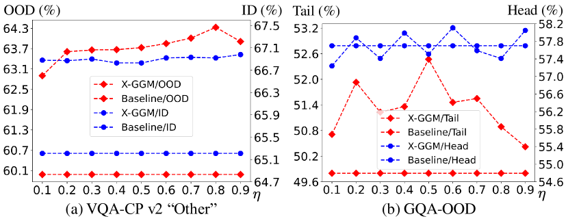
Figure 5. Ablation studies on the hyperparameter $\eta$. (a) OOD and ID accuracies of our method (X-GGM) and the Baseline (LXMERT) on VQA-CP v2 “Other”. (b) OOD (Tail) and ID (Head) accuracies on GQA-OOD.

Hyparameter.

5.3.2. Performance on GQA-OOD

Table 5. Comparisons with state-of-the-arts on GQA-OOD.

Method	Metrics (%)
	All $\uparrow$	Tail $\uparrow$	Head $\uparrow$	$\Delta$ $\downarrow$
Plain Models
BAN4 (Kim et al., 2018)	50.20	47.20	51.90	9.90
MMN (Chen et al., 2021)	52.70	48.00	55.50	15.60
UpDn (Anderson et al., 2018)	46.40	42.10	49.10	16.60
+ LMH (Clark et al., 2019)	33.10	30.80	34.50	12.00
+ LM (Clark et al., 2019)	34.50	32.20	35.90	11.50
+ RUBi (Cadene et al., 2019)	38.80	35.70	40.80	14.30
+ X-GGM	48.41	45.99	49.90	8.51
Transformer-based Models
MCAN (Yu et al., 2019)	50.80	46.50	53.40	14.80
MANGO (Li et al., 2020)	56.40	51.27	59.55	16.15
LXMERT (Tan and Bansal, 2019)	54.60	49.80	57.70	15.90
+ VILLA∗ (Gan et al., 2020)	54.47	49.95	57.24	14.59
+ MANGO (Li et al., 2020)	54.94	—	—	—
+ X-GGM	55.59	52.47	57.51	9.59

Settings. Except for LMH (Clark et al., 2019) and LM (Clark et al., 2019), the other methods listed in Table 5 are UB-based and can be further grouped into plain models (models in the third row of Table 5, , BAN4 (Kim et al., 2018) and MMN (Chen et al., 2021)) and transformer-based models (models in the fourth row of Table 5 like MCAN (Yu et al., 2019) and VILLA (Gan et al., 2020)). We utilize LXMERT and UpDn as baseline VQA models, and compare the proposed X-GGM scheme with all existing methods on GQA-OOD. Specifically, RUBi (Cadene et al., 2019), LMH (Clark et al., 2019) and LM (Clark et al., 2019) utilize UpDn as their baseline model. VILLA (Gan et al., 2020) and MANGO (Li et al., 2020) use LXMERT as the baseline VQA model. We also reimplement VILLA on GQA-OOD.

Results. From the comparisons in Table 5, we can observe that benefiting from the OOD generalization ability of X-GGM, the baseline VQA model (LXMERT) trained with our scheme outperforms all other methods on GQA-OOD on the metric Tail. Although the ID performance (Head) drops by 0.19 relative to the baseline VQA model, it is far smaller than the OOD performance improvement (2.67). Besides, the baseline VQA model (UpDn) trained with the X-GGM scheme also outperforms these methods utilized UpDn as the baseline VQA model on all metrics, especially on Tail. These results demonstrate the ability of the proposed X-GGM scheme to OOD generalization and ID preserving. Unfortunately, the OOD performance improvement on GQA-OOD is not as obvious as that on VQA-CP v2. It likely because questions of GQA-OOD are semantic compositionality. The syntax-complex questions weaken the representation ability of ${\bm{x}}$ while X-GGM also does not explicitly leverage the structured representation of question to enhance ${\bm{x}}$.

5.4. Qualitative Examples

To qualitatively illustrate the effectiveness of the X-GGM scheme in improving the OOD performance of baseline VQA models, we show some prediction examples from the OOD test sets of VQA-CP v2 and GQA-OOD. As shown in Figure 6, the Baseline (, LXMERT) is prone to utilize in-domain answers (, eating and sitting) to answer out-of-distribution questions. In contrast, the Baseline after being trained with the proposed X-GGM scheme can yield out-of-distribution answers, such as brushing teeth and posing in the first row of Figure 6, demonstrating the ability of X-GGM to OOD generalization. More predictions and visualization of the generated relation matrices are shown in Figure 7-8 of the Appendix.

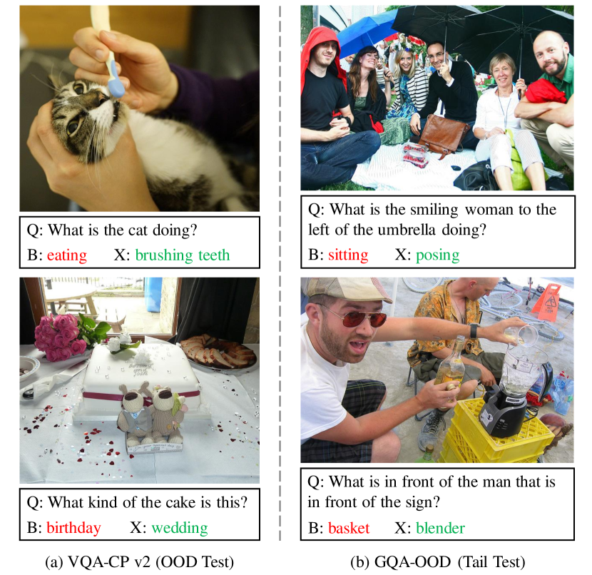
Figure 6. Qualitative examples from the OOD test set of VQA-CP v2 and GQA-OOD respectively provided by the Baseline (B), , LXMERT, and the Baseline trained with the X-GGM scheme (X). The wrong and correct answers are highlighted in red and green, respectively.

Vis.

6. Conclusion

In this paper, we proposed a Graph Generative Modeling-based scheme, X-GGM, to improve the OOD generalization ability of baseline VQA models while preserving the ID performance. Specifically, the X-GGM scheme randomly executes R-GGM or N-GGM to generate a new relation matrix or new node representations to enable the baseline VQA model to generalize to out-of-distribution samples. Besides, to alleviate the unstable gradient issue in graph adversarial learning, we propose a gradient distribution consistency loss to constrain the derivative of data distribution with adversarial perturbations and generated distribution. We evaluate the effectiveness of X-GGM components by extensive and ablative experiments. The baseline VQA model (LXMERT) trained with the proposed X-GGM scheme achieves state-of-the-art OOD performance on two VQA OOD benchmarks while preserving the ID performance.

Appendix A Appendix

A.1. More Experimental Results

Ablation Studies. The results in Table 2 indicate that a single R-GGM or N-GGM can also effectively improve the OOD generalization ability of baseline VQA models in addition to the full X-GGM scheme, and $\mathcal{L}_{\nabla}$ is more effective than $\mathcal{L}_{D}$ for alleviating the unstable gradient issue when training the baseline VQA model with the X-GGM scheme. To further illustrate the effectiveness of $\mathcal{L}_{\nabla}$ when training the Baseline with single R-GGM or N-GGM, as shown in Table 6 (#6, #7, #8, #9), we conduct more ablated experiments. Specifically, $\vartriangleright$ #6 only using $\mathcal{L}_{\nabla}$ as the adversarial loss to train the baseline VQA model (LXMERT) with the R-GGM. $\vartriangleright$ #7 only using $\mathcal{L}_{D}$ as the adversarial loss to train the Baseline with the R-GGM. $\vartriangleright$ #8 only using $\mathcal{L}_{\nabla}$ as the adversarial loss to train the Baseline with the N-GGM. $\vartriangleright$ #9 only using $\mathcal{L}_{D}$ as the adversarial loss to train the Baseline with the N-GGM. The results on VQA-CP v2 “Other” and GQA-OOD are shown in Table 6, which consistently illustrate that $\mathcal{L}_{\nabla}$ is more effective than $\mathcal{L}_{D}$ when training the baseline VQA model with a single R-GGM or N-GGM.

Table 6. Full ablation studies on R-GGM and N-GGM with different combinations of $\mathcal{L}_{\nabla}$ and $\mathcal{L}_{D}$.

S/N	R-GGM		N-GGM		VQA-CP v2			GQA-OOD
	$\mathcal{L}_{\nabla}$	$\mathcal{L}_{D}$	$\mathcal{L}_{\nabla}$	$\mathcal{L}_{D}$	OOD$\uparrow$	ID$\uparrow$	Gap$\downarrow$	Tail$\uparrow$	Head$\uparrow$	$\Delta$$\downarrow$
LX.	—				59.98	65.21	5.23	49.80	57.70	15.90
#6	✓				63.37	65.71	2.34	51.36	56.95	10.88
#7		✓			62.67	65.21	2.54	50.80	57.13	12.45
#1	✓	✓			63.84	66.41	2.57	51.39	56.93	10.77
#8			✓		62.77	65.56	2.79	51.08	57.93	13.41
#9				✓	62.00	65.14	3.14	50.99	57.76	13.28
#2			✓	✓	62.90	65.57	2.67	51.27	57.30	11.76
#3	✓		✓		63.75	66.03	2.28	51.65	57.13	10.61
#4		✓		✓	62.73	65.99	3.26	51.27	57.19	11.54
#5	✓	✓	✓	✓	64.33	66.92	2.59	52.47	57.51	9.59

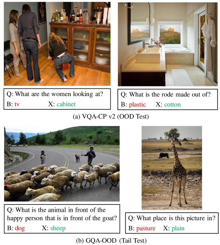
Figure 7. Qualitative examples respectively provided by the Baseline (B), , LXMERT, and the Baseline trained with the X-GGM scheme (X). The wrong and correct answers are highlighted in red and green, respectively.

Vis.

Comparisons with SoTAs on VQA-CP v2. Table 7 shows the full comparisons with state-of-the-art debiasing methods on VQA-CP v2. Compared with both KB-based and UB-based methods, the baseline VQA model (LXMERT) trained with the proposed X-GGM scheme can achieve state-of-the-art OOD and ID performance on VQA-CP v2 “Other”, further demonstrating the effectiveness of X-GGM to OOD generalization.

Additional Qualitative Examples. Like Figure 6, Figure 7 shows some additional qualitative examples from the OOD test set of VQA-CP v2 and GQA-OOD provided by the Baseline (, LXMERT) and the Baseline trained with the X-GGM scheme.

Visualization of Relation Matrix. To further illustrate the process of graph generative modeling, considering the direct relation generation (, R-GGM), Figure 8 compares the head maps of the pre-defined relation matrix ${\bm{R}}_{GT}$ and the generated relation matrix ${\bm{R}}_{g}$ of images which originate from the test set of GQA-OOD in Figure 6 and Figure 7. From the comparison between the heat maps of the pre-fined relation matrix and the generated one, we observe that correlations between nodes becomes more discriminative and new correlations are yielded after R-GGM.

Table 7. Comparisons with state-of-the-art debiasing methods on VQA-CP v2. ^†: methods using additional manually annotated data, ^∗: results from our reimplementation using the official released code, —: not reported.

Method	VQA-CP v2 (OOD Test) $\uparrow$				VQA-CP v2 (ID Test) $\uparrow$				Gap $\downarrow$
	All	Yes/No	Num.	Other	All	Yes/No	Num.	Other	All	Yes/No	Num.	Other
KB-based Methods
RankVQA (Qiao et al., 2020)	43.05	42.53	13.19	51.32	—	—	—	—	—	—	—	—
LM (Clark et al., 2019)	48.78	72.78	14.61	45.58	—	—	—	—	—	—	—	—
LMH (Clark et al., 2019)	52.01	72.58	31.12	46.97	—	—	—	—	—	—	—	—
+ LRS (Guo et al., 2020)	53.26	72.82	48.00	44.46	—	—	—	—	—	—	—	—
+ CCB+VQ-CSS (Yang et al., 2020a)	59.12	89.12	51.04	45.62	—	—	—	—	—	—	—	—
+ MFE (Gat et al., 2020)	54.55	74.03	49.16	45.82	—	—	—	—	—	—	—	—
+ CSS+CL (Liang et al., 2020)	59.18	86.99	49.89	47.16	—	—	—	—	—	—	—	—
+ CSS+GS (Teney et al., 2020a; Liang et al., 2020)	57.37	79.71	50.85	47.45	—	—	—	—	—	—	—	—
+ CSS (Chen et al., 2020b)	58.95	84.37	49.42	48.21	—	—	—	—		—	—	—
+ CCB (Yang et al., 2020a)	57.99	86.41	45.63	48.76	—	—	—	—	—	—	—	—
+ MCE (LXMERT) (Clark et al., 2020)	70.32	—	—	—	70.78	—	—	—	0.46	—	—	—
UB-based Methods
GVQA (Agrawal et al., 2018)	31.30	57.99	13.68	22.14	—	—	—	—	—	—	—	—
Actively Seeking (Teney and Hengel, 2019)	46.00	58.24	29.49	44.33	—	—	—	—	—	—	—	—
Unshuffling+CF+GS (Teney et al., 2020a)	46.80	64.50	15.30	45.90	62.40	77.80	43.80	53.60	15.60	13.30	28.50	7.70
Unshuffling+CF (Teney et al., 2020a)	40.60	61.30	15.60	46.00	63.30	79.40	45.50	53.70	22.70	18.10	29.90	7.70
VGQE (KV and Mittal, 2020)	50.11	66.35	27.08	46.77	—	—	—	—	—	—	—	—
Unshuffling (Teney et al., 2020b)	42.39	47.72	14.43	47.24	—	—	—	—	—	—	—	—
UpDn (Anderson et al., 2018)	38.82	42.98	12.18	43.95	64.73	79.45	49.59	55.66	25.91	36.47	37.41	11.71
+ Top answer masked (Teney et al., 2020c)	40.61	82.44	27.63	22.26	30.90	44.12	5.00	20.85	9.71	38.32	22.63	1.41
+ AdvReg (Grand and Belinkov, 2019)	36.33	59.33	14.01	30.41	50.63	67.39	38.81	38.37	14.30	8.06	24.80	7.96
+ GRL (Grand and Belinkov, 2019)	42.33	59.74	14.78	40.76	56.90	69.23	42.50	49.36	14.57	9.49	27.72	8.60
+ RUBi (Cadene et al., 2019)	47.11	68.65	20.28	43.18	—	—	—	—	—	—	—	—
+ RandImg ($\lambda$=12) (Teney et al., 2020c)	55.37	83.89	41.60	44.20	54.24	64.22	34.40	50.46	1.13	19.67	7.20	6.26
+ CF-VQA (Sum) (Niu et al., 2020)	53.69	91.25	12.80	45.23	—	—	—	—	—	—	—	—
+ CF-VQA (Har.) (Niu et al., 2020)	49.94	74.82	18.93	45.42	—	—	—	—	—	—	—	—
+ DLR (Jing et al., 2020b)	48.87	70.99	18.72	45.57	—	—	—	—	—	—	—	—
+ RandImg ($\lambda$=5) (Teney et al., 2020c)	51.15	75.06	24.30	45.99	59.28	70.66	43.06	53.40	8.13	4.40	18.76	7.41
+ HINT(HAT)† (Selvaraju et al., 2019)	47.70	70.04	10.68	46.31	—	—	—	—	—	—	—	—
+ SCR (HAT)† (Wu and Mooney, 2019)	49.17	71.55	10.72	47.49	—	—	—	—	—	—	—	—
+ SCR (VQA-X)† (Wu and Mooney, 2019)	49.45	72.36	10.93	48.02	—	—	—	—	—	—	—	—
+ SL (Zhu et al., 2020a)	57.59	86.53	29.87	50.03	—	—	—	—	—	—	—	—
+ MUTANT† (Gokhale et al., 2020)	61.72	88.90	49.68	50.78	—	—	—	—	—	—	—	—
+ X-GGM	45.71	43.48	27.65	52.34	67.16	83.74	48.26	56.91	21.45	40.26	20.61	4.57
MANGO (Li et al., 2020)	52.76	—	—	—	—	—	—	—	—	—	—	—
LXMERT∗ (Tan and Bansal, 2019)	63.90	80.45	46.58	59.98	75.57	91.39	59.83	65.21	11.67	10.94	13.25	5.23
+ MUTANT† (Gokhale et al., 2020)	69.52	93.15	67.17	57.78	—	—	—	—	—	—	—	—
+ VILLA∗ (Gan et al., 2020)	48.06	42.66	18.97	58.89	75.85	90.40	60.02	66.66	27.79	47.97	41.05	7.77
+ MCE+Adv (Clark et al., 2020)	66.08	—	—	—	77.17	—	—	—	11.09	—	—	—
+ MCE (Clark et al., 2020)	68.44	—	—	—	74.03	—	—	—	5.59	—	—	—
+ X-GGM	66.95	78.91	53.63	64.33	75.88	90.18	60.06	66.92	8.93	11.27	6.43	2.59

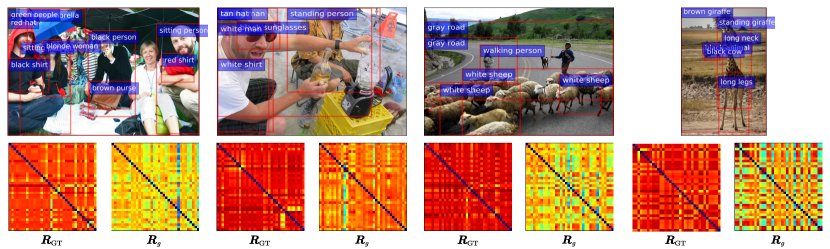
Figure 8. Heat maps of relation matrices. ${\bm{R}}_{GT}$ is the pre-defined relation matrix (, the cosine similarity between object-class embeddings and object-attribute embeddings on the image), ${\bm{R}}_{g}$ is the generated relation matrix during R-GGM.

Vis.