Moving vortices in anisotropic superconductors

Abstract

The magnetic field of moving vortices in anisotropic superconductors is considered in the framework of time-dependent London approach. It is found that at distances large relative to the core size, the field may change sign that alludes to a non-trivial intervortex interaction which depends on the crystal anisotropy and on the speed and direction of motion. These effects are caused to the electric fields and corresponding normal currents which appear due to the moving vortex magnetic structure. We find that the motion related part of the magnetic field attenuates at large distances as $1/r^{3}$ unlike the exponential decay of the static vortex field. The electric field induced by the vortex motion decreases as $1/r^{2}$.

I Introduction

The problem of interaction of vortices in anisotropic superconductors has been studied extensively in early 90s both theoretically Grishin ; Buzdin ; NakThiem and experimentally Bolle . For vortices parallel to one of the principal crystal directions the problem is solved just by rescaling the isotropic results. In particular the interaction is repulsive for any position of the second vortex relative to the first. However, the force direction in general is not along the vector $\bm{R}$ connecting the vortices, in other words, for an arbitrary positions of the pair there is a torque, unless $\bm{R}$ is directed along principal directions forces .

The situation is different if parallel vortices are tilted out of principal directions Grishin ; Buzdin ; NakThiem . Then, at distances of the order of London penetration depth $\lambda$, the magnetic field $\bm{h}(\bm{R})$ of a single tilted vortex may change sign and approach zero for $R\to\infty$ being negative. In other words, the vortex-vortex interaction being repulsive at short distances may turn attractive at large distances. This leads to formation of chains of vortices in tilted fields Bolle .

In this paper we consider the magnetic field and current distributions of moving anisotropic vortices. Commonly, moving vortices are considered as static but displaced as a whole. It was argued, however, that out-of-core moving vortex structure differs from the static case due to out-of-core dissipation leo ; TDL . The moving vortex magnetic field $h(r,t)$ generates the electric field and currents of normal excitations, which in turn distort the field $h$. We show that at large distances the distortion is not small and even able to change the field sign. Unexpectedly, this distortion attenuates with distance as a power law $1/R^{3}$, i.e. much slower than the standard decay of undistorted field $\sim e^{-R/\lambda}$.

At distances large in comparison to the core size of interest in this work, one can use the time-dependent London approach based on the assumption that the current consists of the normal and superconducting parts:

$${\bm{J}}=\sigma{\bm{E}}-\frac{2e^{2}|\Psi|^{2}}{mc}\,\left({\bm{A}}+\frac{\phi_{0}}{2\pi}{\bm{\nabla}}\chi\right)\,,$$ (1)

where $\bm{A}$ is the vector potential, $\Psi$ is the order parameter, $\chi$ is the phase, $\phi_{0}$ is the flux quantum, ${\bm{E}}$ is the electric field, and $\sigma$ is the conductivity associated with normal excitations.

The conductivity $\sigma$ approaches the normal state value $\sigma_{n}$ when the temperature $T$ approaches $T_{c}$; in s-wave superconductors it vanishes with decreasing temperature along with the density of normal excitations. This is not the case, however, for strong pair-breaking when superconductivity is gapless while the density of states approaches the normal state value at all temperatures. Unfortunately, not much experimental information about the $T$ dependence of $\sigma$ is available. Theoretically, this question is still debated, e.g. Ref. Andreev discusses possible enhancement of $\sigma$ due to inelastic scattering. Experimentally, interpretation of the microwave absorption data is not yet settled either Maeda .

At distances large in comparison with the vortex core size, $|\Psi|$ is a constant $\Psi_{0}$ and Eq. (1) becomes:

$$\frac{4\pi}{c}{\bm{J}}=\frac{4\pi\sigma}{c}{\bm{E}}-\frac{1}{\lambda^{2}}\,\left({\bm{A}}+\frac{\phi_{0}}{2\pi}{\bm{\nabla}}\chi\right)\,,$$ (2)

where $\lambda^{2}=mc^{2}/8\pi e^{2}|\Psi_{0}|^{2}$ is the London penetration depth. Acting on this by curl one obtains:

$${\bm{h}}-\lambda^{2}\nabla^{2}{\bm{h}}+\tau\,\frac{\partial{\bm{h}}}{\partial t}=\phi_{0}{\bm{z}}\sum_{\nu}\delta({\bm{r}}-{\bm{r}_{\nu}})\,,$$ (3)

where ${\bm{r}_{\nu}}(t)$ is the position of the $\nu$-th vortex which may depend on time $t$, $\bm{z}$ is the direction of vortices, and the relaxation time

$$\tau=4\pi\sigma\lambda^{2}/c^{2}\,.$$ (4)

Equation (3) can be considered as a general form of the time dependent London equation (TDL). The anisotropic generalization of this equation was given in anisTDL and reproduced here in Section III.

II Vortex at rest in anisotropic case

For an arbitrary oriented vortex in anisotropic material this problem have been considered in K81 ; Grishin . In general, results are cumbersome, so here we consider a simple situation of an orthorhombic superconductor in field along the $c$ axis. The London equation in this case is:

$$h_{z}(x,y)-\lambda^{2}_{1}\,\frac{\partial^{2}h_{z}}{\partial y^{2}}-\lambda^{2}_{2}\,\frac{\partial^{2}h_{z}}{\partial x^{2}}=\phi_{0}\delta(\bm{r})\,,$$ (5)

Here, the frame $x,y,z$ is chosen to coincide with $a,b,c$ of the crystal, $\bm{r}=(x,y)$, $\lambda^{2}_{xx}=\lambda^{2}_{1}$ and $\lambda^{2}_{yy}=\lambda^{2}_{2}$ are the diagonal components of the tensor $(\lambda^{2})_{ik}$. The solution of this equation is

$$h_{z}(x,y)=\frac{\phi_{0}}{2\pi\lambda_{1}\lambda_{2}}K_{0}\left(\rho\right)\,,\quad\rho^{2}=\frac{x^{2}}{\lambda_{2}^{2}}+\frac{y^{2}}{\lambda_{1}^{2}}\,.$$ (6)

Current densities follow:

$$J_{x}=-\frac{c\phi_{0}}{8\pi^{2}\lambda_{1}^{3}\lambda_{2}}\frac{y\,K_{1}(\rho)}{\rho}\,,\quad J_{y}=\frac{c\phi_{0}}{8\pi^{2}\lambda_{1}\lambda_{2}^{3}}\frac{x\,K_{1}(\rho)}{\rho}\,,\qquad$$ (7)

where $K_{0,1}$ are Modified Bessel functions.

It is easy to see that the contours $h_{z}(x,y)=\,\,$const coincide with the stream lines of the current, an example is shown in Fig. 1.

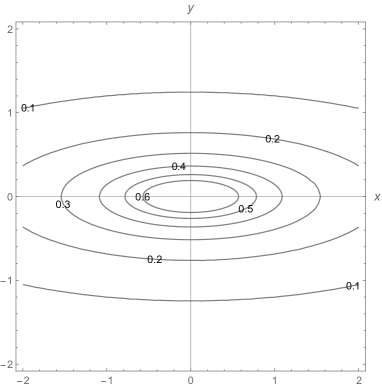
Figure 1: The stream lines of the current for $\gamma=\lambda_{2}/\lambda_{1}=3$ or, which is the same, contours of constant $h_{z}(x,y)$. $\lambda_{1}$ is taken as unit length.

The current lines have the expected ellipse-like shape.

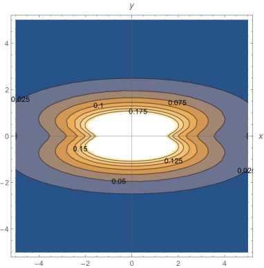
Figure 2: The contours of constant current values $J(x,y)=\sqrt{J_{x}^{2}+J_{y}^{2}}$ for $\lambda_{2}/\lambda_{1}=3$. $x$ and $y$ are in units of $\lambda_{1}$.

This is, however, not the case for the distribution of the current values $J(x,y)=\sqrt{J_{x}^{2}+J_{y}^{2}}$. An example is shown in Fig. 2. Hence, the geometry of the streamlines of the vector $\bm{J}$ differs from that of contours $|J(x,y)|=const$, unlike the isotropic case where they are in fact the same.

III Moving vortex

The anisotropic generalization of the isotropic Eq. (2) for the current is straightforward:

$$J_{k}=\sigma_{kl}E_{l}-\frac{c}{4\pi}\left(\lambda^{-2}\right)_{kl}\left(A_{l}+\frac{\phi_{0}}{2\pi}\frac{\partial\chi}{\partial x_{l}}\right)\,.$$ (8)

Here, $\sigma_{kl}$ and $\left(\lambda^{-2}\right)_{kl}$ are tensors of the conductivity due to normal excitations and of the inverse square of the penetration depth.

Having in mind to derive an equation for the magnetic field $\bm{h}$ we first have to get rid of the vector potential. To this end, multiply both sides by $4\pi\left(\lambda^{2}\right)_{k\mu}/c$ where $\left(\lambda^{2}\right)_{k\mu}$ is the tensor inverse to $\left(\lambda^{-2}\right)_{k\mu}$ and sum up over $k$. Then apply ${\rm curl}$ to both sides and use the relation

$${\rm curl}(\bm{A}+\phi_{0}\bm{\nabla}\chi/2\pi)=\bm{h}-\phi_{0}\hat{\bm{z}}\delta(\bm{r}-\bm{r}_{\nu})\,,$$ (9)

where $\bm{r}_{\nu}$ is the vortex core position.

It is convenient to use in the following the notation curl${}_{\nu}\bm{V}=\epsilon_{\nu s\mu}\partial V_{\mu}/\partial x_{s}$ where $\epsilon_{\nu s\mu}$ is Levi-Chivita unit antisymmetric tensor: $\epsilon_{xyz}=1$ and so do all components with even number of transpositions of indices, it is $-1$ for odd numbers, and zero otherwise.

Hence, applying $\epsilon_{\nu s\mu}\partial/\partial x_{s}$ to Eq. (8), one obtains the anisotropic version of TDL anisTDL :

$$h_{\nu} + \frac{4\pi}{c}\epsilon_{\nu s\mu}\lambda^{2}_{k\mu}\frac{\partial J_{k}}{\partial x_{s}}-\frac{4\pi}{c}\epsilon_{\nu s\mu}\lambda^{2}_{k\mu}\sigma_{kl}\frac{\partial E_{l}}{\partial x_{s}}$$ (10)

$$= \phi_{0}\hat{\bm{z}}_{\nu}\delta(\bm{r}-\bm{v}t).\qquad$$

In this form, the equation is valid for an arbitrary oriented vortex and any crystal anisotropy.

For an orthorhombic crystal in which the vortex and its field are along one of the principal directions (call it $z$), this cumbersome equation takes the form:

$$h_{z} - \frac{4\pi}{c}\left(\lambda^{2}_{xx}\frac{\partial J_{x}}{\partial y}-\lambda^{2}_{yy}\frac{\partial J_{y}}{\partial x}\right)$$ (11)

$$+ \frac{4\pi\sigma}{c}\left(\lambda^{2}_{xx}\frac{\partial E_{x}}{\partial y}-\lambda^{2}_{yy}\frac{\partial E_{y}}{\partial x}\right)=\phi_{0}\delta(\bm{r}-\bm{v}t).\qquad$$

Here we further simplified the problem assuming isotropic conductivity of normal excitations $\sigma_{xx}=\sigma_{yy}=\sigma$. This should be solved together with quasi-stationary Maxwell equations curl$\bm{E}=-\partial_{t}\bm{h}/c$ and div$\bm{E}=0$ LL ; Gorkov , which can be done in 2D Fourier space:

$$E_{\bm{k}x}=-\frac{k_{y}}{k_{x}}E_{\bm{k}y}=-\frac{ik_{y}}{ck^{2}}\,\frac{\partial h_{\bm{k}z}}{\partial t}\,,$$ (12)

so that we obtain the 2D Fourier transform of Eq. (11):

$$h_{\bm{k}} \left(1+k_{x}^{2}\lambda^{2}_{yy}+k_{y}^{2}\lambda^{2}_{xx}\right)$$ (13)

$$+\frac{4\pi\sigma}{c^{2}}\,\frac{\lambda^{2}_{yy}k_{x}^{2}+\lambda^{2}_{xx}k_{y}^{2}}{k^{2}}\frac{\partial h_{\bm{k}}}{\partial t}=\phi_{0}e^{-i\bm{k}\bm{v}t}\,,$$

where $h_{\bm{k}}$ is the Fourier transform of $h_{z}(\bm{r})$. In isotropic case we obtain the equation studied in TDL . We further denote $\lambda^{2}_{yy}=\lambda_{2}^{2},\quad\lambda^{2}_{xx}=\lambda_{1}^{2}$ and $\lambda=\sqrt{\lambda_{1}\lambda_{2}}$. The anisotropy parameter is defined as $\gamma=\lambda_{2}/\lambda_{1}$. Then, we obtain:

$$h_{\bm{k}}\left(1+k_{x}^{2}\lambda^{2}_{2}+k_{y}^{2}\lambda^{2}_{1}\right)+\tau\,\frac{\lambda^{2}_{2}k_{x}^{2}+\lambda^{2}_{1}k_{y}^{2}}{\lambda^{2}k^{2}}\frac{\partial h_{\bm{k}}}{\partial t}=\phi_{0}e^{-i\bm{k}\bm{v}t}.$$

(14)

with $\tau=4\pi\sigma\lambda^{2}/c^{2}$. This is a linear differential equation for $h_{\bm{k}}(t)$ with the solution

$$h_{\bm{k}}=\frac{\phi_{0}e^{-i\bm{k}\bm{v}t}}{C-iD\bm{k}\cdot\bm{s}}\,,\quad\bm{s}=\bm{v}\tau\,,$$

$$C=1+k_{x}^{2}\lambda^{2}_{2}+k_{y}^{2}\lambda^{2}_{1}\,,\quad D=\frac{\lambda^{2}_{2}k_{x}^{2}+\lambda^{2}_{1}k_{y}^{2}}{\lambda^{2}k^{2}}\,.\qquad$$ (15)

Since we are interested in stationary motion with a constant velocity, we can set here $t=0$.

The dimensionless parameter

$$S=\frac{s}{\lambda}=\frac{4\pi v\sigma\lambda}{c^{2}}$$ (16)

is small even for vortex velocities exceeding the speed of sound presently attainable Eli ; Denis . Although in principle $S$ can take larger values, we restrict this discussion by small $S$ and call this case a “slow motion”.

IV Slow motion

For $s\to 0$ one can expand $h(\bm{k},\bm{s})$ in powers of small $s$ up to ${\cal O}(s)$:

$$h_{\bm{k}}=\frac{\phi_{0}}{C}+i\frac{\phi_{0}D}{C^{2}}\bm{k}\cdot\bm{s}\,,$$ (17)

The first term corresponds to the static solution discussed above:

$$h_{0}(x,y)=\frac{\phi_{0}}{2\pi\lambda^{2}}K_{0}\left(\rho\right)\,,\quad\rho^{2}=\frac{x^{2}}{\lambda_{2}^{2}}+\frac{y^{2}}{\lambda_{1}^{2}}\,.$$ (18)

The correction due to motion is given by

$$\frac{\delta h_{\bm{k}}\lambda^{2}}{\phi_{0}}=i\frac{(\lambda^{2}_{2}k_{x}^{2}+\lambda^{2}_{1}k_{y}^{2})\bm{k}\cdot\bm{s}}{k^{2}(1+\lambda^{2}_{2}k_{x}^{2}+\lambda^{2}_{1}k_{y}^{2})^{2}}\,,$$ (19)

To separate the part that does not disappear when $\lambda_{1}=\lambda_{2}$, one can use the identity

$$\frac{\lambda^{2}_{2}k_{x}^{2}+\lambda^{2}_{1}k_{y}^{2}}{k_{x}^{2}+k_{y}^{2}}=\lambda_{2}^{2}+\frac{k_{y}^{2}(\lambda^{2}_{1}-\lambda^{2}_{2})}{k_{x}^{2}+k_{y}^{2}}$$ (20)

to obtain:

$$\frac{4\pi^{2}\lambda^{2}\delta h(\bm{r})}{i\phi_{0}}=\lambda_{2}^{2}\int\frac{d^{2}\bm{k}(\bm{k}\cdot\bm{s})e^{i\bm{k}\bm{r}}}{(1+\lambda^{2}_{2}k_{x}^{2}+\lambda^{2}_{1}k_{y}^{2})^{2}}$$

$$+(\lambda^{2}_{1}-\lambda^{2}_{2})\int\frac{d^{2}\bm{k}k_{y}^{2}(\bm{k}\cdot\bm{s})e^{i\bm{k}\bm{r}}}{k^{2}(1+\lambda^{2}_{2}k_{x}^{2}+\lambda^{2}_{1}k_{y}^{2})^{2}}\,.$$ (21)

Evaluation of the first contribution is outlined in Appendix A:

$$h_{1}=-\frac{\phi_{0}}{2\pi\lambda^{2}}\frac{S_{x}X+S_{y}Y\gamma^{2}}{2}K_{0}\left(\sqrt{\frac{X^{2}}{\gamma}+Y^{2}\gamma}\right)\,,\qquad$$ (22)

where

$$\bm{S}=\frac{\bm{s}}{\lambda},\,\,\,X=\frac{x}{\lambda},\,\,\,Y=\frac{y}{\lambda},\,\,\,\lambda=\sqrt{\lambda_{1}\lambda_{2}},\,\,\,\gamma=\frac{\lambda_{2}}{\lambda_{1}}.\qquad$$ (23)

It is shown in Norio2 that in the isotropic case for a vortex moving along $x$

$$h(\bm{r})=\frac{\phi_{0}}{2\pi\lambda^{2}}e^{-sx/2\lambda^{2}}K_{0}\left(\frac{r}{2\lambda}\sqrt{4+s^{2}/\lambda^{2}}\right)\qquad$$ (24)

in common units. Expanding this in small $s$ one obtains for a slow motion:

$$\delta h(\bm{r})=-\frac{\phi_{0}}{4\pi\lambda^{4}}sxK_{0}\left(\frac{r}{\lambda}\right)\,.$$ (25)

Hence, $h_{1}$ of Eq. (22) has the correct isotropic limit.

The second integral over two components of $\bm{k}$ in Eq. (21) can be reduced to integrals over a single variable which are easy to deal with numerically, see Appendix B:

$$\frac{2\pi\lambda^{2}}{\phi_{0}}h_{2}=\frac{(\gamma^{2}-1)}{4\gamma}\Big{\{}S_{x}X\int_{0}^{\infty}\frac{d\zeta}{(\zeta+\gamma)^{3/2}(\zeta+1/\gamma)^{3/2}}\left[K_{0}\left({\cal R}_{\zeta}\right)-\frac{Y^{2}}{(\zeta+1/\gamma){\cal R}_{\zeta}}K_{1}\left({\cal R}_{\zeta}\right)\right]$$

$$+S_{y}Y\int_{0}^{\infty}\frac{d\zeta}{(\zeta+\gamma)^{1/2}(\zeta+1/\gamma)^{5/2}}\left[3K_{0}\left({\cal R}_{\zeta}\right)-\frac{Y^{2}}{(\zeta+1/\gamma){\cal R}_{\zeta}}K_{1}\left({\cal R}_{\zeta}\right)\right]\Big{\}},\qquad{\cal R}_{\zeta}=\sqrt{\frac{X^{2}}{\zeta+\gamma}+\frac{Y^{2}}{\zeta+1/\gamma}}\,.\qquad\qquad\qquad\qquad$$ (26)

Thus, the vortex field can be calculated as $h=h_{0}+h_{1}+h_{2}$ with $h_{0}$ given in Eq. (18), $h_{1}$ in Eq. (22), and $h_{2}$ in Eq. (26). The results obtained with the help of Wolfram Mathematica package are shown below.

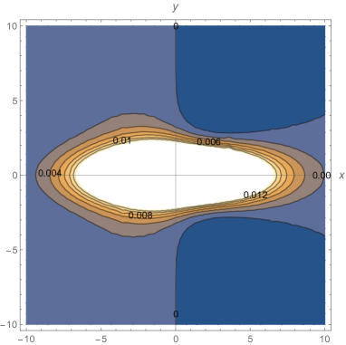
Figure 3: Contours $h(x,y)=$ const for the vortex moving along $x$ axis ($S_{x}=0.1,\,\,S_{y}=0$) and $\lambda_{2}/\lambda_{1}=3$. The motion is directed to $+x$. $x$ and $y$ are in units of $\lambda=\sqrt{\lambda_{1}\lambda_{2}}$.

One can see in Fig. 3 that the current stream-lines (or, what is the same, contours $h(x,y)=$ const) in the vicinity of the moving vortex core are only weakly distorted relative to the static elliptic shape. The most interesting feature of this distribution is that at large distances $h(x,y)$ changes sign in some parts of the $(x,y)$ plane. Since the interaction energy of the vortex at the origin with another one at $(x,y)$ is proportional to $h(x,y)$, the presence of domains with $h<0$ means that for the second vortex in these domains the intervortex interaction is attractive.

The field distribution is different for the motion along $y$ axis shown in Fig. 4.

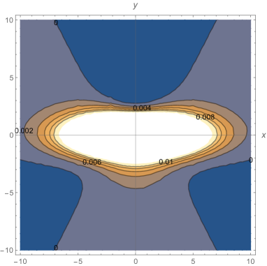
Figure 4: Contours $h(x,y)=$ const for the vortex moving along $y$ axis ($S_{x}=0,S_{y}=0.1$) and $\lambda_{2}/\lambda_{1}=3$. The motion is directed to $+y$. $x$ and $y$ are in units of $\lambda=\sqrt{\lambda_{1}\lambda_{2}}$.

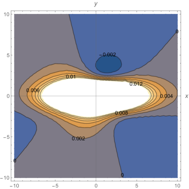
Figure 5: Contours $h(x,y)=$ const for the vortex moving along the diagonal $x=y$ ($S_{x}=S_{y}=0.1$) and $\lambda_{2}/\lambda_{1}=3$. $x$ and $y$ are in units of $\lambda=\sqrt{\lambda_{1}\lambda_{2}}$.

It is seen that the flux in front of the moving vortex is depleted whereas behind it is enhanced, the feature first discussed in norio1 for the isotropic case. This feature remains also for a general direction of motion; an example of motion along the line $x=y$ is shown in Fig. 5. Moreover, Fig. 3–5 show that this depletion may even change sign of the field.

It is worth mentioning that the London theory is reliable in the region $r\gg\xi$, $\xi$ being the core size, and so are our predictions of a non-trivial behavior of $h(x,y)$ at large distances.

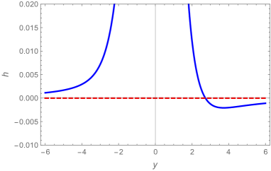
Figure 6: The field $h(0,y)$ for the vortex moving along $y$ ($S_{x}=0,S_{y}=0.1$); $\lambda_{2}/\lambda_{1}=3$. $x$ is in units of $\lambda=\sqrt{\lambda_{1}\lambda_{2}}$.

It is instructive to see how the interaction changes along certain directions. E.g., for $S_{x}=0,\,\,\,S_{y}=0.1$, the motion along $y$-axis, $h(0,Y)$ is positive if $0<Y\lesssim 2.5$ (so that the second vortex at $(0,Y)$ in this region is repelled by the vortex at the origin). If the second vortex is at $2.5\lesssim Y<\infty$ the interaction is attractive. This is illustrated in Fig. 6.

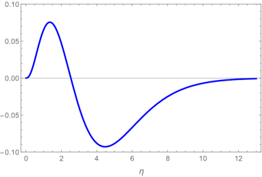
Figure 7: The integrand of Eq. (28) for $Y=10$ and $\gamma=3$.

IV.1 Asymptotic behavior of $\bm{h(0,Y)}$ for $\bm{Y\to\infty}$

For $X=0$, Eq. (26) yields

$$\frac{2\pi\lambda^{2}}{\phi_{0}}h_{2}=\frac{\gamma^{2}-1}{4\gamma}S_{y}Y\int_{0}^{\infty}\frac{d\zeta\left[3K_{0}(\eta)-\eta K_{1}(\eta)\right]}{(\zeta+\gamma)^{1/2}(\zeta+1/\gamma)^{5/2}},$$

$$\eta=\frac{|Y|}{\sqrt{\zeta+1/\gamma}}\,.\qquad\qquad\qquad\qquad$$ (27)

Going to the integration variable $\eta$, we get

$$\frac{2\pi\lambda^{2}}{\phi_{0}}h_{2}=\frac{\gamma^{2}-1}{2\gamma}\frac{S_{y}}{Y^{2}}\int_{0}^{Y\sqrt{\gamma}}\frac{d\eta\,\eta^{3}\left[3K_{0}(\eta)-\eta K_{1}(\eta)\right]}{\sqrt{Y^{2}+\eta^{2}(\gamma-1/\gamma)}}.$$

(28)

Fig. 7 shows that the integrand here is substantial only in the finite region $0<\eta\lesssim 10$. Therefore being interested in the asymptotic behavior for $|Y|\to\infty$, one can replace the denominator by $|Y|$ and the upper limit of integration by $\infty$:

$$\frac{2\pi\lambda^{2}}{\phi_{0}}h_{2}(0,Y) = \frac{\gamma^{2}-1}{2\gamma}\frac{S_{y}}{Y^{3}}\int_{0}^{\infty}d\eta\,\eta^{3}\left[3K_{0}-\eta K_{1}\right]_{\eta}\qquad$$ (29)

$$= -\frac{\gamma^{2}-1}{\gamma}\frac{2S_{y}}{Y^{3}}\,.$$

Thus, $h_{2}(0,Y)$ is negative when $Y\to\infty$ and positive for $Y\to-\infty$. It decays as $1/Y^{3}$, therefore, the total field $h_{0}+h_{1}+h_{2}$ attenuates as a power law as well, since $h_{0}$ and $h_{1}$ decay exponentially and at large distances can be disregarded. Hence, $h_{2}$ can be replaced with $h$ in this region. This conclusion agrees with direct numerical evaluation of $h(0,Y)$ shown in Fig. 6

In the same way one can obtain the leading term in the asymptotic behavior for $Y=S_{y}=0$ for the motion along the $x$ axis:

$$h(X,0)\sim\frac{\phi_{0}}{2\pi\lambda^{2}}\frac{\gamma^{2}-1}{2\gamma}\frac{2S_{x}}{X^{3}}\,.$$ (30)

For the sake of brevity we do not provide other terms in the asymptotic series.

The power-law decay of the field $h(x,y)$ for vortices moving in anisotropic superconductors is a surprising feature. Clearly, this feature disappears for vortices at rest as well as for vortices moving in isotropic materials. Formally, the power-law behavior in real space originates in the factor $1/k^{2}$ in Fourier transforms, see e.g. Eq. (21), which, however, cancels out for $\gamma=1$.

V Electric field for slow motion

In the approximation linear in velocity, we have according to Eq. (15)

$$\frac{\partial h_{\bm{k}}}{\partial t}=-i\frac{\phi_{0}(\bm{k}\cdot\bm{v})}{C}\,,\quad C=1+k_{x}^{2}\lambda^{2}_{2}+k_{y}^{2}\lambda^{2}_{1}\,.$$ (31)

This yields the electric field

$$E_{\bm{k}x}=-\frac{k_{y}}{k_{x}}E_{\bm{k}y}=-\frac{\phi_{0}}{c\tau}\frac{k_{y}(\bm{k}\cdot\bm{s})}{k^{2}C}\,,\quad\bm{s}=\bm{v}\tau\,,$$ (32)

see Eqs. (12). Hence, we have in real space

$$E_{x}=-\frac{\phi_{0}}{4\pi^{2}c\tau}\int\frac{d^{2}\bm{k}\,k_{y}(\bm{k}\cdot\bm{s})}{k^{2}C}e^{i\bm{k}\bm{r}}\,,$$ (33)

or, using $\lambda=\sqrt{\lambda_{1}\lambda_{2}}$ as the unit length,

$$E_{x}=-\frac{\phi_{0}}{4\pi^{2}c\tau\lambda}\int\frac{d^{2}\bm{q}\,q_{y}(\bm{q}\cdot\bm{S})}{q^{2}C}e^{i\bm{q}\bm{R}}\,.$$ (34)

Here, $\bm{q}=\bm{k}\lambda$, $\bm{R}=(X,Y)=\bm{r}/\lambda$ (see definitions (23), and

$$C=1+q_{x}^{2}\gamma+q_{y}^{2}/\gamma\,,\quad\gamma=\lambda_{2}/\lambda_{1}\,.$$ (35)

In the same way we obtain

$$E_{y}=\frac{\phi_{0}}{4\pi^{2}c\tau\lambda}\int\frac{d^{2}\bm{q}\,q_{x}(\bm{q}\cdot\bm{S})}{q^{2}C}e^{i\bm{q}\bm{R}}\,.$$ (36)

The integrals in Eqs. (34) and (36) are dimensionless.

It is of interest to see the streamlines of $\bm{E}$ (or, that is the same, of the normal current $\bm{J}_{n}=\sigma\bm{E}$). To this end, we calculate the stream function $G(x,y)$ such that $E_{x}=\partial_{y}G$ and $E_{y}=-\partial_{x}G$; the streamlines then are given by contours $G(x,y)=const$. In Fourier space we have $E_{x\bm{k}}=ik_{y}G_{\bm{k}}$ so that

$$G_{\bm{k}}=\frac{i\phi_{0}}{c\tau}\frac{(\bm{k}\cdot\bm{s})}{k^{2}C},\,\,\,\,G(\bm{r})=\frac{i\phi_{0}}{4\pi^{2}c\tau}\int\frac{d^{2}\bm{q}(\bm{q}\cdot\bm{S})e^{i\bm{q}\bm{R}}}{q^{2}C}.\qquad$$ (37)

The formal procedure of reducing the double to single integration in Eq. (37) is similar to that used for $h(\bm{r})$ and is outlined in Appendix C. The result is:

$$G(\bm{r})=-\frac{\phi_{0}}{4\pi c\tau}\int_{0}^{\infty}\frac{d\eta\,K_{0}({\cal R}\sqrt{\eta})}{\sqrt{\mu\nu}}\left(\frac{S_{x}X}{\mu}+\frac{S_{y}Y}{\nu}\right),$$

$$\mu=1+\eta\gamma\,,\quad\nu=1+\eta/\gamma\,,\quad{\cal R}=\sqrt{\frac{X^{2}}{\mu}+\frac{Y^{2}}{\nu}}\,.\qquad$$ (38)

Figs. 8 and 9 show two examples of $J_{n}$-streamlines (or contours $G(X,Y)=\,\,$const) obtained by numerical integration of Eq. (38).

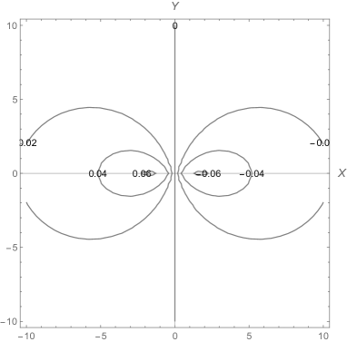
Figure 8: Streamlines of the field $\bm{E}$ (or of the normal current $\bm{J}_{n}$) for the vortex moving along $X$ ($S_{x}=0.1,S_{y}=0$). $\gamma=\lambda_{2}/\lambda_{1}=3$. $X,Y$ are in units of $\lambda=\sqrt{\lambda_{1}\lambda_{2}}$. Positive constants by the contours correspond to the clockwise current direction, negative otherwise.

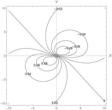
Figure 9: Streamlines of the normal current for the vortex moving along the line $X=Y$ ($S_{x}=S_{y}=0.1$), $\gamma=\lambda_{2}/\lambda_{1}=3$. $X,Y$ are in units of $\lambda=\sqrt{\lambda_{1}\lambda_{2}}$. Positive constants by the contours correspond to the clockwise current direction, negative otherwise.

The electric field is now readily obtained by differentiation of $G$. We will not write down these cumbersome expressions. Instead we consider the asymptotic behavior of electric fields at large distances in two relatively simple cases using the method employed above for asymptotic behavior of $h(0,y)$ and $h(x,0)$. Omitting formalities, we give the results:

$$G(X,0)\sim-\frac{\phi_{0}}{2\pi c\tau}\frac{S_{x}}{X}\,,\qquad|X|\to\infty\,,$$ (39)

that yields

$$E_{x}(X,0)=0\,,\quad E_{y}(X,0)\sim\frac{\phi_{0}}{2\pi c\tau}\frac{S_{x}}{X^{2}}\,.$$ (40)

Similarly, for the motion along $Y$ axis

$$E_{y}(0,Y)=0\,,\quad E_{x}(0,Y)\sim\frac{\phi_{0}}{2\pi c\tau}\frac{S_{y}}{Y^{2}}\,.$$ (41)

Interestingly, the material anisotropy does not enter these results at all. This means that the power-law decay of the electric field should exists also in the isotropic case. In fact, for $\gamma=1$ one has from Eq. (37)

$$G(X,0)=\frac{i\phi_{0}S_{x}}{4\pi^{2}c\tau}\int\frac{d^{2}\bm{q}\,q_{x}e^{i\bm{q}\bm{X}}}{q^{2}(1+q^{2})},\qquad$$ (42)

which is readily done integrating first over the angle between $\bm{q}$ and $\bm{X}$. We obtain:

$$G(X,0)=\frac{\phi_{0}S_{x}}{2\pi c\tau}\left[K_{1}(X)-\frac{1}{X}\right],\qquad$$ (43)

that gives

$$E_{y}(X,0)=-\frac{\phi_{0}S_{x}}{2\pi c\tau}\left[K_{1}^{\prime}(X)+\frac{1}{X^{2}}\right].$$ (44)

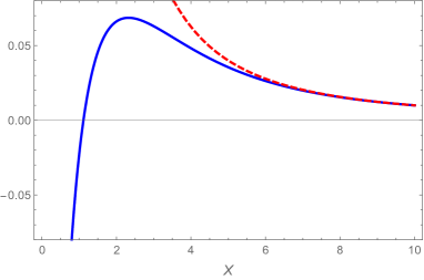
Figure 10: The solid line is the square brackets in Eq. (44) for $E_{y}(X,0)$ when the vortex moves along the $X$ axis ($S_{y}=0$), $\gamma=1$. The dashed line shows the power-law term $1/X^{2}$. $X$ are in units of $\lambda$.

Figure 10 shows that the field $E_{y}(X,0)$ changes sign at $x/\lambda\approx 1$, reaches maximum near 2, and slowly decays as a power law $\lambda^{2}/x^{2}$. This is quite surprising since the electric field power-law decay means that no screening of $\bm{E}$ is involved, in other words, that there is no Meissner-type effect for the field $\bm{E}$.

VI Discussion

We have studied effects of vortex motion within time dependent London theory, which is based on the assumption that in time dependent phenomena the current in superconductors consists of the persistent and normal components, Eq. (2). This approach differs from the common assumption that the vortex magnetic structure moves as a whole, so that in the frame bound to the moving vortex the magnetic field distribution is the same as for a vortex at rest, see e.g. Dolgov or multitude of papers describing the flux flow.

Within the TDL approach the field distribution of the moving vortex differs from that of vortex at rest even in the frame moving with the vortex. The physical reason for this is simple: the moving magnetic structure $h(x,y)$ induces the electric field and currents of normal excitations, while the latter distort the moving static field distribution $h_{0}(x,y)$. This is a general feature of systems with singularities (vortices) moving in dissipative media leo ; TDL . The equation describing these time-dependent phenomena are diffusion-like, so that solutions are obtained in the 2D Fourier space: we obtain $h_{\bm{k}}$ and to recover $h({\bm{r}})$ one has to evaluate double integrals $\int d^{2}\bm{k}...\,$, a heavy numerical procedure. We offer a way to reduce double integrals to a single $\int_{0}^{\infty}d\eta...$ which can be evaluated within Wolfram Mathematica package efficiently and fast, that is relevant especially for generating plots of various 2D distributions.

We have investigated the field distribution of moving vortices away of the vortex core whether the time-dependent London theory is reliable. As in the isotropic case norio1 , the magnetic field of moving vortices in anisotropic materials is distorted relative to the static case, the magnetic flux is redistributed so that it is depleted in front of the moving vortex and enhanced behind it. The depletion could be strong enough so that the field $h_{z}$ changes sign in some parts of the $xy$ plane. This suggests that the interaction of two vortices, one at the origin at some moment and another is at $(x,y)$, being repulsive at short intervortex distances may turn attractive.

The physical reason for this change is the induced electric field $\bm{E}$ and along with it the currents of normal excitations $\sigma\bm{E}$. This field is obtained by solving quasi-stationary Maxwell equations curl$\bm{E}=\partial_{t}\bm{h}/c$, the condition of quasi-neutrality div$\bm{E}=0$, coupled with the time-dependent London equation (basically, the same procedure as in deriving time-dependent Ginzburg-Landau equations Gorkov ). Unlike $\bm{h}$, the field $\bm{E}$ cannot be screened in the bulk of the material, so that one may say that there is no “Meissner effect” for the electric field per se.

It turns out that in anisotropic case the magnetic field of moving vortex has a power law dependence on distances $r>>\lambda$: $h\propto(\gamma^{2}-1)v/r^{3}$ ($\gamma$ is the anisotropy parameter, $v$ is the vortex velocity). The exponentially decaying part of $h$ is still present, but at large distances it is irrelevant in comparison with the power-law part. In isotropic case, the power law gives way to the standard exponential decay. The electric field, however, goes as $1/r^{2}$ in both cases.

Most of our calculation were done for orthorhombic materials with the in-plane anisotropy parameter $\gamma=3$ and the vortex along $c$. Such materials in fact exist, examples are NiBi films NiBi , or Ta₄Pd₃Te₁₆ 17 .

Appendix A

Consider the integral

$$\int\frac{d^{2}\bm{k}e^{i\bm{k}\bm{r}}}{(1+k^{2})^{2}}=\int_{0}^{\infty}\frac{k\,dk}{(1+k^{2})^{2}}\int_{0}^{2\pi}d\varphi e^{ikr\cos(\alpha-\varphi)}=2\pi\int_{0}^{\infty}\frac{k\,dk}{(1+k^{2})^{2}}J_{0}(kr)=\pi rK_{1}(r)\,,$$ (45)

$\bm{k}$ and $\bm{r}$ are at angles $\varphi$ and $\alpha$ relative to $x$. Apply $\partial_{x}$ to both sides:

$$\int\frac{d^{2}\bm{k}k_{x}e^{i\bm{k}\bm{r}}}{(1+k^{2})^{2}}=i\pi xK_{0}(r)\,,$$ (46)

The evaluation of the first integral in Eq. (21) is now straightforward.

Appendix B

The second contribution in Eq. (21) consists of parts related to $x$ and $y$ projection of the velocity. With the help of identities

$$\frac{1}{f}=\int_{0}^{\infty}du\,e^{-fu}\,,\quad\frac{1}{f^{2}}=\int_{0}^{\infty}du\,u\,e^{-fu},\qquad$$ (47)

one recasts the $x$-part:

$$I_{x}=\frac{S_{x}(1-\gamma^{2})}{\gamma}\int\frac{d^{2}\bm{q}\,q_{y}^{2}q_{x}e^{i\bm{q}\bm{R}}}{q^{2}(1+\gamma q_{x}^{2}+q_{y}^{2}/\gamma)^{2}}=\int_{0}^{\infty}d\xi\int_{0}^{\infty}du\,ue^{-u}\int d^{2}\bm{q}\,q_{y}^{2}q_{x}e^{i\bm{q}\bm{R}-(\xi+u\gamma)q_{x}^{2}-(\xi+u/\gamma)q_{y}^{2}}\,.$$ (48)

Here we use $\lambda$ as a unit length: $\bm{q}=\bm{k}\lambda$, $\bm{R}=\bm{r}/\lambda$$,\lambda_{2}^{2}=\lambda^{2}\gamma$, $\lambda_{1}^{2}=\lambda^{2}/\gamma$, and $\bm{S}=\bm{s}/\lambda$. The anisotropy parameter is $\gamma=\lambda_{2}/\lambda_{1}$. We now introduce a new integration variable $\zeta$ via $\xi=\zeta u$:

$$I_{x}=\frac{S_{x}(1-\gamma^{2})}{\gamma}\int_{0}^{\infty}d\zeta\int_{0}^{\infty}du\,u^{2}e^{-u}\int d^{2}\bm{q}\,q_{y}^{2}q_{x}e^{i\bm{q}\bm{R}-u(\zeta+\gamma)q_{x}^{2}-u(\zeta+1/\gamma)q_{y}^{2}}\,.$$ (49)

Integrals over $q_{x},q_{y}$ are evaluated with the help of the known Fourier transform of a Gaussian:

$$\int_{-\infty}^{\infty}dq_{x}\,e^{iq_{x}x-aq_{x}^{2}}=\sqrt{\frac{\pi}{a}}e^{-x^{2}/4a}.\qquad$$ (50)

Integration over $u$ can be done utilizing relations

$$\int_{0}^{\infty}\frac{du}{u}\,\exp\left(-u-\frac{w^{2}}{4u}\right)=2\,K_{0}(w)\,,\qquad\int_{0}^{\infty}\frac{du}{u^{2}}\,\exp\left(-u-\frac{w^{2}}{4u}\right)=\frac{4}{w}\,K_{1}(w)\,.$$ (51)

We obtain after straightforward algebra:

$$I_{x}=\frac{i\pi(1-\gamma^{2})}{2\gamma}S_{x}X\int_{0}^{\infty}\frac{d\zeta}{(\zeta+\gamma)^{3/2}(\zeta+1/\gamma)^{3/2}}\left[K_{0}(R_{\zeta})-\frac{Y^{2}}{(\zeta+1/\gamma)R_{\zeta}}K_{1}(R_{\zeta})\right]\,,\quad R_{\zeta}^{2}=\frac{X^{2}}{\zeta+\gamma}+\frac{Y^{2}}{\zeta+1/\gamma}\,.\qquad$$ (52)

In a similar fashion one obtains the part proportional to $S_{y}$ and Eq. (26).

Appendix C Electric field and normal currents

We evaluate here the stream function of Eq. (37):

$$G=\frac{i\phi_{0}c}{4\pi^{2}c\tau}\,{\hat{G}}\,,\quad{\hat{G}}=\int\frac{d^{2}\bm{q}(\bm{q}\cdot\bm{S})}{q^{2}C}e^{i\bm{q}\bm{R}}\,.$$ (53)

The following manipulation is similar to that outlined in Appendicx B for $h(X,Y)$:

$${\hat{G}}=\int d^{2}\bm{q}(\bm{q}\cdot\bm{S})e^{i\bm{q}\bm{R}}\int_{0}^{\infty}due^{-uq^{2}}\int_{0}^{\infty}d\xi e^{-\xi C}=\int_{0}^{\infty}du\int_{0}^{\infty}d\xi e^{-\xi}\int d^{2}\bm{q}(\bm{q}\cdot\bm{S})e^{i\bm{q}\bm{R}-uq^{2}-\xi(q_{x}^{2}\gamma+q_{y}^{2}/\gamma)}.$$ (54)

Further, we write the last integral $\int d^{2}\bm{q}...=S_{x}I_{x}+S_{y}I_{y}$ with

$$I_{x}=\int_{-\infty}^{\infty}dq_{x}q_{x}e^{iq_{x}X-q_{x}^{2}(u+\xi\gamma)}\int_{-\infty}^{\infty}dq_{y}e^{iq_{y}Y-q_{y}^{2}(u+\xi/\gamma)}$$ (55)

and $I_{y}$ which is obtained from $I_{x}$ by replacing $x\leftrightarrow y$ and $\gamma\leftrightarrow 1/\gamma$. The integral over $q_{x}$ and $q_{y}$ are related to the known Fourier transform of a Gaussian and we obtain:

$$I_{x}=\frac{i\pi X}{2(u+\xi\gamma)^{3/2}(u+\xi/\gamma)^{1/2}}\exp\left(-\frac{X^{2}}{4(u+\xi\gamma)}-\frac{Y^{2}}{4(u+\xi/\gamma)}\right)$$ (56)

and the part $\hat{G}$ proportional to $S_{x}$ takes the form

$${\hat{G}}_{x}=\frac{i\pi XS_{x}}{2}\int_{0}^{\infty}du\int_{0}^{\infty}\frac{d\xi\,e^{-\xi}}{(u+\xi\gamma)^{3/2}(u+\xi/\gamma)^{1/2}}\exp\left(-\frac{X^{2}}{4(u+\xi\gamma)}-\frac{Y^{2}}{4(u+\xi/\gamma)}\right),\quad$$ (57)

To integrate over $u$ we can use Eq. (51). To this end we introduce a new integration variable $\eta$ instead of $\xi$ via $\xi=u\eta$. Then the integral over $\xi$ becomes

$$\frac{1}{u}\int_{0}^{\infty}d\eta\frac{\,e^{-\eta u}}{(1+\eta\gamma)^{3/2}(1+\eta/\gamma)^{1/2}}\exp\left(-\frac{{\cal R}_{\eta}^{2}}{4u}\right)\,,\quad{\cal R}_{\eta}^{2}=\frac{X^{2}}{1+\eta\gamma}+\frac{Y^{2}}{1+\eta/\gamma}.$$ (58)

Now, the integration over $u$ is done with the help of Eq. (51) and we obtain:

$${\hat{G}}_{x}=i\pi S_{x}X\int_{0}^{\infty}\frac{d\eta}{(1+\eta\gamma)^{1/2}(1+\eta/\gamma)^{3/2}}\,K_{0}(R_{\eta}\sqrt{\eta}).$$ (59)

The part $G_{y}$ follows immediately after the replacements $x\leftrightarrow y$ and $(1+\eta\gamma)\leftrightarrow(1+\eta/\gamma)$:

$${\hat{G}}_{y}=i\pi S_{y}Y\int_{0}^{\infty}\frac{d\eta}{(1+\eta\gamma)^{3/2}(1+\eta/\gamma)^{1/2}}\,K_{0}({\cal R}_{\eta}\sqrt{\eta}).$$ (60)