Tensor RG approach to high-temperature
fixed point
Tom Kennedya, Slava Rychkovb,c
a Department of Mathematics, University of Arizona,
Tucson, AZ 85721, USA
b Institut des Hautes Études Scientifiques, 91440 Bures-sur-Yvette, France
c Laboratoire de Physique de l’Ecole normale supérieure, ENS,
Université PSL, CNRS, Sorbonne Université, Université de Paris, F-75005 Paris, France
Abstract
We study a renormalization group (RG) map for tensor networks that include two-dimensional lattice spin systems such as the Ising model. Numerical studies of such RG maps have been quite successful at reproducing the known critical behavior. In those numerical studies the RG map must be truncated to keep the dimension of the legs of the tensors bounded. Our tensors act on an infinite-dimensional Hilbert space, and our RG map does not involve any truncations. Our RG map has a trivial fixed point which represents the high-temperature fixed point. We prove that if we start with a tensor that is close to this fixed point tensor, then the iterates of the RG map converge in the Hilbert-Schmidt norm to the fixed point tensor. It is important to emphasize that this statement is not true for the simplest tensor network RG map in which one simply contracts four copies of the tensor to define the renormalized tensor. The linearization of this simple RG map about the fixed point is not a contraction due to the presence of so-called CDL tensors. Our work provides a first step towards the important problem of the rigorous study of RG maps for tensor networks in a neighborhood of the critical point.
July 2021
Introduction
In this paper we will study the tensor network approach to the renormalization group (RG) in the high-temperature phase of 2D lattice models. In the future, this approach could be used to rigorously describe continuous phase transitions in the Ising and other models (both in 2D and in 3D). Our work may be seen as a warmup towards that more interesting but much harder problem.
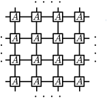
A tensor network is a periodic arrangement of tensors, with links indicating which tensor indices have to be contracted. See Fig. 1 for a tensor network built out of a four-index tensor . We can naturally view such a tensor as a multilinear map:
| (1.1) |
where is a finite-dimensional Euclidean space.
In the tensor network approach, one first rewrites the partition function of a lattice model as a tensor network. This is usually simple to do explicitly, starting from the original lattice Hamiltonian. E.g. in Appendix A we rewrite the 2D Ising model on the square lattice in the form of Fig. 1 using a four-tensor where every index takes only two values, i.e. .
An RG transformation (or map) is a coarse-graining of the tensor network. It rewrites the tensor network in terms of new tensors, fewer in number than the original ones. The simplest rule defines a new tensor by contracting four tensors, as follows:
| (1.2) |
but more sophisticated rules can also be considered (see below). One then iterates this map and studies the resulting RG flow.
We see that is naturally defined on where . It is in fact a general feature of tensor RG maps that they raise the index space dimension. In numerical calculations, reviewed in Appendix C, it is customary to truncate to a subspace of the same dimension as , chosen to minimize the truncation error. In contrast, in this paper we will not use any truncation. Our RG maps will preserve the partition function exactly. Our tensors will be defined in an infinite-dimensional real Hilbert space with a countable basis. For such there exists a (non-unique) isomorphism111I.e. a one-to-one isometric linear map. See also footnote 5. between and . Fixing some such isomorphism , we define the final RG-transformed tensor as
| (1.3) |
Now, tensors and live on the same Hilbert space and can be compared. The RG fixed point equation in this setting reads
| (1.4) |
where is a scalar. Whether this equation has a nontrivial solution may in general depend on the choice of .
It is instructive to compare tensor RG with the more traditional Wilson-Kadanoff RG in terms of Hamiltonians acting on spin variables.222See also [1] for such a comparison and a critical review of tensor RG by Leo Kadanoff and collaborators. There, starting with a lattice Hamiltonian , a new Hamiltonian is defined by the equation:
| (1.5) |
where are the original lattice variables, are the new (block-spin) variables, and is a Kadanoff blocking function required to satisfy the condition for any , which guarantees that the partition function is preserved. The fixed point equation is
In Wilson-Kadanoff RG we have a finite set of possible spin states on each lattice site , replaced in tensor RG by the infinite-dimensional Hilbert space . This is a complication, but it is compensated by two advantages:
-
1.
Tensor RG keeps the interaction short-ranged: only nearest-neighbor tensors are linked by bonds in the network after any number of RG steps. On the contrary, the new Hamiltonian will in general have infinite range after just one Wilson-Kadanoff RG step, even if the original Hamiltonian is short-ranged.
-
2.
The definition of is explicit, unlike that of . In fact, there is no known efficient algorithm to precisely evaluate the couplings of in terms of those of . Some approximate procedures do exist, but they cannot compute the fixed points and their associated critical exponents to very high and systematically improvable accuracy. For the same reason, a rigorous theory of nontrivial Wilson-Kadanoff fixed points has also never been constructed.
These advantages make tensor RG an attractive alternative to the Wilson-Kadanoff scheme. There is a lot of numerical evidence that tensor RG approaches perform very well, at least in 2D (see Appendix C). In this paper we will initiate the rigorous theory of tensor RG.
The rest of the paper is organized as follows. As mentioned, our main goal is to discuss tensor RG near the high-temperature fixed point. This corresponds to the tensor with only one nonzero component . In section 2 we will construct an appropriate RG map and prove that it converges to the high-temperature fixed point super-exponentially fast if we start in a small neighborhood of the fixed point. This is our main result (Theorem 2.1). The RG map will be somewhat more complicated than the basic RG map described above. As we will see, the basic RG map (referred to below as ‘type I’) has eigenvalue 1 for a class of perturbations around in the linearized approximation. To deal with this problem we will introduce another RG map (called ‘type II’). The full RG step will consist of a type I and a type II RG maps applied one after the other.
Convergence to high-temperature fixed point
In this section we will define our RG map and prove that if we start with a tensor sufficiently close to the high-temperature fixed point, then the sequence of tensors we get by iterating this map will converge to the high-temperature fixed point. Our RG map will be a composition of three steps which we will refer to as type 0, type I and type II. The type 0 step is just a gauge transformation, i.e. a change of basis in the Hilbert space . The type I step is the basic RG map described in the introduction. As already mentioned it’s not contractive. Still, we keep it as a part of our RG map because it serves the useful purpose to add some specific structure to our tensor. The type II step, defined below, is the step that integrates out degrees of freedom in such a way that the resulting tensor has a smaller norm difference from than the tensor we started with.
Let us fix a unit vector . The high-temperature fixed point for our RG map will be the tensor in which the only nonzero component is the component and it has value . We denote this tensor by
| (2.1) |
Our tensor will always be a small, real, perturbation of this tensor. We will not have to assume that this perturbation preserves symmetries of the square lattice, i.e. rotations by 90 degrees and reflections (see however Remark 2.1).
As mentioned we will work with infinite-dimensional tensors. Each index will run from 0 to . For tensors with any number of indices we will use the Hilbert-Schmidt norm (also known as the Frobenius norm). For example, if is a 4-index tensor then
| (2.2) |
The number of nonzero components may be finite or infinite, as long as the norm is finite. Finiteness of Hilbert-Schmidt norm is equivalent to the tensor defining a continuous linear mapping from to with . One can think of a tensor abstractly as such a continuous linear mapping, or concretely as an infinite table of real numbers such that the series in the r.h.s. of (2.2) converges.
We will make repeated use of the following property of the Hilbert-Schmidt norm. Let and be tensors of any order. Let be a tensor formed by contracting some of the indices of with indices of . Then the Cauchy-Schwarz inequality implies . This can be iterated, e.g. tensor defined by (2.17) has norm . Also it’s easy to show that the result of such multiple contractions does not depend on the order in which they are performed, if the contracted tensors have finite norm. All these elementary operations on infinite-dimensional Hilbert-Schmidt tensors work exactly as in finite dimension.333For some other operations, such as taking traces or singular value decomposition, finiteness of Hilbert-Schmidt norm may not be enough in infinite dimension. We won’t use those operations in this paper.
Below we will also act on the legs of Hilbert-Schmidt tensors by bounded invertible linear operators. This preserves finiteness of the Hilbert-Schmidt norm. Acting by an isomorphism between and is one example, and other examples (gauge transformations and disentanglers) will be introduced shortly.
We will often represent tensors with a diagram. When a bond is labelled with a , it means that the index on that bond is set to . When it is labelled with an , it means that the index can range over all non-zero indices (if two bonds are labelled with , the indices don’t have to be identical). For unlabelled bonds the index ranges over all values. We think of this diagram as representing the tensor we obtain by setting all components that are not consistent with the bond labelling in the diagram to . The norm of the diagram is then the Hilbert-Schmidt norm of this tensor. For example, the norm of diagram (2.7) is444We make the convention that corresponds to the diagram with on the right, top, left and bottom legs, respectively.
| (2.3) |
When we say that a diagram is we mean that the norm of the tensor associated with the diagram is .
We now introduce three different sets of assumptions A1, A2, A3 on the tensor . Note that A3 is stronger than A2 which is stronger than A1.
-
•
A1:
(2.4) -
•
A2:
![[Uncaptioned image]](/html/2107.11464/assets/x6.png)
(2.5) -
•
A3:
![[Uncaptioned image]](/html/2107.11464/assets/x7.png)
(2.6) In addition, A3 assumes that the only nonzero components of the one-circle tensor are the following “corner” diagram and its rotations:
(2.7) This last assumption includes the assertion that components of the one-circle tensor with only one bond with a nonzero index are zero.
We will prove three propositions. The first will show that if satisfies A1, then a gauge transformation will produce a tensor satisfying A2. The second proposition will show that if satisfies A2, then the type I step will produce a tensor satisfying A3. Finally, the third proposition will show that if satisfies A3, then the type II step will produce a tensor that satisfies A1 with replaced by .
Each of A1, A2, A3 implies that tensor satisfies the normalization condition
| (2.8) |
This condition will in general be disturbed by our tensor manipulations. To restore it, we will normalize the tensor at the end of each RG step, dividing it by a scalar:
| (2.9) |
Type 0
Proposition 2.1.
If satisfies A1, then there is a gauge transformation such that the gauge-transformed satisfies A2, after normalization with .
Proof: A gauge transformation is the insertion of into bonds in the network where is a bounded invertible operator. Since our network is not assumed invariant under rotations by 90 degrees, we will need to use different gauge transformations on the horizontal and vertical bonds, which we denote by and . We will first use to reduce and to and we will then use to do the same for and (recall footnote 4).
Let () be an orthonormal basis of , with as the first element. It is convenient to define a matrix as in the figure:
| (2.10) |
Note that by assumptions. We then let and ( by our conventions for the index). The hypothesis A1 implies that and are . (The norm is the norm.) Define two vectors by
| (2.11) |
We then define the linear operator by
| (2.12) |
Note that . Our gauge transformation for the horizontal bonds will be . So is transformed to :
| (2.13) |
Using the power series expansion of the exponential, we see that
| (2.14) |
We claim that with this choice of we have and both . Let . Then our claim is equivalent to and being both . We have
| (2.15) | |||||
Now let . Since and , the term with these two factors cancels the . We are left with . The norm of this tensor (with a single index ) is since the norm of is and the contributes another since does not appear. Analogously .
Next we apply the gauge transformation on the vertical bonds to . The definition of is completely analogous to the horizontal case. But we need to check that this second gauge transformation does not undo what we accomplished with the first gauge transformation. So we need to show the following diagram is .
| (2.16) |
Note that in this diagram is since it has at least one bond with a nonzero index. Since is of the form , the only term that could be is when both and are replaced by the identity. But this term is because of the first gauge transformation.
The described transformations modify the 0000 component of the tensor making it . E.g. we see that from (2.15). Dividing by we get a tensor satisfying A2, including the normalization condition.
Remark 2.1.
The given proof is valid whether or not preserves lattice symmetries. If is invariant under coordinate reflections, we have , the operator is skew-symmetric and is an orthogonal transformation.
Type I
The type I step is defined by Eqs. (1.2) and (1.3) in the introduction, which we copy here for convenience:
| (2.17) |
| (2.18) |
To fully specify it we must specify an isomorphism . We will assume that is such that:
| (2.19) |
With this condition becomes a fixed point of the type I step. Since an isomorphism preserves the inner product, (2.19) implies that is an isomorphism of the orthogonal complements of and :
| (2.20) |
Clearly, this leaves vastly underdetermined.555We stress however that can be specified very concretely if needed. For the simplest example, arrange the elements of the basis of in a single infinite list in the order of increasing , and of increasing for equal . Then the map mapping to does the job. Proposition 2.2 below is valid for any such .666We could also allow independent maps and on the horizontal and vertical bonds, but we will not need this.
Proposition 2.2 (Type I RG step).
Proof: Assumption A2 decomposes into two tensors. We insert this decomposition of into the definition of and expand to get 16 diagrams. Assumption A3 decomposes into a sum of three tensors, the high-temperature fixed point tensor and two more which we will refer to as the one-circle tensor and the two-circle tensor.
Due to the condition (2.19), the zeroth order term reproduces the high-temperature fixed point tensor, i.e.
| (2.21) |
Here and below, we save space in the diagrams by leaving the contractions with the isomorphism implicit.
We define the one-circle tensor by
| (2.22) |
The notation is shorthand for the additional diagrams that we get by applying reflections about horizontal and vertical lines. Depending on the diagram, these reflections will generate or additional diagrams which we will denote by and , respectively. Recall however that the tensor itself is not required to have any symmetry.
We then define the two-circle tensor to be the sum of the remaining 11 diagrams. Clearly the one-circle tensor is , and the two-circle tensor is . To verify the rest of A3, we note that the only nonzero components of the one-circle tensor are those shown in the two subsequent figures (and rotations thereof):
| (2.23) |
| (2.24) |
where we used hypothesis A2 to estimate the order of diagrams in . Let us move terms in Eq. (2.24) from the one-circle tensor to the two-circle tensor. The A3 assumptions for the one-circle tensor are now satisfied.
At this point the 0000 component of the two circle-tensor is , coming from the diagrams
| (2.25) |
Combining this component with the zero-order term, we can write the tensor as
| (2.26) |
where the one- and two-circle tensors satisfy the assumptions in A3 and is a scalar. It remains to divide by to satisfy A3.
Eigenvalue 1 perturbations
This subsection may be skipped on the first reading as it is not strictly necessary to understand the rest of the construction. It explains a bit better why type I RG map by itself could not achieve our goal, motivating the need to introduce a more complicated type II map.
We see from Proposition 2.2 that the type I RG step maps a tensor with to with . The has some extra structure which will be used in section 2.3. Here we note that since both and are , type I RG map iterates do not converge to superexponentially fast. One may inquire if there is at least exponential convergence, which would mean with some . As we will now show, even this weaker property does not hold. Namely there exist perturbations which are eigenvectors with eigenvalue 1 in the linearized approximation, namely .
For the simplest example of such a perturbation, consider the tensor which has only these four nonzero components, all equal to :
| (2.27) |
To understand better the structure of this tensor, note that it is invariant under parity transformations (flips about horizontal and vertical lines). Consider e.g. flips about horizontal lines. Parity invariance means that the contraction of with 4 vectors remains invariant if we interchange with and simultaneously change , where is a linear operator:
| (2.28) |
Perturbation (2.27) of satisfies this property, as well as the analogous property for flips around vertical lines, for that leaves invariant and exchanges and .
All the components (2.27) are of corner type. Therefore, to linear order in , the correction to tensor is given by the diagram in the top row of Eq. (2.23) and its rotations, namely:
| (2.29) |
The corresponding tensor elements are777The order of tensor components is according to the convention from footnote 4. We also make the convention for numbering basis elements of the tensor product : for vertical bonds the first factor in the tensor product corresponds to the left bond, while for horizontal bonds the first factor corresponds to the top bond.
| (2.30) |
To compute the corresponding we need to complete the definition of the isomorphism, compatibly with (2.20). We define:
| (2.31) |
With this choice of we see that
| (2.32) |
A different choice of would amount to performing an orthogonal gauge transformation, leaving invariant.
So perturbation is left invariant (in the linearized approximation). At the same time, this perturbation can be considered “trivial” in the following sense. If one tries to construct a nonzero contraction of tensor components (2.27) and of the high-temperature tensor, one finds that the lines of indices 1,2 can never form a continuous line traversing the lattice. Rather, such lines “go around” single plaquettes, surrounded by 0 indices, as shown here:
| (2.33) |
Intuitively, this suggests that perturbations of this kind do not introduce long-range correlations in the tensor network. Although type I map fails to filter them, one hopes that a better RG map should be able to do so. Indeed, this will be achieved by type II map introduced below, which will have the property that .
Type II
The type II RG step888This construction was inspired by the TNR algorithm by Evenbly and Vidal [2] from App. C.4. will be a composition of several smaller steps:
-
II.1
Form the tensor by contracting four tensors (same as in type I RG map).
-
II.2
Introduce “disentanglers.” The disentagler is a bounded invertible operator which acts on two indices. We insert into the two horizontal lines between ’s. We then combine with the on its left and the on its right, and call the resulting tensor :
(2.34) This is similar to a gauge transformation except that the procedure operates on two indices. The choice of a good disentangler is a part of defining the RG map, and it will be discussed below.
-
II.3
Represent the tensor as a contraction of two tensors and :
(2.35) -
II.4
Define the tensor by contracting tensors and in the opposite order:
(2.36) Since we are just changing the order of grouping the tensors, contracting ’s gives the same tensor network as before.
- II.5
Proposition 2.3 (type II RG step).
Suppose satisfies A3. There is a choice of the disentangler and of and in II.3 so that the result of the type II RG step satisfies A1 with replaced by , after normalizing with .
Proof: Step II.1 consists in defining as before, Eq. (1.2). Assumption A3 expresses as a sum of three tensors of orders . We insert this sum into each of the four copies of in the definition of and expand this to get diagrams. We denote by the sum of all diagrams which are :
| (2.38) |
Recall that the notations and are shorthand for the additional diagrams that we get by applying reflections about horizontal and vertical lines. We denote by the sum of all the remaining diagrams, which are higher order than . So .
All diagrams in except the last diagram have the property that the indices on the two internal vertical bonds are . We decompose the last diagram as follows:
![[Uncaptioned image]](/html/2107.11464/assets/x29.png) |
(2.39) |
We will refer to the last diagram (with all the bonds labelled) as the dangerous diagram. It is the only diagram in that does not have ’s on both of the vertical bonds. The dangerous diagram is . In labelling its bonds we have made use of the assumption in A3 that the one-circle tensor only has corner nonzero components.
We now proceed to Step II.2 which introduces disentanglers and defines the tensor as in (2.34). We can write , with the understanding that it is the horizontal indices on being contracted in the products as indicated in the figure. The guiding principle to define the disentangler will be to remove the part of the dangerous diagram. We will see below why this is a good idea. The construction will be similar to how in the proof of Proposition 2.1 we constructed gauge transformation removing the part of 000 tensor components.
For and , define and as in the figure:
| (2.40) |
If one or both of and are zero, we define . Then we define
| (2.41) |
where . Note that these two vectors have norm , while in the case of the gauge transformation they had norm . We then define the linear operator from to itself by
| (2.42) |
Note that . We define . So we have
| (2.43) |
where .
We now expand using these expansions and . The key point here is that the two terms cancel the dangerous diagram and its reflection in (2.39). After these cancellations we see that we can write
| (2.44) |
where is the sum of the same diagrams as except the dangerous diagram:
| (2.45) |
while includes
-
•
all diagrams in ;
-
•
all diagrams in except the two terms .
Note that all diagrams in have zero indices on both internal vertical bonds. Note as well that . Achieving these two properties was the main point of the above construction. With and expanded as in (2.43), consists of a finite number of diagrams.
We now pass to step II.3. We will refer to the vertical bond in (2.35) that connects and as the internal -bond. We first define the half-disc tensor when the index on the internal -bond is .
| (2.46) |
We define a similar half-disc by reflecting this figure about a horizontal line. When we contract the two half-discs with the internal -bond restricted to , we get:
| (2.47) |
Note in this contraction the index between the two half-disc is only summed over the single value (the other half-disc tensor components have not yet been defined). The term arises because the contraction in the figure above generates some diagrams that are not in . It’s easy to see that all such diagrams are . We now define
| (2.48) |
We will now show that we can define the rest of the tensor components of these half-disc tensors for indices on the internal -bond other than so that their contraction when the internal -bond ranges over all indices other than reproduces , and so that the full half-discs are . In numerical tensor network RG literature, a typical method of representing a tensor as a contraction of two tensors involves singular value decomposition (SVD). Here we will not use SVD, rather we will use the fact that we know precisely which diagrams appear in . Each such diagram will be naturally written as a contraction of two half-disc tensors (the upper and the lower half of the diagram). Since each diagram is , by moving factors of we will be able to make each of the half-discs .
The Hilbert space for the internal -bond will have the form . is one-dimensional and corresponds to the index for the bond. The rest of the are infinite dimensional (with a countable basis). So this direct sum is isomorphic to the original Hilbert space . Let be the number of diagrams in . For , the contraction of and with the internal -bond restricted to will equal the th diagram in .
We explain how to define and by considering examples of specific diagrams. Recall that we expanded and as in (2.43). We first consider a couple of diagrams in which and have both been replaced by just .
Our first example is:
| (2.49) |
This diagram was in and it enters also in and hence into . It is represented as a contraction of and tensors given by the upper and lower halves of the diagram:
| (2.50) |
The vertical bond space (where is the number of this diagram) is isomorphic to . Note that in this example and , i.e., even smaller than declared above.
For the second example consider the following diagram from :
| (2.51) |
Like in the previous example, we will represent this diagram as a contraction of and tensors given by the upper and lower halves of the diagram. The difference from the previous example is that we need to rescale the tensors by factors to make them both :
| (2.52) |
The vertical bond space is again isomorphic to .999Because of how the high-temperature tensor enters into and , the only nonzero term in the contraction is when both indices on the vertical legs are 0. We could therefore additionally restrict to the one-dimensional space spanned by . This is a minor detail which does not change the scaling of and with .
All the other diagrams in , and the diagrams in where and have both been replaced by just are handled similarly to the above two examples.
For diagrams in which or are not just replaced by , we will need a small lemma representing and as a contraction of two tensors. This will allow us to cut the corresponding diagrams in two.
Lemma 2.1.
1. Tensor can be represented as a contraction of two three-leg tensors
| (2.53) |
where .
2. Tensor in (2.43) can also be represented as a contraction of two three-leg tensors
| (2.54) |
where . Tensor can also be represented in this form, replacing by .
Proof: We denote by and the Hilbert spaces for the vertical bonds joining and tensors in (2.53) and (2.54). We will take to be spanned by two copies of nonzero basis elements of , we index these copies by and where is in . For Part 1, we assign (note a minus sign in the last equation):101010We thank Nikolay Ebel for pointing out a mistake in the previous version of the proof.
| (2.55) |
For Part 2, we note that can be represented in the form (2.54) with
| (2.56) |
and an analogous expression for . It is a direct sum since every term has its own vertical Hilbert space for the term with -tensors. The vertical Hilbert space of the -tensor is the direct sum of Hilbert spaces of individual terms: . The norm of is bounded by .
To represent note that can also be represented as in (2.53) by changing .
We can now consider the remaining diagrams in . They are treated using the same main ideas as in the first two examples: cut the diagram in two and move factors of if needed. Since all the diagrams are , the resulting tensors . We will consider just one example in detail.
Take the following diagram where is replaced by and is replaced by (which we represent as a contraction of and ):
| (2.57) |
We represent it as a contraction of and tensors given by cutting the diagram in two and moving factors:
| (2.58) |
In this case .111111And like in footnote 9 it can be truncated setting the first two indices to 0, without changing the contraction. The other diagrams in which either or is not replaced by are handled similarly.
By moving factors of and using the lemma where needed, we can represent each diagram in as a contraction of two half-disc tensors (the upper and the lower half of the diagram) where the index for the internal -bond ranges over for the th diagram, and each of the half-discs is . Thus we have
| (2.59) |
where the first contraction in the r.h.s. is (2.47) and the second contraction is the representation of , where the index marked with numbers the orthonormal basis of the direct sum . The half-disc tensors are in the first contraction and in the second contraction. This ends step II.3.
Let us now move to step II.4 of our RG map. In it we change how we group terms, defining the tensor as in (2.36). We have:
| (2.60) |
In the second, third and fourth terms one or both contracted tensors are , so those terms are . For the first term we compute the and terms, using the definition (2.46). The term is, after contracting with an isomorphism (step II.5), the high-temperature fixed point tensor. While corrections could in principle arise as cross-terms between piece of and piece of and vice versa, luckily they vanish by the corner structure of the one-circle tensor.121212The part of the tensor is the diagram with a single one-circle tensor insertion in (2.46). Since the one-circle tensor only has corner components, we see that the top indices of this diagram are (or for the reflection). Hence this diagram cannot be contracted with the part of the tensor, which has all indices 0. Nonzero corrections do appear in the next order . In particular the 0000 component becomes . Dividing by it, we get a tensor satisfying A1 with replaced by .
Main result
Theorem 2.1.
Let be a normalized tensor (). It is possible to perform a tensor RG transformation followed by normalization which maps to a normalized tensor with
| (2.61) |
The constant could be extracted by following carefully the proofs of the propositions; we will not do it here. In particular for we have and the iterates of the RG transformations will converge to super-exponentially fast.
Conclusions
In this paper we rigorously formulated a tensor RG approach for the high- phase of 2D lattice models. Of course many other traditional techniques also work in the high- phase, such as the high-temperature expansion. Although at general temperatures the Wilson-Kadanoff RG has not even been defined rigorously, at high one can express it in a rigorous expansion, and show convergence to the high-temperature fixed point [3, 4]. Here we showed how a similar RG stability result can be obtained using tensor RG.
In the future our work can be extended in several directions. In Appendix B we discuss how standard cluster expansions techniques can be used to prove exponential decay of correlation functions when the tensor is close to the high temperature fixed point; we then discuss how the tensor RG might be combined with these expansions to expand the region in which exponential decay can be proven. Another direction for future work is to consider higher-dimensional lattices.
It would be even more interesting to extend tensor RG methods to other situations where traditional RG techniques become complicated. One such situation arises at low temperatures, where the traditional approach has been to apply RG in a contour representation, which introduces some complications [5, 6]. In fact it is known that the Wilson-Kadanoff RG transformation in the spin representation becomes ill-defined at low temperatures (see [7] and [8] for a review).
On the contrary, tensor RG is just as well defined at low as at high temperature. At low and with zero magnetic field, one expects convergence to the low-temperature fixed point described by the direct sum of two high-temperature fixed point tensors. Such convergence is seen in the numerical studies (see Appendix C). It should be possible, and interesting, to establish this rigorously using techniques of the present paper.
Finally, let us discuss the critical temperature. Although Wilson-Kadanoff RG should be well defined at criticality (see [9] for a recent discussion and numerical work), a robust algorithm to evaluate it precisely is lacking. On the contrary, tensor RG evaluation is in principle straightforward. The CDL tensor problem, discussed in Appendix C.2, requires one to complicate tensor RG transformations somewhat compared to the most basic versions, but they remain manageable.
We are therefore optimistic that in the not too distant future the existence of a nontrivial tensor RG fixed point for the 2D Ising and other 2D lattice models will be proved. The proof will proceed in two steps. First, using an appropriate tensor RG transformation, one constructs numerically an approximate RG fixed point. Then, by functional analysis, one proves that an exact fixed point exists nearby. This would therefore be a computer-assisted proof, in the spirit of Lanford’s construction of the Feigenbaum fixed point [10]. We think this is a very interesting open problem.
A similar proof for the critical point of the 3D Ising model would be even more exciting. This should wait until numerical tensor RG methods are able to approximate this fixed point with a good accuracy, which has not yet been achieved (see Appendix C.5).
Acknowledgements
SR is supported by the Simons Foundation grants 488655 and 733758 (Simons Collaboration on the Nonperturbative Bootstrap), and by Mitsubishi Heavy Industries as an ENS-MHI Chair holder.
Data availability statement
Data sharing is not applicable to this article as no datasets were generated or analysed during the current study.
Appendix A Tensor representation for the 2D Ising model
In this appendix we show how to transform the partition function of the nearest-neighbor 2D Ising model on the square lattice with the Hamiltonian , , to a tensor network built out of 4-tensors as in Fig. 1. We present two ways to perform this transformation.
Rotated lattice
This representation was used e.g. in [11]. We start by rotating the spin lattice by 45 degrees. We now associate a tensor with every second square, tensor contractions taking place at the positions of Ising spins:
| (A.1) |
The Hilbert space has two basis elements , . Assigning tensor components
| (A.2) |
we reproduce the 2D Ising model partition function. In finite volume this gives the partition function with periodic boundary conditions on the lattice rotated by 45 degrees.
Transforming the basis to the even () and odd () states
| (A.3) |
the nonzero tensor components become:
| (A.4) |
and rotations thereof. By invariance, they all have an even number of indices.
Unrotated lattice
Alternatively, one can perform the transformation without rotating the lattice [12, 13]. In finite volume, this method gives the partition function with the usual periodic boundary conditions. We start by representing , viewed as a two-tensor in the Hilbert space with basis elements , , as a contraction of two tensors with
| (A.5) |
where , . Graphically
| (A.6) |
Using 0 and 1 to index the columns of the matrix, equations
| (A.7) |
mean that the states 0,1 are, respectively, even and odd. A tensor network representation of the partition function is obtained by defining
| (A.8) |
or graphically
| (A.9) |
The nonzero components are
| (A.10) |
and rotations thereof.
Stability of the high-temperature fixed point
For both representations (A.4) and (A.10), tensor in the limit becomes proportional to the high-temperature fixed point tensor , as component tends to a constant and all others to zero. Theorem 2.1 allows us to conclude that for sufficiently small temperatures the tensor RG iterates of will converge to .
Appendix B Exponential decay of correlators
The results in this paper do not prove exponential decay of correlation functions when the tensor is close to the high temperature fixed point. This is not a shortcoming of the tensor network RG approach compared to the Wilson-Kadanoff RG. For the Wilson-Kadanoff RG one can prove that the RG map is rigorously defined and its iterates converge to the trivial fixed point if the starting Hamiltonian is well inside the high temperature phase [3, 4]. However, this by itself does not imply exponential decay of correlations. Of course, if the Hamiltonian is well inside the high temperature phase then standard high temperature expansion methods can be used to prove exponential decay of correlations. Similarly, standard polymer expansion methods can be used to prove exponential decay of correlations for tensor networks when the tensor is sufficiently close to the high temperature fixed point. We will give a brief sketch of how this is done. This appendix is intended for readers familiar with such techniques, so we will be brief.
We assume that where denotes the high temperature fixed point as before and is small. We use this equation to expand the partition function (the contraction of the tensor network) into a sum of terms where at each vertex in the lattice there is either or . We call a polymer any connected subset of lattice sites. The set of lattice sites with can then be written as the disjoint union of a collection of polymers. The value of this term in the expansion of the partition function is equal to the product of the activities of these polymers where the activity of a polymer is the value of the contraction of the tensor network when there is a at each site in and an at the sites not in . We then have the bound where is the number of vertices in . Then standard polymer expansion methods can be applied if [14]. Here is some small number which will come out from the standard criteria of the polymer expansion convergence.
Where does tensor RG enter this picture? Our Theorem 2.1 proves that if then we can apply tensor RG repeatedly to make arbitrarily small. We have not worked out in this paper what or are. If , then the polymer expansion techniques described above cannot be used directly to show that all these tensor networks are in the high-temperature phase. But combining the two we could do this as follows.
In this paper we discussed tensor RG for the partition function. Correlation function can be represented in terms of a tensor network in which some of the tensors are replaced by other tensors. (The contraction of this network must be divided by the partition function to get the correlation function.) We will refer to these other tensors as tensors. When one applies tensor RG to the network with some tensors, these tensors will be changed as well as the tensors. We do not have any control over how the norm of the tensors may change, but that does not matter. After a finite number of iterations of the RG map the tensor will be sufficienly close to the high temperature fixed point that we can apply a polymer expansion to get exponential decay of the correlation functions.
A calculation of based directly on the proof in this paper may not give a value greater than . Nonetheless we hope that the value of can be improved (i.e., increased) considerably by taking advantage of the fact that the tensor RG map happens locally in space. So there is the possibility that the tensor RG can be used to expand the range of temperatures for which we know that the Ising model (and perturbations of it) are in the high temperature phase.
Appendix C Prior literature on tensor RG131313In this paper the expressions “tensor RG” or “tensor network RG” denote the whole circle of ideas of performing RG using tensor networks, not limited to the TRG and TNR algorithms described in this section.
TRG and its variants
Tensor network approach to RG of statistical physics systems was first discussed in 2006 by Levin and Nave [15]. The precise method they introduced, called Tensor RG (TRG), consists in representing tensor as the product , graphically
| (C.1) |
and then defining a new tensor by contracting four tensors:
| (C.2) |
Decomposition (C.1) is obtained from the singular value decomposition (SVD) with diagonal and . To keep the bond dimension finite, the singular value decomposition is truncated to the largest singular values out of the total of . Ref. [15] also defined a similar procedure for the honeycomb lattice. TRG can be used to evaluate numerically the free energy of the 2D Ising model as a function of the temperature and of the external magnetic field on a large finite lattice (reducing it to a one-site lattice by a finite number of TRG steps), and then extract the infinite volume limit by extrapolation. Using bond dimensions up to , Ref. [15] attained excellent agreement with the exact result except in a small neighborhood of the critical point.
In the introduction we mentioned a simple tensor network RG based on Eq. (1.2), which was also the basis for type I RG step in section 2.2. This procedure was first carried out in [12],141414For illustrative purposes, Eq. (1.2) also appeared in [11]. called there HOTRG since it used higher-order SVD in the bond dimension truncation step. More precisely, HOTRG first contracts tensors pairwise in the horizontal direction, and then pairwise in the vertical direction. HOTRG agrees with the exact 2D Ising free energy even better than TRG. Applied to the 3D Ising, it gives results in good agreement with Monte Carlo. The accuracy of TRG and HOTRG is further improved by taking into account the effect of the “environment” to determine the optimal truncation, in methods called SRG [16, 17] and HOSRG [12].
CDL tensor problem
Although TRG and its variants performed very well in numerical free energy computations, it was noticed soon after its inception [18] that the method has a problem. There is a class of tensors describing lattice models with degrees of freedom with ultra-short-range correlators only, which are not coarse-grained away by the TRG method and its above-mentioned variants but passed on to the next RG step unchanged, being exact fixed points of the TRG transformation. These “corner double line” (CDL) tensors (named so in [11]) have a bond space with two indices and the components
| (C.3) |
or graphically
| (C.4) |
with arbitrary matrices . CDL tensors present a problem both conceptually and practically:
-
•
Conceptually, as we would like to describe every phase by a single fixed point, not by a class of equivalent fixed points differing by a CDL tensor.
-
•
Practically, since every numerical tensor RG computation is performed in a space of finite bond dimension, limited by computational resources. It is a pity to waste a part of this space on uninteresting short-range correlations described by the CDL tensors. This becomes especially acute close to the critical point.
We proceed to discuss algorithms trying to address this problem.
TEFR
TEFR (tensor entanglement filtering renormalization) was the first algorithm aiming to resolve the problem of CDL tensors [11]. It consists of the following steps:
-
1.
Perform SVD to represent as in Eq. (C.1), truncating to the largest singular values so that the representation is approximate, where is the original bond dimension. Tensor thus has dimension .151515Two three-tensors appearing in the decomposition (C.1) may in general be different but we will treat them here as identical for simplicity. The same comment applies to tensors and below.
-
2.
Find a tensor of dimension with so that161616More generally, the four tensors marked by don’t have to be identical, but we will assume that they are identical to simplify the notation.
(C.5) where dashed bonds have dimension .
-
3.
Recombine tensors to form a four-tensor with dimension :
(C.6) -
4.
Perform an SVD to represent along the “other diagonal”:
(C.7) -
5.
Contract tensors to form tensor , the final result of the RG step:
(C.8)
The rationale behind this algorithm is that it reduces an arbitrarily large CDL tensor to a tensor of dimension one in a single RG step [11]. It is less clear what happens for tensors which are not exactly CDL. Ref. [11] gives several procedures for how to perform the key Step 2 for such tensors, but it’s not clear if these are fully successful. Numerical results of [11] for the 2D Ising model are inconclusive. TEFR RG flow converges to the high-temperature fixed point tensor for , to the low-temperature fixed point tensor for , while in the intermediate range around it converged to a -dependent tensor with many nonzero components.
Gilt-TNR algorithm (App. C.5 below) improves on TEFR by providing a more robust procedure for Step 2.
TNR
TNR (tensor network renormalization) algorithm by Evenbly and Vidal [2] was perhaps the first method able to address efficiently the CDL tensor problem. It gives excellent results when applied to the 2D Ising model [2], including the critical point. It runs as follows:171717We present the algorithm rotated by 90 degrees compared to [2].
-
1.
Choose a unitary transformation of (“disentangler”). Inserting into the tensor network does not change its value:
(C.9) -
2.
Choose a couple of isometries . Optimize , , so that
(C.10) -
3.
Rearrange the tensor network as
(C.11) where (each blue triangle stands for one of the , tensors)
(C.12) -
4.
Perform an (approximate because truncated) SVD for the and tensors:
(C.13) -
5.
Finally define the end result of the RG step as
(C.14)
Our type II RG step (section 2.3) was inspired by the TNR algorithm. The main differences and similarities are as follows:
-
•
We work in an infinite-dimensional Hilbert space.
-
•
Our disentanglers don’t have to be unitary. We insert instead of .
-
•
We do not choose and to minimize the error in (C.10). Rather, our , are the identity on , while is chosen to “disentangle” certain correlations between the upper and lower part of TNR (whose section 2.3 analogue is called ), by killing the part of the “dangerous diagram” in (2.39). Since our ’s are the identity, our is simply a product of Kronecker deltas, realizing a contraction among the indices of tensors
- •
- •
Further algorithms aiming to resolve the CDL problem include Loop-TNR [19] and TNR+ [20].
Gilt-TNR
Gilt(graph independent local truncation)-TNR [13] follows the same steps as TEFR from Appendix C.3. It improves on TEFR by providing a very efficient way to perform Step 2, reducing dimensions of the contraction bonds in the l.h.s. of (C.5) one bond at a time. See [13] for details.
Gilt-TNR is perhaps the simplest tensor network algorithm able to deal with the CDL problem. In addition to the usual 2D Ising benchmarking, Ref. [13] showed some preliminary results concerning its performance in 3D. It would be interesting to see a computation of the 3D Ising critical exponents by this or any other tensor RG method.
References
- [1] E. Efrati, Z. Wang, A. Kolan, and L. P. Kadanoff, “Real-space renormalization in statistical mechanics,” Rev. Mod. Phys. 86 no. 2, (2014) 647–667, arXiv:1301.6323 [cond-mat.stat-mech].
- [2] G. Evenbly and G. Vidal, “Tensor Network Renormalization,” Phys. Rev. Lett. 115 no. 18, (2015) 180405, arXiv:1412.0732 [cond-mat.str-el].
- [3] R. B. Griffiths and P. A. Pearce, “Mathematical properties of position-space renormalization-group transformations,” J. of Stat. Phys. 20 no. 5, (1979) 499–545.
- [4] I. A. Kashapov, “Justification of the renormalization-group method,” Theor. and Math. Phys. 42 no. 2, (1980) 184–186.
- [5] K. Gawedzki, R. Kotecký, and A. Kupiainen, “Coarse-graining approach to first-order phase transitions,” J. Stat. Phys. 47 no. 5, (1987) 701–724.
- [6] J. Bricmont and A. Kupiainen, “Phase transition in the 3d random field Ising model,” Comm. Math. Phys. 116 no. 4, (1988) 539–572.
- [7] A. C. D. van Enter, R. Fernández, and A. D. Sokal, “Regularity properties and pathologies of position-space renormalization-group transformations: Scope and limitations of Gibbsian theory,” J. Stat. Phys. 72 no. 5-6, (1993) 879–1167.
- [8] J. Bricmont, A. Kupiainen, and R. Lefevere, “Renormalizing the renormalization group pathologies,” Phys. Rep. 348 no. 1, (2001) 5–31.
- [9] T. Kennedy, “Renormalization Group Maps for Ising Models in Lattice-Gas Variables,” J. Stat. Phys. 140 no. 3, (2010) 409–426, arXiv:0905.2601 [math-ph].
- [10] O. E. Lanford, “A computer-assisted proof of the Feigenbaum conjectures,” Bull. Amer. Math. Soc. (N.S.) 6 no. 3, (1982) 427–434. https://projecteuclid.org:443/euclid.bams/1183548786.
- [11] Z.-C. Gu and X.-G. Wen, “Tensor-entanglement-filtering renormalization approach and symmetry-protected topological order,” Phys. Rev. B 80 no. 15, (2009) 155131, arXiv:0903.1069 [cond-mat.str-el].
- [12] Z. Y. Xie, J. Chen, M. P. Qin, J. W. Zhu, L. P. Yang, and T. Xiang, “Coarse-graining renormalization by higher-order singular value decomposition,” Phys. Rev. B 86 no. 4, (2012) 045139, arXiv:1201.1144 [cond-mat.stat-mech].
- [13] M. Hauru, C. Delcamp, and S. Mizera, “Renormalization of tensor networks using graph independent local truncations,” Phys. Rev. B 97 no. 4, (2018) 045111, arXiv:1709.07460 [cond-mat.str-el].
- [14] R. Kotecký and D. Preiss, “Cluster expansion for abstract polymer models,” Commun. Math. Phys. no. 103, (1986) 491–498.
- [15] M. Levin and C. P. Nave, “Tensor renormalization group approach to 2D classical lattice models,” Phys. Rev. Lett. 99 no. 12, (2007) 120601, arXiv:cond-mat/0611687.
- [16] Z. Y. Xie, H. C. Jiang, Q. N. Chen, Z. Y. Weng, and T. Xiang, “Second Renormalization of Tensor-Network States,” Phys. Rev. Lett. 103 no. 16, (2009) 160601, arXiv:0809.0182 [cond-mat.str-el].
- [17] H. H. Zhao, Z. Y. Xie, Q. N. Chen, Z. C. Wei, J. W. Cai, and T. Xiang, “Renormalization of tensor-network states,” Phys. Rev. B 81 no. 17, (2010) 174411, arXiv:1002.1405 [cond-mat.str-el].
- [18] M. Levin, “Real space renormalization group and the emergence of topological order,”. talk at the workshop ‘Topological Quantum Computing’, Institute for Pure and Applied Mathematics, UCLA, February 26-March 2, 2007.
- [19] S. Yang, Z.-C. Gu, and X.-G. Wen, “Loop optimization for tensor network renormalization,” Phys. Rev. Lett. 118 no. 11, (2017) , arXiv:1512.04938 [cond-mat.str-el].
- [20] M. Bal, M. Mariën, J. Haegeman, and F. Verstraete, “Renormalization group flows of Hamiltonians using tensor networks,” Phys. Rev. Lett. 118 (2017) 250602, arXiv:1703.00365 [cond-mat.stat-mech].
- [21] X. Lyu, R. G. Xu, and N. Kawashima, “Scaling dimensions from linearized tensor renormalization group transformations,” Phys. Rev. Res. 3 no. 2, (2021) 023048, arXiv:2102.08136 [cond-mat.stat-mech].