Thermalization of Gauge Theories from their Entanglement Spectrum

Abstract

Using dual theories embedded into a larger unphysical Hilbert space along entanglement cuts, we study the Entanglement Structure of $\mathbf{Z}_{2}$ lattice gauge theory in $(2+1)$ spacetime dimensions. We demonstrate Li and Haldane’s conjecture, and show consistency of the Entanglement Hamiltonian with the Bisognano-Wichmann theorem. Studying non-equilibrium dynamics after a quench, we provide an extensive description of thermalization in $\mathbf{Z}_{2}$ gauge theory which proceeds in a characteristic sequence: Maximization of the Schmidt rank and spreading of level repulsion at early times, self-similar evolution with scaling coefficients $\alpha=0.8\pm 0.2$ and $\beta=0.0\pm 0.1$ at intermediate times, and finally thermal saturation of the von Neumann entropy.

Introduction. Understanding thermalization of isolated quantum systems is an outstanding challenge in many fields, from atomic gases at ultra-cold temperatures [1, 2, 3], condensed matter physics [4, 5, 6, 7], cosmology [8], to high energy and nuclear physics [9, 10, 11, 12, 13, 14]. Much progress has been made in various systems based on the Eigenstate Thermalization Hypothesis (ETH) [15, 16, 17], but not much is known for gauge theories, i.e. systems with an extensive number of local constraints.

Entanglement structure, more precisely the Entanglement Spectrum (ES), first suggested by Li and Haldane as an indicator of topological order (TO) in fractional quantum hall effect states [18], has recently become the subject of multiple such studies [19, 20, 21, 22, 23, 24, 25, 26, 27]. Their extension to lattice gauge theories (LGTs) is ambiguous because gauge invariance allows no local tensor product structure of the physical Hilbert space (HS). This issue has been addressed in recent years [28, 29, 30, 31, 32, 33, 34].

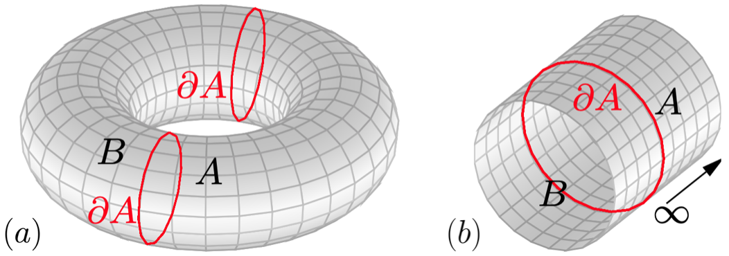
Figure 1: Lattices with entanglement cuts considered in this work. (a) Torus and (b) infinite cylinder with entanglement boundary/boundaries $\partial A$.

In this letter, we use dual theories [35, 36, 37] of $\mathbf{Z}_{2}$ LGT in (2+1) spacetime dimensions ($\mathbf{Z}_{2}^{2+1}$) embedded into a larger unphysical HS only along ‘entanglement’ cuts, allowing access to the ES by naively ‘taking the trace’. With this, we demonstrate Li and Haldane’s entanglement-boundary conjecture for $\mathbf{Z}_{2}^{2+1}$ in the TO phase [18], analytically on an infinite half-cylinder using perturbation theory and numerically on a finite torus at arbitrary coupling. A variational approach [38] allows us to reconstruct the Entanglement Hamiltonian (EH) of ground states, consistent with expectations from the Bisognano-Wichmann (BW) theorem [39, 40].

Our main effort is devoted to probing thermalization of LGTs through the ES. Focussing on out-of-equilibrium dynamics after quenches with initial states in the TO, as well as the trivial (confined) phase of the model, we track the evolution of the symmetry resolved ES [41, 42, 43, 44, 45, 46, 47]: At early times the Schmidt rank is maximized, followed by spreading of level repulsion through the ES, and saturation of the entanglement entropy at parametrically later times. Remarkably, in an intermediate stage the approach to equilibrium is characterized by self-similarity of the ES, reminiscent of classical wave turbulence and universal behavior [48, 49, 50, 51].

Despite being restricted to small systems, our ES analysis is remarkably robust and provides a promising path towards understanding the thermalization of Abelian and non-Abelian gauge theories, e.g. in Quantum Chromodynamics (QCD) [14]. Our approach is suited for exploration with tensor networks [52, 53, 54] in the case of ground and low energy states, as well as near-future digital quantum computers and analog quantum simulators [55, 56, 57, 58, 59, 60, 61, 62, 63, 64, 65, 66] (see e.g. [67, 68, 69] for $\mathbf{Z}_{2}$ LGT).

Entanglement Structure of $Z_{2}$ Gauge Theory. We consider $\mathbf{Z}_{2}^{2+1}$ LGT with Hamiltonian

$$H=-\sum_{\mathbf{n}}\sigma^{z}_{\mathbf{n},x}\sigma^{z}_{\mathbf{n}+\hat{x},y}\sigma^{z}_{\mathbf{n}+\hat{y},x}\sigma^{z}_{\mathbf{n},y}-\epsilon\sum_{\mathbf{n},i=x,y}\sigma^{x}_{\mathbf{n},i}\,,$$ (1)

with $\mathbf{n}=(n_{x},n_{y})$, $n_{i}\in[0,N_{i}-1]$ and $i=x,y$ where $\sigma^{z}_{\mathbf{n},i}$ ($\sigma^{x}_{\mathbf{n},i}$) are Pauli operators positioned on the links of a two-dimensional rectangular lattice with $N_{x}\times N_{y}$ sites. Gauge invariance is expressed as $[H,G_{\mathbf{n}}]=0$ with $G_{\mathbf{n}}=\sigma^{x}_{\mathbf{n},x}\sigma^{x}_{\mathbf{n}-\hat{x},x}\sigma^{x}_{\mathbf{n},y}\sigma^{x}_{\mathbf{n}-\hat{x},y}\,$ and Gauss law defines the physical subspace as $G_{\mathbf{n}}|\psi^{\rm phys}\rangle=|\psi^{\rm phys}\rangle$.

$\mathbf{Z}_{2}^{2+1}$ LGT has two ground state phases: a topologically trivial phase (confined), as well as a phase with topological order (TO). In the TO phase, for $\epsilon<\epsilon_{c}$, the ground state manifold is fourfold degenerate (on a torus), labelled by eigenvalues of ‘ribbon’ operators $V_{x}\equiv\prod_{\mathbf{n}\in\mathcal{C}_{x}}\sigma^{x}_{\mathbf{n},i}$ and $V_{y}\equiv\prod_{\mathbf{n}\in\mathcal{C}_{y}}\sigma^{x}_{\mathbf{n},i}$, winding around the $x$- and $y$-directions, with $[V_{x},H]=[V_{y},H]=0$ .

In the following, we consider the entanglement properties of a bipartition $N_{x}\equiv N_{x}^{A}+N_{x}^{B}$ of a torus, see Fig. 1(a). Before considering thermalization dynamics, we first validate our approach of computing LGT Entanglement Structure by demonstrating Li and Haldane’s conjecture [18]: TO is manifest in the entanglement structure of states; the low lying part of the ES is equal (up to rescaling) to the physical spectrum of boundary excitations at the entanglement cut.

The basis of our analysis are dual formulations of Eq. (1) embedded into a larger, unphysical HS along boundaries: (a) for the torus with aforementioned entanglement bipartition [Fig. 1(a)], as well as (b) an infinite (half) cylinder with physical boundaries [Fig. 1(b)], see Supplemental Material. Our dual approach is a generalization of that of Wegner [35], and unlike the latter where all Gauss laws are eliminated, it captures the entanglement structure stemming from the Gauss laws between the two subsystems, as we demonstrate below by verifying Li and Haldane’s conjecture. By also resulting in a smaller Hilbert space, it reduces the numerical cost significantly compared to a direct implementation of Eq. (1).

To demonstrate Li and Haldane’s conjecture, we consider first the semi-infinite cylinder A with physical ‘open electric’ boundary conditions $\partial A$ in Fig. 1(b) [37, 33]. The corresponding dual Hamiltonian reads

$$H_{A}= -\sum_{\mathbf{n},n_{x}>0}\mu^{z}_{\mathbf{n}}-\sum_{\mathbf{n},n_{x}=0}\mu^{z}_{\mathbf{n}}\sigma^{z}_{\mathbf{n},y}$$

$$-\epsilon\sum_{\mathbf{n},n_{x}>0}\mu^{x}_{\mathbf{n}}\mu^{x}_{\mathbf{n}-\hat{x}}-\epsilon\sum_{\mathbf{n},n_{x}=0}\sigma^{x}_{\mathbf{n},y}$$

$$-\epsilon\sum_{\mathbf{n},n_{y}>0}\mu^{x}_{\mathbf{n}}\mu^{x}_{\mathbf{n}-\hat{y}}-\epsilon\sum_{\mathbf{n},n_{y}=0}\mu^{x}_{\mathbf{n}}\mu^{x}_{\mathbf{n}-\hat{y}}V_{y}$$

$$-\epsilon\sum_{n_{y}=1}^{N_{y}-1}\sigma^{x}_{{\scriptscriptstyle(-1,n_{y})},x}\,.$$ (2)

This contains two sets of Pauli operators: dual gauge invariant operators $\mu^{x/z}_{\mathbf{n}}$ in the bulk as well as the original gauge-variant variables $\sigma^{x/z}_{\mathbf{n},i}$ on $\partial A$. Here, $\sigma^{x}_{{\scriptscriptstyle(-1,n_{y})},x}$ is the electric flux through the boundary, see also Supplemental Material. While gauge-redundancy is eliminated in the bulk, Gauss law on $\partial A$ is not eliminated, $G_{n_{y}}\equiv\sigma^{x}_{{\scriptscriptstyle(-1,n_{y})},x}\sigma^{x}_{{\scriptscriptstyle(0,n_{y})},y}\sigma^{x}_{{\scriptscriptstyle(0,n_{y}-1)},y}\mu^{x}_{\mathbf{n}}\mu^{x}_{\mathbf{n}-\hat{y}}$ (for $n_{y}>0$) and $\sigma^{x}_{{\scriptscriptstyle(-1,n_{y})},x}\sigma^{x}_{{\scriptscriptstyle(0,n_{y})},y}\sigma^{x}_{{\scriptscriptstyle(0,n_{y}-1)},y}\mu^{x}_{\mathbf{n}}\mu^{x}_{\mathbf{n}-\hat{y}}V_{y}$ (for $n_{y}=0$).

To demonstrate Li and Haldane’s conjecture, we first compute the boundary theory. The ground state for $\epsilon=0$, $V_{y}=1$ is given by $|\Omega^{A}\rangle=P_{G}|\mathord{\uparrow}\rangle$ where $|\mathord{\uparrow}\rangle$ is the state with plaquette eigenvalue $1$, i.e. $\mu^{z}_{\mathbf{n}}|\mathord{\uparrow}\rangle=|\mathord{\uparrow}\rangle$ in the bulk ($n_{x}>0$) and $\mu^{z}_{\mathbf{n}}\sigma^{z}_{\mathbf{n},y}|\mathord{\uparrow}\rangle=|\mathord{\uparrow}\rangle$ on $\partial A$ ($n_{x}=0$); $P_{G}\equiv\prod_{n_{y}}(1+G_{n_{y}})/2$ is a projector onto the physical subspace. We compute the ground state for small $\epsilon$ perturbatively [71] (see [72, 73, 74, 34] for the opposite limit), resulting in a low energy effective Hamiltonian $H_{A}^{\rm eff}$ describing excitations on $\partial A$, see Supplemental Material,

$$H_{A}^{\rm eff}=-\epsilon\sum_{n_{y}=0}^{N_{y}-1}\sigma^{x}_{{\scriptscriptstyle(0,n_{y})},y}\sigma^{x}_{{\scriptscriptstyle(0,n_{y}-1)},y}\;\mu^{x}_{{\mathbf{n}}}\;\mu^{x}_{{\mathbf{n}-\hat{y}}}+O(\epsilon^{2})\,.$$ (3)

Here, we omitted the projector onto $|\mathord{\uparrow}\rangle$, given by $\prod_{\mathbf{n}}(1+W_{\mathbf{n}})/2$ with $W_{\mathbf{n}}=\mu^{z}_{\mathbf{n}}\sigma^{z}_{{\scriptscriptstyle(0,n_{y})},y}$ ($n_{x}=0$) and $W_{\mathbf{n}}=\mu^{z}_{\mathbf{n}}$ ($n_{x}>0$), and constant terms.

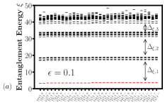
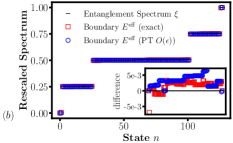
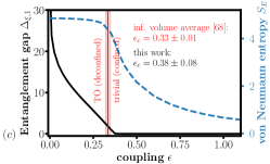
Figure 2: (a) Entanglement Spectrum $\xi_{n}$ of the groundstate for $\epsilon=0.1$ and $(N_{x}^{A}+N_{x}^{B})\times N_{y}=(3+3)\times 3$, corresponding to the entanglement cut in Fig. 1(a), resolved into symmetry sectors. (b) Rescaled low energy part of the entanglement spectrum for $\epsilon=0.1$, and $(N_{x}^{A}+N_{x}^{B})\times N_{y}=(3+3)\times 4$, versus the spectrum of $H_{A}^{\rm eff}$: numerical (exact diagonalization) and analytical (perturbation theory). (c) Entanglement gap $\Delta_{\xi,1}$ between low and high energy parts of ES (black), and von-Neumann Entropy (blue) as a function of coupling $\epsilon$ for $(N_{x}^{A}+N_{x}^{B})\times N_{y}=(3+3)\times 4$ versus infinite volume average $\epsilon_{c}$ from table II of [75].

We now compute the ES for $\partial A$ a (virtual) entanglement cut of the infinite cylinder $A+B$, see Fig. 1(b). The density matrix of the ground state is [at $O(\epsilon)$]

$$\rho_{{A+B}}= \Bigg{(}\frac{1}{2}-\frac{\epsilon}{4}\Big{[}\sum_{\begin{subarray}{c}\mathbf{n},i\\ \not\in\partial A\end{subarray}}\mu^{x}_{{\mathbf{n}}}\mu^{x}_{{\mathbf{n}-\hat{i}}}+\sum_{{n_{y}=0}}^{{N_{y}-1}}\sigma^{x}_{{\scriptscriptstyle(0,n_{y})},\scriptscriptstyle{y}}\Big{]}\Bigg{)}\rho^{(0)}+\rm{h.c.}\,,$$ (4)

with $\rho^{(0)}\equiv\prod_{n_{y}}(1+G_{n_{y}})/2\,\prod_{\mathbf{n}}(1+W_{\mathbf{n}})/2$, where $W_{\mathbf{n}}=\mu^{z}_{\mathbf{n}}\sigma^{z}_{{\scriptscriptstyle(0,n_{y})},y}$ for $n_{x}\in\{0,-1\}$ and $W_{\mathbf{n}}=\mu^{z}_{\mathbf{n}}$ for $n_{x}<-1$ and $n_{x}>0$. In Eq. (4), _{n,i／∈∂A} indicates summation over links in $A+B$ away from the entanglement cut. The reduced density matrix of system $A$ follows as

$${\rho}_{A}=\Bigg{(}\frac{1}{2}-\frac{\epsilon}{4}\Big{[}\sum_{\begin{subarray}{c}\mathbf{n},i\in A\\ \not\in\partial A\end{subarray}}\mu^{x}_{\mathbf{n}}\mu^{x}_{\mathbf{n}-\hat{i}}+\sum_{n_{y}=0}^{N_{y}-1}\sigma^{x}_{{\scriptscriptstyle(0,n_{y})},y}\,$$

$$-\sum_{n_{y}=0}^{N_{y}-1}\mu^{x}_{{\scriptscriptstyle(0,n_{y})}}\mu^{x}_{{\scriptscriptstyle(0,n_{y}-1)}}\sigma^{x}_{{\scriptscriptstyle(0,n_{y})},y}\sigma^{x}_{{\scriptscriptstyle(0,n_{y}-1)},y}\Big{]}\,\Bigg{)}\rho^{(0)}_{A}+{\rm h.c.},$$ (5)

with $\rho^{(0)}_{A}\equiv\mathbb{I}^{\partial A}/2^{N_{y}}\prod_{\mathbf{n}\in A}(1+W_{\mathbf{n}})/2$ and $\mathbb{I}^{\partial A}$ a $2^{N_{y}}$ dimensional unit matrix on $\partial A$. We thus obtain the EH $H_{A}^{\rm ent}=-\log(\rho_{A})$ from Eq. (Thermalization of Gauge Theories from their Entanglement Spectrum),

$$H_{A}^{\rm ent}=N_{y}\log(2)+\frac{\epsilon}{2}\sum_{n_{y}=0}^{N_{y}-1}\sigma^{x}_{{\scriptscriptstyle(0,n_{y})},y}\sigma^{x}_{{\scriptscriptstyle(0,n_{y}-1)},y}\;\mu^{x}_{{\mathbf{n}}}\;\mu^{x}_{{\mathbf{n}-\hat{y}}}\,,$$ (6)

omitting again the projector $\prod_{\mathbf{n}\in A}(1+W_{\mathbf{n}})/2$. Eq. (6) has precisely the same form as Eq. (3), $H_{A}^{\rm ent}\simeq H_{A}^{\rm eff}$, demonstrating (perturbatively) Li and Haldane’s conjecture for $\mathbf{Z}^{2+1}_{2}$ lattice gauge theory.

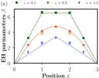
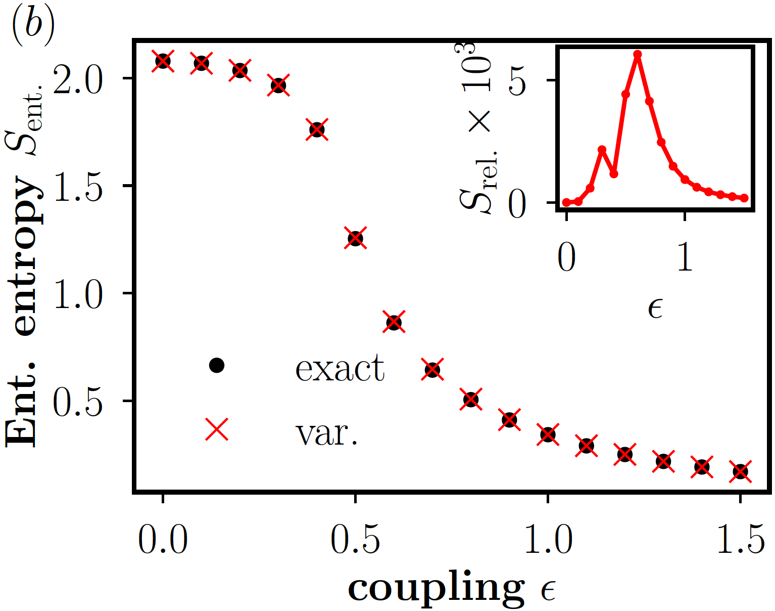
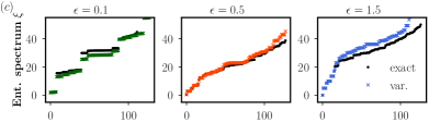
Figure 3: (a) Optimal EH parameters for the local approximation $\sigma_{A}$. Thick markers and light crosses correspond to electric and magnetic energy contributions, respectively. The dotted, orange line is a parabolic fit; the other dotted, green and blue lines are guides for the eye. (b) Exact (black dots) and optimal variational (red crosses) entanglement entropy. Inset: relative entropy. $(c)$ Exact (black dots) and optimal variational (colored crosses) ES for the same values of $\epsilon$ shown in (a). All data are obtained for a (sub)system of size $(N_{x}^{A}+N_{x}^{B})\times N_{y}=(3+3)\times 2$.

To probe the validity of this equivalence beyond perturbation theory, we turn to numerical simulations with exact diagonalization [76]. We consider a torus separated by two entanglement cuts into systems $A+B$, shown in Fig. 1(a). The ES $\xi_{n}$ of states $n=1,\dots,{\rm{\dim}}(\rho_{A})$ in $A$ is shown in Fig. 2(a), separated into symmetry sectors, specified by the electric flux operators into the system on both boundaries ($\mathord{\uparrow}/\mathord{\downarrow}$) and a string of electric field operators  $\tilde{V}_{x}=\prod_{\mathbf{n}\in\tilde{\mathcal{C}}}\sigma^{x}_{\mathbf{n},i}$ across a path $\tilde{\mathcal{C}}$ from one boundary to the other ($\pm$), see Supplemental Material. Fig. 2(b) shows the smallest eigenvalues (‘low energy part’) of the ES compared to the boundary spectrum of $H_{A}$ for $\epsilon=0.1$, displaying near perfect agreement with each other and with our perturbative result. This agreement holds in the TO phase with good precision up to finite size corrections.

Another signature of TO are Entanglement Gaps of the ES $\Delta_{\xi,{i}}$ shown in Fig. 2(a) and (c), the latter displaying $\Delta_{\xi,{1}}$ as a function of $\epsilon$. Defining the TO/confinement phase transition $\epsilon_{c}$ at $\Delta_{\xi,{1}}\rightarrow 0$ results in $\epsilon_{c}=0.38\pm 0.09$ agreeing within errorbars with the infinite volume result $\epsilon_{c}=0.33\pm 0.01$ [75], see Supplemental Material where we demonstrate robustness against finite-volume effects.

The Bisognano-Wichmann (BW) theorem, and its extensions [39, 40], captures another aspect of the EH; it states that the EH of the ground state is a local deformation of the system Hamiltonian. Using an ansatz to approximate the reduced density matrix $\rho_{A}\approx\sigma_{A}\propto\exp\left(-\sum_{\mathbf{n}\in A}\beta_{\mathbf{n}}h_{\mathbf{n}}\right)$, with $h_{\mathbf{n}}$ denoting gauge-invariant local operators in $A$, we test its applicability to LGTs. Optimal local parameters $\beta_{\mathbf{n}}$, obtained by minimizing the relative entropy $S(\rho_{A}||\sigma_{A})$, are shown in Fig. 3(a), see also Supplemental Material.

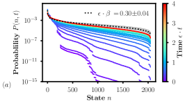
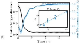
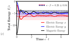
Figure 4: (a) ES as a function of time ($(N_{x}^{A}+N_{x}^{B})\times N_{y}=(3+5)\times 3$) versus that of a thermal system (black dotted line). (b) Von Neumann entropy and Bhattacharyya distance to a thermal system. Inset: Dependence of the saturated entropy on the volume $V_{A}$ of $A$. (c) Electric and magnetic energy compared to thermal expectation values ($N_{x}\times Ny=(3+3)\times 3$). In (a) $\beta$ is determined from the saturated entanglement entropy in (b), while in (c) it is determined from the energy density of the initial state. Bands and error bars indicate uncertainties due to finite-size effects, determined from the difference between largest and second-largest lattices.

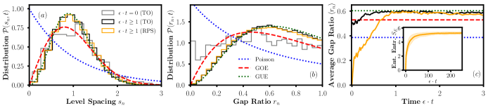
Figure 5: (a) Distribution $\mathcal{P}(s_{n})$ of level spacings (of the unfolded ES), for the quench from $\epsilon=0.1\rightarrow 1$ (gray and black curves) versus $\epsilon\rightarrow\infty$ (confined phase) as initial condition (orange curve). (b) Gap ratio distribution $\mathcal{P}(r_{n})$. (c) Average gap ratio $\langle r_{n}\rangle$ as a function of time. Inset: Growth of von Neumann entropy for the quench $\epsilon=\infty\rightarrow 1$. (Shown for $(N_{x}^{A}+N_{x}^{B})\times(3+5)\times 3$ lattice sites.)

Our results are consistent with a parabolic deformation in the vicinity of the phase transition, as expected from BW for a conformal field theory. While the deformation deviates from a parabola away from the critical point, the overall quality of the approximation $H^{\text{ent}}_{A}\approx-\log\sigma_{A}$ is excellent, see Fig. 3(b) and Fig. 3(c), comparing the exact ES to its variational approximation. The local deformation captures the low energy part of the ES almost perfectly for all $\epsilon$, except for small deviations at high energy which do not contribute significantly to the entanglement entropy.

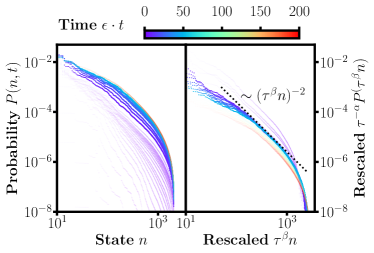
Figure 6: Left: Un-rescaled Schmidt spectrum $P(n,t)=\exp\{-\xi_{n}\}$ for the quench $\epsilon=\infty\rightarrow 1$ at different times. Right: Rescaled Spectrum. The approach to thermalization is characterized by a self-similar universal form $P(n,t)=\tau^{-\alpha}P(\tau^{\beta}n)$, $\tau\equiv\epsilon(t-t_{0})$ for times $2\lessapprox\epsilon\cdot t\lessapprox 60-100$. A black dotted line indicates power law behavior $(\tau^{\beta}n)^{-2}$. The spectrum outside the scaling window is shaded out. (Shown for $(N_{x}^{A}+N_{x}^{B})\times(3+5)\times 3$ lattice sites.)

Thermalization from the Entanglement Spectrum. To characterize thermalization dynamics, we extract the ES of non-equilibrium states in the following. We prepare a (randomly chosen) excited eigenstate of $H(\epsilon=0.1)$ as initial state and evolve with $H(\epsilon=1)$. Fig. 4(a) demonstrates thermalization, showing the corresponding Schmidt spectrum $P(n,t)\equiv\exp\{-\xi_{n}(t)\}$ of subsystem $A$ [$N_{x}\times N_{y}=(3+5)\times 3$] approaching the thermal limit (black dotted line) at late times. Thermalization occurs when expectation values are equal to those derived from a canonical ensemble, i.e. $\rho^{\rm therm.}_{A}=\text{Tr}_{B}(\rho^{\rm can.})/\text{Tr}(\rho^{\rm can.})$ where $\rho^{\rm can.}=\exp\{-\beta H\}$ [77]. In Fig. 4(a), we use an approximate, but numerically simpler, form $\rho_{A}^{\rm therm.}\approx e^{-\beta H_{A}}/\text{Tr}_{A}(e^{-\beta H_{A}})$ [77], with $H_{A}$ the projection of the Hamiltonian onto subsystem $A$ [boundaries are as in Eq. (Thermalization of Gauge Theories from their Entanglement Spectrum)]. In Fig. 4(b), we show the Bhattacharyya distance [78] between $\rho_{A}$ and $\rho_{A}^{\rm therm.}$ and the von Neumann entropy, whose saturated value exhibits a volume law as displayed in the inset.

The dynamics of electric and magnetic energies is shown in Fig. 4(c) and compared with their thermal expectations, for system size $N_{x}\times N_{y}=(3+3)\times 3$. Here, $\rho_{A}^{\rm therm.}$ is determined from the exact $\rho^{\rm can.}$. To estimate the systematic error resulting from the approximate form of $\rho_{A}^{\rm therm.}$ and finite volume effects, in (c) the inverse temperature $\beta\approx 0.26$ is determined by the total energy, while in (a) and (b) $\beta\approx 0.3$ it is determined from matching the saturated entanglement entropy to the thermal entropy of the same system $H_{A}$.

The ES allows to characterize the stages of the thermalization process. To show this, we consider the distribution $\mathcal{P}(s_{n},t)$ of level spacings $s_{n}=\tilde{\xi}_{n}-\tilde{\xi}_{n-1}$ of the unfolded ES $\tilde{\xi}_{n}$ [79], again resolved into symmetry sectors. Additionally, we consider the gap ratio [6]

$$r_{n}\equiv\frac{\text{min}(\delta_{n},\delta_{n-1})}{\text{max}(\delta_{n},\delta_{n-1})}$$ (7)

where $\delta_{n}=\xi_{n}-\xi_{n-1}\geq 0$ of the ES $\xi_{n}$. Fig. 5(a) shows the level spacing distribution $\mathcal{P}(s_{n},t)$ at $t=0$ (gray) and for $\epsilon\cdot t\geq 1$ (black), combined for all symmetry sectors. We compare this with a completely uncorrelated Poisson distribution (blue dotted), a Gaussian Orthogonal Ensemble (GOE, red dashed) and a Gaussian Unitary Ensemble (GUE, green dotted). Along with the distribution of the gap ratio $\mathcal{P}(r_{n},t)$ in Fig. 5(b), level statistics consistent with GUE is observed for $\epsilon\cdot t\gtrapprox 0.5$ in Fig. 5(c) (black curve), well before the thermalization time scale $\epsilon\cdot t^{\rm therm.}\approx 4$ seen in Fig. 4(b).

In order to probe the independence of thermalization on the special initial state, with large entanglement and ES level repulsion, we now consider a different scenario starting from an entirely unentangled initial state: a randomly chosen excited state of the $\epsilon\rightarrow\infty$ ‘electric ground state’ (the confined phase). Orange curves in Fig. 5(a-c) show the resulting level spacing and gap ratio approaching GUE at $\epsilon\cdot t\gtrapprox 1$ starting from the trivial ES at $\epsilon\cdot t=0$. The average gap ratio in (c) quickly jumps to $\langle r_{n}\rangle\approx 0.2$ at earliest times, then grows linearly until it saturates to about $\langle r_{n}\rangle\approx 0.6$. The inset of (c) shows that the growth of entanglement is much slower and saturates at parametrically later times $\epsilon\cdot t_{\rm therm.}\lessapprox 150$, similar to the separation observed in [41] (see also [80]).

Remarkably, we find that the stage between the build-up of level repulsion and entanglement saturation is characterized by a self-similar scaling form of the spectrum $P(n,t)$, shown in Fig. 6, reminiscent of classical wave turbulence [48, 49, 50, 51]. In this regime, the spectrum can be rescaled as $P(n,t)=\tau^{-\alpha}P(\tau^{\beta}n)$ with $\tau\equiv\epsilon(t-t_{0})$. We numerically determined $\epsilon\cdot t_{0}=1.8\pm 0.5$ and the scaling coefficients, see Supplemental Material for details,

$$\alpha=0.8\pm 0.2\,\quad\beta=0.0\pm 0.1\,.$$

Our observation implies that thermalization occurs through turbulent transport of probability from the ‘high energy’ (small probability) towards the low lying part of the ES (large probability). The errors quoted for $\alpha,\beta$ include finite-volume and errors from the statistical procedure of extracting them; a detailed analysis, including results on larger lattices, can be found in Supplemental Material.

Summary and Conclusions. In this letter, we explored the entanglement structure of LGTs to characterize ground states, quantum phase transitions and thermalization, using dual theories of $\mathbf{Z}^{2+1}_{2}$ embedded into a larger gauge-variant HS only along entanglement boundaries [28, 29, 30, 31, 33, 34]. Our fairly simple approach, see Supplemental Material for details, can be generalized to $\mathbf{Z}_{n}$ and $U(1)$ LGTs; non-Abelian theories [81, 82, 83, 84, 85] are more challenging. Ising-like dualities [86, 81, 87], prepotential- [88, 89, 90, 91] and ‘Loop-String-Hadron’ [92] formulations are promising approaches, and will be explored in future work.

We demonstrated Li and Haldane’s entanglement-boundary conjecture [18] for $\mathbf{Z}_{2}^{2+1}$ gauge theory, both analytically (in perturbation theory) and numerically using exact diagonalization. Moreover, we reconstructed the Entanglement Hamiltonians of ground states, finding consistency with expectations from the Bisognano-Wichmann theorem [38, 39, 40] at arbitrary coupling. Using the closing of the Entanglement Gap of the ES, we determine the confinement/deconfinement phase transition at $\epsilon_{c}=0.38\pm 0.09$. We find agreement within error bars with the infinite volume results, demonstrating the potential usefulness of Entanglement Structure, compared to computing volume versus boundary law scaling of Wilson loop operators.

Our most important result is that $\mathbf{Z}_{2}^{2+1}$ thermalization occurs in clearly separated stages: Starting from an initial (unentangled) product state, the system maximizes its Schmidt rank quickly, followed by rapid spreading of level repulsion throughout the ES at early times. An intermediate regime is characterized by self-similar scaling of the Schmidt spectrum, reminiscent of wave turbulence and universality in (semi-)classical systems, with scaling coefficients $\alpha=0.8\pm 0.2$, $\beta=0.0\pm 0.1$.

This observation strongly hints at a reconciliation of the (naively different) quantum versus classical thermalization paradigms, i.e. in terms of matrix elements of observables [15, 16] versus ergodicity, chaos and universality [48]. Because time evolution in quantum mechanics is linear, quantum chaos is hidden in the complexities of energy eigenfunctions [16], however, (and perhaps not so surprisingly [77]) it becomes evident in the Entanglement Spectrum. Our analysis provides a systematic path for the quantification and classification of this behavior, which is likely generic for gauge and non-gauge systems and in line with the ETH. Our numerical investigations are not exhaustive, and could be extended to, e.g., studying the build-up of volume law entanglement, spectral form factors [42, 79], or higher order level spacing ratios [93] of the ES. It would also be interesting to apply our techniques to systems with many-body localization [94].

Apart from the importance of (2+1)d LGTs for, e.g., topological quantum computation [95, 96], and condensed matter physics [97, 98], the Entanglement structure of Abelian and non-Abelian gauge theories, such as QCD, may be crucial for thermalization in high energy and nuclear physics, where it is largely unexplored. Examples are the apparent quick thermalization and hydrodynamization of the Quark-Gluon-Plasma in ultra-relativistic heavy ion collisions [14] or the structure of QCD bound states in deeply inelastic scattering experiments [99, 100, 101].

Understanding thermalization of quantum many-body systems, in particular of gauge theories, is a unique opportunity for quantum computers and analog simulators [55, 56, 57, 58, 59, 60, 61, 62, 63, 64, 65, 66, 67, 68, 69]. Entanglement structure of quantum many-body states can be extracted in state-of-the-art quantum simulation experiments, see e.g. [102, 103, 104, 38].

Acknowledgements. N.M. thanks Zohreh Davoudi and Nikhil Karthik for valuable discussions. N.M. acknowledges funding by the U.S. Department of Energy’s Office of Science, Office of Advanced Scientific Computing Research, Accelerated Research in Quantum Computing program award DE-SC0020312. N.M. also acknowledges support by the U.S. Department of Energy, Office of Science, Office of Nuclear Physics, under contract No. DE-SC0012704 and by the Deutsche Forschungsgemeinschaft (DFG, German Research Foundation) - Project 404640738 during early stages of this work. R.O. thanks Jürgen Berges for fruitful discussions. R.O. acknowledges funding from the DFG (German Research Foundation) Project ID 273811115 ‘SFB 1225 ISOQUANT’. T.V.Z. thanks Christian Kokail and Peter Zoller for valuable discussions. T.V.Z.’s work is supported by the Simons Collaboration on Ultra-Quantum Matter, which is a grant from the Simons Foundation (651440, P.Z.).

I Supplemental Material

I.1 Dual formulations
of $\mathbf{Z}_{2}^{2+1d}$, $\mathbf{Z}_{N}^{2+1d}$ and $U(1)$.

Dual formulations of $\mathbf{Z}_{2}^{2+1}$ are well known, for fixed boundary conditions [36] and for an infinite system without a boundary [35].

Here, we give exact dual formulations for periodic (PBC) and open boundary (OBC) conditions, as well as for systems with ‘virtual’ entanglement cuts. This allows us to compute the entanglement spectrum and entanglement entropy of $\mathbf{Z}_{2}^{2+1d}$ LGT by embedding it into a larger unphysical HS along those boundaries.

Dual formulation on a periodic lattice. Considering a periodic lattice with $N_{x}\times N_{y}$ sites, where $n_{i}\in 0,\dots N_{i}-1$ and $\mathbf{n}\equiv(n_{x},n_{y})$, the original $\mathbf{Z}_{2}^{2+1d}$ gauge variant electric field variables $\sigma^{x}_{\mathbf{n},i}$ are written in terms of the dual variables $\mu^{x}_{\mathbf{x}}$ and $V_{x}$, $V_{y}$

$$\sigma^{x}_{\mathbf{n},x}=\begin{cases}\mu^{x}_{\mathbf{n}}\mu^{x}_{\mathbf{n}-\hat{y}}&\text{if}\;n_{y}>0\;\&\;\mathbf{n}\neq(N_{x}-1,1)\,,\\ \mu^{x}_{\mathbf{n}}\mu^{x}_{\mathbf{n}-\hat{y}}V_{y}&\text{if}\;n_{y}=0\;\&\;\mathbf{n}\neq(N_{x}-1,0)\,,\\ \mu^{x}_{(N_{x}-1,N_{y}-1)}V_{x}V_{y}&\text{if}\;\mathbf{n}=(N_{x}-1,0)\,,\\ \mu^{x}_{(N_{x}-1,1)}V_{x}&\text{if}\;\mathbf{n}=(N_{x}-1,1)\,,\end{cases}$$ (8)

and

$$\sigma^{x}_{\mathbf{n},y}=\begin{cases}\mu^{x}_{\mathbf{n}}\mu^{x}_{\mathbf{n}-\hat{x}}&\text{if}\;n_{x}>0\;\&\;\mathbf{n}\neq(N_{x}-1,0)\,,\\ \mu^{x}_{\mathbf{n}}\mu^{x}_{\mathbf{n}-\hat{x}}V_{x}&\text{if}\;n_{x}=0\;\&\;\mathbf{n}\neq(0,0)\,,\\ \mu^{x}_{(N_{x}-2,0)}V_{x}&\text{if}\;\mathbf{n}=(N_{x}-1,0)\,,\\ \mu^{x}_{\mathbf{n}}&\text{if}\;\mathbf{n}=(0,0)\,.\end{cases}$$ (9)

$V_{x}$ and $V_{y}$ are independent d.o.f.’s in the dual formulation. The $N_{x}\times N_{y}-1$ independent dual magnetic variables are defined as

$$\mu^{z}_{\mathbf{n}}=\begin{cases}\sigma_{\mathbf{n},x}^{z}\sigma_{\mathbf{n}\hat{x},y}^{z}\sigma_{\mathbf{n}\hat{y},x}^{z}\sigma_{\mathbf{n},y}^{z}&\text{if}\;\mathbf{n}\neq(N_{x}-1,0)\,,\\ \prod_{\mathbf{n}^{\prime}\neq(N_{x}-1,0)}\mu^{z}_{\mathbf{n}^{\prime}}\ &\text{if}\;\mathbf{n}=(N_{x}-1,0)\,,\end{cases}$$ (10)

Just as the original variables, $\mu^{x/z}_{\mathbf{n}}$ are spin operators (on the dual lattice); the $N_{x}\times N_{y}-1$ independent Gauss laws are eliminated. Because the change of variables is canonical, the $Z_{2}$ algebra remains unchanged $\mu^{x}_{\mathbf{n}}\mu^{z}_{\mathbf{n}}\mu^{x}_{\mathbf{n}}=-\mu^{z}_{\mathbf{n}}$. The dual Hamiltonian is

$$H= -\epsilon\sum_{\mathbf{n}}(\sigma^{x}_{\mathbf{n},x}+\sigma^{x}_{\mathbf{n},y})$$

$$- \sum_{\mathbf{n}\neq(N_{x}-1,0)}\mu^{z}_{\mathbf{n}}-\prod_{\mathbf{n}\neq(N_{x}-1,0)}\mu^{z}_{\mathbf{n}}$$ (11)

where $\sigma^{x}_{\mathbf{n},x}$ and $\sigma^{x}_{\mathbf{n},y}$ are given by Eqs. (8-9), respectively.

Dual formulation with open (electric) boundary periodic conditions in the x-direction, and periodic boundary conditions in the y-direction. We consider the case of periodic boundary conditions in the y-direction and open (electric) [37, 33] boundary conditions in x, corresponding to a finite cylinder. Boundary conditions are such that the electric flux into the system is accessible through Gauss law on the boundary, i.e. $\sigma^{x}_{(-1,n_{y}),x}=\sigma^{x}_{(0,n_{y}),x}\sigma^{x}_{(0,n_{y}),y}\sigma^{x}_{(0,n_{y}-1),y}$ and similar at $N_{x}-1$. Because the corresponding magnetic plaquette terms are not, $\sigma^{x}_{(-1,n_{y}),x}$ and $\sigma^{x}_{(N_{x}-1,n_{y}),x}$ become part of the center of the algebra of $A$.

While the role of $V_{y}$ is unchanged compared to the case with periodic boundary conditions, note that there is no $V_{x}$ winding around the $x$ direction. Instead, we can define an operator $\tilde{V}_{x}\equiv\prod_{(\mathbf{n},i\in\tilde{\mathcal{C}})}\sigma^{x}_{\mathbf{n},i}$ where $\tilde{\mathcal{C}}$ is a path connecting both boundaries. In the dual formulation $\tilde{V}_{x}=\sigma^{x}_{{\scriptscriptstyle(0,n_{y}),y}}\mu^{x}_{(0,n_{y})}\sigma^{x}_{{\scriptscriptstyle(N_{x}-1,n_{y}^{\prime}),y}}\mu^{x}_{(N_{x}-1,n_{y}^{\prime})}$ with $n_{y},n_{y}^{\prime}$ arbitrary. One can show that $\tilde{V}_{x}$ commutes with all operators in $A$, in particular with the plaquette operators, and is therefore also an element of the center.

Gauss laws are eliminated, except on the boundary where we work with gauge-variant operators $\sigma^{x}_{\mathbf{n},y}$ (for $n_{x}=0$ and $n_{x}=N_{x}-1$). The electric field operators are in the bulk,

$$\sigma^{x}_{\mathbf{n},y}=\begin{cases}\mu^{x}_{\mathbf{n}}&\text{if}\;\mathbf{n}=(0,0)\,,\\ \mu^{x}_{\mathbf{n}}\mu^{x}_{\mathbf{n}-\hat{x}}&\text{else, i.e. for }0<n_{x}<N_{x}-1\,,\end{cases}$$ (12)

while on the two open boundaries $\sigma^{x}_{\scriptscriptstyle(0,n_{y}),y}$ and $\sigma^{x}_{\scriptscriptstyle(N_{x}-1,n_{y}),y}$ are not replaced by dual variables. Likewise, the electric field variables in x direction are given as follows

$$\sigma^{x}_{\mathbf{n},x}=\begin{cases}\mu^{x}_{\mathbf{n}}\mu^{x}_{\mathbf{n}-\hat{y}}&\text{if}\;n_{y}>0\,,\\ \mu^{x}_{\mathbf{n}}\mu^{x}_{\mathbf{n}-\hat{y}}V_{y}&\text{if}\;n_{y}=0\,,\end{cases}$$ (13)

for $0\leq n_{x}<N_{x}-1$. The electric flux through the two boundaries at $n_{x}=-1$ and $n_{x}=N_{x}-1$ is given by

$$\sigma^{x}_{{\scriptscriptstyle(-1,n_{y})},x}=$$

$$\quad\begin{cases}\sigma^{x}_{{\scriptscriptstyle(0,N_{y}-1)},y}\;\mu^{x}_{{\scriptscriptstyle(0,N_{y}-1)}}V_{y}&\text{if}\;n_{y}=0\,,\\ \sigma^{x}_{{\scriptscriptstyle(0,1)},y}\;\mu^{x}_{\scriptscriptstyle(0,1)}&\text{if}\;n_{y}=1\,,\\ \sigma^{x}_{{\scriptscriptstyle(0,n_{y})},y}\sigma^{x}_{{\scriptscriptstyle(0,n_{y}-1)},y}\;\mu^{x}_{\scriptscriptstyle(0,n_{y})}\mu^{x}_{\scriptscriptstyle(0,n_{y}-1)}&\text{if}\;n_{y}\geq 2\,,\end{cases}$$ (14)

on the left boundary and

$$\sigma^{x}_{{\scriptscriptstyle(N_{x}-1,n_{y})},x}=$$

$$\quad\begin{cases}\sigma^{x}_{{\scriptscriptstyle(N_{x}-1,0)},y}\sigma^{x}_{{\scriptscriptstyle(N_{x}-1,N_{y}-1)},y}&{}\textstyle\\ \quad\times\mu^{x}_{{\scriptscriptstyle(N_{x}-2,0)}}\mu^{x}_{\scriptscriptstyle(N_{x}-2,N_{y}-1)}V_{y}&\text{if}\;n_{y}=0\,,\\ \sigma^{x}_{{\scriptscriptstyle(N_{x}-1,n_{y})},y}\sigma^{x}_{{\scriptscriptstyle(N_{x}-1,n_{y}-1)},y}&{}\textstyle\\ \quad\times\mu^{x}_{\scriptscriptstyle(N_{x}-2,n_{y})}\mu^{x}_{\scriptscriptstyle(N_{x}-2,n_{y}-1)}&\text{if}\;n_{y}\geq 1\,,\end{cases}$$ (15)

and the right. We retain gauge variant magnetic variables near the boundaries, and the magnetic variables can be written as (for $n_{x}\in[0,N_{x}-2]$, $n_{y}\in[0,N_{y}-1]$)

$$\mu^{z}_{\mathbf{n}}=\begin{cases}\sigma^{z}_{\mathbf{n},x}\sigma^{z}_{\mathbf{n}+\hat{x},y}\sigma^{z}_{\mathbf{n}+\hat{y},x}&\text{if}\;n_{x}=0\;\&\;n_{y}>0\,,\\ \sigma^{z}_{\mathbf{n},x}\sigma^{z}_{\mathbf{n}+\hat{y},x}\sigma^{z}_{\mathbf{n},y}&\text{if}\;n_{x}=N_{x}-2\,,\\ \sigma_{\mathbf{n},x}^{z}\sigma_{\mathbf{n}+\hat{x},y}^{z}\sigma_{\mathbf{n}\hat{y},x}^{z}\sigma_{\mathbf{n},y}^{z}&\text{elsewhere}\,.\end{cases}$$ (16)

Finally, the dual Hamiltonian is given by,

$$H= -\sum_{n_{x}=1}^{N_{x}-3}\sum_{n_{y}=0}^{N_{y}-1}\mu^{z}_{\mathbf{n}}-\sum_{n_{y}=1}^{N_{y}-1}\mu^{z}_{(0,n_{y})}\sigma^{z}_{(0,n_{y}),y}-\mu^{z}_{(0,0)}$$

$$-\sum_{n_{y}=0}^{N_{y}-1}\mu^{z}_{(N_{x}-2,n_{y})}\sigma^{z}_{(N_{x}-1,n_{y}),y}$$

$$-\epsilon\sum_{\mathbf{n}}(\sigma^{x}_{\mathbf{n},x}+\sigma^{x}_{\mathbf{n},y})\,.$$ (17)

where the last terms, which include $\sigma^{x}_{(-1,n_{y}),x}$ and $\sigma^{x}_{(N_{x}-1,n_{y}),x}$, are given upon insertion of Eqs. (8-16).

Dual formulation with virtual boundaries. We consider now a torus with entanglement cuts as shown in the main text, with $(N_{x}^{A}+N_{y}^{B})\times N_{y}$ lattice sites, separated into subsystems $A$ and $B$. The boundary of $A$ is chosen as open electric boundary conditions as above. Again the electric flux into $A$ and $\tilde{V}_{x}$ are part of the center of the algebra of $A$. (Apart from Gauss on the boundary, they are the only elements of the center because Gauss law is eliminated in the bulk.)

In this formulation, the Hamiltonian is

$$H=H_{A}+H_{B}+H_{AB}$$ (18)

where

$$H_{A}\equiv -\mu^{z}_{(0,0)}-\sum_{n_{x}=1}^{N_{x}^{A}-3}\sum_{n_{y}=0}^{N_{y}-1}\mu^{z}_{\mathbf{n}}-\sum_{n_{y}=1}^{N_{y}-1}\mu^{z}_{(0,n_{y})}\sigma^{z}_{(0,n_{y}),y}$$

$$-\sum_{n_{y}=0}^{N_{y}-1}\mu^{z}_{(N_{x}^{A}-2,n_{y})}\sigma^{z}_{(N_{x}^{A}-1,n_{y}),y}-\epsilon\mu^{x}_{(0,0)}$$

$$-\epsilon\sum_{n_{y}=1}^{N_{y}-1}\sigma^{x}_{(0,n_{y}),y}-\epsilon\sum_{n_{y}=0}^{N_{y}-1}\sigma^{x}_{(N_{x}^{A}-1,n_{y}),y}$$

$$-\epsilon\sum_{n_{x}=1}^{N^{A}_{x}-2}\sum_{n_{y}=0}^{N_{y}-1}\mu^{x}_{\mathbf{n}}\mu^{x}_{\mathbf{n}-\hat{x}}-\epsilon\sum_{n_{x}=0}^{N^{A}_{x}-2}\sum_{n_{y}=1}^{N_{y}-1}\mu^{x}_{\mathbf{n}}\mu^{x}_{\mathbf{n}-\hat{y}}$$

$$-\epsilon\sum_{n_{x}=0}^{N_{x}^{A}-2}\mu^{x}_{(n_{x},0)}\mu^{x}_{(n_{x},N_{y}-1)}V_{y}\,,$$ (19)

includes operators in $A$. Further

$$H_{B}\equiv -\sum_{n_{x}=N_{x}^{A}}^{N_{x}-2}\sum_{n_{y}=0}^{N_{y}-1}\mu^{z}_{\mathbf{n}}-\epsilon V_{y}\mu^{x}_{(N_{x}-1,N_{y}-1)}$$

$$-\epsilon\sum_{n_{y}=2}^{N_{y}-1}\mu^{z}_{(N_{x}-1,n_{y})}\mu^{z}_{(N_{x}-1,n_{y}-1)}-\epsilon\mu^{x}_{(N_{x}-1,1)}$$

$$-\epsilon\sum_{n_{y}=1}^{N_{y}-1}\mu^{x}_{(N^{A}_{x}-1,n_{y})}\mu^{x}_{(N^{A}_{x}-1,n_{y}-1)}$$

$$-\epsilon\mu^{x}_{(N^{A}_{x}-1,0)}\mu^{x}_{(N^{A}_{x}-1,N_{y}-1)}V_{y}-\epsilon\sum_{N_{x}^{A}}^{N_{x}-2}\sum_{n_{y}=1}^{N_{y}-1}\mu^{x}_{\mathbf{n}}\mu^{x}_{\mathbf{n}-\hat{y}}$$

$$-\epsilon\sum_{n_{x}=N_{x}^{A}}^{N_{x}-2}\mu^{x}_{\scriptscriptstyle(n_{x},0)}\mu^{x}_{\scriptscriptstyle(n_{x},N_{y}-1)}V_{y}-\epsilon\mu^{x}_{(N_{x}-2,0)}$$

$$-\epsilon\sum_{n_{x}=N_{x}^{A}}^{N_{x}-1}\sum_{n_{y}=0}^{N_{y}}\big{|}_{\mathbf{n}\neq(N_{x}-1,0)}\mu^{x}_{\mathbf{n}}\mu^{x}_{\mathbf{n}-\hat{x}}\,,$$ (20)

includes operators in $B$, while terms with operators in both $A$ and $B$ are

$$H_{AB}\equiv -\sum_{n_{y}=0}^{N_{y}-1}\mu^{z}_{(N_{x}^{a}-1,n_{y})}\sigma^{z}_{(N_{x}^{A}-1,n_{y})}$$

$$-\sum_{n_{y}=1}^{N_{y}-1}\mu^{z}_{(N_{x}-1,n_{y})}\sigma^{z}_{(0,n_{y}),y}$$

$$-\text{(prod. all plaquettes A \& B)}$$ (21)

where ‘prod. all plaquettes A & B‘ means that the plaquette term at $\mathbf{n}=(N_{x}-1,0)$ is given by the product of all magnetic variables elsewhere, i.e. as in Eq. (10). We have checked that this is a canonical transformation, preserving the canonical commutation relations, and numerically compared the spectra of original and dual theory.

Dual formulations of $\mathbf{Z}_{N}^{2+1}$ [36] with Hamiltonian,

$$H_{N}= -\sum_{\mathbf{n}}Q_{\mathbf{n},x}Q_{\mathbf{n}+\hat{x},y}Q^{\dagger}_{\mathbf{n}+\hat{y},x}Q^{\dagger}_{\mathbf{n},y}+\rm{h.c.}$$

$$-\epsilon\sum_{\mathbf{n},i=x,y}(P_{\mathbf{n},i}+P^{\dagger}_{\mathbf{n},i})\,,$$ (22)

and algebra $P^{\dagger}_{\mathbf{n}}Q_{\mathbf{n}}P_{\mathbf{n}}=e^{i\frac{2\pi}{N}}Q_{\mathbf{n}}$, $P^{N}_{\mathbf{n}}=Q^{N}_{\mathbf{n}}=1$, Gauss law $P_{\mathbf{n},x}P^{\dagger}_{\mathbf{n}-\hat{x},x}P_{\mathbf{n},y}P^{\dagger}_{\mathbf{n}-\hat{y},y}$, with both virtual and physical boundaries, are straightforward generalizations of the $\mathbf{Z}_{N}^{2+1}$ case. The difference is that the variables $\mu^{x}_{\mathbf{n}},\mu^{z}_{\mathbf{n}}$ are complex, e.g.

$$P_{\mathbf{n},x}=\mu^{x\dagger}_{\mathbf{n}}\mu^{x}_{\mathbf{n}-\hat{y}}\,,\qquad P_{\mathbf{n},y}=\mu^{x\dagger}_{\mathbf{n}}\mu^{x}_{\mathbf{n}-\hat{x}}$$ (23)

and

$$\mu^{z}_{\mathbf{n}}=Q_{\mathbf{n},x}Q_{\mathbf{n}+\hat{x},y}Q^{\dagger}_{\mathbf{n}+\hat{y},x}Q^{\dagger}_{\mathbf{n},y}$$ (24)

in the bulk. One uses combinations of original gauge-variant and dual variables on boundaries, in direct analogy to Eqs. (8-I.1). The dual variables obey a the local $Z_{N}$ algebra $\mu^{x\dagger}_{\mathbf{n}}\mu^{z}_{\mathbf{n}}\mu^{x}_{\mathbf{n}}=e^{i\frac{2\pi}{N}}\mu^{z}_{\mathbf{n}}$ as well as $(\mu^{z}_{\mathbf{n}})^{N}=(\mu^{x}_{\mathbf{n}})^{N}=1$. $U(1)$ LGT is obtained in the limit $N\rightarrow\infty$.

I.2 Topological Order versus Confinement Phase Transition

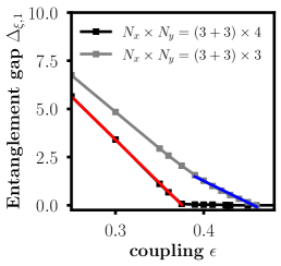
Figure 7: Details of gap closing $\Delta_{\xi,{1}}\rightarrow 0$ for $(N_{x}^{A}+N_{x}^{B})\times N_{y}=(3+3)\times 4$ and $(N_{x}^{A}+N_{x}^{B})\times N_{y}=(3+3)\times 4$ to determine the position $\epsilon_{c}$ of the confinement/deconfinement transition.

To determine the position of the confinement/deconfinement transition $\epsilon_{c}$, we consider the closing of the first entanglement gap $\Delta_{\xi,{1}}\rightarrow 0$, shown in Fig. 7 for $(N_{x}^{A}+N_{x}^{B})\times N_{y}=(3+3)\times 4$ and $(N_{x}^{A}+N_{x}^{B})\times N_{y}=(3+3)\times 4$. We use a linear fit to determine the intercept $\epsilon_{c}$. We determine the uncertainty of this linear extrapolation by removing one data point and repeating the fit. The uncertainty of this extrapolation is less than $0.01$ for all lattice sizes and is shown as error bars in Fig. 8. We use the difference between the lattices as an estimate for the finite size error, resulting, together with the uncertainty of the linear extrapolation, in $\epsilon_{c}=0.38\pm 0.09$. While an infinite volume extrapolation is not feasible with exact diagonalization, we note that the infinite volume limit result is well within the uncertainties we give.

We conducted a finite-size analysis, performing additional runs varying the size of the lattice in both $x$- and $y$-directions, with results compactly summarized in Fig. 8. These results show the robustness of the entanglement gap as an ‘order parameter’, demonstrating that finite volume effects are well under control. We note that in contrast, traditionally, the confinement/deconfinement transition is determined by expectation values of Wilson loop operators. Doing so, distinguishing volume and area law scaling, is very difficult on small lattices.

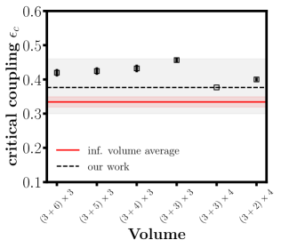
Figure 8: Finite-size analysis of the critical coupling $\epsilon_{c}$, measured as the closing of the Entanglement Gap of the Entanglement Spectrum, for different lattice sizes $(N_{x}^{A}+N_{x}^{B})\times N_{y}$.

I.3 Optimal local approximation
of the Entanglement Hamiltonian

Given the exact reduced state $\rho_{A}$, we wish to obtain an optimal local approximation $\rho_{A}\approx\sigma_{A}$ where

$$\sigma_{A}\equiv\frac{1}{Z}e^{-\sum_{\mathbf{n}\in A}\beta_{\mathbf{n}}h_{\mathbf{n}}}\;, Z=\text{Tr}\left[e^{-\sum_{\mathbf{n}\in A}\beta_{\mathbf{n}}h_{\mathbf{n}}}\right]$$ (25)

where $Z=Z(\{\beta_{\mathbf{n}}\})$, with variational parameters $\beta_{\mathbf{n}}$ and local operators $h_{\mathbf{n}}$. We obtain $\sigma_{A}$ by minimizing the relative entropy (Kullback-Leibler divergence) [108]

$$S(\rho_{A}||\sigma_{A}) \equiv\text{Tr}\left[\rho_{A}\left(\log\rho_{A}-\log\sigma_{A}\right)\right]$$

$$=-S(\rho_{A})+\log Z+\sum_{\mathbf{n}}\beta_{\mathbf{n}}\langle h_{\mathbf{n}}\rangle\;,$$ (26)

where $\langle h_{\mathbf{n}}\rangle=\text{Tr}\left[\rho_{A}h_{\mathbf{n}}\right]$ are the expectation values in the state $\rho_{A}$ and $S(\rho_{A})$ is the corresponding von Neumann entropy. Motivated by the BW theorem, in practice we choose all contributions of the subsystem to the Hamiltonian, i.e. all electric and magnetic energy terms fully supported in $A$, as the operators $h_{\mathbf{n}}$. It is well known [108] that the relative entropy is a convex function with $S(\rho_{A}||\sigma_{A})\geq 0$ where equality is obtained if $\rho_{A}=\sigma_{A}$. While this enables an efficient minimization, we nevertheless need to evaluate $Z$ several hundreds to thousands of times in order to obtain convergence. Since our numerical simulations are based on exact diagonalization, we are limited to relatively small system sizes which we have slightly increased by incorporating translational invariance of the variational parameters parallel to the entanglement cut.

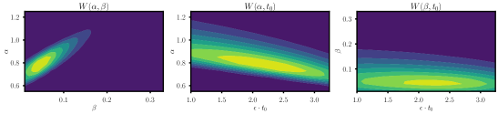
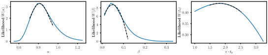
Figure 9: Top: Partially integrated Likelihood distributions $W(\alpha,\beta)$, $W(\alpha,t_{0})$ and $W(\beta,t_{0})$. Bottom: Integrated Likelihood distributions $W(\alpha)$, $W(\beta)$ and $W(t_{0})$. Dashed lines indicate a Gaussian fit.

I.4 Level Spacing Statistics
of the Entanglement Spectrum

To extract level spacing statistics of the ES, we first project the reduced density matrix into symmetry sectors. As outlined above, $2^{2N_{y}}$ sectors are given by the values of the electric flux into the subsystem through both boundaries, i.e. $\sigma^{x}_{\scriptscriptstyle(-1,n_{y}),x}$ and $\sigma^{x}_{\scriptscriptstyle(N^{A}_{x}-1,n_{y}),x}$. Because of Gauss law on the boundary, these can be written in terms of operators inside system A, e.g.

$$\sigma^{x}_{\scriptscriptstyle(-1,n_{y}),x}=\sigma^{x}_{\scriptscriptstyle(0,n_{y}),x}\sigma^{x}_{\scriptscriptstyle(0,n_{y}),y}\sigma^{x}_{\scriptscriptstyle(0,n_{y}-1),y}$$ (27)

for the left boundary of $A$. In the dual theory with entanglement cuts these operators are given as Eq. (I.1) on the left boundary at $n_{x}=0$, and on the right boundary at $n_{x}=N_{x}^{A}-1$ by Eq. (I.1). Projectors are simply constructed as

$$P_{\mathord{\uparrow}/\mathord{\downarrow},n_{y}}=\frac{1}{2}(1\pm\sigma^{x}_{\scriptscriptstyle(-1,n_{y}),x})$$ (28)

and likewise for the other boundary. We label symmetry sectors by a string of symbols $\mathord{\downarrow}\mathord{\uparrow}\dots\mathord{\uparrow}$ of length $2^{2N_{y}}$, starting at $n_{y}=0$ of the left entanglement cut and ending at $N_{y}-1$ of the right boundary.

The symmetry related to $\tilde{V}_{x}=\prod_{\mathbf{n}\in\tilde{\mathcal{C}}}\sigma^{x}_{\mathbf{n,i}}$, where $\tilde{\mathcal{C}}$ is a path from one boundary to the other, is projected on by $P=\frac{1}{2}(1\pm\tilde{V}_{x})$ and sectors are labelled by $\pm$. Together one of $2^{2N_{y}+1}$ symmetry sectors is labelled by a string, e.g. $\mathord{\downarrow}\mathord{\uparrow}\dots\mathord{\uparrow}+$.

We then compute the gap ratio

$$r_{n}\equiv\frac{\text{min}(\delta_{n},\delta_{n-1})}{\text{max}(\delta_{n},\delta_{n-1})}$$ (29)

where $\delta_{n}\equiv\xi_{n}-\xi_{n-1}\geq 0$ of the ES $\xi_{n}$, between every state $n$ within each symmetry sector and plot the distribution of gap ratios combined from all sectors. We compare with a Poissonian distribution, Gaussian Orthogonal Ensemble (GOE) and Gaussian Unitary Ensemble (GUE) [26]

$$\mathcal{P}^{\rm Poiss.}(r)=\frac{2}{(1+r)^{2}}\,,$$

$$\mathcal{P}^{\rm GOE}(r)=\frac{27}{4}\frac{r+r^{2}}{(1+r+r^{2})^{5/2}}$$

$$\mathcal{P}^{\rm GUE}(r)=\frac{81}{2}\frac{\sqrt{3}}{\pi}\frac{(r+r^{2})^{2}}{(1+r+r^{2})^{4}}\,.$$ (30)

with average $\langle r\rangle^{\rm Poisson}\approx 0.38$, $\langle r\rangle^{\rm GOE}\approx 0.52$ and $\langle r\rangle^{\rm GUE}\approx 0.60$.

For the level spacing ratio we remove the dependence on the mean level density by first unfolding the spectrum $\xi_{n}\rightarrow\bar{\xi}_{n}$ as in [79]. We then define $s_{n}\equiv\bar{\xi}_{n}-\bar{\xi}_{n-1}$ and compare with

$$\mathcal{P}^{\rm Poiss.}(s)=e^{-s}$$

$$\mathcal{P}^{\rm GOE}(s)=\frac{\pi}{2}s\,e^{-\frac{\pi}{4}s^{2}}$$

$$\mathcal{P}^{\rm GUE}(s)=\frac{32}{\pi^{2}}\,s^{2}\,e^{-\frac{4}{\pi}s^{2}}\,.$$ (31)

I.5 Scaling Analysis

Outlined below are the details of the statistical analysis to determine the scaling coefficients $\alpha,\beta$, closely following [51]. Assuming a scaling form of the Schmidt spectrum of states $n$ in an intermediate time window,

$$P(n,t)=\tau^{-\alpha}P(\tau^{\beta}n)\,,$$ (32)

where $\tau=\epsilon(t-t_{0})$ and $t_{0}$ is the onset time of self-similarity, we determine $\alpha,\,\beta$ and $t_{0}$ by the following procedure: First, we define a reference function

$$f_{\rm ref}(t,\hat{n}=\tau^{\beta}n)=\log\{\tau^{-\alpha}_{\rm ref}P(\tau_{\rm ref}^{\beta}n)\}\,.$$ (33)

where $\epsilon\cdot t_{\rm ref}=6$. We compare this reference function to a number of $N_{t}$ test times,

$$f_{\rm test}(t,\hat{n})=\log\{\tau^{-\alpha}_{\rm test}P(\tau_{\rm test}^{\beta}n)\}\,.$$ (34)

where $\epsilon\cdot t_{\rm test}\in\{8,12,16,24,30,40,50\}$. We quantify deviation from ideal scaling in terms of

$$\chi^{2}(\alpha,\beta,t_{0})=\frac{1}{N_{t}}\sum_{t\in t_{\rm test}}\frac{\int\frac{d\hat{n}}{\hat{n}}(f_{\rm ref}(\hat{n})-f_{\rm test}(\hat{n}))^{2}}{\int\frac{d\hat{n}}{\hat{n}}(f_{\rm ref}(\hat{n}))^{2}}\,.$$ (35)

and restrict $n$ to the scaling window $n\in[130,1300]$ which we vary to determine the error of our fit. We checked that a different choice of test times within the scaling regime does not change the outcome of our fit. Note that the spectrum $\hat{n}$ is discrete, and thus the integral should be replaced by a sum, but the same equation holds in the limit of a continuous spectrum.

The likelihood of a given set of parameter to reproduce the ideal rescaling function is given by

$$W(\alpha,\beta,t_{0})=\frac{1}{\mathcal{N}}\exp\Big{(}-\chi^{2}(\alpha,\beta,t_{0})/\chi^{2}_{\rm min}\Big{)}$$ (36)

where $\mathcal{N}$ is a normalization, and $\chi^{2}_{\rm min}$ is the minimum of Eq. (35), $\chi_{\rm min}=4\cdot 10^{-5}$, which is obtained for $\alpha\approx 0.75$, $\beta\approx 0.04$ and $\epsilon\cdot t_{0}\approx 2.0$, shown in the main text.

Fig. 9 (top) shows the reduced likelihood distributions $W(\alpha,\beta)$, $W(\alpha,t_{0})$ and $W(\beta,t_{0})$ obtained by integrating one of three variables, i.e. $W(\alpha,\beta,)=\int dt_{0}W(\alpha,\beta,t_{0})$. Fig. 9 (bottom) shows the integrated distributions $W(\alpha)$, $W(\beta)$ and $W(t_{0})$, and the values we quote in the main text are determined from these distributions,

$$\alpha=0.8\pm 0.2\,\quad\beta=0.0\pm 0.1\,,$$

and $\epsilon\cdot t_{0}=1.8\pm 0.5$. These were determined by fitting Fig. 9 (bottom) locally with Gaussians.

Figure 10: Scaling coefficients $\alpha$ and $\beta$ extracted from the Entanglement Spectrum of various lattice sizes.

We performed additional runs to estimate finite-volume errors in determining $\alpha$ and $\beta$, with results compactly summarized in Fig. 10. The errors quoted here are determined from this analysis, and also include the error from varying the fit range of the statistical analysis. While finite volume effects are somewhat larger than for static quantities, Fig. 10 shows that they are under control, validating our results.

Resolving the scaling regime with higher precision, in particular where it extends into the low lying part of the ES, would require lattices with larger subsystem size of $A$ (and consequently also $V_{B}\gg V_{A}$, or at least $V_{B}>V_{A}$, otherwise the Schmidt spectrum of A is cut off). This is challenging given the exponentially larger cost when using exact diagonalization.

References

Eisert et al. [2015]J. Eisert, M. Friesdorf, and C. Gogolin, Nature Physics 11, 124 (2015).
Schachenmayer et al. [2015]J. Schachenmayer, L. Pollet, M. Troyer, and A. J. Daley, EPJ Quantum
Technology 2, 1
(2015).
Eigen et al. [2018]C. Eigen, J. A. Glidden,
R. Lopes, E. A. Cornell, R. P. Smith, and Z. Hadzibabic, Nature 563, 221 (2018).
Nandkishore and Huse [2015]R. Nandkishore and D. A. Huse, Annu.
Rev. Condens. Matter Phys. 6, 15 (2015).
Gornyi et al. [2005]I. Gornyi, A. Mirlin, and D. Polyakov, Physical review
letters 95, 206603
(2005).
Oganesyan and Huse [2007]V. Oganesyan and D. A. Huse, Physical
review b 75, 155111
(2007).
Borgonovi et al. [2016]F. Borgonovi, F. M. Izrailev, L. F. Santos, and V. G. Zelevinsky, Physics Reports 626, 1
(2016).
Micha and Tkachev [2004]R. Micha and I. I. Tkachev, Physical Review D 70, 043538 (2004).
Baier et al. [2001]R. Baier, A. H. Mueller,
D. Schiff, and D. T. Son, Physics Letters B 502, 51 (2001).
Berges [2002]J. Berges, Nuclear Physics A 699, 847 (2002).
Arrizabalaga et al. [2005]A. Arrizabalaga, J. Smit, and A. Tranberg, Physical Review
D 72, 025014 (2005).
Balasubramanian et al. [2011]V. Balasubramanian, A. Bernamonti, J. de Boer,
N. Copland, B. Craps, E. Keski-Vakkuri, B. Müller, A. Schäfer, M. Shigemori, and W. Staessens, Physical Review D 84, 026010 (2011).
Grozdanov et al. [2016]S. Grozdanov, N. Kaplis, and A. O. Starinets, Journal of High
Energy Physics 2016, 1
(2016).
Berges et al. [2020]J. Berges, M. P. Heller,
A. Mazeliauskas, and R. Venugopalan, arXiv preprint
arXiv:2005.12299 (2020).
Deutsch [1991]J. M. Deutsch, Physical Review A 43, 2046 (1991).
Srednicki [1994]M. Srednicki, Physical Review E 50, 888 (1994).
D’Alessio et al. [2016]L. D’Alessio, Y. Kafri,
A. Polkovnikov, and M. Rigol, Advances in Physics 65, 239 (2016).
Li and Haldane [2008]H. Li and F. D. M. Haldane, Physical review letters 101, 010504 (2008).
Deutsch et al. [2013]J. Deutsch, H. Li, and A. Sharma, Physical Review E 87, 042135 (2013).
Yang et al. [2015]Z.-C. Yang, C. Chamon,
A. Hamma, and E. R. Mucciolo, Physical review letters 115, 267206 (2015).
Khemani et al. [2014]V. Khemani, A. Chandran,
H. Kim, and S. L. Sondhi, Physical Review E 90, 052133 (2014).
Geraedts et al. [2016]S. D. Geraedts, R. Nandkishore, and N. Regnault, Physical Review B 93, 174202 (2016).
Turner et al. [2018]C. J. Turner, A. A. Michailidis, D. A. Abanin, M. Serbyn, and Z. Papić, Nature Physics 14, 745 (2018).
Zhu et al. [2020]W. Zhu, Z. Huang, Y.-C. He, and X. Wen, Physical review letters 124, 100605 (2020).
Sels and Polkovnikov [2021]D. Sels and A. Polkovnikov, arXiv preprint arXiv:2105.09348 (2021).
Atas et al. [2013]Y. Atas, E. Bogomolny,
O. Giraud, and G. Roux, Physical review letters 110, 084101 (2013).
Giraud et al. [2020]O. Giraud, N. Macé,
E. Vernier, and F. Alet, arXiv preprint arXiv:2008.11173
(2020).
Buividovich and Polikarpov [2008]P. Buividovich and M. Polikarpov, Physics Letters B 670, 141 (2008).
Casini et al. [2014]H. Casini, M. Huerta, and J. A. Rosabal, Physical Review
D 89, 085012 (2014).
Aoki et al. [2015]S. Aoki, T. Iritani,
M. Nozaki, T. Numasawa, N. Shiba, and H. Tasaki, Journal of High Energy Physics 2015, 1 (2015).
Ghosh et al. [2015]S. Ghosh, R. M. Soni, and S. P. Trivedi, Journal of High
Energy Physics 2015, 1
(2015).
Van Acoleyen et al. [2016]K. Van Acoleyen, N. Bultinck, J. Haegeman,
M. Marien, V. B. Scholz, and F. Verstraete, Physical review letters 117, 131602 (2016).
Lin and Radicevic [2020]J. Lin and D. Radicevic, Nuclear Physics B 958, 115118 (2020).
Chen et al. [2020]J.-W. Chen, S.-H. Dai, and J.-Y. Pang, Nuclear Physics B 951, 114892 (2020).
Wegner [1971]F. J. Wegner, Journal of Mathematical Physics 12, 2259 (1971).
Horn et al. [1979]D. Horn, M. Weinstein, and S. Yankielowicz, Physical Review
D 19, 3715 (1979).
Radievic [2016]D. Radievic, Journal of High Energy Physics 2016, 1 (2016).
Kokail et al. [2020]C. Kokail, R. van Bijnen,
A. Elben, B. Vermersch, and P. Zoller, arXiv preprint arXiv:2009.09000 (2020).
Bisognano and Wichmann [1975]J. J. Bisognano and E. H. Wichmann, Journal of Mathematical Physics 16, 985 (1975).
Bisognano and Wichmann [1976]J. J. Bisognano and E. H. Wichmann, Journal of mathematical physics 17, 303 (1976).
Rakovszky et al. [2019]T. Rakovszky, S. Gopalakrishnan, S. Parameswaran, and F. Pollmann, Physical Review B 100, 125115 (2019).
Chang et al. [2019]P.-Y. Chang, X. Chen,
S. Gopalakrishnan, and J. Pixley, Physical review letters 123, 190602 (2019).
Chamon et al. [2014]C. Chamon, A. Hamma, and E. R. Mucciolo, Physical review
letters 112, 240501
(2014).
Yang et al. [2019]Z.-C. Yang, K. Meichanetzidis, S. Kourtis, and C. Chamon, Physical Review B 99, 045132 (2019).
Serbyn et al. [2016]M. Serbyn, A. A. Michailidis, D. A. Abanin, and Z. Papić, Physical review letters 117, 160601 (2016).
Mierzejewski et al. [2013]M. Mierzejewski, T. Prosen, D. Crivelli, and P. Prelovšek, Physical review
letters 110, 200602
(2013).
Bertini et al. [2019]B. Bertini, P. Kos, and T. Prosen, Physical Review X 9, 021033 (2019).
Berges et al. [2014a]J. Berges, K. Boguslavski,
S. Schlichting, and R. Venugopalan, Physical Review
D 89, 074011 (2014a).
Berges et al. [2014b]J. Berges, K. Boguslavski,
S. Schlichting, and R. Venugopalan, Journal of High
Energy Physics 2014, 1
(2014b).
Mace et al. [2020]M. Mace, N. Mueller,
S. Schlichting, and S. Sharma, Physical review letters 124, 191604 (2020).
Meurice et al. [2020]Y. Meurice, R. Sakai, and J. Unmuth-Yockey, arXiv preprint
arXiv:2010.06539 (2020).
Bañuls and Cichy [2020]M. C. Bañuls and K. Cichy, Reports
on Progress in Physics 83, 024401 (2020).
Robaina et al. [2021]D. Robaina, M. C. Bañuls, and J. I. Cirac, Physical Review Letters 126, 050401 (2021).
Kielpinski et al. [2002]D. Kielpinski, C. Monroe, and D. J. Wineland, Nature 417, 709 (2002).
Monroe [2002]C. Monroe, Nature 416, 238
(2002).
Blais et al. [2004]A. Blais, R.-S. Huang,
A. Wallraff, S. M. Girvin, and R. J. Schoelkopf, Physical Review A 69, 062320 (2004).
Cirac and Zoller [2012]J. I. Cirac and P. Zoller, Nature Physics 8, 264 (2012).
Hauke et al. [2012]P. Hauke, F. M. Cucchietti, L. Tagliacozzo, I. Deutsch, and M. Lewenstein, Reports on Progress in Physics 75, 082401 (2012).
Preskill [2018]J. Preskill, Quantum 2, 79 (2018).
Martinez et al. [2016]E. A. Martinez, C. A. Muschik, P. Schindler,
D. Nigg, A. Erhard, M. Heyl, P. Hauke, M. Dalmonte,
T. Monz, P. Zoller, et al., Nature 534, 516 (2016).
Klco et al. [2018]N. Klco, E. Dumitrescu,
A. McCaskey, T. Morris, R. Pooser, M. Sanz, E. Solano, P. Lougovski, and M. Savage, arXiv preprint
arXiv:1803.03326 (2018).
Zache et al. [2018]T. V. Zache, F. Hebenstreit,
F. Jendrzejewski, M. Oberthaler, J. Berges, and P. Hauke, Quantum Science and Technology (2018).
Davoudi et al. [2020a]Z. Davoudi, M. Hafezi,
C. Monroe, G. Pagano, A. Seif, and A. Shaw, Physical Review Research 2, 023015 (2020a).
Mil et al. [2020]A. Mil, T. V. Zache,
A. Hegde, A. Xia, R. P. Bhatt, M. K. Oberthaler, P. Hauke, J. Berges, and F. Jendrzejewski, Science 367, 1128 (2020).
de Jong et al. [2021]W. A. de Jong, K. Lee,
J. Mulligan, M. Płoskoń, F. Ringer, and X. Yao, arXiv preprint arXiv:2106.08394 (2021).
Schweizer et al. [2019]C. Schweizer, F. Grusdt,
M. Berngruber, L. Barbiero, E. Demler, N. Goldman, I. Bloch, and M. Aidelsburger, Nature Physics 15, 1168 (2019).
Barbiero et al. [2019]L. Barbiero, C. Schweizer,
M. Aidelsburger, E. Demler, N. Goldman, and F. Grusdt, Science advances 5, eaav7444 (2019).
Homeier et al. [2021]L. Homeier, C. Schweizer,
M. Aidelsburger, A. Fedorov, and F. Grusdt, Physical Review B 104, 085138 (2021).
Note [1] are electric flux loops winding around the
periodic - and -directions of the torus, so called ‘ribbon’
operators [105, 95], see also [106, 107].
Bravyi et al. [2011]S. Bravyi, D. P. DiVincenzo, and D. Loss, Annals
of physics 326, 2793
(2011).
Patkós and Deak [1981]A. Patkós and F. Deak, Zeitschrift für Physik C Particles and Fields 9, 359 (1981).
Dass et al. [1982]N. H. Dass, A. Patkos, and F. Deák, Nuclear Physics B 205, 414 (1982).
Patkos and Dass [1982]A. Patkos and N. H. Dass, Physics
Letters B 119, 391
(1982).
Blöte and Deng [2002]H. W. Blöte and Y. Deng, Physical
Review E 66, 066110
(2002).
Weinberg and Bukov [2018]P. Weinberg and M. Bukov, arXiv
preprint arXiv:1804.06782 (2018).
Garrison and Grover [2018]J. R. Garrison and T. Grover, Physical Review X 8, 021026 (2018).
Drouffe et al. [1979]J. Drouffe, C. Itzykson, and J. Zuber, Nuclear Physics
B 147, 132 (1979).
Mathur and Sreeraj [2015]M. Mathur and T. Sreeraj, Physical Review D 92, 125018 (2015).
Mathur [2005]M. Mathur, Journal of Physics A: Mathematical and General 38, 10015 (2005).
Mathur [2007]M. Mathur, Nuclear Physics B 779, 32 (2007).
Anishetty and Raychowdhury [2014]R. Anishetty and I. Raychowdhury, Physical Review D 90, 114503 (2014).
Mathur et al. [2010]M. Mathur, I. Raychowdhury, and R. Anishetty, Journal of mathematical physics 51, 093504 (2010).
Raychowdhury and Stryker [2020b]I. Raychowdhury and J. R. Stryker, Physical Review Research 2, 033039 (2020b).
Tekur and Santhanam [2020]S. H. Tekur and M. Santhanam, Physical Review Research 2, 032063 (2020).
Brenes et al. [2018]M. Brenes, M. Dalmonte,
M. Heyl, and A. Scardicchio, Physical review letters 120, 030601 (2018).
Kitaev [2003]A. Y. Kitaev, Annals
of Physics 303, 2
(2003).
Satzinger et al. [2021]K. Satzinger, Y. Liu,
A. Smith, C. Knapp, M. Newman, C. Jones, Z. Chen, C. Quintana, X. Mi,
A. Dunsworth, et al., arXiv
preprint arXiv:2104.01180 (2021).
Kasper et al. [2020]V. Kasper, G. Juzeliūnas, M. Lewenstein, F. Jendrzejewski, and E. Zohar, New
Journal of Physics 22, 103027 (2020).
Wen [2004]X.-G. Wen, Quantum field theory of
many-body systems: from the origin of sound to an origin of light and
electrons (Oxford University Press on Demand, 2004).
Kharzeev and Levin [2017]D. E. Kharzeev and E. M. Levin, Physical Review D 95, 114008 (2017).
Mueller et al. [2020]N. Mueller, A. Tarasov, and R. Venugopalan, Physical Review
D 102, 016007 (2020).
Tu et al. [2020]Z. Tu, D. E. Kharzeev, and T. Ullrich, Physical review
letters 124, 062001
(2020).
Pichler et al. [2016]H. Pichler, G. Zhu,
A. Seif, P. Zoller, and M. Hafezi, Physical Review X 6, 041033 (2016).
Dalmonte et al. [2018]M. Dalmonte, B. Vermersch, and P. Zoller, Nature
Physics 14, 827
(2018).
Elben et al. [2020]A. Elben, R. Kueng,
H.-Y. R. Huang, R. van Bijnen, C. Kokail, M. Dalmonte, P. Calabrese, B. Kraus, J. Preskill, P. Zoller, et al., Physical Review Letters 125, 200501 (2020).
Sachdev [2018]S. Sachdev, Reports on Progress in Physics 82, 014001 (2018).
Michael [1987]C. Michael, Journal of Physics G: Nuclear Physics 13, 1001 (1987).
van Baal and Koller [1987]P. van
Baal and J. Koller, Annals of
Physics 174, 299
(1987).
Kullback and Leibler [1951]S. Kullback and R. A. Leibler, The
annals of mathematical statistics 22, 79 (1951).