An Instance-Dependent Simulation Framework for Learning with Label Noise

Abstract

We propose a simulation framework for generating instance-dependent noisy labels via a pseudo-labeling paradigm. We show that the distribution of the synthetic noisy labels generated with our framework is closer to human labels compared to independent and class-conditional random flipping. Equipped with controllable label noise, we study the negative impact of noisy labels across a few practical settings to understand when label noise is more problematic. We also benchmark several existing algorithms for learning with noisy labels and compare their behavior on our synthetic datasets and on the datasets with independent random label noise. Additionally, with the availability of annotator information from our simulation framework, we propose a new technique, Label Quality Model (LQM), that leverages annotator features to predict and correct against noisy labels. We show that by adding LQM as a label correction step before applying existing noisy label techniques, we can further improve the models’ performance. The synthetic datasets that we generated in this work are released at https://github.com/deepmind/deepmind-research/tree/master/noisy_label.

1 Introduction

In many applications, training machine learning models requires labeled data. In practice, the training data labeled by human raters are often noisy, leading to inferior model performance. The study of learning in the presence of label noise dates back to the eighties (Angluin and Laird, 1988), and still receives significant attention in recent years (Natarajan et al., 2013; Reed et al., 2014; Malach and Shalev-Shwartz, 2017; Han et al., 2018; Li et al., 2020a).

In the research community, some datasets with real noisy human ratings are available, such as Clothing 1M (Xiao et al., 2015), Food 101-N (Lee et al., 2018) (only a small subset has clean labels), WebVision (Li et al., 2017a), and CivilComments (Borkan et al., 2019), which allow testing approaches that address label noise. However, since the level and type of label noise in these datesets cannot be controlled, it becomes hard to conduct ablation study to understand the impact of noisy labels. As a result, the majority of research work in this area uses benchmark datasets generated by simulations. For example, many prior works simulate noisy labels by flipping the labels according to certain transition matrix (Natarajan et al., 2013; Khetan et al., 2017; Patrini et al., 2017; Han et al., 2018; Hendrycks et al., 2018), independently from the model inputs, e.g., the raw images. However, this type of random label noise may not be an ideal way to simulate noisy labels, since the errors in human ratings are often instance-dependent, i.e., harder examples are easier to get wrong labels, whereas the noisy labels generated by random flipping do not have this type of dependency, even if the transition matrix is asymmetric, i.e., class-conditional. In addition, in many applications, we often have additional features of the raters, such as tenure, historical biases, and expertise level (Cabitza et al., 2020). Leveraging these features properly can potentially lead to better model performance. However, neither the commonly used public datasets with human ratings nor the synthetic datasets created by random label noise have such rater features available.

In this work, we focus on creating simulation benchmarks for the research on label noise. We propose a method that is instance-dependent, easy to implement, and can convert any commonly used public dataset with clean labels into a noisy label dataset with additional rater features. More specifically, we propose a simulation method based on a pseudo-labeling paradigm: given a dataset with clean labels, we use a subset of it to train a set of models (rater models), and use them to label the rest of the data. In this way, we obtain a dataset whose size is smaller than the original one with clean labels, but with multiple instance-dependent noisy labels. Moreover, some characteristics of the rater models, such as the number of training epochs, the number of samples used, the validation performance metrics, and the number of parameters in the model can be used as a proxy for the rater features.

We note that this simulation approach is very similar to self-training in semi-supervised learning (Chapelle et al., 2006). In the research on label noise, methods inspired by semi-supervised learning have been adopted in several prior works for training robust models (Han et al., 2018; Li et al., 2020a) or generate synthetic noisy label dataset (Lee et al., 2019; Robinson et al., 2020). We intend to exploit this approach for both providing a comprehensive study of how practical label noise affects the performance of machine learning models, and the research of better training algorithm in the presence of label noise. Our main contributions are summarized as follows:

• We propose a pseudo-labeling simulation framework for learning with label noise. We provide detailed description, including the generation of rater features. We also evaluate the synthetic datasets generated by our framework and show that the distribution of noise labels in our datasets is closer to human labels compared to independent and class-conditional random flipping (Section 2).

• We study the negative impact of label noise on deep learning models using our synthetic datasets. We find that noisy labels are more detrimental under class imbalanced settings, when pretraining is not used, and on tasks that are easier to learn with clean labels (Section 3).

• We benchmark existing approaches to tackling label noise using our synthetic datasets. We find that the behavior of these techniques on the our synthetic datasets is different from the datasets generated by independent random label flipping. With the same fraction of mislabeled data, our datasets tend to be harder than datasets with random label noise for binary classification tasks; however, we observe the opposite trend for multi-class tasks (Section 4).

• We propose a label correction approach, named Label Quality Model (LQM), that leverages rater features to significantly improve model performance. We also show that LQM can be combined with other existing noisy label techniques to further improve the performance (Section 5).

2 Generating Synthetic Datasets with Instance-Dependent Label Noise

In this section, we discuss the formulation of generating synthetic noisy labels, and provide details for the dataset generation procedure and the methods we use to evaluate whether the synthetic datasets share certain characteristics of real human labeled data.

2.1 Formulation

We consider a $K$-class classification problem with input space $\mathcal{X}$ and label space $\mathcal{Y}=\{1,\ldots,K\}$. In addition, we assume that there is a rater space $\mathcal{R}$, with each element being the feature of a rater who can label any element in $\mathcal{X}$. Suppose that there is an unknown distribution over $\mathcal{X}\times\mathcal{Y}\times\mathcal{R}\times\mathcal{Y}$, and each tuple $(x,y^{*},r,y)$ in this space corresponds to the input feature of an example $x$, clean label of the example $y^{*}$, a rater $r$, and the label $y$ provided by the rater.

The problem of generating synthetic noisy labels can be modeled as generating a noisy label $y$ given a pair of input feature and clean label $y^{*}$. Ideally, the probability distribution of the noisy label $y$ should depend on all of $x$, $y^{*}$, and $r$, i.e., we should generate $y$ according to $p(y\mid x,y^{*},r)$. This means that the label noise should depend on the input—harder and more nuanced examples such as blurred images are more likely to have incorrect labels, as well as the rater—raters with higher expertise level are less likely to make mistakes.

However, many prior studies on generating synthetic noisy labels ignore such dependency on $x$ and $r$ and only generate $y$ according to $y^{*}$. Here, we specify three approaches for generating noisy labels.

• Independent random flipping. In this method, with probability $\delta$, the label of each example is flipped to an incorrect one, uniformly chosen from all the other $K-1$ labels (Zhang et al., 2021a; Rolnick et al., 2017; Han et al., 2018). The method is sometimes called symmetric label noise. More specifically, we have

  $$p(y=k\mid y^{*})=(1-\delta)\mathbf{1}(k=y^{*})+\frac{\delta}{K-1}\mathbf{1}(k\neq y^{*}).$$

• Class-conditional random flipping. In this method, we assume that there is a stochastic matrix $T\in\mathbb{R}^{K\times K}$. The $i$-th row of $T$ corresponds to the probability distribution of the noisy label $y$ given that the clean label $y^{*}=i$, i.e.,

  $$p(y=j\mid y^{*}=i)=T_{i,j}.$$

  This method is sometimes called the asymmetric label noise, and is usually considered more practical than symmetric noise, since classes that are semantically close are more likely to be confused than classes that have clearer decision boundaries. As mentioned in Section 1, this method has been used in many prior works (Angluin and Laird, 1988; Han et al., 2018; Zhang et al., 2017; Wang et al., 2019; Jiang et al., 2018); the matrix can be designed with human knowledge or estimated from a small subset of clean data (Patrini et al., 2017; Hendrycks et al., 2018). Here, we emphasize that the noisy labels in class-conditional label flipping still do not depend on the input feature $x$ and the rater $r$.

• Instance-dependent, i.e., generating noisy labels according to $p(y\mid x,y^{*},r)$. The method that we propose in this paper satisfies this criterion. Similar problems have been considered in several very recent works (Berthon et al., 2021; Zhu et al., 2021; Zhang et al., 2021b).

2.2 Dataset generation

In our framework, we first identify a public dataset that we would like to generate noisy labels for, e.g., CIFAR10 (Krizhevsky and Hinton, 2009) for image classification. We observe that many public datasets already have default training, validation, and test splits. For those without a validation split, we can randomly partition the training data into training and validation splits. We note that in our paper we assume that public datasets have “clean” labels. We acknowledge that many widely used public datasets such as CIFAR10 or ImageNet (Deng et al., 2009) may have mislabeled data points (Northcutt et al., 2021b); however, the amount of label noise in these public datasets is significantly smaller than what the noisy label research community usually consider (Han et al., 2018; Lee et al., 2019), including our work. Therefore, we believe it is reasonable to consider the labels in public datasets as clean, i.e., less noisy, labels, and we do not expect the label noise in public datasets changes the conclusions in our paper.

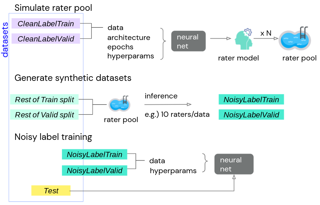
Figure 1: Pseudo-labeling paradigm for simulating instance-dependent noisy labels.

We further split the training and validation splits into two disjoint sets, respectively. More specifically, we partition the training set into CleanLabelTrain and NoisyLabelTrain, and the validation set into CleanLabelValid and NoisyLabelValid. We use the data in CleanLabelTrain with clean labels to train a set of rater models, which can be any standard models for the problem domain. The data in the CleanLabelValid split can be used to evaluate the rater models. For example, the test accuracy with respect to the clean labels on the CleanLabelValid split can be used as a feature of a rater model. We can obtain a pool of rater models by choosing different architectures, training epochs, and other training configurations, which can all be used as rater features. Then we use all or a subset of models from the rater pool to run inference on the data in the NoisyLabelTrain and NoisyLabelValid splits. In this way we obtain multiple noisy labels for every data in these two splits, and we replace the clean labels with these noisy labels. We note that in this paper, when we run inference using a rater model, we use the “hard predictions”, i.e., each example is labeled according to the largest logit of the rater model’s prediction. It is also valid to treat the output of the rater models as a distribution over the classes and sample a noisy label from it. We find that in order to control the amount of label noise in these two splits, it is important to train a diverse set of rater models using different combinations of architectures, training steps, learning rate, and batch size. The details for the rater models that we use throughout this paper are provided in Appendix A. To perform label noise research, we can use the NoisyLabelTrain split to train models and use the NoisyLabelValid split for hyperparameter tuning. For the Test split, we use the original clean labels. We illustrate our framework in Figure 1. To summarize, we split the dataset into 5 disjoint sets:

• CleanLabelTrain: a set of data with clean labels, used for training rater models.

• CleanLabelValid: a set of data with clean labels, used for evaluating rater models.

• NoisyLabelTrain: a set of data with multiple noisy labels (prediction of rater models), used for model training with noisy labels.

• NoisyLabelValid: a set of data with multiple noisy labels (prediction of rater models), used for hyperparameter tuning when training on the NoisyLabelTrain split.

• Test: a set of data with clean labels for final evaluation of the model trained on NoisyLabelTrain.

In most of our experiments, the sizes of the CleanLabelTrain and NoisyLabelTrain splits are around 50% of the original training and validation splits. However, this ratio can be adjusted depending on the problem of interest. For a synthetic dataset with multiple noisy labels, i.e., the NoisyLabelTrain and NoisyLabelValid splits, we use the following two metrics to measure the amount of noise in the dataset: (1) overall rater error rate, which is defined as the fraction of the incorrect labels among all the labels given by all the raters, and (2) Krippendorff’s alpha (k-alpha) (Hayes and Krippendorff, 2007), which measures the agreement between the raters. We note that the computation of Krippendorff’s alpha does not require the clean labels. Usually, datasets with higher k-alpha are less noisy. All model training in this and the following sections are performed on TPUs in our internal cluster.

2.3 Dataset evaluation

Once we have the synthetic datasets, the next step is to compare them with other simulation methods. More specifically, we make comparison with independent random flipping and class-conditional random flipping, and show that the distribution of the noisy labels that we generate is closer to real human labels. We use the following metric named mean total variation distance to measure the difference between the distribution of noisy labels in different datasets.

Let $D_{1}=\{(x_{i},y_{i}^{1})\}_{i=1}^{n}$ and $D_{2}=\{(x_{i},y_{i}^{2})\}_{i=1}^{n}$ be two noisy label datasets with the same set of input features. We consider soft labels, i.e., $y_{i}^{1},y_{i}^{2}\in\mathbb{R}^{K}$ are probability distributions over $\{1,\ldots,K\}$. The mean total variation distance between datasets $D_{1}$ and $D_{2}$ is defined as $d_{TV}(D_{1},D_{2}):=\frac{1}{2n}\sum_{i=1}^{n}\|y_{i}^{1}-y_{i}^{2}\|_{1}$.

We use the CIFAR10-H dataset (Peterson et al., 2019) as the real human labels. This dataset contains the 10K data points from the CIFAR10 test split with around $50$ labels for each data. To create the synthetic noisy label datasets using our framework in Section 2.2, we train rater models using the CleanLabelTrain  split and run inference on the CIFAR10 test data. We create three synthetic datasets with low, medium and high amount of noise. We train $10$ rater models for each dataset and thus each example has $10$ noisy labels. The rater error rates—defined as the ratio of the number of incorrect labels to the total number of labels in the dataset—of the three datasets are $13.0\%$, $21.7\%$, and $52.4\%$, respectively. In the following, we call these three rater error rates the targeted error rates. Note that when we compute the rater error rates, we corrected the mislabels data in the original CIFAR10 test split according to Northcutt et al. (2021b). Details for the rater models are presented in Appendix A. With the three synthetic datasets, we then create other datasets for comparison. For real human labels, we notice that the CIFAR10-H dataset has a rater error rate around $4.8\%$, much lower than the amount of noise in our synthetic datasets. Since the goal of our framework is to create controllable noise level, we do not enforce the rate error rate of our datasets to match CIFAR10-H; instead, we upsample the incorrect labels in CIFAR10-H to match the rater error rates of our three datasets. The method of upsampling incorrect labels to create datasets with controllable amount of noise has been studied in Northcutt et al. (2021a, b). Thus, we create noise-controlled human label datasets with the three targeted error rates. For independent random flipping, we generate three datasets by choosing $\delta$ to be each of the three targeted error rates and sampling $10$ noisy labels for each data. For class-conditional random flipping, for each synthetic dataset, we first compute its class confusion matrix, and then use it as the probability transition matrix $T$ for the class-conditional setup and then sample $10$ noisy labels for each data. Then, for each targeted error rate, we compute the mean total variation distance between the real human labels and datasets with independent random flipping, class-conditional random flipping, and our synthetic dataset, respectively. The results are provided in Table 1. As we can see, for every noise level, the mean total variation distance between our synthetic dataset and the noise-controlled human labels is smaller than that of independent and class-conditional random flipping. Thus, we conclude that the distribution of noisy labels that our framework generates is closer to human labels compared to independent and class-conditional random flipping.

Table 1: Dataset evaluation. The numbers in the table are the $95\%$ confidence intervals of the mean total variation distance between the synthetic datasets generated by different methods and the noise-controlled human labeled datasets. Our datasets are closer to the human labels compared to independent and class-conditional random flipping.

noise level	low	medium	high
independent flipping	$0.207\pm 0.005$	$0.335\pm 0.008$	$0.787\pm 0.019$
class-conditional	$0.196\pm 0.005$	$0.320\pm 0.008$	$0.766\pm 0.019$
ours	0.180 $\pm$ 0.005	0.301 $\pm$ 0.008	0.742 $\pm$ 0.019

3 Impact of Label Noise on Deep Learning Models

With the instance-dependent synthetic datasets with noisy labels, our next step is to study the impact of noisy labels on deep learning models. Interestingly, there exist different views for the impact of noisy labels to deep neural networks. While most of the recent research works on noisy labels try to design algorithms that can tackle the negative impact of label noise, some other works claim that deep learning models are robust to independent random label noise (Rolnick et al., 2017; Li et al., 2020b) without using sophisticated algorithms. A prominent example is the weak supervision paradigm (Ratner et al., 2016, 2017), where massive training datasets are generated by weak raters and labeling functions. Other lines research indicate that large neural network can easily fit all the noisy labels in the training data (Zhang et al., 2021a), while smaller models may be more robust against label noise due to the regularization effect (Advani et al., 2020; Belkin et al., 2019; Northcutt et al., 2021b).

We hypothesize that the negative impact of noisy labels is problem-dependent. While in most cases the incorrect labels can impair models’ performance, the impact may depend on factors related to the data distribution and the model. In this section, we choose the following factors to measure the impact of label noise: the class imbalance, the inductive bias of the model (in particular, pretraining vs random initialization), and the difficulty of the task (test accuracy that models can achieve when clean labels are accessible). Note that for better understanding, we decouple these factors with algorithm design: In this section, we choose simple SGD-style training algorithms with cross-entropy loss and focus on analyzing the impact of label noise; the discussion on more sophisticated algorithms to tackle label noise is presented in Sections 4 and 5. We do not aim to study label aggregation methods either. Instead, in this and the following sections, given a synthetic dataset with multiple noisy labels, we generate a dataset with a single noisy label by independently and uniformly selecting a random noisy label for every data point. This is a simulation of the practical setting where we have a pool of raters and for each data, we choose a random rater from the pool and request a label.

3.1 Label Noise Has Higher Impact on More Imbalanced Datasets

One of the important characteristics of many real world datasets is that the classes are usually imbalanced. When the classes are more imbalanced, the impact of noisy labels may become more pronounced since the number of data in the minority classes is already small, and noisy labels can further corrupt these data, making the learning procedure more difficult. We validate this hypothesis in this section. We use two binary classification tasks, PatchCamelyon (PCam) (Veeling et al., 2018; Bejnordi et al., 2017) and Cats vs Dogs (CvD) (Elson et al., 2007). We generate synthetic noisy label datasets with different k-alphas, and for each of these datasets, we subsample the two classes to create several smaller datasets with different class imbalance but the same total number of data. We note that here we control the class imbalance to be the same for all of the NoisyLabelTrain, NoisyLabelValid, and Test splits. We train models with clean and noisy labels and use the difference in mean average precision (mAP) (Zhang and Zhang, 2009) and area under the precision-recall curve (AUCPR) (Raghavan et al., 1989) as the indicators for the impact of label noise. The results are shown in Figure 2. As we can see, the impact of label noise becomes more significant as the classes become more imbalanced.

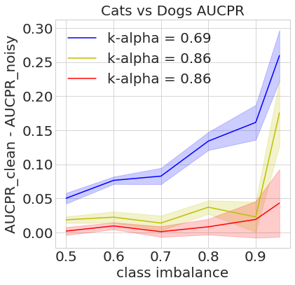
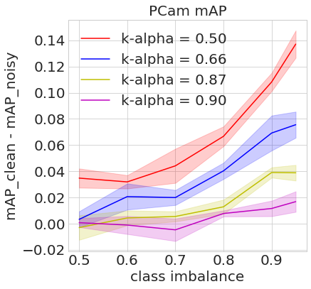
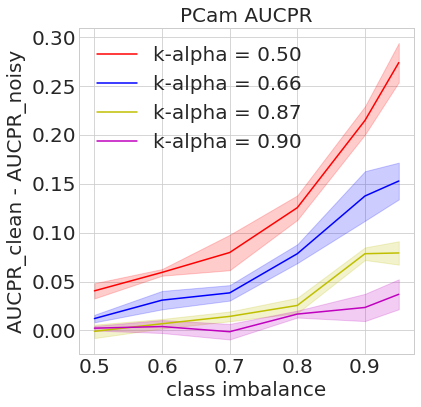
Figure 2: Impact of label noise for tasks with different class imbalance. The x-axis represents class imbalance, measured by the fraction of the majority class. For PCam, we use MobileNet-v1 (Howard et al., 2017) model, and for Cats vs Dogs, we use ResNet50 (He et al., 2016). The k-alphas correspond to the synthetic datasets before subsampling.

3.2 Pretraining Improves Robustness to Label Noise

One model training technique that is often used in practice, especially for computer vision and natural language tasks, is to pretrain the models on some large benchmark datasets and then fine-tune them using the data for specific tasks. It has been observed that model pretraining can improve robustness to independent random label noise (Hendrycks et al., 2019) and the web label noise considered by Jiang et al. (2020). Here we show that this can still be observed in our synthetic framework. A simple explanation is that model pretraining adds strong inductive bias to the models and thus they are less sensitive to a fraction of noisy labels during fine-tuning.

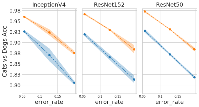
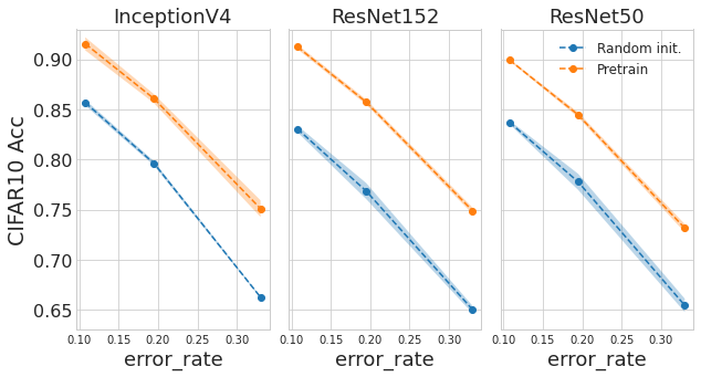
Figure 3: Pretrained models achieve better test accuracy on CvD and CIFAR10. Moreover, as the amount of label noise increases, the amount of test accuracy drop is smaller for pretraining (e.g. the slope is smaller) than training from random initialization.

We validate this hypothesis using two datasets, Cats vs Dogs (CvD) and CIFAR10. For both datasets, we generate three synthetic noisy label datasets using our framework with different rater error rates. We compare the test accuracy on the Test split (with clean labels) between the models that are trained from random initialization and those that are fine-tuned from models pretrained on ImageNet (Deng et al., 2009). We experiment with three different architectures, including Inception-v4 (Szegedy et al., 2017), ResNet152, and ResNet50 (He et al., 2016). As we can see in Figure 3, models that are pretrained on ImageNet achieve better test accuracy. In addition, for pretrained models, the test accuracy tends to drop more slowly compared to models that are trained from random initialization as we increase the amount of noise (rater error rate).

Meanwhile, we also observe that ImageNet pretraining does not improve the test accuracy under noisy labels for the PatchCamelyon dataset. This can be explained by the fact that the PatchCamelyon dataset consists of histopathologic scans of lymph node sections, and these medical images have very different distribution from the data in ImageNet. Therefore, the inductive bias that the model learned from ImageNet pretraining may not be helpful on PCam.

3.3 Easier Tasks Are More Sensitive to Label Noise

We also study the impact of label noise on tasks with different difficulty levels (the test accuracy models can achieve when clean labels are accessible). Our hypothesis here is that when a task is already hard to learn even given clean labels, then the impact of label noise is smaller. The reason can be that when a classification task is hard, the data distributions of different classes are relatively close such that even if some data are mislabeled, the final performance may not be heavily impacted. On the contrary, label noise may be more detrimental to easier tasks as the data distribution can significantly change when well-separated data points get mislabeled. We validate this hypothesis with two experiments.

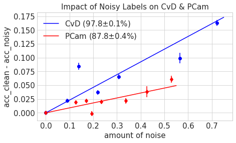
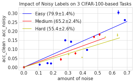
Figure 4: Impact of label noise on tasks with different difficulty levels. The numbers in the legend correspond to test accuracies when training with clean labels for every task. The x-axis represents the amount of noise, measured by $1.0-$k-alpha. The y-axis represents the negative impact of label noise, measured by the difference in test accuracy when training with clean and noisy labels. Scattered points represent the pairs of noise level and the accuracy drop, and solid lines show the linear fit of the scattered points in the same color.

Setup

Our first experiment involves two binary classification tasks, i.e., PatchCamelyon (PCam) with MobileNet-v1 (Howard et al., 2017) and Cats vs Dogs with ResNet50 (He et al., 2016). We generate synthetic noisy label datasets with different k-alphas using our framework, and compare the accuracies when the models are trained with clean and noisy labels. We observe that CvD is easier than PCam (clean label accuracy 97.8 $\pm$ 0.1% vs 87.7 $\pm$ 0.4%). In our second experiment, we design three 20-way classification tasks with the same number of data but different difficulty levels by subsampling different classes from the CIFAR100 dataset. We call the three tasks the easy, medium, and hard tasks. Details for the design of the three tasks are provided in Appendix B, and we observe that with clean labels, we can obtain test accuracies of 79.9 $\pm$ 1.4%, 65.2 $\pm$ 2.4%, and 55.4 $\pm$ 2.6% for the three tasks, respectively. We generate synthetic datasets with different amounts of noise, measured by k-alpha and use the MobileNet-v2 model (Sandler et al., 2018).

Results

We study the impact of label by measuring the absolute difference in test accuracy when training with clean and noisy labels. The results are shown in Figure 4. As we can see, the impact of noisy labels is higher on the easy task: On CvD, the drop in test accuracy grows faster as we increase the amount of label noise (indicated by $1.0-$k-alpha) compared to PCam, and similar phenomenon can be observed on the three CIFAR100-based tasks.

4 Benchmarking Noisy Label Algorithms

With our instance-dependent synthetic noisy label datasets, a natural follow-up question is how existing techniques for mitigating the impact of label noise perform on our benchmarks. In particular, we are interested in the difference of the algorithms’ performance when using our synthetic datasets and using noisy label datasets with independent random label noise. In this and the next section, when we mention a dataset uses random label noise, we mean with certain probability (rater error rate), the label of each data point is flipped to an incorrect label that is uniformly selected. This flipping event is independent of other data points and the image itself.

4.1 Experiment Setup

We compare the following $5$ algorithms: vanilla training with cross-entropy loss (Baseline), Bootstrap (Reed et al., 2014), Co-Teaching (Han et al., 2018), cross-entropy loss with Monte Carlo sampling (MCSoftMax) (Collier et al., 2020), and MentorMix (Jiang et al., 2020) on $4$ tasks: CIFAR10, CIFAR100, PatchCamelyon, and Cats vs Dogs. For each task, we generate $3$ synthetic noisy label datasets with different amount of noise using our framework. According to the rater error rate, the noisy label datasets are marked as “low”, “medium”, and “high” in Figures 5 and 6. Details for these datasets can be found in Appendix A. For each of our synthetic dataset, we generate another dataset that uses random label noise and has the same rater error rate. We compare the performance of the $5$ algorithms on these paired datasets, and aim to measure the difficulty of noisy label datasets when the label errors are generated using our framework or independent random flipping. All the experiments use the ResNet50 architecture.

4.2 Results

Interestingly, we find different behavior for tasks with different number of classes. For tasks with a large number of classes such as CIFAR100, we find that most algorithms achieve better test accuracy on our synthetic datasets compared to random label noise. On binary classification problems such as PatchCamelyon and Cats vs Dogs, however, the trend is opposite, i.e., most algorithms perform worse on our synthetic datasets. On CIFAR10, we observe mixed behavior: depending on the amount of noise and the algorithm, the test accuracy can be higher either on our synthetic datasets or those with random label noise. The results are shown in Figure 5, and exact numbers are provided in Appendix C.

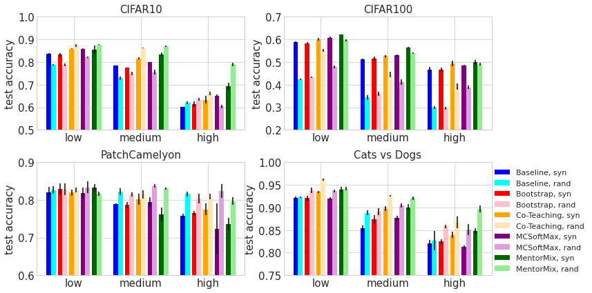
Figure 5: Benchmarking noisy label algorithms using our synthetic dataset and random label noise. Each pair of adjacent bars shows test accuracy on two datasets: our synthetic dataset (darker color) and random label noise (lighter color) with the same rater error rate. On CIFAR100, our datasets are easier than random noise, while on binary classification tasks (PCam and CvD), our datasets are harder.

Figure 6: Improvement in test accuracy using noisy label techniques. Each pair of adjacent bars shows test accuracy improvement compared to the baseline on two datasets: our synthetic dataset (darker color) and random label noise (lighter color) with the same rater error rate. In most cases, the accuracy improvement tends to be smaller under our synthetic framework.

This phenomenon can be explained as follows. For binary classification problems, in our synthetic framework, the mislabeled data are usually the ambiguous ones that located around the decision boundary. This label noise can hurt the models’ performance more since the important information around the decision boundary is corrupted. On the contrary, for tasks with a large number of classes, especially those with tree-structured classes involving a relatively small number of high level super classes and low level fine-grained classes, such as CIFAR100, in our instance-dependent simulation framework, the label mistakes are usually among similar classes. For example, an image of a certain type of mammal may be mislabeled as another mammal, but it is unlikely to be labeled as a type of vehicles. In other words, the corruption of decision boundary only happens to similar fine-grained classes in our framework. Thus, given the same fractions of incorrect labels are the same, our synthetic label noise hurts the models’ performance less compared to random noise.

Another observation is that on CIFAR10 and CIFAR100, the performance improvement obtained by noisy label algorithms when compared with the baseline is usually smaller with our synthetic datasets. The performance improvement is presented in Figure 6.

We emphasize that our results demonstrate the importance of using instance-dependent synthetic benchmarks in the research on label noise: existing algorithms exhibit different behavior on our synthetic framework and random label noise, even if the fraction of mislabeled data is kept the same, and the performance gain observed using random label noise may not directly translate to the setting that we tested.

5 Leveraging Rater Features: Label Quality Model

Existing work in the noisy label literature commonly assumes that training labels are the only output of the data curation process. In practice however, the data curation process often produces a myriad of additional features that can be leveraged in downstream training, e.g., which rater is responsible for a given label, as well as that rater’s tenure, historical errors, and time spent on a given task. With our proposed method of simulating instance-dependent noisy labels via rater models, we can additionally simulate these rater features by extracting metadata from the rater models, e.g., the number of epochs used to train the rater models is a proxy for rater tenure. Another common practice in label curation is assigning multiple raters for a single example. This is commonly used to reduce the label noise via aggregation, or to evaluate the performance of individual raters against the pool. This practice assumes that agreement among multiple raters are more accurate than individual responses.

With understanding of practical data collection setup, we introduce a technique for training with noisy labels, which we coin Label Quality Model (LQM). LQM is an intermediate supervised task aimed at predicting the clean labels from noisy labels by leveraging rater features and a paired subset for supervision. The LQM technique assumes the existence of rater features and a subset of training data with both noisy and clean labels, which we call paired-subset. We expect that in real world scenarios some level of label noise may be unavoidable. LQM approach still works as long as the clean(er) label is less noisy than a label from a rater that is randomly selected from the pool, e.g., clean labels can be from either expert raters or aggregation of multiple raters. LQM is trained on the paired-subset using rater features and noisy label as input, and inferred on the entire training corpus. The output of LQM is used during model training as a more accurate alternative to the noisy labels.

The intuition for LQM is to correct the labels in a rater-dependent manner. This means that by learning the patterns from the paired-subset, we can conduct rater-dependent label correction. For example, LQM can potentially learn that raters with a certain feature often mislabel two breeds of dogs, then it can possibly correct these two labels from similar raters for the rest of the data. Below we formally present the details of LQM.

5.1 Algorithm Design

Formally, let $D:=\{(x_{i},y_{i},r_{i})\}_{i=1}^{N}$ be a noisy label dataset, e.g., the NoisyLabelTrain split, where $x_{i}$ is the input, $y_{i}$ is the one-hot encoded noisy label, and $r_{i}$ is the rater feature corresponding to $y_{i}$. Let $D_{ps}=\{(x_{j},y_{j},r_{j},y^{*}_{j})\}_{j=1}^{M}$ be the paired-subset, and $y^{*}_{j}$ be a more accurate label than $y_{j}$. We usually have $M\ll N$. We propose to optimize a parameterized model $\mathsf{LQM}(\theta;x,r,y)$ to approximate the conditional probability $P(y^{*}|x,r,y)$ using $D_{ps}$. We note that LQM leverages all the information from the input $x$, rater features $r$, and the noisy label $y$.

Once we have the LQM, we proceed to tackle the main task using the noisy label dataset $D$. Instead of trying to predict $P(y_{i}|x_{i})$, we replace the noisy labels $y_{i}$ with the outputs of LQM and train a model to predict $P(\mathsf{LQM}(\theta;x_{i},r_{i},y_{i})|x_{i})$. From experimentation, we find that by interpolating between noisy label $y_{i}$ and the output of LQM produces even stronger results. Therefore, we recommend training with target $\tilde{y_{i}}=\gamma\mathsf{LQM}(\theta;x_{i},r_{i},y_{i})+(1-\gamma)y_{i}$, where $\gamma$ is a hyperparameter between $0$ and $1$ and can be selected using the validation set. This is particularly helpful for datasets with a large number of classes such as CIFAR100, since it prevents the training target from getting too far from the original labels $y_{i}$. Moreover, since $\tilde{y_{i}}$ specifies a distribution over the labels, we can also sample a single one-hot label according to the distribution $\tilde{y_{i}}$ as the target.

We use a small set of rater features in the simulated framework, such as the accuracy of the rater model on CleanLabelValid, the number of epochs trained, and the type of architecture. In addition, we also use the paired-subset to empirically calculate the confusion matrix for each rater and use it as a feature for the rater. Instead of training LQM with raw input $x$, we first train an auxiliary image classifier $f(x)$ and train LQM using the output logits of $f(x)$. The auxiliary classifier can be trained over either the full noisy dataset $D$ or the paired-subset $D_{ps}$. We find that the better option depends on the task and the amount of noise present. In our experimentation, we train $f(x)$ on both dataset options and select the better one. Given that LQM has fewer training examples, using an auxiliary image classifier significantly simplifies training.

5.2 Experiment Setup and Results

For uniformity, we assume $M=0.1N$, i.e. 10% of training data has access to a clean label in all of our following experiments. For the main prediction model, i.e., $P(\mathsf{LQM}(\theta;x_{i},r_{i},y_{i})|x_{i})$, we use the ResNet50 architecture. For the auxiliary model $f(x)$, we use MobileNet-v2. The LQM itself is trained using a one-hidden-layer MLP architecture with cross-entropy loss. The number of hidden units in the MLP is chosen in $\{8,16,32\}$ as a hyperparameter. We conduct the following two experiments, and the exact numbers for the results are provided in Appendix C.

LQM vs Baseline

First, we compare the performance of models trained with LQM and the baseline models that are trained using vanilla cross-entropy loss without leveraging rater features. Since LQM has access to clean labels of 10% of the data, for fair comparison, we ensure that the baseline models also have access to the same number of clean labels. The comparison is presented in Figure 7. As we can see, with rater features and the label correction step, in many cases, especially in the medium and high noise settings, LQM outperforms the baseline.

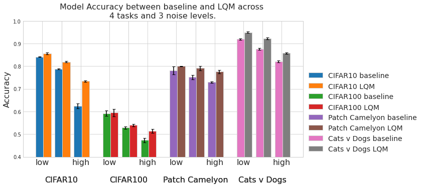
Figure 7: Training with LQM adjusted labels outperforms baselines across all datasets. The improvement from LQM is more prominent in medium and high noise settings. LQM models are trained by stochastically sampling a one-hot label from LQM output distribution, and tuning the $\gamma$ hyperparameter.

Combining LQM with Other Techniques

In the second experiment, we investigate the conjunction of LQM with other noisy labels techniques. We hypothesize that, depending on the technique, LQM may be correcting a different kind of noise from existing techniques, and thus can potentially lead to further performance improvement. To combine LQM with another technique, we sample a hard label from the soft distribution specified by $\tilde{y_{i}}$, and apply other noisy labels techniques on top of the sampled hard label. We consider the same set of noisy labels techniques as the previous section. We find that on CIFAR10 and CIFAR100, combining LQM with other techniques usually lead to further performance improvement. The improvement can also be observed in the high noise setting for CvD. The results are illustrated in Figure 8.

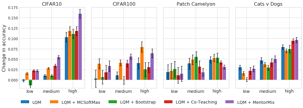
Figure 8: Accuracy improvement of LQM and the combinations of LQM and other techniques compared to the baseline. In many settings (CIFAR10, CIFAR100 and high noise setting in CvD), combining other techniques with LQM further improves the test accuracy. In other cases (PCam and low/medium noise for CvD), the performance gain is less significant.

As a final note, since LQM assumes access to a subset of data with clean labels, and also uses an auxiliary classifier $f(x)$, it has some similarity with semi-supervised learning (SSL). We notice that several state-of-the-art SSL techniques such as FixMatch (Sohn et al., 2020), UDA Xie et al. (2019), self-training with noisy student (Xie et al., 2020) use specifically designed data augmentations that are only suitable for specific types of data, whereas LQM can be applied to any type of data as long as we have rater features. We also expect that combining certain SSL techniques (e.g., data augmentation and consistency training) can further improve the results; however, these extensions are beyond the scope of this paper.

6 Additional Related Work

There is a large body of literature on learning with noisy labels. We mentioned several related work in the previous sections and it is certainly not an exhaustive list. Since we focus on simulation frameworks for noisy label research, we first review prior works that try to simulate noisy labels using methods beyond random label flipping or permutation. As mentioned in previous sections, we are aware that several prior works (Lee et al., 2019; Robinson et al., 2020; Berthon et al., 2021; Zhu et al., 2021; Zhang et al., 2021b) also use similar pseudo-labeling paradigm to generate synthetic datasets with noisy labels. Seo et al. (2019) use a similar idea of nearest neighbor search in the feature space of a pretrained model with clean labels to generate noisy labels. Compared with these works, our study is much more comprehensive with a diverse set of tasks and model architectures. We conduct a series of analysis on the impact of noisy labels, and propose a method to generate synthetic rater features and use them for improving robustness. These points were not considered in the two prior works. Other approaches to simulating label noise have also been studied in the literature. Jiang et al. (2020) proposes a framework to generate controlled web label noise, in which case new images with noisy labels are crawled from the web and then inserted to an existing dataset with clean labels. The framework differs from our approach and the two frameworks should be considered complementary for generating noisy label datasets. In particular, the method by Jiang et al. (2020) is more suitable for web-based data collection, e.g., WebVision (Li et al., 2017a) whereas ours is more suitable for simulating human raters. Moreover, Wang et al. (2018) and Seo et al. (2019) consider open-set noisy labels, where the mislabeled data may not belong to any class of the dataset, similar to Jiang et al. (2020). Another approach to generating datasets with controllable about of label noise is to first identify a dataset with noisy labels (potentially some public datasets (Northcutt et al., 2021a, b)) and then use the confident learning (CL) method (Northcutt et al., 2021a) to increase or decrease the amount of label noise proportionally to the distribution of real-world label noise in the dataset. The idea is to model the joint distribution of noisy and true labels and then generate the noisy labels based on the noise-increased or noise-decreased joint distribution of noisy and true labels. This differs from our method since we use rater models, which are trained neural networks to generate noisy labels for each instance.

Tackling noisy labels using a small subset of data with clean labels has been considered in a few prior works. Common approaches include pretraining or fine-tuning the network using clean labels (Xiao et al., 2015; Krause et al., 2016), and distillation (Li et al., 2017b). In loss correction approaches, a subset of clean labels are often used for estimating the confusion matrix (Patrini et al., 2017; Hendrycks et al., 2018). Veit et al. (2017) propose a method that estimates the residuals between the noisy and clean labels. Ren et al. (2018) use the clean label dataset to learn to reweight the examples. Tsai et al. (2019) combine clean data with self-supervision to learn robust representations. Our approach differs from these prior works since we leverage the additional rater features to learn an auxiliary model that corrects noisy labels in a rater-dependent manner, and can be combined with other techniques to further improve the performance as shown in Section 5. Learning from multiple annotators has been a longstanding research topic. The seminal work by Dawid and Skene (1979) uses the EM algorithm to estimate rater reliability, and much progress has been made since then (Raykar et al., 2010; Zhang et al., 2014; Lakshminarayanan and Teh, 2013). Rater features is commonly available in many human annotation process. In crowdsourcing, several prior work focus on estimating the reliability of raters (Raykar et al., 2010; Tarasov et al., 2014; Moayedikia et al., 2019), and rater aggregation (Vargo et al., 2003; Chen et al., 2013). Item response theory (Embretson and Reise, 2013) from the psychometrics literature uses a latent-trait model to estimate the proficiency of raters and the difficulty of examples, and has a similar underlying principle to our work.

Our method is also broadly related to several other lines of research. Training a pool of rater models is similar to ensemble method (Dietterich, 2000), which is usually used to boost test accuracy (Freund and Schapire, 1997) or improve uncertainty estimation (Lakshminarayanan et al., 2017). Training new models using noisy labels provided by the rater models is similar to knowledge distillation (Buciluǎ et al., 2006; Hinton et al., 2015). Designing instance-dependent noisy label generation framework can be considered as reducing underspecification (D’Amour et al., 2020) in generating label noise.

7 Conclusions and Limitations

In this paper, we propose framework for simulating instance-dependent label noise. Our method is based on the pseudo-labeling paradigm. We show that the distribution of noisy labels in our synthetic datasets is closer to human labels compared to independent random label noise. With our synthetic datasets, we evaluate the negative impact of label noise on deep learning models, and demonstrate that label noise is more detrimental under class imbalanced settings, when pretraining is not used, and on easier tasks. We observe that existing algorithms for learning with noisy labels exhibit different behavior on our synthetic datasets and the datasets with random label noise. Using the rater features from our simulation framework, we propose a new technique, Label Quality Model, that leverages annotator features to predict and correct against noisy labels. We show that our technique can be combined with existing approaches to further improve model performance.

Our work demonstrates the importance of using instance-dependent datasets for noisy label research. As noted above, the performance gain of noisy label techniques on a dataset with independent random label flipping may not directly transfer to our synthetic datasets. We hope our framework can serve as an option for the noisy label research community to develop more efficient methods for practical challenges.

Several limitations of our framework: 1) As discussed in Section 6, it focuses more on simulating human errors, whereas there might be other types of label noise in practical settings that need other simulation methods; 2) Controlling the amount of label noise in the datasets requires careful archtecture selection and hyperparameter tuning, thus is harder compared to random flipping methods; 3) LQM requires the paired-subset containing both clean and noisy labels. This requirement may not be satisfied in some applications.

Appendix

Appendix A Details of Synthetic Datasets

In this section, we provide more details of the synthetic data generation process. In particular, we provide the architectures and hyperparameters of the rater models in these datasets. All the models use standard cosine learning rate decay schedule, as well as the standard flipping and cropping data augmentation. In the following, for rater models that use the same architecture, they are randomly initialized independently.

CIFAR10 datasets in Section 2.3. We use $10$ rater models for the low, medium, and high noise datasets, respectively. Low noise: $3$ Inception-v1 (Szegedy et al., 2015), $1$ Inception-v3 (Szegedy et al., 2016), $2$ Inception-ResNet-v2 (Szegedy et al., 2017), $2$ MobileNet-v1 (Howard et al., 2017), $2$ VGG16 (Simonyan and Zisserman, 2014) models. The models are trained with batch size $256$, $80,000$ steps, and initial learning rate $0.01$. Medium noise: $2$ Inception-v4, $2$ MobileNet-v1, $2$ MobileNet-v2, $1$ NASNetMobile (Zoph et al., 2018), $1$ ResNet50, $1$ ResNet101, $1$ VGG16. All models are trained with batch size $256$, initial learning rate $0.01$ and $17,000$ steps. High noise: $2$ Inception-v2, $1$ Inception-ResNet-v2, $2$ MobileNet-v1, $1$ MobileNet-v2, $2$ ResNet50, $1$ ResNet101, $1$ ResNet152. All models are trained with batch size $256$, initial learning rate $0.01$ and $5,000$ steps.

For the PCam dataset in Section 3.3, we use $20$ rater models involving $10$ architectures: Inception-v1, Inception-v2 (Szegedy et al., 2016), Inception-v3, Inception-v4 (Szegedy et al., 2017), MobileNet-v1, MobileNet-v2 (Sandler et al., 2018), ResNet50, ResNet152 (He et al., 2016), VGG16, VGG19. For each architecture, we use two different initial learning rates: $0.01$ and $0.001$ to train two different models. All the models are trained with batch size $256$ and $10,000$ steps.

For the CvD dataset in Section 3.3, we use $10$ rater models, involving the same $10$ architectures in the PCam dataset mentioned above. All the models are trained with batch size $128$, initial learning rate $0.001$, and $10,000$ steps.

For the Easy task based on CIFAR100 in Section 3.3, we use $10$ rater models with the following architectures: Inception-v1, Inception-v2, Inception-v3, Inception-v4, Inception-ResNet-v2, MobileNet-v1, MobileNet-v2, ResNet50, ResNet101, ResNet152. We use batch size $128$, initial learning rate $3\times 10^{-5}$, and $5,000$ training steps. For the Medium task, we use $11$ rater models, each using its own architecture. The $11$ architectures include the $10$ architectures for the PCam dataset in Section 3.3 with an additional ResNet101. We use batch size $128$, initial learning rate $0.003$, and $40,000$ steps. The Hard task uses $11$ rater models with the same architectures as the Medium task, with batch size $128$, initial learning rate $0.01$ and $2\times 10^{5}$ steps.

For the $3$ CvD datasets in Section 3.1, we use $10$ rater models with the same architectures as the PCam dataset in Section 3.3. All models are trained with batch size $128$. For the three datasets, the (initial learning rate, number of steps) pairs are $(1\times 10^{-2},5\times 10^{4})$, $(1\times 10^{-3},2.5\times 10^{4})$, $(1\times 10^{-3},1\times 10^{5})$, respectively.

For each of the $4$ PCam datasets in Section 3.1, we use $20$ raters models, which uses the same combinations of the $10$ architectures and $2$ initial learning rates as in the PCam dataset in Section 3.3. They all use batch size $256$. The $4$ datasets are generated by varying the number of training steps among $\{1,2,5,8\}\times 10^{4}$.

In Section 3.2, we use $3$ CvD datasets and $3$ CIFAR10 datasets. All the CvD datasets use $10$ rater models with the same set of architectures as the CvD dataset in Section 3.3. All rater models are trained with batch size $128$. The (initial learning rate, number of steps) pairs are $(1\times 10^{-3},1\times 10^{5})$, $(1\times 10^{-3},2.5\times 10^{4})$, $(1\times 10^{-2},1\times 10^{4})$, respectively. The CIFAR10 dataset with rater error rate $0.11$ is the same as the dataset in Section 2.3. The CIFAR10 dataset with rater error rate $0.19$ uses the same rater models as the medium noise dataset in Section 2.3. The CIFAR10 dataset with rater error rate $0.33$ uses the same rater models as the high noise dataset in Section 2.3 with the only difference being that the number of training steps is $12,000$.

In Section 4 and Section 5, we use $3$ datasets for each of the $4$ tasks. The rater error raters of these datasets are provided in the tables in Appendix C. Here, we provide details of the rater models in the synthetic datasets.

CIFAR10 The same as Section 2.3.

CIFAR100 For all the $3$ CIFAR100 datasets, we use $11$ raters, with the same set of architectures as the Medium and Hard tasks in Section 3.3. The (batch size, learning rate, number of steps) tuples for the low, medium, and high noise datasets are $(128,1\times 10^{-3},1\times 10^{4})$, $(256,0.01,2\times 10^{5})$, and $(256,0.01,8\times 10^{4})$, respectively.

PCam For all the $3$ PCam datasets, we use $20$ raters models (for the medium noise dataset, one of the Inception-v1 models failed due to system error, so we only have $19$ noisy labels for this dataset), which uses the same combinations of the $10$ architectures and $2$ initial learning rates as in the PCam dataset in Section 3.3. They all use batch size $256$ and initial learning rate $0.01$. The number of steps are $3.5\times 10^{4}$, $1.5\times 10^{4}$, and $1\times 10^{4}$, for the low, medium, and high noise datasets, respectively.

CvD For all the $3$ CvD datasets, we use $10$ rater models with the same set of architectures as the CvD dataset in Section 3.3. All rater models are trained with batch size $128$. The (initial learning rate, number of steps) pairs are $(1\times 10^{-3},5\times 10^{4})$, $(1\times 10^{-2},1\times 10^{4})$, $(1\times 10^{-3},1\times 10^{4})$, for low, medium, and high noise, respectively.

Appendix B Details for Three CIFAR100-Based Datasets in Section 3.3

As we know, the CIFAR100 dataset contains 20 super classes, each of which contains 5 fine-grained classes. We create the easy, medium, and hard tasks in the following way.

• For the easy task, we select one fine-grained class from each of the 20 super classes, and form a 20-way classification task.

• For the medium task, we select 4 super classes that are semantically similar, i.e., large carnivores, large omnivores and herbivores, small mammals, and medium-sized mammals. We use all the fine-grained classes from these 4 super classes to form a 20-way classification task.

• For the hard task, we simply classify the 20 super classes, and we randomly subsample the data in order to match the total number of data points in the other two tasks. We note that this task is harder since the data in each super class is a mixture of 5 fine-grained classes.

Appendix C Benchmarking Results

We provide exact numbers for the experimental results in Section 4 (Tables 2, 3, 4, and 5) and Section 5 in the main paper (Tables 6, 7, 8, and 9).

Table 2: Test accuracy $\pm$ std (%) of noisy label algorithms on CIFAR10

noise	low (err=0.11)		medium (err=0.19)		high (err=0.48)
dataset	synthetic	random	synthetic	random	synthetic	random
Baseline	83.6 $\pm$ 0.5	78.7 $\pm$ 0.3	78.4 $\pm$ 0.1	72.9 $\pm$ 0.7	60.1 $\pm$ 0.2	61.9 $\pm$ 0.6
Bootstrap	83.2 $\pm$ 0.8	78.8 $\pm$ 0.6	77.6 $\pm$ 0.1	74.8 $\pm$ 0.7	61.5 $\pm$ 1.2	63.5 $\pm$ 0.7
Co-Teaching	85.9 $\pm$ 0.2	87.2 $\pm$ 0.6	81.6 $\pm$ 0.5	86.2 $\pm$ 0.2	63.4 $\pm$ 1.6	66.1 $\pm$ 0.9
MCSoftMax	85.9 $\pm$ 0.1	82.2 $\pm$ 0.3	79.8 $\pm$ 0.2	75.5 $\pm$ 1.1	65.2 $\pm$ 0.4	60.4 $\pm$ 0.8
MentorMix	85.5 $\pm$ 1.9	87.7 $\pm$ 0.2	83.4 $\pm$ 0.7	86.9 $\pm$ 0.3	69.4 $\pm$ 1.5	78.9 $\pm$ 0.9

Table 3: Test accuracy $\pm$ std (%) of noisy label algorithms on CIFAR100

noise	low (err=0.25)		medium (err=0.38)		high (err=0.43)
dataset	synthetic	random	synthetic	random	synthetic	random
Baseline	58.8 $\pm$ 0.5	42.3 $\pm$ 0.3	51.1 $\pm$ 0.5	34.4 $\pm$ 1.1	46.7 $\pm$ 1.2	29.9 $\pm$ 0.6
Bootstrap	58.4 $\pm$ 0.6	43.3 $\pm$ 0.3	51.5 $\pm$ 0.8	35.9 $\pm$ 0.9	46.6 $\pm$ 0.9	29.6 $\pm$ 0.7
Co-Teaching	60.1 $\pm$ 0.6	55.2 $\pm$ 0.7	52.7 $\pm$ 0.5	44.6 $\pm$ 1.2	49.2 $\pm$ 1.2	39.2 $\pm$ 1.4
MCSoftMax	60.7 $\pm$ 0.4	47.8 $\pm$ 0.5	53.0 $\pm$ 0.4	41.2 $\pm$ 1.2	48.5 $\pm$ 0.3	38.8 $\pm$ 0.8
MentorMix	62.2 $\pm$ 0.1	59.6 $\pm$ 0.6	56.4 $\pm$ 0.3	53.9 $\pm$ 0.4	50.0 $\pm$ 0.8	49.0 $\pm$ 0.5

Table 4: Test accuracy $\pm$ std (%) of noisy label algorithms on PatchCamelyon

noise	low (err=0.10)		medium (err=0.18)		high (err=0.23)
dataset	synthetic	random	synthetic	random	synthetic	random
Baseline	82.1 $\pm$ 1.3	82.6 $\pm$ 1.0	78.9 $\pm$ 0.2	82.2 $\pm$ 1.0	75.7 $\pm$ 0.7	81.6 $\pm$ 0.6
Bootstrap	82.9 $\pm$ 1.4	82.8 $\pm$ 1.6	78.6 $\pm$ 0.9	81.4 $\pm$ 0.5	76.4 $\pm$ 0.7	80.3 $\pm$ 1.3
Co-Teaching	82.0 $\pm$ 0.8	82.7 $\pm$ 0.6	80.1 $\pm$ 1.4	81.4 $\pm$ 1.2	77.5 $\pm$ 1.5	80.9 $\pm$ 0.8
MCSoftMax	81.9 $\pm$ 1.5	83.4 $\pm$ 1.6	79.4 $\pm$ 1.2	83.7 $\pm$ 0.5	72.3 $\pm$ 6.7	82.3 $\pm$ 1.8
MentorMix	83.2 $\pm$ 1.1	81.7 $\pm$ 0.6	76.2 $\pm$ 1.9	83.0 $\pm$ 0.3	73.6 $\pm$ 1.6	79.7 $\pm$ 1.0

Table 5: Test accuracy $\pm$ std (%) of noisy label algorithms on Cats vs Dogs

noise	low (err=0.09)		medium (err=0.20)		high (err=0.29)
dataset	synthetic	random	synthetic	random	synthetic	random
Baseline	92.0 $\pm$ 0.4	92.3 $\pm$ 0.2	85.4 $\pm$ 0.7	88.8 $\pm$ 0.5	82.0 $\pm$ 0.7	82.7 $\pm$ 2.1
Bootstrap	92.1 $\pm$ 0.6	93.8 $\pm$ 0.6	87.3 $\pm$ 1.0	89.0 $\pm$ 0.8	82.4 $\pm$ 0.6	85.8 $\pm$ 0.4
Co-Teaching	93.4 $\pm$ 0.2	96.2 $\pm$ 0.2	89.7 $\pm$ 0.5	92.6 $\pm$ 0.2	84.0 $\pm$ 0.6	86.7 $\pm$ 1.3
MCSoftMax	92.0 $\pm$ 0.3	93.7 $\pm$ 0.3	87.6 $\pm$ 0.5	90.4 $\pm$ 0.5	81.2 $\pm$ 0.4	85.1 $\pm$ 1.2
MentorMix	94.0 $\pm$ 0.6	94.2 $\pm$ 0.4	90.0 $\pm$ 0.7	92.0 $\pm$ 0.4	84.8 $\pm$ 0.6	89.6 $\pm$ 0.8

Table 6: Training with LQM outputs with various techniques. Test accuracy $\pm$ std (%) on CIFAR10

algorithm	low (err=0.11)	medium (err=0.19)	high (err=0.48)
Baseline	84.1 $\pm$ 0.2	78.8 $\pm$ 0.2	62.4 $\pm$ 1.1
LQM	85.6 $\pm$ 0.4	81.9 $\pm$ 0.3	73.4 $\pm$ 0.3
LQM + Bootstrap	82.8 $\pm$ 0.9	79.8 $\pm$ 0.2	73.5 $\pm$ 0.3
LQM + Co-Teaching	86.3 $\pm$ 0.2	80.9 $\pm$ 0.1	74.2 $\pm$ 0.4
LQM + MCSoftMax	85.7 $\pm$ 0.2	81.6 $\pm$ 0.1	74.2 $\pm$ 0.2
LQM + MentorMix	86.3 $\pm$ 0.1	84.2 $\pm$ 0.3	78.4 $\pm$ 0.2

Table 7: Training with LQM outputs with various techniques. Test accuracy $\pm$ std (%) on CIFAR100

algorithm	low (err=0.25)	medium (err=0.38)	high (err=0.43)
Baseline	59.2 $\pm$ 1.2	52.9 $\pm$ 0.6	47.3 $\pm$ 1.0
LQM	59.4 $\pm$ 1.7	53.9 $\pm$ 0.6	51.3 $\pm$ 0.9
LQM + Bootstrap	59.8 $\pm$ 1.1	52.8 $\pm$ 0.8	49.8 $\pm$ 1.4
LQM + Co-Teaching	61.0 $\pm$ 1.3	56.8 $\pm$ 0.6	50.4 $\pm$ 0.7
LQM + MCSoftMax	63.0 $\pm$ 0.2	57.0 $\pm$ 0.4	55.2 $\pm$ 0.7
LQM + MentorMix	62.4 $\pm$ 0.5	58.5 $\pm$ 0.2	53.7 $\pm$ 0.4

Table 8: Training with LQM outputs with various techniques. Test accuracy $\pm$ std (%) on PatchCamelyon

algorithm	low (err=0.1)	medium (err=0.18)	high (err=0.23)
Baseline	78.1 $\pm$ 1.8	75.1 $\pm$ 0.9	72.9 $\pm$ 0.3
LQM	80.0 $\pm$ 0.1	79.1 $\pm$ 0.9	77.6 $\pm$ 0.7
LQM + Bootstrap	80.7 $\pm$ 0.7	80.7 $\pm$ 0.9	78.2 $\pm$ 1.1
LQM + Co-Teaching	78.9 $\pm$ 0.1	78.2 $\pm$ 1.7	76.9 $\pm$ 0.3
LQM + MCSoftMax	80.3 $\pm$ 0.4	80.0 $\pm$ 0.7	78.2 $\pm$ 0.9
LQM + MentorMix	79.5 $\pm$ 0.5	77.0 $\pm$ 0.4	75.8 $\pm$ 0.2

Table 9: Training with LQM outputs with various techniques. Test accuracy $\pm$ std (%) on Cats vs Dogs

algorithm	low (err=0.09)	medium (err=0.20)	high (err=0.29)
Baseline	91.9 $\pm$ 0.3	87.6 $\pm$ 0.5	82.0 $\pm$ 0.5
LQM	94.9 $\pm$ 0.4	92.3 $\pm$ 0.4	85.8 $\pm$ 0.4
LQM + Bootstrap	92.0 $\pm$ 0.4	90.5 $\pm$ 0.3	89.5 $\pm$ 0.8
LQM + Co-Teaching	94.1 $\pm$ 0.8	91.5 $\pm$ 0.5	90.9 $\pm$ 0.5
LQM + MCSoftMax	93.5 $\pm$ 0.2	91.3 $\pm$ 0.2	89.1 $\pm$ 0.1
LQM + MentorMix	94.6 $\pm$ 0.6	92.1 $\pm$ 0.5	91.1 $\pm$ 0.3

References

- Advani et al. (2020) M. S. Advani, A. M. Saxe, and H. Sompolinsky. High-dimensional dynamics of generalization error in neural networks. Neural Networks, 132:428–446, 2020.
- Angluin and Laird (1988) D. Angluin and P. Laird. Learning from noisy examples. Machine Learning, 2(4):343–370, 1988.
- Bejnordi et al. (2017) B. E. Bejnordi, M. Veta, P. J. Van Diest, B. Van Ginneken, N. Karssemeijer, G. Litjens, J. A. Van Der Laak, M. Hermsen, Q. F. Manson, M. Balkenhol, et al. Diagnostic assessment of deep learning algorithms for detection of lymph node metastases in women with breast cancer. Jama, 318(22):2199–2210, 2017.
- Belkin et al. (2019) M. Belkin, D. Hsu, S. Ma, and S. Mandal. Reconciling modern machine-learning practice and the classical bias–variance trade-off. Proceedings of the National Academy of Sciences, 116(32):15849–15854, 2019.
- Berthon et al. (2021) A. Berthon, B. Han, G. Niu, T. Liu, and M. Sugiyama. Confidence scores make instance-dependent label-noise learning possible. In International Conference on Machine Learning, pages 825–836. PMLR, 2021.
- Borkan et al. (2019) D. Borkan, L. Dixon, J. Sorensen, N. Thain, and L. Vasserman. Nuanced metrics for measuring unintended bias with real data for text classification. In Companion Proceedings of the 2019 World Wide Web Conference, pages 491–500, 2019.
- Buciluǎ et al. (2006) C. Buciluǎ, R. Caruana, and A. Niculescu-Mizil. Model compression. In Proceedings of the 12th ACM SIGKDD International Conference on Knowledge Discovery and Data Mining, pages 535–541, 2006.
- Cabitza et al. (2020) F. Cabitza, A. Campagner, D. Albano, A. Aliprandi, A. Bruno, V. Chianca, A. Corazza, F. Di Pietto, A. Gambino, S. Gitto, et al. The elephant in the machine: Proposing a new metric of data reliability and its application to a medical case to assess classification reliability. Applied Sciences, 10(11):4014, 2020.
- Chapelle et al. (2006) O. Chapelle, B. Schölkopf, and A. Zien. Semi-Supervised Learning. The MIT Press, 2006.
- Chen et al. (2013) X. Chen, P. N. Bennett, K. Collins-Thompson, and E. Horvitz. Pairwise ranking aggregation in a crowdsourced setting. In Proceedings of the sixth ACM International Conference on Web Search and Data Mining, pages 193–202, 2013.
- Collier et al. (2020) M. Collier, B. Mustafa, E. Kokiopoulou, R. Jenatton, and J. Berent. A simple probabilistic method for deep classification under input-dependent label noise. arXiv preprint arXiv:2003.06778, 2020.
- D’Amour et al. (2020) A. D’Amour, K. Heller, D. Moldovan, B. Adlam, B. Alipanahi, A. Beutel, C. Chen, J. Deaton, J. Eisenstein, M. D. Hoffman, et al. Underspecification presents challenges for credibility in modern machine learning. arXiv preprint arXiv:2011.03395, 2020.
- Dawid and Skene (1979) A. P. Dawid and A. M. Skene. Maximum likelihood estimation of observer error-rates using the EM algorithm. Journal of the Royal Statistical Society: Series C (Applied Statistics), 28(1):20–28, 1979.
- Deng et al. (2009) J. Deng, W. Dong, R. Socher, L.-J. Li, K. Li, and L. Fei-Fei. ImageNet: A large-scale hierarchical image database. In 2009 IEEE Conference on Computer Vision and Pattern Recognition, pages 248–255. IEEE, 2009.
- Dietterich (2000) T. G. Dietterich. Ensemble methods in machine learning. In International Workshop on Multiple Classifier Systems, pages 1–15. Springer, 2000.
- Elson et al. (2007) J. Elson, J. R. Douceur, J. Howell, and J. Saul. Asirra: a CAPTCHA that exploits interest-aligned manual image categorization. In ACM Conference on Computer and Communications Security, volume 7, pages 366–374, 2007.
- Embretson and Reise (2013) S. E. Embretson and S. P. Reise. Item response theory. Psychology Press, 2013.
- Freund and Schapire (1997) Y. Freund and R. E. Schapire. A decision-theoretic generalization of on-line learning and an application to boosting. Journal of Computer and System Sciences, 55(1):119–139, 1997.
- Han et al. (2018) B. Han, Q. Yao, X. Yu, G. Niu, M. Xu, W. Hu, I. Tsang, and M. Sugiyama. Co-Teaching: Robust training of deep neural networks with extremely noisy labels. arXiv preprint arXiv:1804.06872, 2018.
- Hayes and Krippendorff (2007) A. F. Hayes and K. Krippendorff. Answering the call for a standard reliability measure for coding data. Communication Methods and Measures, 1(1):77–89, 2007.
- He et al. (2016) K. He, X. Zhang, S. Ren, and J. Sun. Deep residual learning for image recognition. In Proceedings of the IEEE Conference on Computer Vision and Pattern Recognition, pages 770–778, 2016.
- Hendrycks et al. (2018) D. Hendrycks, M. Mazeika, D. Wilson, and K. Gimpel. Using trusted data to train deep networks on labels corrupted by severe noise. arXiv preprint arXiv:1802.05300, 2018.
- Hendrycks et al. (2019) D. Hendrycks, K. Lee, and M. Mazeika. Using pre-training can improve model robustness and uncertainty. In International Conference on Machine Learning, pages 2712–2721. PMLR, 2019.
- Hinton et al. (2015) G. Hinton, O. Vinyals, and J. Dean. Distilling the knowledge in a neural network. arXiv preprint arXiv:1503.02531, 2015.
- Howard et al. (2017) A. G. Howard, M. Zhu, B. Chen, D. Kalenichenko, W. Wang, T. Weyand, M. Andreetto, and H. Adam. MobileNets: Efficient convolutional neural networks for mobile vision applications. arXiv preprint arXiv:1704.04861, 2017.
- Jiang et al. (2018) L. Jiang, Z. Zhou, T. Leung, L.-J. Li, and L. Fei-Fei. MentorNet: Learning data-driven curriculum for very deep neural networks on corrupted labels. In International Conference on Machine Learning, pages 2304–2313. PMLR, 2018.
- Jiang et al. (2020) L. Jiang, D. Huang, M. Liu, and W. Yang. Beyond synthetic noise: Deep learning on controlled noisy labels. In International Conference on Machine Learning, pages 4804–4815. PMLR, 2020.
- Khetan et al. (2017) A. Khetan, Z. C. Lipton, and A. Anandkumar. Learning from noisy singly-labeled data. arXiv preprint arXiv:1712.04577, 2017.
- Krause et al. (2016) J. Krause, B. Sapp, A. Howard, H. Zhou, A. Toshev, T. Duerig, J. Philbin, and L. Fei-Fei. The unreasonable effectiveness of noisy data for fine-grained recognition. In European Conference on Computer Vision, pages 301–320. Springer, 2016.
- Krizhevsky and Hinton (2009) A. Krizhevsky and G. Hinton. Learning multiple layers of features from tiny images. Technical Report, 2009.
- Lakshminarayanan and Teh (2013) B. Lakshminarayanan and Y. W. Teh. Inferring ground truth from multi-annotator ordinal data: a probabilistic approach. arXiv preprint arXiv:1305.0015, 2013.
- Lakshminarayanan et al. (2017) B. Lakshminarayanan, A. Pritzel, and C. Blundell. Simple and scalable predictive uncertainty estimation using deep ensembles. Advances in Neural Information Processing Systems, 30, 2017.
- Lee et al. (2019) K. Lee, S. Yun, K. Lee, H. Lee, B. Li, and J. Shin. Robust inference via generative classifiers for handling noisy labels. In International Conference on Machine Learning, pages 3763–3772. PMLR, 2019.
- Lee et al. (2018) K.-H. Lee, X. He, L. Zhang, and L. Yang. CleanNet: Transfer learning for scalable image classifier training with label noise. In Proceedings of the IEEE Conference on Computer Vision and Pattern Recognition, pages 5447–5456, 2018.
- Li et al. (2020a) J. Li, R. Socher, and S. C. Hoi. DivideMix: Learning with noisy labels as semi-supervised learning. arXiv preprint arXiv:2002.07394, 2020a.
- Li et al. (2020b) M. Li, M. Soltanolkotabi, and S. Oymak. Gradient descent with early stopping is provably robust to label noise for overparameterized neural networks. In International Conference on Artificial Intelligence and Statistics, pages 4313–4324. PMLR, 2020b.
- Li et al. (2017a) W. Li, L. Wang, W. Li, E. Agustsson, and L. Van Gool. WebVision database: Visual learning and understanding from web data. arXiv preprint arXiv:1708.02862, 2017a.
- Li et al. (2017b) Y. Li, J. Yang, Y. Song, L. Cao, J. Luo, and L.-J. Li. Learning from noisy labels with distillation. In Proceedings of the IEEE International Conference on Computer Vision, pages 1910–1918, 2017b.
- Malach and Shalev-Shwartz (2017) E. Malach and S. Shalev-Shwartz. Decoupling “when to update” from “how to update”. arXiv preprint arXiv:1706.02613, 2017.
- Moayedikia et al. (2019) A. Moayedikia, W. Yeoh, K.-L. Ong, and Y. L. Boo. Improving accuracy and lowering cost in crowdsourcing through an unsupervised expertise estimation approach. Decision Support Systems, 122:113065, 2019.
- Natarajan et al. (2013) N. Natarajan, I. S. Dhillon, P. Ravikumar, and A. Tewari. Learning with noisy labels. In Neural Information Processing Systems, volume 26, pages 1196–1204, 2013.
- Northcutt et al. (2021a) C. Northcutt, L. Jiang, and I. Chuang. Confident learning: Estimating uncertainty in dataset labels. Journal of Artificial Intelligence Research, 70:1373–1411, 2021a.
- Northcutt et al. (2021b) C. G. Northcutt, A. Athalye, and J. Mueller. Pervasive label errors in test sets destabilize machine learning benchmarks. arXiv preprint arXiv:2103.14749, 2021b.
- Patrini et al. (2017) G. Patrini, A. Rozza, A. Krishna Menon, R. Nock, and L. Qu. Making deep neural networks robust to label noise: A loss correction approach. In Proceedings of the IEEE Conference on Computer Vision and Pattern Recognition, pages 1944–1952, 2017.
- Peterson et al. (2019) J. C. Peterson, R. M. Battleday, T. L. Griffiths, and O. Russakovsky. Human uncertainty makes classification more robust. In Proceedings of the IEEE/CVF International Conference on Computer Vision, pages 9617–9626, 2019.
- Raghavan et al. (1989) V. Raghavan, P. Bollmann, and G. S. Jung. A critical investigation of recall and precision as measures of retrieval system performance. ACM Transactions on Information Systems (TOIS), 7(3):205–229, 1989.
- Ratner et al. (2016) A. Ratner, C. De Sa, S. Wu, D. Selsam, and C. Ré. Data programming: Creating large training sets, quickly. Advances in Neural Information Processing Systems, 29:3567, 2016.
- Ratner et al. (2017) A. Ratner, S. H. Bach, H. Ehrenberg, J. Fries, S. Wu, and C. Ré. Snorkel: Rapid training data creation with weak supervision. In Proceedings of the VLDB Endowment. International Conference on Very Large Data Bases, volume 11, page 269. NIH Public Access, 2017.
- Raykar et al. (2010) V. C. Raykar, S. Yu, L. H. Zhao, G. H. Valadez, C. Florin, L. Bogoni, and L. Moy. Learning from crowds. Journal of Machine Learning Research, 11(4), 2010.
- Reed et al. (2014) S. Reed, H. Lee, D. Anguelov, C. Szegedy, D. Erhan, and A. Rabinovich. Training deep neural networks on noisy labels with bootstrapping. arXiv preprint arXiv:1412.6596, 2014.
- Ren et al. (2018) M. Ren, W. Zeng, B. Yang, and R. Urtasun. Learning to reweight examples for robust deep learning. In International Conference on Machine Learning, pages 4334–4343. PMLR, 2018.
- Robinson et al. (2020) J. Robinson, S. Jegelka, and S. Sra. Strength from weakness: Fast learning using weak supervision. In International Conference on Machine Learning, pages 8127–8136. PMLR, 2020.
- Rolnick et al. (2017) D. Rolnick, A. Veit, S. Belongie, and N. Shavit. Deep learning is robust to massive label noise. arXiv preprint arXiv:1705.10694, 2017.
- Sandler et al. (2018) M. Sandler, A. Howard, M. Zhu, A. Zhmoginov, and L.-C. Chen. MobileNetv2: Inverted residuals and linear bottlenecks. In Proceedings of the IEEE Conference on Computer Vision and Pattern Recognition, pages 4510–4520, 2018.
- Seo et al. (2019) P. H. Seo, G. Kim, and B. Han. Combinatorial inference against label noise. In Advances in Neural Information Processing Systems, volume 32, 2019.
- Simonyan and Zisserman (2014) K. Simonyan and A. Zisserman. Very deep convolutional networks for large-scale image recognition. arXiv preprint arXiv:1409.1556, 2014.
- Sohn et al. (2020) K. Sohn, D. Berthelot, C.-L. Li, Z. Zhang, N. Carlini, E. D. Cubuk, A. Kurakin, H. Zhang, and C. Raffel. FixMatch: Simplifying semi-supervised learning with consistency and confidence. arXiv preprint arXiv:2001.07685, 2020.
- Szegedy et al. (2015) C. Szegedy, W. Liu, Y. Jia, P. Sermanet, S. Reed, D. Anguelov, D. Erhan, V. Vanhoucke, and A. Rabinovich. Going deeper with convolutions. In Proceedings of the IEEE Conference on Computer Vision and Pattern Recognition, pages 1–9, 2015.
- Szegedy et al. (2016) C. Szegedy, V. Vanhoucke, S. Ioffe, J. Shlens, and Z. Wojna. Rethinking the inception architecture for computer vision. In Proceedings of the IEEE Conference on Computer Vision and Pattern Recognition, pages 2818–2826, 2016.
- Szegedy et al. (2017) C. Szegedy, S. Ioffe, V. Vanhoucke, and A. Alemi. Inception-v4, Inception-Resnet and the impact of residual connections on learning. In Proceedings of the AAAI Conference on Artificial Intelligence, volume 31, 2017.
- Tarasov et al. (2014) A. Tarasov, S. J. Delany, and B. Mac Namee. Dynamic estimation of worker reliability in crowdsourcing for regression tasks: Making it work. Expert Systems with Applications, 41(14):6190–6210, 2014.
- Tsai et al. (2019) T. W. Tsai, C. Li, and J. Zhu. Countering noisy labels by learning from auxiliary clean labels. arXiv preprint arXiv:1905.13305, 2019.
- Vargo et al. (2003) J. Vargo, J. C. Nesbit, K. Belfer, and A. Archambault. Learning object evaluation: computer-mediated collaboration and inter-rater reliability. International Journal of Computers and Applications, 25(3):198–205, 2003.
- Veeling et al. (2018) B. S. Veeling, J. Linmans, J. Winkens, T. Cohen, and M. Welling. Rotation equivariant CNNs for digital pathology. In International Conference on Medical image computing and computer-assisted intervention, pages 210–218. Springer, 2018.
- Veit et al. (2017) A. Veit, N. Alldrin, G. Chechik, I. Krasin, A. Gupta, and S. Belongie. Learning from noisy large-scale datasets with minimal supervision. In Proceedings of the IEEE Conference on Computer Vision and Pattern Recognition, pages 839–847, 2017.
- Wang et al. (2018) Y. Wang, W. Liu, X. Ma, J. Bailey, H. Zha, L. Song, and S.-T. Xia. Iterative learning with open-set noisy labels. In Proceedings of the IEEE Conference on Computer Vision and Pattern Recognition, pages 8688–8696, 2018.
- Wang et al. (2019) Y. Wang, X. Ma, Z. Chen, Y. Luo, J. Yi, and J. Bailey. Symmetric cross entropy for robust learning with noisy labels. In Proceedings of the IEEE/CVF International Conference on Computer Vision, pages 322–330, 2019.
- Xiao et al. (2015) T. Xiao, T. Xia, Y. Yang, C. Huang, and X. Wang. Learning from massive noisy labeled data for image classification. In Proceedings of the IEEE Conference on Computer Vision and Pattern Recognition, pages 2691–2699, 2015.
- Xie et al. (2019) Q. Xie, Z. Dai, E. Hovy, M.-T. Luong, and Q. V. Le. Unsupervised data augmentation for consistency training. arXiv preprint arXiv:1904.12848, 2019.
- Xie et al. (2020) Q. Xie, M.-T. Luong, E. Hovy, and Q. V. Le. Self-training with noisy student improves ImageNet classification. In Proceedings of the IEEE/CVF Conference on Computer Vision and Pattern Recognition, pages 10687–10698, 2020.
- Zhang et al. (2021a) C. Zhang, S. Bengio, M. Hardt, B. Recht, and O. Vinyals. Understanding deep learning (still) requires rethinking generalization. Communications of the ACM, 64(3):107–115, 2021a.
- Zhang and Zhang (2009) E. Zhang and Y. Zhang. Average precision. Encyclopedia of Database Systems, pages 192–193, 2009.
- Zhang et al. (2017) H. Zhang, M. Cisse, Y. N. Dauphin, and D. Lopez-Paz. mixup: Beyond empirical risk minimization. arXiv preprint arXiv:1710.09412, 2017.
- Zhang et al. (2014) Y. Zhang, X. Chen, D. Zhou, and M. I. Jordan. Spectral methods meet EM: A provably optimal algorithm for crowdsourcing. Advances in Neural Information Processing Systems, 27:1260–1268, 2014.
- Zhang et al. (2021b) Y. Zhang, S. Zheng, P. Wu, M. Goswami, and C. Chen. Learning with feature-dependent label noise: A progressive approach. arXiv preprint arXiv:2103.07756, 2021b.
- Zhu et al. (2021) Z. Zhu, T. Liu, and Y. Liu. A second-order approach to learning with instance-dependent label noise. In Proceedings of the IEEE/CVF Conference on Computer Vision and Pattern Recognition, pages 10113–10123, 2021.
- Zoph et al. (2018) B. Zoph, V. Vasudevan, J. Shlens, and Q. V. Le. Learning transferable architectures for scalable image recognition. In Proceedings of the IEEE Conference on Computer Vision and Pattern Recognition, pages 8697–8710, 2018.