Surface-induced reduction of the switching field in nanomagnets
Abstract
Magnetization reversal in a many-spin nanomagnet subjected to an rf magnetic field, on top of a DC magnetic field, is studied by numerically solving the system of coupled (damped) Landau-Lifshitz equations. It is demonstrated that spin-misalignment induced by surface anisotropy favors switching with a DC magnetic field weaker than the Stoner-Wohlfarth switching field, for optimal intensities and frequencies of the rf field.
I introduction
Storing data on magnetic media involves magnetization reversal between two magnetic states, the and states. In recent years, in order to optimize magnetic recording, a variety of nanoscale magnetic systems has been extensively investigated. However, the two magnetic states in such systems are usually separated by high magnetic anisotropy energy barriers. While this is favorable to thermal stability of the data stored, high magnetic fields are required for their switching (and thus for writing and reading). The problem is that these fields are rather difficult to achieve at the nanoscale because of heating and noise issues, for instance. As such, several strategies have been attempted to overcome such a hurdle, and one of which consists in applying a time-dependent magnetic (rf) field. This has been shown to considerably reduce the static switching field (the Stoner-Wohlfarth switching field), see e.g. Refs. (C. Thirion, W. Wernsdorfer and D. Mailly, Switching of magnetization by nonlinear resonance studied in single nanoparticles, 2003; Woltersdorf et al., 2007; N. Barros, M. Rassam, H. Jirari and H. Kachkachi, Optimal switching of a nanomagnet assisted by microwaves, 2011; N. Barros, M. Rassam and H. Kachkachi, Microwave-assisted switching of a nanomagnet: Analytical determination of the optimal microwave field, 2013; Suto et al., 2017) and many references therein. Several works (Sun and Wang, 2006; N. Barros, M. Rassam and H. Kachkachi, Microwave-assisted switching of a nanomagnet: Analytical determination of the optimal microwave field, 2013; Cai et al., 2013; Taniguchi et al., 2016) have proceeded by applying an rf field and solving the Landau-Lifshitz equation in the macrospin approach. Alternatively, it was shown in Refs. (D. A. Garanin, H. Kachkachi and L. Reynaud, Magnetization reversal and nonexponential relaxation via instabilities of internal spin waves in nanomagnets, 2008; D. A. Garanin and H. Kachkachi, Magnetization reversal via internal spin waves in magnetic nanoparticles, 2009) that the magnetization switching in nanomagnets in the many-spin approach may be achieved via internal second-generation spin-wave modes. Recent experimental and theoretical studies (Seki et al., 2023; Yamaji and Imamura, 2016) have also investigated switching assisted by spin waves and have showed that these lead to a reduction of the switching field.
In general, the generation of spin waves is triggered by spin misalignment and, in nanomagnets, the latter is most often caused by boundary effects and surface anisotropy. Accordingly, in the present work, we investigate how surface anisotropy affects switching and, in particular, how the switching field intensity and frequency depend on surface anisotropy and the size of the nanomagnet. For this purpose, we consider the simplest nanomagnet of cubic shape, an underlying simple cubic lattice structure, and a typical set of energy parameters such as exchange coupling, core and surface anisotropy constants (H. Kachkachi and D.A. Garanin, 2005; Schmool and Kachkachi, 2015, 2016; Kanso et al., 2019; Iglesias and Kachkachi, 2021). We consider a nanomagnet of classical (atomic) magnetic moments , with a unit vector and the amplitude. The magnetic properties of such a nanomagnet may be investigated with the help of the Dirac-Heisenberg Hamiltonian(D.A. Dimitrov and Wysin, Effects of surface anisotropy on hysteresis in fine magnetic particles, 1994; O. Iglesias and A. Labarta, Finite-size and surface effects in maghemite nanoparticles: Monte Carlo simulations, 2001; H. Kachkachi and M. Dimian, Hysteretic properties of a magnetic particle with strong surface anisotropy, 2002; N. Kazantseva, D. Hinzke, U. Nowak, R. W. Chantrell, U. Atxitia, and O. Chubykalo-Fesenko, Towards multiscale modeling of magnetic materials: Simulations of FePt, 2008; Fraile Rodríguez et al., 2010; R. Bastardis, U. Atxitia, O. Chubykalo-Fesenko, and H. Kachkachi, Unified decoupling scheme for exchange and anisotropy contributions and temperature-dependent spectral properties of anisotropic spin systems, 2012)
| (1) |
where the first term is the exchange energy with coupling . In general, one may introduce an exchange coupling that depends on the loci of the spins. However, for the present study and the message it aims to deliver, it is sufficient to consider a uniform exchange coupling throughout the nanomagnet and use it as a reference energy scale for the whole study, which means that all other parameters are measured with respect to . In the second term in Eq. (1), which is the Zeeman coupling energy, we introduced the reduced magnetic field
| (2) |
comprising the static (or DC) magnetic field and the time-dependent rf field . The latter is taken circularly polarized in the plane (S. I. Denisov, T.V. Lyutyy, and P. Hänggi, Magnetization of nanoparticle systems in a rotating magnetic field, 2006)
| (3) |
where is the dimensionless time measured with respect to the characteristic scaling time of the system’s dynamics, namely , being the gyromagnetic ratio (); is the dimensionless frequency.
The last term in Eq. (1) is the anisotropy energy contribution with being the on-site anisotropy energy. Here, we distinguish between core and surface spins according to whether they have their full coordination number (here ) or not. Indeed, the nanomagnet under study is a box-shaped many-spin system with free boundary conditions, with an underlying simple-cubic lattice. Therefore, there are five different local environments with a coordination number corresponding respectively to the core (), facets (), edges () and corners (). Then, to core spins we attribute a uniaxial (on-site) anisotropy with easy axis along the direction and constant . On the other hand, the anisotropy of surface spins is given by Néel’s model (L. Néel, Anisotropie magnétique superficielle et surstructures d’orientation, 1954), according to which anisotropy only occurs at sites with reduced coordination. The corresponding anisotropy constant is denoted by . Therefore, we write
| (4) |
is a unit vector connecting the nearest neighbors (nn) and .
Physical parameters: A word is in order regarding the orders of magnitude of these parameters. For cobalt, the lattice parameter is nm and the magnetic moment per atom is , with being the number of Bohr magnetons per atom () and J/T the Bohr magneton. Hence, . The (bulk) exchange coupling is or J/atom, which yields . Next, the magneto-crystalline anisotropy constant is roughly J/atom and the surface anisotropy constant is Joule/atom. As such, and . The latter value is within the range of those inferred from several experimental studies. Indeed, one may find for cobalt (R. Skomski and J.M.D. Coey, 1999), for iron (K.B. Urquhart, B. Heinrich, J.F. Cochran, A.S. Arrott, and K. Myrtle, Ferromagnetic resonance in ultrahigh vacuum of bcc Fe films grown on Ag(001)(1988), 001), and for maghemite particles (R. Perzynski and Yu.L. Raikher, 2005). For later reference, we note that for a nanomagnet with the atomic magnetic moment and magneto-crystalline anisotropy given above, the Stoner-Wohlfarth switching field evaluates to .
Another word is in order regarding the notations for the anisotropy constants. The capital letter stands for the macroscopic constant usually given in for the volume and for the surface. It can also be converted into upon using the unit cell of the underlying lattice. The lowercase letter is the dimensionless anisotropy constant that results from a normalization with respect to the largest energy in the system, namely the exchange coupling , i.e. , for core and surface. In the figures presented below, instead of using the dimensionless constant , we use the anisotropy constant in units of which should be understood as .
The dynamics of the atomic spins is described with a set of () coupled damped Landau-Lifshitz equations (LLE)
| (5) |
where is the (dimensionless) effective field acting on the atomic spin at site , given by ; is the dimensionless damping parameter ().
We use the (second-order) Heun algorithm to solve the set of equations (5) starting from a given initial state (a configuration of spins ) and a set of parameters and rf field characteristics, i.e. amplitude and frequency . The calculations will be performed for two anisotropy configurations:
-
1.
Model TUA (textured uniaxial anisotropy): all spins, core and surface, have the same uniaxial anisotropy in the direction, but the corresponding constant may be different for core and surface spins.
-
2.
Model NSA (Néel surface anisotropy): the spins in the core are attributed the uniaxial anisotropy easy axis according to the first line in Eq. (4) with constant and easy axis , whereas those on the surface have their anisotropy given by the second line with constant .
In this study we vary the amplitude and frequency of the rf field and determine their optimal values for which the net magnetic moment switches, for a given and fixed DC magnetic field.
Numerical procedure: we recall that the main objective here is to achieve magnetization reversal under an rf field, in addition to a DC magnetic field whose intensity is supposedly smaller than the critical value required for switching according to the macrospin Stoner-Wohlfarth model. In addition, we intend to demonstrate that the intensity and frequency of the rf field that are usually required by the switching of a macrospin, are further optimized in nanomagnets which exhibit spin misalignment induced by surface anisotropy. Accordingly, we prepare the system in an initial state, namely a spin configuration with all spins aligned in a given direction, say in the direction and apply a DC magnetic field in the direction. In fact, to avoid having a vanishing vector product at the initial time, we set at an angle slightly different from (e.g. ). While maintaining the rf magnetic field off, we set the damping parameter to some (relatively) large value () and let the spins evolve in time according to Eq. (5) until the equilibrium state is reached. Since the DC field is smaller than the switching field, the spins remain in the local minimum defined by the anisotropy energy. Next, we reset the damping parameter to and switch on the rf field. Then, we let the spins evolve in time, using again Eq. (5), and record the net magnetic moment defined as
| (6) |

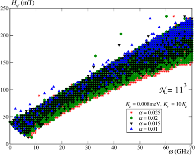
We stop this time evolution when two criteria are satisfied: First we require that , with a negative number. This condition is required to ensure switching. Accordingly, in Fig. 1, we show the - phase diagram for the NSA model with different values of (). We see that indeed the phase diagram strongly depends on the switching criterion. More explicitly, for a given , a higher requires a higher frequency since more energy has to be pumped into the system from the rf field. On the other hand, at a given frequency , the larger the smaller is the critical . This can be understood by the fact that a small value of requires the system to be maintained halfway from the more stable (deeper) minimum and this requires a stronger field. In all subsequent results of the present study, we adopted the most stringent criterion, i.e. with the largest value of . At finite temperature, this would insure the highest thermal stability for the magnetic state of the system. In fact, a second criterion is necessary in order to ensure that the final magnetic moment remains in the minimum reached after switching. For this, we require that the fluctuations of the net magnetic moment decay to a small value, i.e. .
Now we discuss the effect of the damping parameter in Eq. (5). The present study is concerned with the magnetization dynamics at very low temperatures. As such, the magnetization switching can only be achieved by going over the energy barrier. In this case, the role of the damping term in Eq. (5) is to drive the net magnetic moment of the nanomagnet towards the effective field and thus to push the system into its global energy minimum. In particular, it does not affect the time trajectory of the net magnetic moment during its switching process. However, the value of does have a bearing on the computing time needed for the system to reach equilibrium, i.e. its global minimum, but does not affect the global switching diagram as far as the values of and are concerned. This is indeed confirmed by the results shown in Fig. 2. Consequently, this study and all subsequent results have been obtained for a fixed value of , stated after Eq. (5).
In general, it is a rather involved task to deal with the dynamics within a many-spin approach, especially the calculation of relaxation rates, magnetization reversal, AC susceptibility and so on. Indeed, it is a formidable task to perform a detailed analysis of the various critical points (minima, maxima, saddle points) of the energy which are required for the study of the relaxation processes (J.S. Langer, Theory of Nucleation Rates, 1968; J.S. Langer, Statistical theory of the decay of metastable states, 1969; H. Kachkachi, Effect of exchange interaction on superparamagnetic relaxation, 2003; H. Kachkachi, Dynamics of a nanoparticle as a one-spin system and beyond, 2004). In the particular case of the present study of the switching - phase diagram, it is not so easy to analyze the various switching mechanisms. As such, it is desirable to replace the many-spin problem by some effective macroscopic model. Accordingly, it has been shown (Garanin and Kachkachi, 2003; H. Kachkachi and E. Bonet, Surface-induced cubic anisotropy in nanomagnets, 2006; H. Kachkachi, Effects of spin non-collinearities in magnetic nanoparticles, 2007; R. Yanes, O. Fesenko-Chubykalo, H. Kachkachi, D.A. Garanin, R. Evans, R. W. Chantrell, Effective anisotropies and energy barriers of magnetic nanoparticles within the Néel’s surface anisotropy, 2007) that, under some conditions which are quite plausible for today’s state-of-the-art grown nanomagnets, namely of weak surface disorder, one can map this atomistic approach onto a macroscopic model for the net magnetic moment defined in Eq. (6), evolving in the effective potential (H.O.T. = higher-order terms)
| (7) |
We remark in passing that there is a rich literature of works (G. Bertotti, I. Mayergoyz, and C. Serpico, Analysis of instabilities in nonlinear Landau-Lifshitz-Gilbert dynamics under circularly polarized fields, 2002; S. I. Denisov, T.V. Lyutyy, and P. Hänggi, Magnetization of nanoparticle systems in a rotating magnetic field, 2006; J. Podbielski, D. Heitmann, and D. Grundler, 2007; G. Woltersdorf and Ch. H. Back, 2007; Cai et al., 2013) that study, in the macrospin approach, the switching of a nanomagnet assisted by the circularly polarized microwave field in Eq. (3) and, in some cases, analytical analysis is performed in order to determine the various stable states of the system and their optimal switching paths. In the present situation, the effective model in Eq. (7), as compared to the macrospin studied in the cited works, takes into account the internal structure and boundary effects in the nanomagnet, and these lead to the quartic term in the energy potential in Eq. (7). Because of the latter, highly nonlinear contributions are brought in and it is thereby difficult, if not impossible, to carry out similar analytical investigations even at equilibrium.
In the sequel, we will refer to Eqs. (7, 6) as the effective-one-spin problem (EOSP) while the many-spin nanomagnet, described by the set of equations (1) and (4), will be referred to as the many-spin problem (MSP). We emphasize that the two leading terms in Eq. (7) have coefficients and whose value and sign are functions of the atomistic parameters ( etc) and of the size and shape of the nanomagnet (Garanin and Kachkachi, 2003; H. Kachkachi, Effects of spin non-collinearities in magnetic nanoparticles, 2007; Garanin, 2018; R. Yanes, O. Fesenko-Chubykalo, H. Kachkachi, D.A. Garanin, R. Evans, R. W. Chantrell, Effective anisotropies and energy barriers of magnetic nanoparticles within the Néel’s surface anisotropy, 2007). Moreover, we note that both the core and surface may contribute to and . For example, when the anisotropy in the core is uniaxial, , where is the number of atoms in the core, see Ref. H. Kachkachi and E. Bonet, Surface-induced cubic anisotropy in nanomagnets, 2006. In fact, even in this case the quartic term appears and is a pure surface contribution. Regarding the coefficient of the quartic contribution, for a sphere we have (or ) where is a surface integral (Garanin and Kachkachi, 2003) and for a cube, (Garanin, 2018). The details of the conditions under which this effective model is applicable are discussed in Ref. Garanin and Kachkachi, 2003 and may be summarized as follows: the spin misalignment (or canting) should not be too strong. Therefore, the effective model can be built for a nanomagnet whose surface anisotropy constant , as compared to the spin-spin exchange coupling , is small (). On the other hand, the nanomagnet size should not be too large for it to be considered as a single magnetic domain, for a given underlying material.
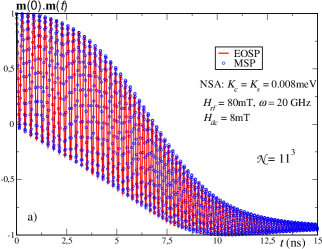
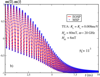
In Fig. 3 we plot the time evolution of the net magnetic moment of a nanomagnet of size with the parameters indicated in the legend, for both the NSA (a) and TUA (b) and . In both situations, we see that for the surface anisotropy constant considered, the effective model (EOSP) recovers very well the behavior of the many-spin nanomagnet (MSP). Hence, in the sequel all results will be presented for the EOSP model, since the corresponding calculation spares us much CPU time while producing the same results, as long as the validity conditions for EOSP are met, which will be the case for all subsequent calculations [See discussion below]. Note that when the size and the other parameters of the MSP system are varied, the coefficients and of the EOSP model (7) are accordingly adjusted.
II More results and discussion
II.1 Temporal evolution
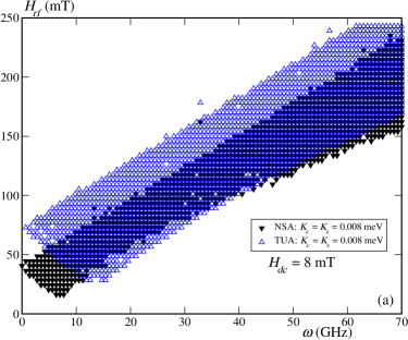
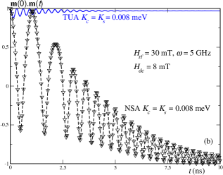
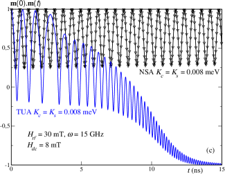
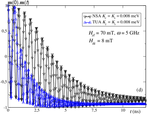
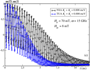
In Fig. 4 we plot the results for a nanomagnet of size . The upper panel is the () phase diagram for TUA and NSA. In both models, the value of the anisotropy constant is the same for all spins within the nanomagnet. The physical parameters used are given in the caption and legends. The result in Fig. 4(a) shows that the NSA model with a nonuniform distribution of the anisotropy easy axes allows for switching in a region with smaller amplitude and frequency (left lower corner of the diagram) than the TUA model. On the other hand, the latter allows for a wider domain of switching field intensities, though of higher values. Next, the graph in Fig. 4(b) shows that, for a given amplitude and frequency of , switching is obtained with NSA and not with TUA. Again, this means that the misalignment induced by the Néel surface anisotropy favors switching. This result, however, depends on frequency as is shown by the graphs in Fig. 4(b) and (c). Now, comparing the graphs in Figs. 4(b) and (d), we see that switching is achieved within TUA but at the expense of a higher rf field amplitude. Under this field, and higher frequencies, switching is achieved in both models, as witnessed by the graph in Fig. 4(e).
The general explanation of these observations resides in the anisotropy configuration within the two models, NSA and TUA, for a box-shaped nanomagnet. For the TUA model, the anisotropy is textured with all easy axes pointing in the (vertical) direction. So, on the horizontal facets, NSA and TUA have the same easy axis(H. Kachkachi and E. Bonet, Surface-induced cubic anisotropy in nanomagnets, 2006). However, on the other four facets and along the edges, NSA has a perpendicular effective anisotropy direction. As such, in the TUA model the effective anisotropy field is stronger (more rigid) and thereby the magnetization switching requires higher external fields and/or higher frequencies.
II.2 Effect of surface anisotropy ()
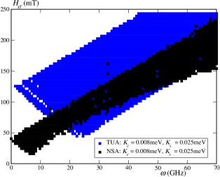
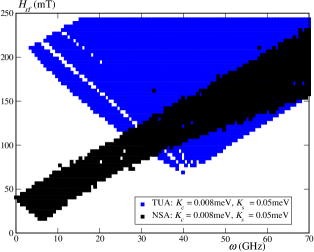
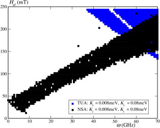
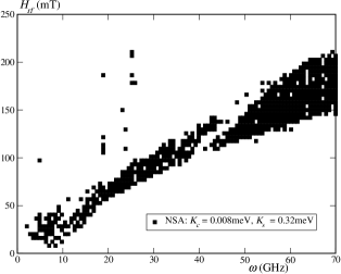
The first three phase diagrams in Fig. 5 are obtained for TUA and NSA models with the same (fixed) anisotropy constant in the core and increasing anisotropy constant at the surface. Comparing the three diagrams, we first observe that the TUA model renders a phase diagram that shifts to the right along the diagonal, i.e. towards higher amplitudes and frequencies of the rf field. This is due to the fact that as increases it makes the system with textured anisotropy (i.e. TUA) more rigid. On the other hand, the NSA seems to be less sensitive to the increase of , apart from a small shift to lower amplitudes of . In fact, once the latter has reached the sufficient value for inducing a nonuniform spin configuration, the switching mechanism remains the same. However, as is further increased, the phase diagram shows more “holes” which means that switching is no longer possible for all field amplitudes and frequencies. This is shown by the last phase diagram in Fig. 5. In fact, when surface anisotropy is strong enough (but not too strong) as to induce spin misalignment, several generations of spin waves are created with different amplitudes and frequencies (Yukalov, 2005; Yukalov et al., 2008; D. A. Garanin, H. Kachkachi and L. Reynaud, Magnetization reversal and nonexponential relaxation via instabilities of internal spin waves in nanomagnets, 2008; D. A. Garanin and H. Kachkachi, Magnetization reversal via internal spin waves in magnetic nanoparticles, 2009), but only those modes that are at resonance or whose frequencies match the rf field frequency do participate in the switching mechanism (J. Podbielski, D. Heitmann, and D. Grundler, 2007; G. Woltersdorf and Ch. H. Back, 2007). On the other hand, the results in the lower right panel of Fig. 5 show that the effective model (EOSP) reaches the limits of its validity regarding the parameters . Indeed, in Refs. (H. Kachkachi and E. Bonet, Surface-induced cubic anisotropy in nanomagnets, 2006; R. Yanes, O. Fesenko-Chubykalo, H. Kachkachi, D.A. Garanin, R. Evans, R. W. Chantrell, Effective anisotropies and energy barriers of magnetic nanoparticles within the Néel’s surface anisotropy, 2007), it was checked that the validity limit on is about for a simple cubic lattice and for a face-centered cubic lattice.
Summing up, it is clearly demonstrated that surface effects, as exemplified by the NSA model, open up switching channels for relatively low rf fields intensities and frequencies, as compared to the textured-anisotropy model TUA. This is seen in all phase diagrams in Fig. 5 and in subsequent ones. Indeed, they all exhibit a switching area that stretches to the left lower corner, though they remain narrower at higher intensities and frequencies.
In general, in a nanomagnet with nonuniform anisotropy, transverse spin waves are excited which are not necessarily spin waves in an equilibrium state. These transverse spin fluctuations trigger spin motion which may grow up into a coherent dynamics and ultimately induce magnetization switching(Yukalov, 2005; Yukalov et al., 2008; D. A. Garanin, H. Kachkachi and L. Reynaud, Magnetization reversal and nonexponential relaxation via instabilities of internal spin waves in nanomagnets, 2008; D. A. Garanin and H. Kachkachi, Magnetization reversal via internal spin waves in magnetic nanoparticles, 2009).
II.3 Size effect
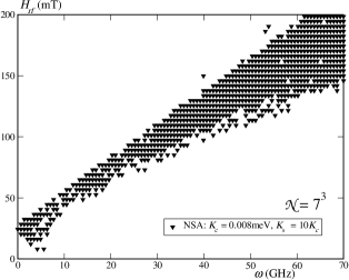
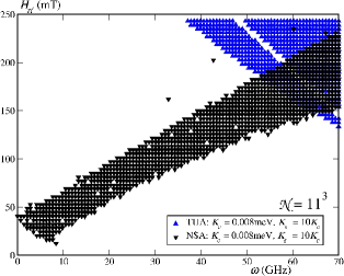
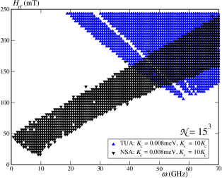
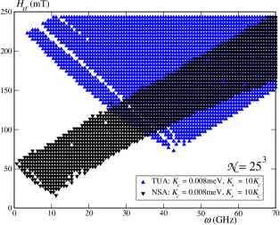


In Fig. 6 we plot the - phase diagram for both the NSA and TUA nanomagnets of varying size (cube side), which corresponds to a ratio of surface-to-total number of spins equal to , respectively. The anisotropy constants are chosen so that .
First, we see that, in what regards the TUA model, as the size increases ( decreases) the phase diagram extends towards lower amplitudes and frequencies of the rf field. For example, for the size , corresponding to , i.e. with a large surface contribution (in number of spins and anisotropy strength), the phase diagram of TUA “disappears” which means that switching in this case would require much higher values of the rf field amplitude and frequency. On the other hand, upon increasing the size, the surface contribution decreases in terms of spins number, and thereby the core effective anisotropy becomes relatively stronger than that on the surface and, as such, low-frequency and small-field dynamics takes over. This is illustrated in Fig. 6 by the results for size .
The situation for the NSA model is somewhat reversed. First, for all these sizes and the corresponding surface contributions, magnetization switching is achieved for all rf fields (amplitude and frequency) in the explored ranges. Moreover, the NSA phase diagram widens in the lower left corner of the diagram, i.e. for lower amplitudes and frequencies of the rf field when decreases. This means that, as was shown by the results in Fig. 5, when the contribution of surface anisotropy dominates, there are only some specific modes that contribute to switching.
As can be seen in Fig. 6, at very large system sizes (e.g. ), the surface contribution becomes negligible and the two models tend to (asymptotically) yield the same switching diagram, since the black diagram widens and the blue one shrinks. This is mainly due to the fact that as , the effective anisotropy in the two models becomes the same.
III Conclusion
We have studied the effect of surface anisotropy, and the spin misalignment it induces, on the magnetization switching in a many-spin nanomagnet subjected to an rf magnetic field, on top of a DC magnetic field. Our study is based on the numerical solution of the damped Landau-Lifshitz equation for exchange-coupled atomic spins.
We have demonstrated that surface effects, as exemplified by Néel’s model for surface atoms, open up switching channels with relatively low rf fields intensities and frequencies, as compared to the model with parallel easy axes, or the so-called macrospin model. In general, these favorable switching conditions depend on the size and shape of the nanomagnet and, of course, on the underlying magnetic properties and energy parameters. However, thanks to today’s state of the art facilities for growing well defined nanomagnets, it is possible to meet most of these conditions and achieve an optimized magnetization switching in these nanoscale systems. On the other hand, most of the systems available today are ensembles of interacting nanomagnets with controlled separation and spatial organization. The present study has been devoted to a single nanomagnet in order to investigate the (intrinsic) surface effects on the magnetization switching mechanisms. It will be of fundamental and practical interest to extend this study to interacting nanomagnets and to compare with measurements on assemblies of different concentrations.
References
- C. Thirion, W. Wernsdorfer and D. Mailly, Switching of magnetization by nonlinear resonance studied in single nanoparticles (2003) C. Thirion, W. Wernsdorfer and D. Mailly, Switching of magnetization by nonlinear resonance studied in single nanoparticles, Nature 2, 524 (2003).
- Woltersdorf et al. (2007) G. Woltersdorf, O. Mosendz, B. Heinrich, and C. H. Back, Phys. Rev. Lett. 99, 246603 (2007).
- N. Barros, M. Rassam, H. Jirari and H. Kachkachi, Optimal switching of a nanomagnet assisted by microwaves (2011) N. Barros, M. Rassam, H. Jirari and H. Kachkachi, Optimal switching of a nanomagnet assisted by microwaves, Phys. Rev. B 83, 144418 (2011).
- N. Barros, M. Rassam and H. Kachkachi, Microwave-assisted switching of a nanomagnet: Analytical determination of the optimal microwave field (2013) N. Barros, M. Rassam and H. Kachkachi, Microwave-assisted switching of a nanomagnet: Analytical determination of the optimal microwave field, Phys. Rev. B 88, 014421 (2013).
- Suto et al. (2017) H. Suto, T. Kanao, T. Nagasawa, K. Kudo, K. Mizushima, and R. Sato, Appl. Phys. Lett. 110, 262403 (2017).
- Sun and Wang (2006) Z. Z. Sun and X. R. Wang, Phys. Rev. B 74, 132401 (2006).
- Cai et al. (2013) L. Cai, D. A. Garanin, and E. M. Chunovsky, Phys. Rev. B 87, 024418 (2013).
- Taniguchi et al. (2016) T. Taniguchi, D. Saida, Y. Nakatani, and H. Kubota, Phys. Rev. B 93, 014430 (2016).
- D. A. Garanin, H. Kachkachi and L. Reynaud, Magnetization reversal and nonexponential relaxation via instabilities of internal spin waves in nanomagnets (2008) D. A. Garanin, H. Kachkachi and L. Reynaud, Magnetization reversal and nonexponential relaxation via instabilities of internal spin waves in nanomagnets, Europhys. Lett. 82, 17007 (2008).
- D. A. Garanin and H. Kachkachi, Magnetization reversal via internal spin waves in magnetic nanoparticles (2009) D. A. Garanin and H. Kachkachi, Magnetization reversal via internal spin waves in magnetic nanoparticles, Phys. Rev. B 80, 014420 (2009).
- Seki et al. (2023) T. Seki, K. Utsimiya, K. Nozaki, H. Imamura, and K. Takanashi, Nature Communications 4, 1726 (2023).
- Yamaji and Imamura (2016) T. Yamaji and H. Imamura, Appl. Phys. Lett. 109, 192406 (2016).
- H. Kachkachi and D.A. Garanin (2005) H. Kachkachi and D.A. Garanin, in Surface effects in magnetic nanoparticles, edited by D. Fiorani (Springer, Berlin, 2005) p. 75.
- Schmool and Kachkachi (2015) D. S. Schmool and H. Kachkachi (Academic Press, 2015) pp. 301–423.
- Schmool and Kachkachi (2016) D. Schmool and H. Kachkachi (Academic Press, 2016) pp. 1–101.
- Kanso et al. (2019) H. Kanso, R. Patte, V. Baltz, and D. Ledue, Phys. Rev. B 99, 054410 (2019).
- Iglesias and Kachkachi (2021) Ò. Iglesias and H. Kachkachi, Single nanomagnet behaviour: Surface and finite-size effects, in New Trends in Nanoparticle Magnetism, edited by D. Peddis, S. Laureti, and D. Fiorani (Springer International Publishing, Cham, 2021) pp. 3–38.
- D.A. Dimitrov and Wysin, Effects of surface anisotropy on hysteresis in fine magnetic particles (1994) D.A. Dimitrov and Wysin, Effects of surface anisotropy on hysteresis in fine magnetic particles, Phys. Rev. B 50, 3077 (1994).
- O. Iglesias and A. Labarta, Finite-size and surface effects in maghemite nanoparticles: Monte Carlo simulations (2001) O. Iglesias and A. Labarta, Finite-size and surface effects in maghemite nanoparticles: Monte Carlo simulations, Phys. Rev. B 63, 184416 (2001).
- H. Kachkachi and M. Dimian, Hysteretic properties of a magnetic particle with strong surface anisotropy (2002) H. Kachkachi and M. Dimian, Hysteretic properties of a magnetic particle with strong surface anisotropy, Phys. Rev. B 66, 174419 (2002).
- N. Kazantseva, D. Hinzke, U. Nowak, R. W. Chantrell, U. Atxitia, and O. Chubykalo-Fesenko, Towards multiscale modeling of magnetic materials: Simulations of FePt (2008) N. Kazantseva, D. Hinzke, U. Nowak, R. W. Chantrell, U. Atxitia, and O. Chubykalo-Fesenko, Towards multiscale modeling of magnetic materials: Simulations of FePt, Phys. Rev. B 77, 184428 (2008).
- Fraile Rodríguez et al. (2010) A. Fraile Rodríguez, A. Kleibert, J. Bansmann, A. Voitkans, L. J. Heyderman, and F. Nolting, Phys. Rev. Lett. 104, 127201 (2010).
- R. Bastardis, U. Atxitia, O. Chubykalo-Fesenko, and H. Kachkachi, Unified decoupling scheme for exchange and anisotropy contributions and temperature-dependent spectral properties of anisotropic spin systems (2012) R. Bastardis, U. Atxitia, O. Chubykalo-Fesenko, and H. Kachkachi, Unified decoupling scheme for exchange and anisotropy contributions and temperature-dependent spectral properties of anisotropic spin systems, Phys. Rev. B 86, 094415 (2012).
- S. I. Denisov, T.V. Lyutyy, and P. Hänggi, Magnetization of nanoparticle systems in a rotating magnetic field (2006) S. I. Denisov, T.V. Lyutyy, and P. Hänggi, Magnetization of nanoparticle systems in a rotating magnetic field, Phys. Rev. Lett. 97, 227202 (2006).
- L. Néel, Anisotropie magnétique superficielle et surstructures d’orientation (1954) L. Néel, Anisotropie magnétique superficielle et surstructures d’orientation, J. Phys. Radium 15, 225 (1954).
- R. Skomski and J.M.D. Coey (1999) R. Skomski and J.M.D. Coey, Permanent Magnetism, Studies in Condensed Matter Physics Vol. 1 (IOP Publishing, London, 1999).
- K.B. Urquhart, B. Heinrich, J.F. Cochran, A.S. Arrott, and K. Myrtle, Ferromagnetic resonance in ultrahigh vacuum of bcc Fe films grown on Ag(001)(1988) (001) K.B. Urquhart, B. Heinrich, J.F. Cochran, A.S. Arrott, and K. Myrtle, Ferromagnetic resonance in ultrahigh vacuum of bcc Fe(001) films grown on Ag(001), J. Appl. Phys. 64, 5334 (1988).
- R. Perzynski and Yu.L. Raikher (2005) R. Perzynski and Yu.L. Raikher, in Surface effects in magnetic nanoparticles, edited by D. Fiorani (Springer, Berlin, 2005) p. 141.
- J.S. Langer, Theory of Nucleation Rates (1968) J.S. Langer, Theory of Nucleation Rates, Phys. Rev. Lett. 21, 973 (1968).
- J.S. Langer, Statistical theory of the decay of metastable states (1969) J.S. Langer, Statistical theory of the decay of metastable states, Ann. Phys. (N.Y.) 54, 258 (1969).
- H. Kachkachi, Effect of exchange interaction on superparamagnetic relaxation (2003) H. Kachkachi, Effect of exchange interaction on superparamagnetic relaxation, Eur. Phys. Lett. 62, 650 (2003).
- H. Kachkachi, Dynamics of a nanoparticle as a one-spin system and beyond (2004) H. Kachkachi, Dynamics of a nanoparticle as a one-spin system and beyond, J. Mol. Liquids 114, 113 (2004).
- Garanin and Kachkachi (2003) D. A. Garanin and H. Kachkachi, Phys. Rev. Lett. 90, 065504 (2003).
- H. Kachkachi and E. Bonet, Surface-induced cubic anisotropy in nanomagnets (2006) H. Kachkachi and E. Bonet, Surface-induced cubic anisotropy in nanomagnets, Phys. Rev. B 73, 224402 (2006).
- H. Kachkachi, Effects of spin non-collinearities in magnetic nanoparticles (2007) H. Kachkachi, Effects of spin non-collinearities in magnetic nanoparticles, J. Magn. Magn. Mater. 316, 248 (2007).
- R. Yanes, O. Fesenko-Chubykalo, H. Kachkachi, D.A. Garanin, R. Evans, R. W. Chantrell, Effective anisotropies and energy barriers of magnetic nanoparticles within the Néel’s surface anisotropy (2007) R. Yanes, O. Fesenko-Chubykalo, H. Kachkachi, D.A. Garanin, R. Evans, R. W. Chantrell, Effective anisotropies and energy barriers of magnetic nanoparticles within the Néel’s surface anisotropy, Phys. Rev. B 76, 064416 (2007).
- G. Bertotti, I. Mayergoyz, and C. Serpico, Analysis of instabilities in nonlinear Landau-Lifshitz-Gilbert dynamics under circularly polarized fields (2002) G. Bertotti, I. Mayergoyz, and C. Serpico, Analysis of instabilities in nonlinear Landau-Lifshitz-Gilbert dynamics under circularly polarized fields, J. Appl. Phys. 91, 7556 (2002).
- J. Podbielski, D. Heitmann, and D. Grundler (2007) J. Podbielski, D. Heitmann, and D. Grundler, Phys. Rev. Lett. 99, 207202 (2007).
- G. Woltersdorf and Ch. H. Back (2007) G. Woltersdorf and Ch. H. Back, Phys. Rev. Lett. 99, 227207 (2007).
- Garanin (2018) D. A. Garanin, Phys. Rev. B 98, 054427 (2018).
- Yukalov (2005) V. I. Yukalov, Phys. Rev. B 71, 184432 (2005).
- Yukalov et al. (2008) V. I. Yukalov, V. K. Henner, and P. V. Kharebov, Phys. Rev. B 77, 134427 (2008).