Quantifying Network Similarity using Graph Cumulants
Abstract
How might one test the hypothesis that networks were sampled from the same distribution? Here, we compare two statistical tests that use subgraph counts to address this question. The first uses the empirical subgraph densities themselves as estimates of those of the underlying distribution. The second test uses a new approach that converts these subgraph densities into estimates of the graph cumulants of the distribution (without any increase in computational complexity). We demonstrate — via theory, simulation, and application to real data — the superior statistical power of using graph cumulants. In summary, when analyzing data using subgraph/motif densities, we suggest using the corresponding graph cumulants instead.
Keywords: subgraph counts, two-sample test, graph cumulants, graph moments, network comparison, motif analysis, graphons
1 Statement of the Problem
In this paper, we use statistics based on subgraph counts to address the following problem:
Given two samples, and , each containing graphs sampled i.i.d. from unknown distributions and , respectively, the goal is to infer whether and are different distributions.
2 What we are Doing (Motivation)
The theory for statistical analysis of i.i.d. data (e.g., the height and weight of different breeds of dogs) is well-established (Casella and Berger, 2021; Stuart and Kendall, 1963). However, when the data of interest are interactions (e.g., who plays with whom in the dog park), a similar consensus has not yet been reached (Orbanz, 2017).
To analyze such networks of interactions, one common approach is to use statistics based on counts of small substructures (i.e., subgraphs or “motifs”) (Aliakbarpour et al., 2018; Maugis et al., 2020; Pattillo et al., 2013; Xia et al., 2019). For example: the densities of “k-star” subgraphs provide increasingly detailed information about a network’s degree distribution (Rauh, 2017), and the density of cliques of various sizes gives information about the scale of its clustering (Ouyang et al., 2019).
To make meaningful comparisons, one must first answer the question: “Compared to what?” The frequently-used clustering coefficient opts to divide the number of “complete” triangles by the number of “incomplete” triangles (Newman, 2001). The often-cited configuration model compares the observed subgraph counts with those of random networks with the same degree distribution (Alon, 2007; Barabási and Albert, 1999).
The recently-proposed graph cumulants (Gunderson and Bravo-Hermsdorff, 2020) offer a natural set of statistics based on a combinatorial view of cumulants (e.g., mean, variance, skew, kurtosis, etc.). Graph cumulants compare the density of a substructure in a network to the density that would be expected due to the prevalence of smaller substructures, thereby quantifying an intuitive notion of “excess propensity” for that substructure.
It is well-known that subgraph densities are useful for characterizing individual networks (Bickel et al., 2011; Bhattacharyya and Bickel, 2015) and for comparing different networks (Maugis et al., 2020; Bhattacharya et al., 2022; Zhang and Xia, 2022; Jin et al., 2021). A few works have also used statistics that combine subgraph densities to compare networks. In particular, Gao and Lafferty (2017) uses two statistics (one involving edge and -star densities, and the other involving edge and triangle densities) to devise a test for distinguishing an Erdős-Rényi model from an alternative stochastic block model (SBM).
Here, we describe a simple statistical test for comparing networks based on graph cumulants. For comparison, we consider the analogous test based on graph moments (i.e., subgraph densities) (Maugis et al., 2020). Our results strongly suggest that graph cumulants should be the default choice of statistics for problems involving subgraph counts.
3 What we are Not Doing (Related Work)
There are many ways to compare networks (Tantardini et al., 2019). Here, we describe some other common approaches, highlighting their differences with the setting considered in this paper.
3.1 Spectral Methods
Broadly, these methods use the eigendecomposition of matrices associated with the network, such as the adjacency matrix or the graph Laplacian (Chen et al., 2020; Bravo-Hermsdorff and Gunderson, 2019; Mukherjee et al., 2016). Here, we focus instead on statistics based on the frequency of small subgraphs. These two approaches are complementary (Lovász, 2012); flavorfully, spectral methods are more sensitive to the graph’s global structure (its “shape”), whereas methods based on subgraph frequencies are more sensitive to the graph’s local structure (its “texture”).
3.2 Matching Nodes
When the networks being compared have the same set of unique names for all their nodes (Ghoshdastidar et al., 2020; Tang et al., 2017), it is highly advantageous for statistical tests to incorporate this one-to-one mapping (e.g., when comparing fMRI data of different subjects, it helps to assume that their hippocampi are sufficiently analogous). However, such information is not always available (e.g., when comparing the social interactions within different schools). This work addresses the latter problem; the nodes are considered to be indistinguishable (i.e., exchangeable), and only the statistics of their pairwise interactions (i.e., their edges) are known to the tests.
3.3 Obtaining Significance by Sampling
Many tests for comparing networks require sampling from the inferred distributions to estimate the significance of their differences. Common examples include the use of configuration models (Masuda et al., 2018), exponential random graph models (An, 2016), and geometric random graph models (Asta and Shalizi, 2014). Such methods are typically computationally intensive, rendering them difficult (or impossible) to implement in practice (Ginoza and Mugler, 2010). The two tests considered in this paper sidestep this issue entirely, analytically computing the significance of the observed differences between the networks.
4 How we Name Things (Notation)
A capital denotes a single graph with nodes. All graphs are assumed to be undirected, unweighted, simple graphs.111This is for simplicity of presentation; the tests we describe here naturally extend to networks with additional information, such as directed edges, weighted edges, and node attributes (Gunderson and Bravo-Hermsdorff, 2020). A calligraphic denotes a distribution over such graphs. All graph distributions are assumed to be generated by a single graphon (Lovász, 2012) (see Section 7).222Again, this assumption may be relaxed. A bold denotes a sample of graphs from such a distribution. All graphs in a sample are assumed to have the same number of nodes.
A plebeian denotes a subgraph. An emboldened denotes a set of subgraphs. The set of subgraphs with at most edges is denoted by , and the restriction to connected subgraphs is denoted by (e.g., and ). Parenthetical superscripts are also used to distinguish the covariance matrices of graph moments from those of graph cumulants .
The statistics we consider here, namely, graph moments and graph cumulants, have associated with them a particular subgraph (see Section 5). denotes the graph moment (associated with subgraph ) of a distribution (see Section 5.1), and the corresponding graph cumulant (see Section 5.2). A bold (or ) denotes a vector of graph moments (or cumulants), one for each subgraph in .
5 Two Statistics based on Subgraphs (What we Measure)
We first define graph moments (Section 5.1), the statistics to which we compare our new method. Then we describe how to convert these to graph cumulants (Section 5.2), the statistics used by our new method.
5.1 Graph Moments (The Typically-used Statistics)
When discussing counts of a subgraph in some larger graph , it is important to distinguish between induced counts and homomorphism counts (Chen et al., 2008); here we are using the latter. Another important distinction is that we are using injective homomorphism counts. To obtain these counts, first consider all mappings from the nodes of to the nodes of .
Injective refers to a condition on these node mappings: consider only those mappings that do not send different nodes in to the same node in .
Homomorphism refers to how we decide which of those (injective) mappings are “counts”: those for which has edges at all the locations where there are edges in (i.e., it is still a count even if there are additional edges in ).
Out of all injective mappings from the nodes of to the nodes of , the fraction that are “counts” is known as the injective homomorphism density (Lovász, 2012). These densities are the graph moments of a graph , denoted by .
5.2 Graph Cumulants (The New Statistics)
Graph cumulants were recently introduced by Gunderson and Bravo-Hermsdorff (2020). We first review the defining features of cumulants, highlighting a less-well-known combinatorial definition (Section 5.2.1). We then describe the analogue for graphs (Section 5.2.2).
5.2.1 Combinatorial Cumulants (Background)
First, consider a scalar-valued random variable sampled from some distribution . The -order moment of is the expectation of the power of : . These moments may be combined into certain polynomial expressions, known as the cumulants (e.g., mean, variance, skew, kurtosis, etc.).
Cumulants have a uniquely defining property related to sums of independent random variables (Rota and Shen, 2000): the cumulants of the resulting sum are equal to the sum of the cumulants of those independent random variables (e.g., , when and are independent). This is essentially the reason behind the central limit theorem and the ubiquity of the Gaussian distribution (Gnedenko and Kolmogorov, 1954; Hald, 2000).
While the classical cumulants are often defined via the cumulant generating function, they also have an equivalent combinatorial definition in terms of a Möbius transform (see Section 12) (Kardar, 2007; McCullagh, 1987; Lehner, 2004). Namely, the moment can be expressed as a sum of cumulants of order and lower, corresponding to all partitions of unique elements (see Figure 1, top three rows). In particular, for our scalar-valued example:
| (1) |
where is the moment, is the cumulant, is the set of all partitions of unique elements (i.e., a set of non-overlapping subsets, or “blocks”, whose union contains all elements), is one such partition, is a block in partition , and is the number of elements in block .
Equation 1 may be rearranged to obtain expressions for the cumulants in terms of moments. For example, the third (classical) cumulant (the “skew”) is: . This combinatorial definition makes the generalization to random variables with additional structure, such as graphs, more transparent.
5.2.2 Graph Cumulants (Definition)
Before describing graph cumulants, it is worth mentioning a subtle point. Notice that Equation 1 relates the moments and cumulants of the distribution (and not of any finite sample ). While this distinction is somewhat pedantic for graph moments (see Section 7.1.1), the combinatorial definition of cumulants (classical or graphical) should only be applied to distributions.
The moments and cumulants of real-valued random variables are indexed by their order . For graph-valued random variables, moments (Lovász and Szegedy, 2010; Bickel et al., 2011) and cumulants (Gunderson and Bravo-Hermsdorff, 2020) are now indexed by subgraphs , with order given by the number of edges in .
To apply the combinatorial definition (Equation 1) to networks, the partitioning of the edges of the subgraphs must respect their connectivity (see Figure 1, bottom row), i.e.:
| (2) |
where is the set of edges forming subgraph , is the set of all partitions of these edges, and is the subgraph formed by the edges in .
Again, these may be rearranged to obtain the graph cumulants in terms of the graph moments . For example, the (-order) graph cumulant associated with the path graph with edges is:
| (3) |
6 The Statistical Tests (How we Compare Graphs)
In this section, we describe the ways in which we ensured that the tests use the statistics and in the same way, so as to compare graph cumulants on an equal footing with the corresponding subgraph densities/moments. In particular, both tests have the same structure (Section 6.1), rely on the same assumptions (Section 6.2), and have the same computational complexity (Section 6.3).
6.1 Same Structure
To compare graph moments and graph cumulants on the same footing, we use them as analogous inputs to the same simple statistical test:
-
1.
choose , the maximum order of the subgraph statistics being considered;
-
2.
for each sample, estimate its distribution using these subgraph statistics;
-
3.
quantify the difference between distributions
using a notion of distance for the space of these subgraph statistics.
In particular, we consider the graph moments/cumulants associated with , the set of connected subgraphs with at most edges. To measure the difference between two samples of graphs and , we use the squared Mahalanobis distance (Mahalanobis, 1936) between their inferred moments/cumulants:
| (4) | ||||
| (5) |
where is the vector of estimated moments of sample , and is the covariance estimate of the vector of estimated cumulants of sample , etc.
In Section 7, we describe how to compute these estimators.
6.2 Same Assumptions
We assume that the observed graphs in a sample were all obtained by subsampling nodes i.i.d. from a single (much larger) “graph” . In other words, we assume that each graph distribution is generated by an underlying graphon (Borgs et al., 2008; Lovász, 2012). This assumption allows for several notable simplifications (in particular, Equation 8) without changing the primary message.
In addition, the graph distributions induced by a graphon are dense, and have empirical subgraph densities that converge to a Gaussian distribution as (Bickel et al., 2011). As the empirical estimators of graph cumulants are linear combinations of the empirical subgraph densities (see Section 10), they also limit to a Gaussian distribution. Moreover, as the number of graphs per sample becomes large (), the averages will also approach a Gaussian distribution by the central limit theorem (see also Appendix A).
In light of these Gaussian limits, the well-established Mahalanobis distance (Anderson, 1958; Reiser, 2001) is appropriate for both tests considered in this paper. In Sections 8, 9, and 10, we show that (in contrast to moments) graph cumulants work well in practice, even when using this simple classical distance.
6.3 Same Complexity
The computational complexity of both tests is determined by the complexity of counting the relevant subgraphs. Computing the covariance matrices in Equations 4 and 5 requires counting connected subgraphs with at most edges (see Section 7.2).
For this paper, we use . To count all but the complete graph on nodes (), we follow an approach similar to that in Maugis et al. (2016). Beginning with the observed adjacency matrix, we require matrix multiplication and entry-wise operations (thereby taking time, where is the matrix multiplication exponent). For , we require multiplying an and an matrix, where is the number of edges.
Our approach is not the best one can do. Efficiently counting subgraphs is a highly active area of research (Ribeiro et al., 2021), with a variety of powerful algorithms (Ye et al., 2022; Pinar et al., 2017), especially for certain (realistic) classes of graphs (Bera et al., 2019; Chiba and Nishizeki, 1985; Bressan, 2021), and for particular subgraphs (e.g., triangles (Gui et al., 2019)). Asymptotics aside, substantial acceleration can be obtained through parallel computation (Dodeja et al., 2022; Biswas et al., 2020), and more recently through the use of machine learning techniques (Zhao et al., 2021; Liu et al., 2020).
7 How to Estimate the Statistics (What we Compute)
In Section 7.1, we describe unbiased estimators for the graph moments and cumulants, highlighting an important relationship between subgraph densities in the process (Equation 8). In Section 7.2, we build on this idea to describe the typical fluctuations of such sample statistics in terms of their covariance matrices.
7.1 Obtaining Unbiased Estimators (Getting the Mean)
7.1.1 For Graph Moments (Simple Substitution)
For a graphon model, graph moments are preserved under node subsampling:
| (6) |
Thus, the empirical graph moments are themselves unbiased estimators of the moments of the distribution from which they were sampled. In particular, for a sample of graphs:
| (7) |
7.1.2 For Graph Cumulants (Slightly Subtle)
To obtain the analogous estimators for graph cumulants, we must be slightly more careful, as products of graph moments are not preserved in expectation under node subsampling. Fortunately, for graphs sampled from a graphon, products of graph moments are equal to the moment of their disjoint union333Intuitively, nodes in disjoint components have nothing to do with each other, so the presence of edges in any component are independent from the presence of edges in the other. (Lovász, 2012; Maugis et al., 2020):
| (8) |
For example, using this relation in the expression for the cumulant associated with the path graph with edges (Equation 3) results in its unbiased estimator:
| (9) |
For a sample of graphs, the estimated cumulants of the underlying distribution are the average of the unbiased estimators of each individual graph:
| (10) |
7.2 Analytically Computing Significance (Getting the Covariance)
Consider sampling graphs from a distribution with known graph moments. The covariance between their observed graph moments is
| (11) |
The last term is trivial; as graph moments are preserved under node subsampling (Equation 6), the expectations of the empirical moments are exactly the moments of the underlying distribution. The first term, however, is the expectation of a product of graph moments.
Equation 8 applies to a single graphon . The analogous expression for the moments of a single finite graph requires considering all the ways that the nodes of the subgraphs could overlap (Maugis et al., 2020). Thus, estimating the covariance of the empirical graph moments/cumulants up to order requires the estimation of the distribution’s graph moments/cumulants up to order (as stated in Section 6.3). For example, in terms of injective homomorphism counts, we have the following expression:
| (12) |
The term corresponds to the four ways that the two nodes of the edge can be placed to overlap with the wedge (), the term corresponds to the two ways those nodes can be placed to turn a wedge into a triangle, and so on. Converting from counts to moments and taking the expectation allows one to express Equation 11 in terms of moments of the distribution.
As the graphs in each sample are i.i.d. and have the same number of nodes, the covariance of the sample graph moments is
| (13) |
As the unbiased graph cumulants are linear combinations of the sample graph moments, obtaining their covariance follows mutatis mutandis:
| (14) |
8 A Controlled Competition (Between the Tests)
We first describe the models we use to generate the synthetic data. We then describe how we summarize the quality of the statistical tests, with illustrations for some representative simulations. Asymptotic results as are presented in Appendix A.
8.1 Synthetic Data (A Pair of two-by-two SBMs)
We consider two graph distributions: one with heterogeneous degree distribution (but no community structure), and the other with community structure (but homogeneous degree distribution). Both distributions are Stochastic Block Models (SBMs) (Holland et al., 1983) with two equal-sized communities and expected edge density .
The heterogeneous SBM is parameterized by , with connectivity matrix:
| (15) |
where gives uniform connection probability between all pairs of nodes, and gives zero connection probability within one of the two communities.
The assortative SBM is parameterized by , with connectivity matrix:
| (16) |
where again gives uniform connection probability between all pairs of nodes, and gives zero connection probability between the two communities.
After fixing two such SBMs, each instantiation of a two-sample test involves “flipping two coins” to decide which distributions each of the two samples will come from. That is, the instantiations are split evenly between “different distributions” and “same distribution”, with the latter split evenly between the two SBMs.
8.2 ROC and AUC Curves (How we Compare Tests)
After computing the squared Mahalanobis distance between a pair of samples (Equations 4 and 5), we use a threshold to classify them as coming from the “same distribution” or “different distributions.” Each choice of threshold induces: a rate of false positives (incorrectly concluding that the distributions are different), and a rate of true positives (correctly concluding that the distributions are different). All possible threshold choices are summarized in a Receiver Operating Characteristic (ROC) curve (see Figure 2).
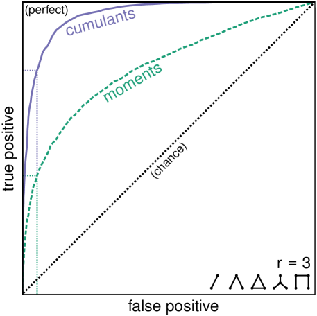
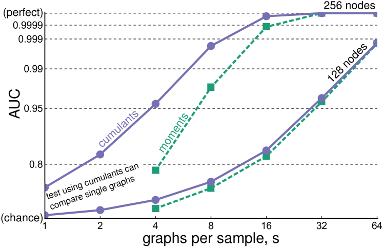
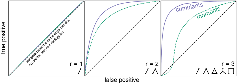
To compare ROC curves, we summarize them with a single scalar value, viz., the Area Under the Curve (AUC). Figure 3 compares the AUC for graphs with and nodes over a range of sample sizes. The use of graph cumulants consistently results in greater statistical power, especially when the number of graphs per sample is small (including the case of a single graph per sample, for which the test using moments is not applicable).
One might wonder if these results are sensitive to the model parameters and . While the values used to create the figures were judiciously chosen (e.g., such that the AUC spans the range from chance to perfect), the qualitative conclusions remain robust for (essentially) any parameter choice. In the next section, we show that the use of graph cumulants is similarly promising for applications to more realistic networks.
9 Studying the Tests in the Wild (Application to Real Networks)
Most real-world networks look rather different than the simulated graphs in the previous section. In this section, we compare the two tests using graphs sampled from more realistic graph distributions. In particular, we use gene interaction networks from four different species: Mouse, Rat, Human, and Arabidopsis (a small flowering plant related to cabbage and mustard), all curated by the FunCoup repository (Persson et al., 2021).
Although these networks have relatively similar edge densities, the differences are already enough for either test to easily distinguish samples from them using only the edge subgraph. As the differences between moments and cumulants only become apparent for subgraphs with more than one edge, we adjusted the networks being compared so they have the same edge density. This was done by removing the lowest-weight edges from the network with larger edge density until it had the same density as the other.444If one wishes to test if two distributions with different sparsities are otherwise the same, one could scale all subgraph densities by the edge density to the power of the number of edges in the subgraph. The effect of this adjustment can be seen in Figure 4 (left); both tests using edge can no longer distinguish between the samples.
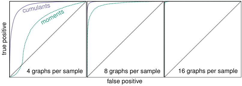
Each sample contains graphs, all obtained from one of these adjusted networks by subsampling its nodes. Specifically, each graph in a sample contains nodes in expectation (selected from the nodes in the adjusted network independently with probability ), and nodes in are connected by an edge if (and only if) their corresponding nodes in the adjusted network are connected by an edge. That is, is an induced subgraph of the adjusted network.
Figures 4 and 5 show that using graph cumulants to discriminate between these biological networks outperforms the analogous test using graph moments.
10 Why Cumulants do Better
Why does using graph cumulants consistently provide better statistical power? After all, unbiased graph cumulants are simply linear combinations of graph moments! (Section 7.1.2) Loosely, the reason is that graph distributions “look more Gaussian” when represented in terms of cumulants (as compared to moments).
Both tests measure differences between distributions using the squared Mahalanobis distance (Equations 4 and 5). As this measure depends only on the mean and covariance, there is a tacit assumption that the sample statistics are well-characterized by a multivariate Gaussian (Rao, 1992).
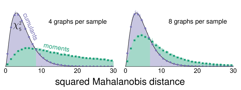
Indeed, if the subgraph statistics were precisely Gaussian, and their covariance known exactly, then the squared Mahalanobis distance between pairs of samples from the same distribution would in fact follow a distribution. However, as the sample statistics are not precisely Gaussian, and their covariance must be estimated, one should indeed expect some deviation from this limiting distribution.
As illustrated in Figure 6, when the graphs are sampled from the same distribution, the test using moments results in a distribution of squared Mahalanobis distances with overly-heavy tails. Whereas the distribution for the test using cumulants is well-characterized by the appropriate distribution, thereby allowing one to control the false positive rate.
11 The Main Message (Discussion)
Perhaps the most salient advantage of using graph cumulants (instead of the subgraph densities themselves) is the ability to compare distributions even when observing only a single graph from each (e.g., Figure 3).
At first glance, it may seem strange that one could make inferences about a distribution from a sample containing only a single “observation.” Indeed, this certainly does not work for scalar-valued random variables — a single observation provides no information about the spread of its underlying distribution.
Essentially, this difference arises because, in graphs, the data reside in the edges, but sampling is applied node-wise. Notationally, this manifests itself in our need to specify both (the number of nodes per graph) and (the number of graphs per sample), whereas the “quantity” of i.i.d. scalar data is specified by only the sample size.
Thus, there are two relevant limits: we may ask about the distributions of these statistics as either or become sufficiently large. As (with fixed ), both methods are asymptotically normal by the central limit theorem. In Appendix A, we show that using graph cumulants remains statistically advantageous even in this “classical” limit. As (with fixed ), graph cumulants appear to more properly exploit the multiplicity of the data within each graph, allowing for inference even when (see Appendix B).
In a sense, graph cumulants provide a more “natural” set of coordinates than the subgraph densities themselves. For example, the edge density is strongly correlated with the wedge moment . In contrast, “takes into account” the lower-order effect of edge density, rendering it “more orthogonal” to . In fact, for an Erdős-Rényi distribution, the covariance between the edge density and all other graph cumulants is precisely zero (see proof in Appendix C).
In practice, the covariance estimates for cumulants are more robust, leading to impressively accurate agreement with the classical distribution. This allows one to convert these statistics into precise probabilistic statements (e.g.: “What is the likelihood that two graphs were generated by different graphons?”). This notion of “graphonic similarity” between any pair of graphs is a remarkably general tool.
12 Promising Sequels (Future Directions)
Towards the goal of estimating the relevance of various subgraphs/motifs in an observed network, recent works (Bhattacharya et al., 2022; Zhang and Xia, 2022) have provided higher-order characterizations of the sampling distributions of (appropriately rescaled) estimators of subgraph densities for various regimes and model assumptions. Given the success of graph cumulants compared to the bare densities/moments in determining network similarity, a natural step to help in this endeavor is to provide such characterizations for the estimators of graph cumulants (e.g., by generalizing the result in Appendix C to arbitrary graphons and pairs of subgraphs).
It might be argued that intelligent feature engineering has been rendered moot by powerful supercomputers fitting deep neural networks to big data. Nonetheless, some of the most notable breakthroughs in machine learning have been the result of architectures with cleverly engineered priors (e.g., convolutional neural networks for computer vision tasks (LeCun et al., 1998; Khan et al., 2018), and transformers for natural language processing tasks (Vaswani et al., 2017; Chan et al., 2022)). Like the edge and orientation detection cells in the first layers of visual processing (Hubel and Wiesel, 1959; Gabbiani and Cox, 2017), graph cumulants offer a principled first layer of contrastive features when looking at the relationships between edges in networks.
As a coda, we highlight a compelling analogy between the conversion between induced subgraph densities and injective homomorphism subgraph densities and the conversion between injective homomorphism subgraph densities (i.e., graph moments) and their corresponding graph cumulants. The former applies a Möbius transform to the poset induced by the inclusion of edges in a subgraph with a fixed number of nodes. The latter also applies a Möbius transform, though with respect to the partial order induced by the partitions of an arrangement of a fixed number of edges.
This suggests a general framework for the “cumulantification” of other types of combinatorial structures. Indeed, extensions to hypergraphs and directed networks were described in the Appendices of Gunderson and Bravo-Hermsdorff (2020), though the applications appear to be even more general — any combinatorial structure admitting a notion of “reduction” or “partitioning” naturally induces a corresponding poset over its substructures, offering an avenue for obtaining similarly useful statistics.
Acknowledgments and Disclosure of Funding
In addition to Tina Eliassi-Rad and anonymous reviewers for their comments and patience,
the authors are grateful for the sage wisdom of Ashlyn Maria Bravo Gundermsdorff.
Appendix A The Limit of Many Observed Graphs (Asymptotic Relative Efficiency of the Two Tests)
In Section 10, our simulations show that the test statistic based on graph cumulants closely approximates a distribution under the null hypothesis even for a small number of observed graphs , whereas the analogous test statistic based on graph moments does not. However, both statistics indeed do converge to a distribution in the limit of many observed graphs (Maugis et al., 2020).
In this section, we compare the statistical power of the two tests in this limit of large sample size, showing that using cumulants still outperforms using moments.
A.1 The Model
To this end, we consider the large sample size limit as the distributions become increasingly similar . We represent these distributions as stochastic block models (SBMs): a probability vector , giving the expected fractions of nodes contained in each community, and a connectivity matrix , giving the probability of an edge between two nodes based on their assigned communities.
Let be a perturbation of the form . The scaling of this perturbation as is such that, given some maximum allowable error rates of false positives and false negatives for a test, there exists a critical value above which these desiderata are achievable.
For two different tests, the ratio of their is known as the Pitman asymptotic relative efficiency () (Pitman, 1949). As the two tests we are comparing have the same limiting distribution (as we are considering ), taking this ratio removes the dependence on and . Thus, the is given by the asymptotic ratio of the squared Mahalanobis distances, and depends on two choices: the distribution , and the perturbation .
For , we choose a model that allow us to independently control assortativity and (degree) heterogeneity. Specifically, we blend the two previously mentioned SBMs (Equations 15 and 16), using the Kronecker product of their connectivity matrices and , i.e.,
| (17) |
and is uniform over the communities.
For , we choose random perturbations to be Gaussian with covariance proportional to typical fluctuations of realizations of this model for graphs with nodes. Thus, has zero mean, with covariance given by the corresponding multinomial distribution:
| (18) |
Likewise, has zero mean, with variance given by:
| (19) |
A.2 The Computation
To evaluate the , we construct a symmetric matrix that yields the squared Mahalanobis distance of a random perturbation by evaluating its quadratic form with a vector containing i.i.d. normal entries.
We first obtain the graph moments up to order of the distribution defined by , and use these to compute the covariance of sample moments up to order (for graphs with nodes). We also obtain the derivatives of the moments up to order with respect to the parameters defining . We then multiply both sides of the inverse of the covariance matrix with the matrix of partial derivatives:
| (20) |
Taking the quadratic form of this matrix with a vector of the perturbations gives the squared Mahalanobis distance (Equation 4).
Now we want a matrix that transforms a vector of i.i.d. normal entries into a random vector of perturbations. For , we only need to put the square root of the variances in Equation 19 along the corresponding diagonal of . For , we need the individual realizations of the perturbations to sum to zero, so we put a projection matrix along the corresponding diagonal of .555For the case of uniform , multiplying this projection matrix by i.i.d. normal entries gives a vector of values that sum to zero, with covariance given by Equation 18.
To obtain the desired matrix for moments , we multiply the matrix from Equation 20 on both sides by :
| (21) |
The matrix for cumulants is defined analogously.
As the is a ratio, it is natural to take the log before taking the expectation over the random perturbations. In particular, we can write the as follows:
where expectation is taken over having i.i.d. normal entries.
As the distribution for is rotationally symmetric, the entries are i.i.d. normal for any orthogonal basis. In particular, we diagonalize the (positive semidefinite) matrices and . Thus, we only need their eigenvalues to compute the expected log :
| (22) |
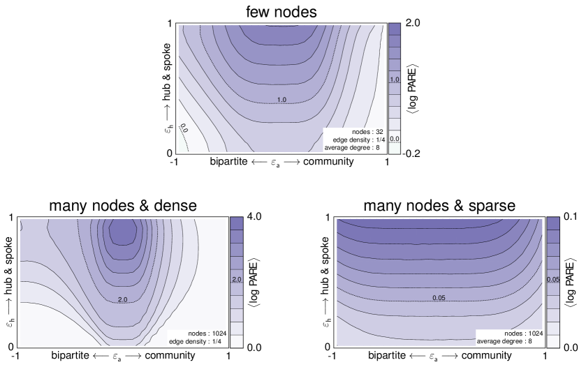
At this point, we estimate via Monte Carlo sampling, resulting in Figure 7.
A.3 The Results
Appendix B The Limit of Few Observed Graphs (Singular Covariance Estimates)
Below a certain number of observed graphs, the test using moments results in singular covariance matrices. If the sum of the two covariance matrices is also singular, one cannot take its inverse, so the Mahalanobis distance (Equation 4) is ill-defined. Here, we illustrate the simplest example: when there is only graph per sample, the distributions inferred by the test using moments have zero variance in the edge density .
Consider a single observed graph with nodes and edges. For the test using moments, the expected subgraph densities of the inferred distribution are taken to be those of this observed graph: . The estimation of the variance of assumes that the graph moments match to second order (and, as is fixed, their expected counts as well). At first order, we have
| (23) |
And at second order, we have
| (24) |
The only distributions satisfying both of these constraints are those containing graphs with precisely edges,666In Equations 23 and 24, we have edges instead of because we are considering (injective) homomorphism counts, which count both orientations of each edge. and thus the variance in edge density is zero: .
In a sense, this can be thought of as a covariance matrix of rank . In general, as the number of graphs per sample increases, the rank of the covariance matrix does as well. For a given order , one has covariance matrices of size (where is the number of connected subgraphs with edges), and therefore requires sufficiently many graphs per sample such that the rank of the sum of the two inferred covariance matrices is no less than . This is the reason behind the cutoff for the test using moments in Figure 5.
Appendix C Zero covariance between the edge density and the other graph cumulants for Erdős-Rényi distributions.
Theorem 1
For any Erdős-Rényi distribution , the covariance between the edge density and all other unbiased estimators of graph cumulants is zero.
Proof
We start by obtaining an expression for the covariance between the edge density777Recall that the edge density is both the first graph moment and the first graph cumulant, i.e.,
. and the moment of any subgraph ,
for graphs sampled
from an Erdős-Rényi distribution , where is the number of nodes in and is the i.i.d. probability of an edge between any pair of nodes.
Let denote the number of nodes in the subgraph , and its number of edges.
Recall that to compute the covariance between two subgraphs (Equation 11), one must consider all the ways that the nodes of the subgraphs could overlap (Section 7.2).
Here, there are four cases to consider:
-
1.
Neither node in the edge maps to any node in .
There is a single way this can happen, and it results in
a subgraph with nodes and edges. -
2.
A single node in the edge maps to a single node in .
There are ways this can happen, each resulting in
a subgraph with nodes and edges. -
3.
The two nodes of the edge map to two nodes in that do not already have an edge. There are ways this can happen, each resulting in
a subgraph with nodes and edges. -
4.
The two nodes of the edge map to two nodes in that already have an edge.
There are ways that this can happen, each resulting in
a subgraph with nodes and edges.
For an distribution, the moment of a subgraph is (i.e., to the power of the number of edges in ). Thus, the moments of the resulting subgraphs in cases 1, 2, and 3 are , while the moments of the resulting subgraphs in case 4 are . Moreover, recall that the injective homomorphism counts of a subgraph (with nodes) into a graph (with nodes) is , where the falling factorial is .
We now substitute these results into the expression for the covariance:
Using “algebra autopilot” and grouping the terms, we get:
| (25) |
Crucially, for an distribution, the covariance between the edge density and the density of a subgraph depends only on the number of edges in .
The is given by the sum of the covariances of the edge density with each subgraph that appears in the expression for the unbiased cumulant of (weighted by its coefficient in the formula). For example:
We now note two key facts about the expressions for the unbiased graph cumulants: 1) the subgraphs all have the same number of edges, and 2) the coefficients always sum to zero.
Hence, for any other subgraph ,
as desired.
References
- Aliakbarpour et al. (2018) Maryam Aliakbarpour, Amartya Shankha Biswas, Themis Gouleakis, John Peebles, Ronitt Rubinfeld, and Anak Yodpinyanee. Sublinear-time algorithms for counting star subgraphs via edge sampling. Algorithmica, 80(2):668–697, 2018.
- Alon (2007) Uri Alon. Network motifs: Theory and experimental approaches. Nature Review Genetics, 8(6):450–461, 2007.
- An (2016) Weihua An. Fitting ERGMs on big networks. Social Science Research, 59:107–119, 2016.
- Anderson (1958) Theodore Wilbur Anderson. An introduction to multivariate statistical analysis. Wiley, 1958.
- Asta and Shalizi (2014) Dena Asta and Cosma Rohilla Shalizi. Geometric network comparison. arXiv:1411.1350, 2014.
- Barabási and Albert (1999) Albert-László Barabási and Réka Albert. Emergence of scaling in random networks. Science, 286(5439):509–512, 1999.
- Bera et al. (2019) Suman K Bera, Noujan Pashanasangi, and C Seshadhri. Linear time subgraph counting, graph degeneracy, and the chasm at size six. arXiv:1911.05896, 2019.
- Bhattacharya et al. (2022) Bhaswar B Bhattacharya, Sayan Das, and Sumit Mukherjee. Motif estimation via subgraph sampling: The fourth-moment phenomenon. The Annals of Statistics, 50(2):987–1011, 2022.
- Bhattacharyya and Bickel (2015) Sharmodeep Bhattacharyya and Peter J Bickel. Subsampling bootstrap of count features of networks. The Annals of Statistics, 43(6):2384–2411, 2015.
- Bickel et al. (2011) Peter J Bickel, Aiyou Chen, and Elizaveta Levina. The method of moments and degree distributions for network models. The Annals of Statistics, 39(5):2280–2301, 2011.
- Biswas et al. (2020) Amartya Shankha Biswas, Talya Eden, Quanquan C Liu, Slobodan Mitrović, and Ronitt Rubinfeld. Massively parallel algorithms for small subgraph counting. arXiv:2002.08299, 2020.
- Borgs et al. (2008) Christian Borgs, Jennifer T Chayes, László Lovász, Vera T Sós, and Katalin Vesztergombi. Convergent sequences of dense graphs i: Subgraph frequencies, metric properties and testing. Advances in Mathematics, 219(6):1801–1851, 2008.
- Bravo-Hermsdorff and Gunderson (2019) Gecia Bravo-Hermsdorff and Lee M Gunderson. A unifying framework for spectrum-preserving graph sparsification and coarsening. Neural Information Processing Systems (NeurIPS), 33, 2019.
- Bressan (2021) Marco Bressan. Faster algorithms for counting subgraphs in sparse graphs. Algorithmica, 83(8):2578–2605, 2021.
- Casella and Berger (2021) George Casella and Roger L Berger. Statistical Inference. Cengage Learning, 2021.
- Chan et al. (2022) Stephanie CY Chan, Adam Santoro, Andrew K Lampinen, Jane X Wang, Aaditya Singh, Pierre H Richemond, Jay McClelland, and Felix Hill. Data distributional properties drive emergent few-shot learning in transformers. arXiv:2205.05055, 2022.
- Chen et al. (2020) Li Chen, Nathaniel Josephs, Lizhen Lin, Jie Zhou, and Eric D Kolaczyk. A spectral-based framework for hypothesis testing in populations of networks. arXiv:2011.12416, 2020.
- Chen et al. (2008) Yijia Chen, Marc Thurley, and Mark Weyer. Understanding the complexity of induced subgraph isomorphisms. In Automata, Languages and Programming: 35th International Colloquium (ICALP), pages 587–596. Springer, 2008.
- Chiba and Nishizeki (1985) Norishige Chiba and Takao Nishizeki. Arboricity and subgraph listing algorithms. SIAM Journal on Computing, 14(1):210–223, 1985.
- Dodeja et al. (2022) Vibhor Dodeja, Mohammad Almasri, Rakesh Nagi, Jinjun Xiong, and Wen-mei Hwu. PARSEC: Parallel subgraph enumeration in CUDA. In International Parallel and Distributed Processing Symposium (IPDPS), pages 168–178. IEEE, 2022.
- Gabbiani and Cox (2017) Fabrizio Gabbiani and Steven J Cox. Mathematics for neuroscientists. Academic Press, 2017.
- Gao and Lafferty (2017) Chao Gao and John Lafferty. Testing network structure using relations between small subgraph probabilities. arXiv:1704.06742, 2017.
- Ghoshdastidar et al. (2020) Debarghya Ghoshdastidar, Maurilio Gutzeit, Alexandra Carpentier, and Ulrike Von Luxburg. Two-sample hypothesis testing for inhomogeneous random graphs. The Annals of Statistics, 48(4):2208–2229, 2020.
- Ginoza and Mugler (2010) Reid Ginoza and Andrew Mugler. Network motifs come in sets: Correlations in the randomization process. Physics Review E, 82(1):011921, 2010.
- Gnedenko and Kolmogorov (1954) Boris V Gnedenko and Andrey Kolmogorov. Limit Distributions for Sums of Independent Random Variables. Addison-Wesley, 1954.
- Gui et al. (2019) Chuangyi Gui, Long Zheng, Pengcheng Yao, Xiaofei Liao, and Hai Jin. Fast triangle counting on GPU. In High Performance Extreme Computing Conference (HPEC), pages 1–7. IEEE, 2019.
- Gunderson and Bravo-Hermsdorff (2020) Lee M Gunderson and Gecia Bravo-Hermsdorff. Introducing graph cumulants: What is the variance of your social network? arXiv:2002.03959, 2020.
- Hald (2000) Anders Hald. The early history of the cumulants and the Gram-Charlier series. International Statistical Review, 68(2):137–153, 2000.
- Holland et al. (1983) Paul W Holland, Kathryn Blackmond Laskey, and Samuel Leinhardt. Stochastic blockmodels: First steps. Social Networks, 5(2):109–137, 1983.
- Hubel and Wiesel (1959) David H Hubel and Torsten N Wiesel. Receptive fields of single neurones in the cat’s striate cortex. The Journal of Physiology, 148(3):574, 1959.
- Jin et al. (2021) Jiashun Jin, Zheng Tracy Ke, and Shengming Luo. Optimal adaptivity of signed-polygon statistics for network testing. The Annals of Statistics, 49(6):3408–3433, 2021.
- Kardar (2007) Mehran Kardar. Statistical Physics of Particles. Cambridge University Press, 2007.
- Khan et al. (2018) Salman Khan, Hossein Rahmani, Syed Afaq Ali Shah, and Mohammed Bennamoun. A guide to convolutional neural networks for computer vision. Synthesis lectures on computer vision, 8(1):1–207, 2018.
- LeCun et al. (1998) Yann LeCun, Léon Bottou, Yoshua Bengio, and Patrick Haffner. Gradient-based learning applied to document recognition. Proceedings of the IEEE, 86(11):2278–2324, 1998.
- Lehner (2004) Franz Lehner. Cumulants in noncommutative probability theory I. Noncommutative exchangeability systems. Mathematische Zeitschrift, 248(1):67–100, 2004.
- Liu et al. (2020) Xin Liu, Haojie Pan, Mutian He, Yangqiu Song, Xin Jiang, and Lifeng Shang. Neural subgraph isomorphism counting. In Proceedings of the 26th ACM SIGKDD International Conference on Knowledge Discovery & Data Mining, pages 1959–1969, 2020.
- Lovász (2012) László Lovász. Large Networks and Graph Limits. American Mathematical Society, 2012.
- Lovász and Szegedy (2010) László Lovász and Balázs Szegedy. The graph theoretic moment problem. arXiv:1010.5159, 2010.
- Mahalanobis (1936) Prasanta Chandra Mahalanobis. On the generalized distance in statistics. In National Institute of Science of India, pages 49–55, 1936.
- Masuda et al. (2018) Naoki Masuda, Sadamori Kojaku, and Yukie Sano. Configuration model for correlation matrices preserving the node strength. Physical Review E, 98(1):012312, 2018.
- Maugis et al. (2016) PA Maugis, Sofia C Olhede, and Patrick J Wolfe. Fast counting of medium-sized rooted subgraphs. arXiv:1701.00177, 2016.
- Maugis et al. (2020) Pierre-André Maugis, Sofia C Olhede, Carey E Priebe, and Patrick J Wolfe. Testing for equivalence of network distribution using subgraph counts. Journal of Computational and Graphical Statistics, 29(3):455–465, 2020.
- McCullagh (1987) Peter McCullagh. Tensor Methods in Statistics: Monographs on Statistics and Applied Probability. Chapman and Hall, 1987.
- Mukherjee et al. (2016) Soumendu Sundar Mukherjee, Purnamrita Sarkar, and Lizhen Lin. On clustering network-valued data. arXiv:1606.02401, 2016.
- Newman (2001) Mark EJ Newman. The structure of scientific collaboration networks. Proceedings of the National Academy of Sciences, 98(2):404–409, 2001.
- Orbanz (2017) Peter Orbanz. Subsampling large graphs and invariance in networks. arXiv:1710.04217, 2017.
- Ouyang et al. (2019) Guang Ouyang, Dipak K Dey, and Panpan Zhang. Clique-based method for social network clustering. Journal of Classification, 37(1):1–21, 2019.
- Pattillo et al. (2013) Jeffrey Pattillo, Nataly Youssef, and Sergiy Butenko. On clique relaxation models in network analysis. European Journal of Operational Research, 226(1):9–18, 2013.
- Persson et al. (2021) Emma Persson, Miguel Castresana-Aguirre, Davide Buzzao, Dimitri Guala, and Erik L.L. Sonnhammer. FunCoup 5: Functional association networks in all domains of life, supporting directed links and tissue-specificity. Journal of Molecular Biology, 433(11):166835, 2021.
- Pinar et al. (2017) Ali Pinar, C Seshadhri, and Vaidyanathan Vishal. Escape: Efficiently counting all 5-vertex subgraphs. In Proceedings of the 26th International Conference on World Wide Web, pages 1431–1440, 2017.
- Pitman (1949) Edwin JG Pitman. Notes on non-parametric statistical inference. Technical report, North Carolina State University, Department of Statistics, 1949.
- Rao (1992) C Radhakrishna Rao. Information and the accuracy attainable in the estimation of statistical parameters. In Breakthroughs in Statistics, pages 235–247. Springer, 1992.
- Rauh (2017) Johannes Rauh. The polytope of -star densities. The Electronic Journal of Combinatorics, pages 1–4, 2017.
- Reiser (2001) Benjamin Reiser. Confidence intervals for the Mahalanobis distance. Communications in Statistics-Simulation and Computation, 30(1):37–45, 2001.
- Ribeiro et al. (2021) Pedro Ribeiro, Pedro Paredes, Miguel EP Silva, David Aparicio, and Fernando Silva. A survey on subgraph counting: concepts, algorithms, and applications to network motifs and graphlets. ACM Computing Surveys (CSUR), 54(2):1–36, 2021.
- Rota and Shen (2000) Gian-Carlo Rota and Jianhong Shen. On the combinatorics of cumulants. Journal of Combinatorial Theory, Series A, 91:283–304, 2000.
- Stuart and Kendall (1963) Alan Stuart and Maurice G Kendall. The Advanced Theory of Statistics. Charles Griffin and Co., Ltd., London, 1963.
- Tang et al. (2017) Minh Tang, Avanti Athreya, Daniel L Sussman, Vince Lyzinski, Youngser Park, and Carey E Priebe. A semiparametric two-sample hypothesis testing problem for random graphs. Journal of Computational and Graphical Statistics, 26(2):344–354, 2017.
- Tantardini et al. (2019) Mattia Tantardini, Francesca Ieva, Lucia Tajoli, and Carlo Piccardi. Comparing methods for comparing networks. Scientific Reports, 9(1):1–19, 2019.
- Vaswani et al. (2017) Ashish Vaswani, Noam Shazeer, Niki Parmar, Jakob Uszkoreit, Llion Jones, Aidan N Gomez, Łukasz Kaiser, and Illia Polosukhin. Attention is all you need. Neural Information Processing Systems (NIPS), 30, 2017.
- Xia et al. (2019) Feng Xia, Haoran Wei, Shuo Yu, Da Zhang, and Bo Xu. A survey of measures for network motifs. IEEE Access, 7:106576–106587, 2019.
- Ye et al. (2022) Xiaowei Ye, Rong-Hua Li, Qiangqiang Dai, Hongzhi Chen, and Guoren Wang. Lightning fast and space efficient k-clique counting. In Proceedings of the ACM Web Conference 2022, pages 1191–1202, 2022.
- Zhang and Xia (2022) Yuan Zhang and Dong Xia. Edgeworth expansions for network moments. The Annals of Statistics, 50(2):726–753, 2022.
- Zhao et al. (2021) Kangfei Zhao, Jeffrey Xu Yu, Hao Zhang, Qiyan Li, and Yu Rong. A learned sketch for subgraph counting. In International Conference on Management of Data, pages 2142–2155, 2021.