Artificial Neural Networks for Galaxy Clustering:
Learning from the two-point correlation function of BOSS galaxies

Abstract

The increasingly large amount of cosmological data coming from ground-based and space-borne telescopes requires highly efficient and fast enough data analysis techniques to maximise the scientific exploitation. In this work, we explore the capabilities of supervised machine learning algorithms to learn the properties of the large-scale structure of the Universe, aiming at constraining the matter density parameter, $\Omega_{m}$. We implement a new Artificial Neural Network for a regression data analysis, and train it on a large set of galaxy two-point correlation functions in standard cosmologies with different values of $\Omega_{m}$. The training set is constructed from log-normal mock catalogues which reproduce the clustering of the Baryon Oscillation Spectroscopic Survey (BOSS) galaxies. The presented statistical method requires no specific analytical model to construct the likelihood function, and runs with negligible computational cost, after training. We test this new Artificial Neural Network on real BOSS data, finding $\Omega_{m}=0.309\pm 0.008$, which is consistent with standard analysis results.

language=C++, backgroundcolor=, basicstyle=, commentstyle=, classoffset=1, morekeywords=cosmobl, DirCosmo, DirLoc, Cosmology, par, Object, Galaxy, Catalogue, random_catalogue_box, TwoPointCorrelation, keywordstyle=, classoffset=2, morekeywords=fsigma8, nObjects, setParameters, measure_xi, write_xi, keywordstyle=, classoffset=0, tabsize=2, captionpos=b, frame=lines, frameround=fttt, numbers=left, numberstyle=, numbersep=5pt, breaklines=true, showstringspaces=false language=Python, backgroundcolor=, basicstyle=, commentstyle=, classoffset=1, morekeywords=Cosmology, pyCosmologyCBL, keywordstyle=, classoffset=2, morekeywords=D_C, keywordstyle=, classoffset=0, tabsize=2, captionpos=b, frame=lines, numbers=left, numberstyle=, numbersep=5pt, breaklines=true, showstringspaces=false, procnamekeys=def,class

1 Introduction

One of the biggest challenges of modern cosmology is to accurately estimate the standard cosmological model parameters and, possibly, to discriminate among alternative cosmological frameworks. Fast and accurate statistical methods are required to maximise the scientific exploitation of the cosmological probes of the large-scale structure of the Universe. During the last decades, increasingly large surveys have been conducted both with ground-based and space-borne telescopes, and a huge amount of data is expected from next-generation projects, like e.g. Euclid (Laureijs et al., 2011; Blanchard et al., 2020) and the Vera C. Rubin Observatory (LSST Dark Energy Science Collaboration, 2012). This scenario, in which the amount of available data is expected to keep growing with exponential rate, suggests that machine learning techniques shall play a key role in cosmological data analysis, due to the fact that their reliability and precision strongly depend on the quantity and variety of inputs they are given.

According to the standard cosmological scenario, the evolution of density perturbations started from an almost Gaussian distribution, primarily described by its variance. In configuration space, the variance of the field is the two-point correlation function (2PCF), which is a function of the magnitude of the comoving distance between objects, $r$. At large enough scales, the matter distribution can still be approximated as Gaussian, and thus the 2PCF contains most of the information of the density field.

The 2PCF and its analogous in Fourier space, the power spectrum, have been the focus of several cosmological analyses of observed catalogues of extra-galactic sources (see e.g. Totsuji and Kihara, 1969; Peebles, 1974; Hawkins et al., 2003; Parkinson et al., 2012; Bel et al., 2014; Alam et al., 2016; Pezzotta et al., 2017; Mohammad et al., 2018; Gil-Marín et al., 2020; Marulli et al., 2021, and references therein). The standard way to infer constraints on cosmological parameters from the measured 2PCF is by comparison with a physically motivated model through an analytical likelihood function. The latter should account for all possible observational effects, including both statistical and systematic uncertainties. In this work, we investigate an alternative data analysis method, based on a supervised machine learning technique, which does not require a customized likelihood function to model the 2PCF. Specifically, the 2PCF shape will be modelled with an Artificial Neural Network (NN), trained on a sufficiently large set of measurements from mock data sets generated at different cosmologies.

Supervised machine learning methods can be considered as a complementary approach to standard data analysis techniques for the investigation of the large-scale structure of the Universe. There are two main issues in applying machine learning algorithms in this context. Firstly, the simulated galaxy maps used to train the NNs have to be sufficiently accurate at all scales of interest, including all the relevant observational effects characterizing the surveys to be analysed. Indeed, the NN outputs rely only on the examples provided for the training phase, and not according to any specific instructions (Samuel, 1959; Goodfellow et al., 2016). The accuracy of the output depends on the level of reliability of the training set, while the precision increases when the amount of training data set increases. Moreover, significant computational resources are required to construct the mock data sets in a high enough number of test cosmologies.

On the other hand, both the construction of the mock data sets and the NN training and validation have to be done only once. After that, the NN can produce outputs with negligible computational cost, and can exploit all physical scales on which the mock data sets are reliable, that is possibly beyond the domain in which an analytic likelihood is available. These represent the key advantages of this novel, complementary data analysis technique.

Machine learning based methods should provide an effective tool in cosmological investigations based on increasingly large amounts of cosmological data from extra-galactic surveys (e.g. Cole et al., 2005; Parkinson et al., 2012; Anderson et al., 2014; Kern et al., 2017; Ntampaka et al., 2019; Ishida, 2019; Hassan et al., 2020; Villaescusa-Navarro, 2021). In fact, these techniques have already been exploited for the analysis of the large-scale structure of the Universe (see e.g. Aragon-Calvo, 2019; Tsizh et al., 2020). In some cases, machine learning models have been trained and tested on simulated mock catalogues to obtain as output the cosmological parameters those simulations had been constructed with (e.g. Ravanbakhsh et al., 2016; Pan et al., 2020). These works demonstrated that the machine learning approach is powerful enough to infer tight constraints on cosmological model parameters, when the training set is the distribution of matter in a three-dimensional grid.

The method we are presenting in this work is different in this respect, as our input training set consists of 2PCF measurements estimated from mock galaxy catalogues. The rationale of this choice is to help the network to efficiently learn the mapping between the cosmological model and the corresponding galaxy catalogue by exploiting the information compression provided by the second-order statistics of the density field. The goal of this work is to implement, train, validate and test a new NN of this kind, and to investigate its capability in providing constraints on the matter density parameter, $\Omega_{m}$, from real galaxy clustering data sets.

The construction of proper training samples would require running N-body or hydrodynamic simulations in a sufficiently large set of cosmological scenarios. As already noted, this task demands substantial computational resources and a dedicated work, which is beyond the scope of the current analysis. A forthcoming paper will be dedicated to this fundamental task. Here instead we rely on log-normal mock catalogues, which can reproduce the monopole of the redshift-space 2PCF of real galaxy catalogues with reasonable accuracy and in a minimal amount of time. This will allow us to test our NN on training data sets with the desired format, in order to be ready for forthcoming analyses with more reliable data sets. Moreover, future developments of the presented method will involve estimating a higher number of cosmological parameters at the same time. The implemented NN is provided through a public Google Colab notebook.

The paper is organised as follows. In Section 2 we give a general overview of the data analysis method we present in this work. In Section 3 we describe in detail the characteristics of the catalogues used to train, validate and test the NN. The specifics on the NN itself, together with its results on the test set of mock catalogues are described in Section 4. The application to the BOSS galaxy catalogue and the results this leads to are presented in Section 5. In Section 6 we draw our conclusions and discuss about possible future improvements. Finally, A provides details on the algorithms used to construct the log-normal mock catalogues.

2 The data analysis method

The data analysis method considered in this work exploits a supervised machine learning approach. Our general goal is to extract cosmological constraints from extra-galactic redshift surveys with properly trained NNs. As a first application of this method, we focus the current analysis on the 2PCF of BOSS galaxies, which is exploited to extract constraints on $\Omega_{m}$.

The method consists of a few steps. Firstly, a fast enough process to construct the data sets with which train, validate and test the NN is needed. In this work we train the NN with a set of 2PCF mock measurements obtained from log-normal catalogues. The construction of these input data sets is described in detail in Section 3. Specifically, we create several sets of mock BOSS-like catalogues assuming as values for the cosmological parameters the ones inferred from the Planck Cosmic Microwave Background observations, except for $\Omega_{m}$, that assumes different values in different mock catalogues, and $\Omega_{\Lambda}$ that has been changed every time in order to have $\Omega_{tot}=\Omega_{m}+\Omega_{\Lambda}+\Omega_{rad}=1$, where $\Omega_{\Lambda}$ and $\Omega_{rad}$ are the dark energy and the radiation density parameters, respectively. Specifically, we fix the main parameters of the $\Lambda$-cold dark matter ($\Lambda$CDM) model to the following values: $\Omega_{b}\,h^{2}=0.02237$, $\Omega_{c}\,h^{2}=0.1200$, $100\,\Theta_{MC}=1.04092$, $\tau=0.0544$, $\textrm{ln}(10^{10}\,A_{s})=3.044$, and $n_{s}=0.9649$ (Aghanim et al., 2018, Table 2, TT,TE+lowE+lensing). Here $h$ indicates one hundredth of the Hubble constant, $H_{0}$.

The implemented NN performs a regression analysis, that is it can assume every value within the range the algorithm has been trained for, that in our case is $0.24<\Omega_{m}<0.38$. In particular, the algorithm takes as input a 2PCF monopole measurement, and provides as output a Gaussian probability distribution on $\Omega_{m}$, from which we can extract the mean and standard deviation (see Section 3.4 and A). Specifically, the data sets used for training, validating and testing the NN consist of different sets of 2PCF monopole measures, labelled by the value of $\Omega_{m}$ assumed to construct the mock catalogues these measures have been obtained from, and assumed also during the measure itself.

After the training and validation phases, we test the NN with a set of input data sets constructed with random values of $\Omega_{m}$, that is, different values from the ones considered in the training and validation sets. The structure of the NN, the characteristics of the different sets of data it has been fed with, and how the training process of the NN has been led are described in Section 4.

Finally, once the NN has proven to perform correctly on a test set of 2PCF measures from the BOSS log-normal mock catalogues, we exploit it on the real 2PCF of the BOSS catalogue. To measure the latter sample statistic, a cosmological model has to be assumed, which leads to geometric distortions when the assumed cosmology is different to the true one. To test the impact of these distortions on our final outcomes, we repeat the analysis measuring the BOSS 2PCF assuming different values of $\Omega_{m}$. We find that our NN provides in output statistically consistent results independently of the assumed cosmology. The results of this analysis are described in detail in Section 5.

We provide below a summary of the main steps of the data analysis method investigated in this work:

1. Assume a cosmological model. In the current analysis, we assume a value of $\Omega_{m}$, and fix all the other main parameters of the $\Lambda$CDM cosmological model to the Planck values. A more extended analysis is planned for a forthcoming work.

2. Measure the 2PCF of the real catalogue to be analysed and use it to estimate the large-scale galaxy bias. This is required to construct mock galaxy catalogues with the same clustering amplitude of the real data. Here we estimate the bias from the redshift-space monopole of the 2PCF at large scales (see Section 3.3).

3. Construct a sufficiently large set of mock catalogues. In this work we consider log-normal mock catalogues, that can be obtained with fast enough algorithms. The measured 2PCFs of these catalogues will be used for the training, the validation and the test of the NN.

4. Repeat all the above steps assuming different cosmological models. Different cosmological models, characterised by different values of $\Omega_{m}$, are assumed to create different classes of mock catalogues and measure the 2PCF of BOSS galaxies.

5. Train and validate the NN.

6. Test the NN. This has to be done with data sets constructed considering cosmological models not used for the training and validation, to check whether the model can make reliable predictions also on previously unseen examples.

7. Exploit the trained NN on real 2PCF measurements. This is done feeding the trained machine learning model with the several measures of the 2PCF of the real catalogue, obtained assuming different cosmological models. The reason for this is to check whether the output of the NN is affected by geometric distortions.

3 Creation of the data set

3.1 The BOSS data set

The mock catalogues used for the training, validation and test of our NN are constructed to reproduce the clustering of the BOSS galaxies. BOSS is part of the Sloan Digital Sky Survey (SDSS), which is an imaging and spectroscopic redshift survey that used a $2.5$m modified Ritchey-Chrétien altitude-azimuth optical telescope located at the Apache Point Observatory in New Mexico (Gunn et al., 2006). The data we have worked on are from the Data Release 12 (DR12), that is the final data release of the third phase of the survey (SDSS-III) (Alam et al., 2015). The observations were performed from fall 2009 to spring 2014, with a 1000-fiber spectrograph at a resolution $R\approx 2000$. The wavelength range goes from $360$ nm to $1000$ nm, and the coverage of the survey is $9329$ square degrees.

The catalogue from BOSS DR12, used in this work, contains the positions in observed coordinates (RA, Dec and redshift) of $1\,198\,004$ galaxies up to redshift $z=0.8$.

Both the data and the random catalogues are created considering the survey footprint, veto masks and systematics of the survey, as e.g. fiber collisions and redshift failures. The method used to construct the random catalogue from the BOSS spectroscopic observations is detailed in Reid et al. (2016).

3.2 Two-point correlation function estimation

We estimate the 2PCF monopole of the BOSS and mock galaxy catalogues with the Landy and Szalay (1993) estimator:

$$\xi(s)=1+\frac{N_{\rm RR}}{N_{\rm DD}}\frac{DD(s)}{RR(s)}-2\frac{N_{\rm RR}}{N_{\rm DR}}\frac{DR(s)}{RR(s)}\;,$$ (1)

where $DD(s)$, $RR(s)$ and $DR(s)$ are the number of galaxy-galaxy, random-random and galaxy-random pairs, within given comoving separation bins (i.e. in $s\pm\Delta s$), respectively, while $N_{\rm DD}=N_{D}(N_{D}-1)/2$, $N_{\rm RR}=N_{R}(N_{R}-1)/2$ and $N_{\rm DR}=N_{D}N_{R}$ are the corresponding total number of galaxy-galaxy, random-random and galaxy-random pairs, being $N_{D}$ and $N_{R}$ the number of objects in the real and random catalogues. The random catalogue is constructed with the same angular and redshift selection functions of the BOSS catalogue, but with a number of objects that is ten times bigger than the observed one, to minimise the impact of Poisson errors in random pair counts.

3.3 Galaxy bias

As introduced in the previous Sections, we train our NN to learn the mapping between the 2PCF monopole shape, $\xi$, and the matter density parameter, $\Omega_{m}$. Thus, we construct log-normal mock catalogues assuming different values of $\Omega_{m}$. A detailed description of the algorithm used to construct these log-normal mocks is provided in the next Section 3.4.

Firstly, we need to estimate the bias of the objects in the sample, $b$. We consider a linear bias model, whose bias value is estimated from the data. Specifically, when a new set of mock catalogues (characterised by $\Omega_{m}=\Omega_{m,i}$) is constructed, a new linear galaxy bias has to be estimated. The galaxy bias is assessed by modelling the 2PCF of BOSS galaxies in the scale range $30<s\,[h^{-1}\,\mbox{Mpc}]<50$, where $s$ is used here, instead of $r$, to indicate separations in redshift space. We consider a Gaussian likelihood function, assuming a Poissonian covariance matrix which is sufficiently accurate for the purposes of this work. We model the shape of the redshift-space 2PCF at large scale as follows (Kaiser, 1987):

$$\xi_{\rm gal}(s)=\left[(b\sigma_{8})^{2}+\frac{2}{3}f\sigma_{8}+\frac{1}{5}(f\sigma_{8})^{2}\right]\frac{1}{\sigma_{8}^{2}}\xi_{m}(r)\;,$$ (2)

where the matter 2PCF, $\xi_{m}(r)$, is obtained by Fourier transforming the matter power spectrum modelled with the Code for Anisotropies in the Microwave Background (CAMB) (Lewis et al., 2000). The product between the linear growth rate and the matter power spectrum normalisation parameter, $f\sigma_{8}$, is set by the cosmological model assumed during the measuring of the 2PCF and the construction of the theoretical model. The values of all redshift-dependent parameters have been calculated using the mean redshift of the data catalogue, $z=0.481$.

We assume a uniform prior for $b\sigma_{8}$ between $0$ and $2.7$. The posterior has been sampled with a Markov Chain Monte Carlo algorithm with $10\,000$ steps and a burn-in period of $100$ steps. The linear bias, $b$, is then derived by dividing the posterior median by $\sigma_{8}$. The latter is estimated from the matter power spectrum computed assuming Planck cosmology. We note that this method implies that only the shape of the 2PCF is actually used to constrain $\Omega_{m}$.

3.4 Mock galaxy catalogues

As described in Section 2, the data sets used for the training, validation and test of the NN implemented in this work consist of 2PCF mock measurements estimated from log-normal galaxy catalogues. Log-normal mock catalogues are generally used to create the data set necessary for the covariance matrix estimate, in particular in anisotropic clustering analyses (see e.g. Lippich et al., 2019). In fact, this technique allows us to construct density fields and, thus, galaxy catalogues with the required characteristics in an extremely fast way, especially if compared to N-body simulations, though the latter are more reliable at higher-order statistics and in the fully nonlinear regime.

To construct the log-normal mock catalogues, we adopted the same strategy followed by Beutler et al. (2011). We provide here a brief explanation of the method, while a more detailed description is given in A. As already commented in Section 1, log-normal catalogues do not provide the optimal training sets for this machine learning method, but are used here only to test the algorithms with input data with the desired format.

The algorithm used in this work to generate these mock catalogues for the machine learning training process takes as input one data catalogue and one corresponding random catalogue. These are used to define a grid with the same geometric structure of the data catalogue and a visibility mask function which is constructed from the pixel density of the random catalogue. A cosmological model has to be assumed to compute the object comoving distances from the observed redshifts and to model the matter power spectrum. The latter is used to estimate the galaxy power spectrum, which is the logarithm of the variance of the log-normal random field.

The density field is then sampled from this random field. Specifically, once the algorithm has associated to all the grid cells their density value, we can extract from each of them a certain number of points that depend on the density of the catalogue and on the visibility function. These points represent the galaxies of the output mock catalogue.

Once the mocks are created, the same cosmological model is assumed also to measure the 2PCF. We repeated the same process for all the test values of $\Omega_{m}$. That is, for each $\Omega_{m}$ we created a set of log-normal mock catalogues and measured the 2PCF. This is different with respect to standard analyses, where a cosmology is assumed only once for the clustering measurements, and geometric distortions are included in the likelihood.

As an illustrative example, Figure 1 shows different measures of the 2PCF obtained in the scale range $8<s\,[h^{-1}\,\mbox{Mpc}]<50$, in $30$ logarithmic bins of $s$, and assuming the lowest and the highest values of $\Omega_{m}$ that have been considered in this work, that are $\Omega_{m}=0.24$ and $\Omega_{m}=0.38$. The black and red dots show the measures obtained from the corresponding two sets of $50$ log-normal mock galaxy catalogues, while the dashed lines are the theoretical 2PCF models assumed to construct them. As expected, the average 2PCFs of the two sets of log-normal catalogues are fully consistent with the corresponding theoretical predictions. Indeed, a mock log-normal catalogue characterised by $\Omega_{m}=\Omega_{m,i}$ provides a training example for the NN describing how galaxies would be distributed if $\Omega_{m,i}$ was the true value. Finally, the blue and green squares show the 2PCFs of the real BOSS catalogue obtained by assuming $\Omega_{m}=0.24$ and $\Omega_{m}=0.38$, respectively, when converting galaxy redshifts into comoving coordinates. The differences in the latter two measures are caused by geometric distortions. As can be seen, neither of these two data sets are consistent with the corresponding 2PCF theoretical models, that is both $\Omega_{m}=0.24$ and $\Omega_{m}=0.38$ appear to be bad guesses for the real value of $\Omega_{m}$. As we will show in Section 5, the NN presented in this work is not significantly affected by geometric distortions.

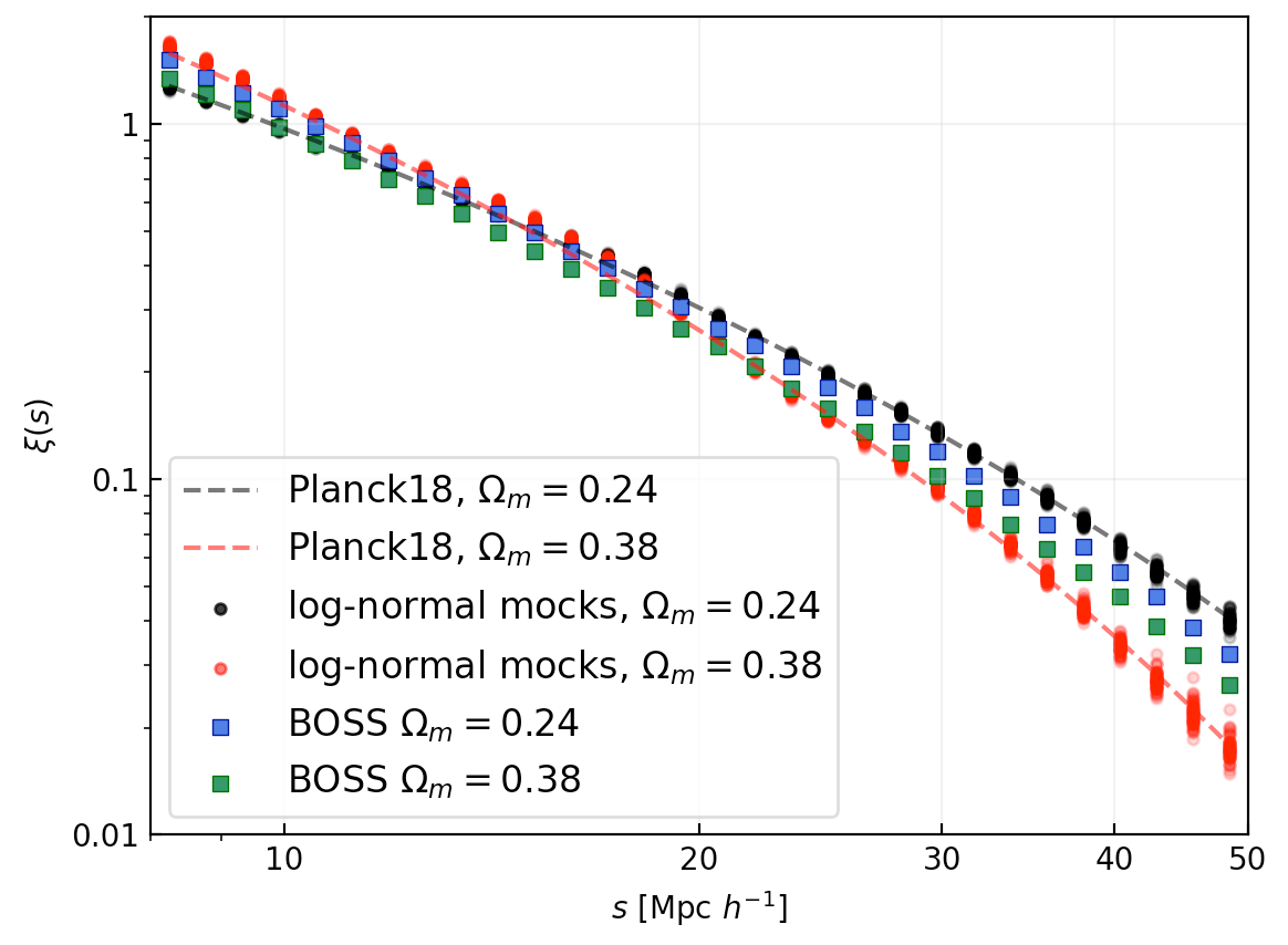
Figure 1: Different measures of the 2PCF monopole. The dots represent the measures obtained from $50$ log-normal mock catalogues constructed with $\Omega_{m}=0.24$ (black dots) and $\Omega_{m}=0.38$ (red dots). The black and red dashed lines show the corresponding theoretical 2PCF models. The blue and green squares show the real BOSS 2PCFs measured assuming the same cosmologies of the mock catalogues, that is $\Omega_{m}=0.24$ and $\Omega_{m}=0.38$, respectively, when converting redshifts into comoving coordinates.

4 The Artificial Neural Network

4.1 Architecture

Regression machine learning models take as input a set of variables that can assume every value and provide as output a continuous value. In our case, the input data set is a 2PCF measure, while the output is the predicted Gaussian probability distribution of $\Omega_{m}$. Specifically, the regression model we are about to describe has been trained with 2PCF measures in the scale range $8-50h^{-1}\,\mbox{Mpc}$, in $30$ logarithmic scale bins.

The architecture of the implemented NN is schematically represented in Figure 2. It consists of the following layers:

• Input layer that feeds the $30$ values of the measured 2PCF to the model;

• Dense layer with 2 units. Every unit of this layer performs the following linear operation on the input elements:

  $$y=\sum_{i}w_{i}\cdot x_{i}+b\ \ ,$$ (3)

  where $y$ is the output of the unit, $x_{i}$ is the $i$-th element of the input, $w_{i}$ is its corresponding weight, and $b$ is the intercept of the linear operation. No nonlinear activation function has been used in this layer. This choice has been proven to be convenient a posteriori, providing excellent performance of the NN during the test phase (see Section 4.3). We thus decided not to introduce any activation function to keep the architecture of the regression model as simple as possible;

• Distribution layer that uses the two outputs of the dense layer as mean and standard deviation to parameterise a Gaussian distribution, which is given as output.

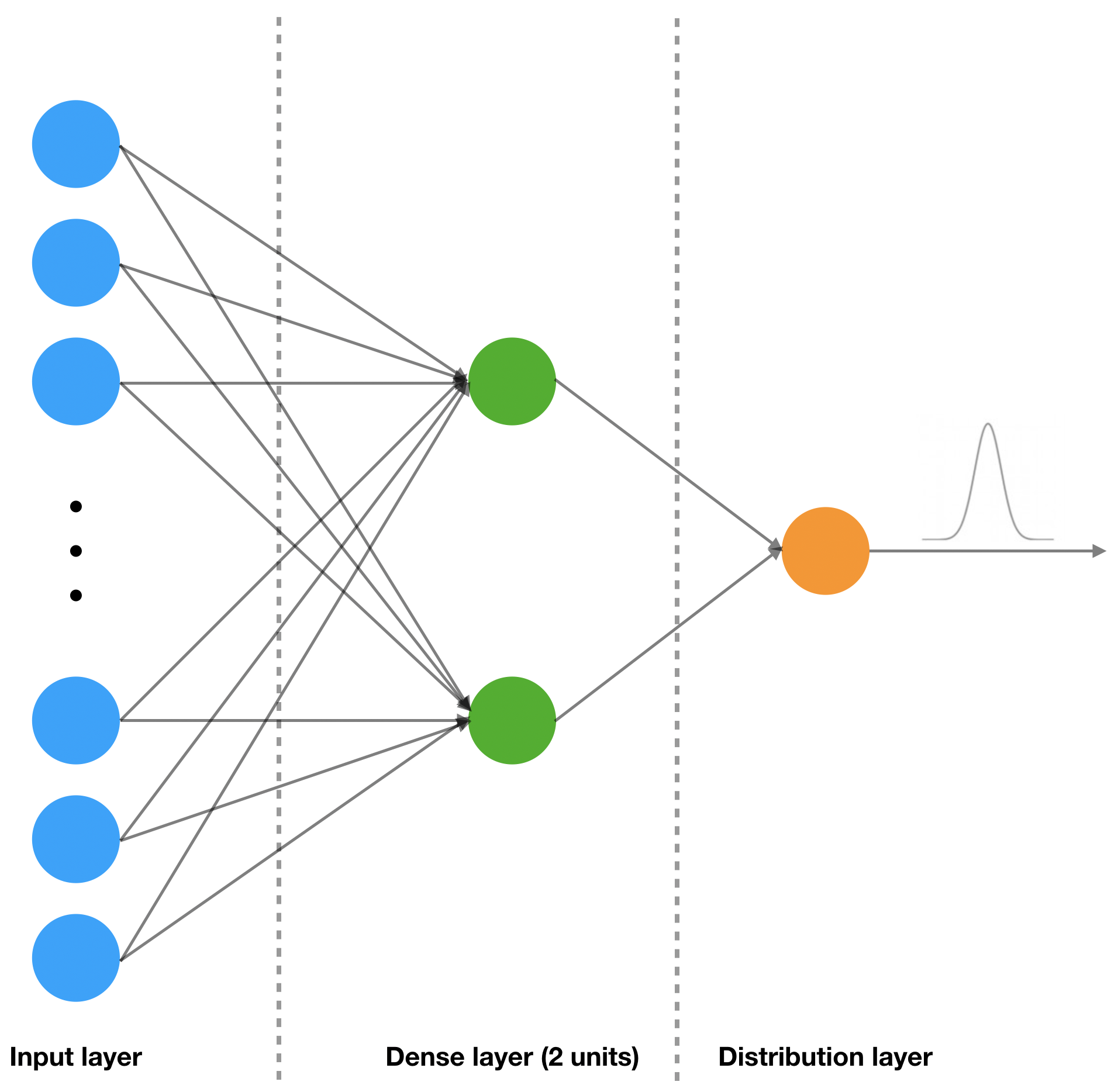
Figure 2: Schematic representation of the regression model considered in this work. The input layer is represented by blue dots, the hidden dense layer by green dots, and the output layer by the orange dot.

This architecture has been chosen because it is the simplest one we tested which is able to provide accurate cosmological constraints. Deeper models have been tried out, but no significant differences were spotted in the output predictions.

4.2 Training and validation

The training and validation sets are constructed separately, and consist of $2\,000$ and $800$ examples, respectively. Regression machine learning models work better if the range of possible outputs is well represented in the training and validation sets. We construct mock catalogues with $40$ different values of $\Omega_{m}$: $29$ from $\Omega_{m}=0.24$ to $\Omega_{m}=0.38$ with $\Delta\Omega_{m}=0.005$ and $11$ from $\Omega_{m}=0.2825$ to $\Omega_{m}=0.3325$, also separated by $\Delta\Omega_{m}=0.005$. The latter are added to improve the density of inputs in the region that had proven to be the one where the predictions were more likely, during the first attempts of the NN training. The training and validation sets consist of $50$ and $20$ 2PCF measures for each value of $\Omega_{m}$, respectively. All the mock catalogues used for the training and validation have the same dimension of the BOSS 2PCF measures.

The loss function used for the training process is the following:

$$J=-\sum_{i=1}^{N}\log\left[\frac{1}{\sqrt{2\pi}\sigma_{i}}\exp{-\frac{(l_{i}-\mu_{i})^{2}}{2\sigma_{i}^{2}}}\right]\;,$$ (4)

where $N$ is the number of examples, $l_{i}$ is the label correspondent to the $i$-th 2PCF used for the training or the validation (i.e. the true value of $\Omega_{m}$ that has been used to create the $i$-th mock catalogue and to measure its 2PCF), while $\sigma_{i}$ and $\mu_{i}$ are the standard deviation and the mean of the Normal probability distribution function that is given as output for the same $i$-th 2PCF example.

During the training process, we apply the Adam optimisation (see Kingma and Ba, 2014, for a detailed description of its functioning and parameters) with the following three different steps:

• 750 epochs with $\eta=0.002$ ,

• 150 epochs with $\eta=0.001$ ,

• 100 epochs with $\eta=0.0005$ ,

where $\eta$ indicates the learning rate. During the three steps, the values of the other two parameters of this optimisation algorithm are kept fixed to $\beta_{1}=0.9$ and $\beta_{2}=0.999$, and the training set was not divided into batches. Variations in the parameters of the optimization have been performed and did not lead to significantly different outputs.

Gradually reducing the learning rate during the training helps the model to find the correct global minimum of the loss function (Ntampaka et al., 2019). The first epochs, having a higher learning rate, lead the model towards the area surrounding the global minimum, while the last ones, having a lower learning rate, and therefore being able to take smaller and more precise steps in the parameter space, have the task to lead the model towards the bottom of that minimum. In this model, minimizing the loss function means both to drive the mean values of the output Gaussian distributions towards the values of the labels (i.e. the values of $\Omega_{m}$ corresponding to the inputs), and to reduce as much as possible the standard deviation of those distributions.

During the training process, the interval of the labels, that is $0.24\leq\Omega_{m}\leq 0.38$, has been mapped into $[0,1]$ through the following linear operation:

$$L=\frac{l-0.24}{0.14}\;,$$ (5)

where $l$ is the original label and $L$ is the one that belongs to the $[0,1]$ interval. Once the mean, $\mu_{L}$, and the standard deviation, $\sigma_{L}$, of the predictions are obtained in output, we convert them back to match the original interval of the labels. The standard deviation is then computed as follows:

$$\frac{d\mu_{L}}{d\sigma_{L}}=\frac{d\mu_{l}}{d\sigma_{l}}\;,$$ (6)

where $\sigma$ is the standard deviation of $\mu$, so that the uncertainty on $\mu$ is given by $0.14\,\sigma_{L}$.

4.3 Test

The test set consists of $5$ different 2PCF measures obtained from log-normal mock catalogues with $16$ different randomly generated values of $\Omega_{m}$. Therefore, we have a total of $80$ measures. The $\Omega_{m}$ predictions and uncertainties are estimated as the mean and standard deviation of the Gaussian distributions obtained in output (Matthies, 2007; Der Kiureghian and Ditlevsen, 2009; Kendall and Gal, 2017; Russell and Reale, 2019). Our model is thus able to associate to every point of the input space an uncertainty on the output that depends on the intrinsic scatter of the 2PCF measures.

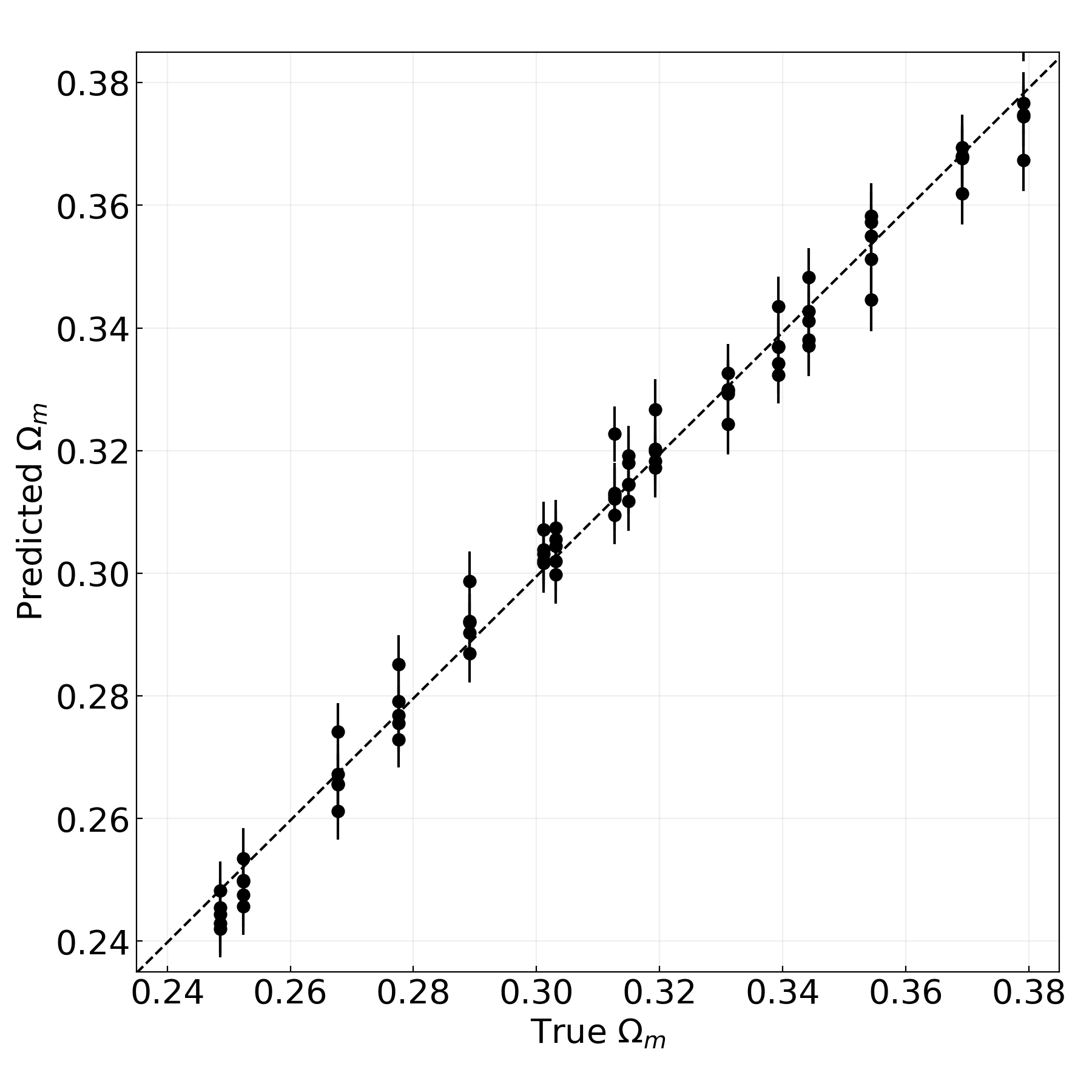
Figure 3: Values of $\Omega_{m}$ and related uncertainties predicted by our NN, compared with the best-fit linear model (dashed line). The best-fit slope is $0.995\pm 0.014$, while the best-fit normalisation is $0.001\pm 0.005$. The error bars in this plot represent the standard deviations of the distributions for $\Omega_{m}$ obtained as output of the NN

Figure 3 shows the predictions on the test set, compared to the true values of $\Omega_{m}$ the mocks in the test were constructed with. As can be seen, the implemented NN is able to provide reliable predictions when fed with measures from mock catalogues characterised by $\Omega_{m}$ values that were not used during the training and validation phases. In fact, fitting this data set with a linear model:

$$\Omega_{m}^{\rm pred}=\alpha\cdot\Omega_{m}^{\rm true}+\beta\;,$$ (7)

we get $\alpha=0.995\pm 0.014$ and $\beta=0.001\pm 0.005$, which are consistent with the slope and the intercept of the bisector of the quadrant. Figure 3 also shows that the estimates near the limits of the training range at $\Omega_{m}=0.24$ and $0.38$ are not biased, as the predictions on the test set, also for the most external examples, are consistent with the bisector of the quadrant.

5 Application to BOSS data

After training, validating and testing the NN, we can finally apply it to the real 2PCF of the BOSS galaxy catalogue. To test the impact of geometric distortions caused by the assumption of a particular cosmology during the measure, we apply the NN on $40$ measures of the 2PCF of BOSS galaxies obtained with different assumptions on the value of $\Omega_{m}$ when converting from observed to comoving coordinates.

Figure 4 shows the results of this analysis, compared with the $\Omega_{m}$ constraints provided by Alam et al. (2017).

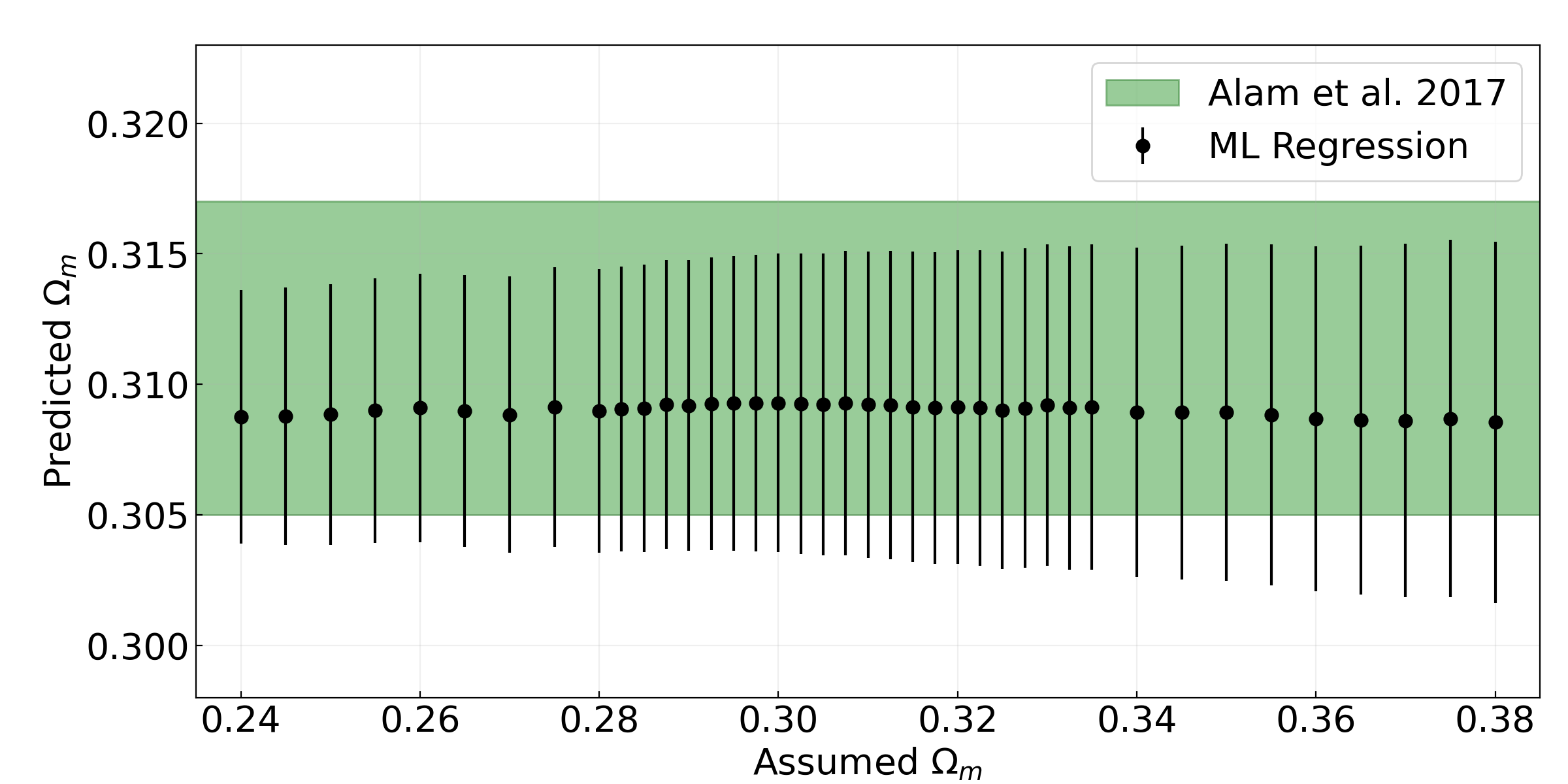
Figure 4: Machine learning predictions (black dots and bars) on $\Omega_{m}$ from the measured 2PCF of BOSS galaxies, as a function of the $\Omega_{m}$ assumed in the measurements. The predictions are compared to the $\Omega_{m}$ constraints provided by Alam et al. (2017), here represented by the green stripe.

The predictions of the NN have been fitted with a linear model:

$$\Omega_{m}^{\rm pred}=\alpha\cdot\Omega_{m}^{\rm ass}+\beta\;,$$ (8)

where $\Omega_{m}^{\rm pred}$ is the prediction of the regression model, while $\Omega_{m}^{\rm ass}$ is the value assumed to measure the 2PCF. The best fit-values of the parameters we get are $\alpha=-0.001\pm 0.025$ and $\beta=0.309\pm 0.008$. In particular, the slope is consistent with zero, that is all the $\Omega_{m}$ predictions are consistent, within the uncertainties, independently of the value assumed in the measurement. This demonstrates that the NN is indeed able to make robust predictions over observed data, without being biased by geometric distortions.

Our final $\Omega_{m}$ constraint is thus estimated from the best-fit normalization, $\beta$, that is

$$\Omega_{m}=0.309\pm 0.008\;.$$ (9)

This result is consistent with the one obtained by Alam et al. (2017), which is $\Omega_{m}=0.311\pm 0.006$.

6 Conclusions

In this work we investigated a supervised machine learning data analysis method aimed at constraining $\Omega_{m}$ from observed galaxy catalogues. Specifically, we implemented a regression NN that has been trained and validated with mock measurements of the 2PCFs of BOSS galaxies. Such measures are used as a convenient summary statistics of the large-scale structure of the Universe. The goal of this work was to infer cosmological constraints without relying on any analytic 2PCF model to construct the likelihood function.

To train and validate our NN, we use $2\,800$ 2PCF examples, constructed with $40$ different values of $\Omega_{m}$, in $0.24\leq\Omega_{m}\leq 0.38$. The trained NN has been finally applied to the real 2PCF monopole of the BOSS galaxy catalogue. We get $\Omega_{m}=0.309\pm 0.008$, which is in good agreement with the value found by Alam et al. (2017).

This work confirms that NNs can be powerful tools also for cosmological inference analyses, complementing the more standard analyses that make use of analytical likelihoods. One obvious improvement of the presented work would be to consider more accurate mock catalogues than the log-normal ones, for the training, validation and test phases. In particular, N-body or hydrodynamic simulations would be required to exploit higher-order statistics, as in particular the three-point correlation function, as features to feed the model with.

The higher the number of reliable features is, the more accurate the predictions of the NN will be. Furthermore, multi-labelled regression models can be used to make predictions on multiple cosmological parameters at the same time. To do that, however, bigger data sets are required, in order to have a proper mapping of the input space, characterised by the different values each label can have. The analysis presented in this work should also be extended to larger scales, though in this case more reliable mock catalogues are required not to introduce biases in the training, in particular at the Baryon Acoustic Oscillations scales. Finally, a similar analysis as the one performed in this work could be done using the density map of the catalogue, or directly the observed coordinates of the galaxies. This approach would be less affected by the adopted data compression methods considered. On the other hand, it would have a significantly larger computational cost for the training, validation and test phases, which should be estimated with a dedicated feasibility study. All the possible improvements described above will be investigated in forthcoming papers.

Appendix A Log-normal mock catalogues

In the following, we describe the algorithm used in this work to construct log-normal mock catalogues. We followed the same strategy as in Beutler et al. (2011, see their Appendix B). Let us define a random field in a given volume as a field whose value at the position $\vec{r}$ is a random variable (Peebles, 1993; Xavier et al., 2016). One example is the Gaussian random field, $N(\vec{r})$. In this case the one-point probability density function (PDF) is a Gaussian distribution, fully characterised by the mean, $\mu$, and the variance, $\sigma^{2}$. If $n$ positions are considered, instead of just one, the PDF is the multivariate Gaussian distribution:

$$f_{n}(\vec{N})=\frac{1}{(2\pi)^{n/2}|\boldsymbol{M}|^{1/2}}\exp\left[-\frac{1}{2}\sum_{i,j}\boldsymbol{M}_{ij}^{-1}N_{i}N_{j}\right]\;,$$ (10)

where $N_{i}=N(\vec{r}_{i})$, and $\boldsymbol{M}$ is the covariance matrix, the elements of which are defined as follows:

$$\boldsymbol{M}_{ij}=\langle(N_{i}-\mu)(N_{j}-\mu)\rangle\;.$$ (11)

The PDF of the primordial matter density contrast at a specific position, $\delta(\mathbf{x})$, can be approximated as a Gaussian distribution, with null mean and the correlation function as variance. The same definitions can be used in Fourier space as well. In this case the variance is the Fourier transform of the 2PCF, that is the power spectrum, $P(k)$. In more general cases, the Gaussian random field is only an approximation of the real random field that may present features, such as significant skewness and heavy tails (Xavier et al., 2016).

Coles and Barrow (1987) showed how to construct non-Gaussian fields through nonlinear transformations of a Gaussian field. One example is the log-normal random field (Coles and Jones, 1991), which can be obtained through the following transformation:

$$L(\vec{r})=\exp[N(\vec{r})]\;.$$ (12)

The log-normal transformation results in the following one-point PDF:

$$f_{1}(L)=\frac{1}{\sqrt{2\pi\sigma^{2}}}\exp\left[-\frac{(\log(L)-\mu)^{2}}{2\sigma^{2}}\right]\frac{dL}{L}\;,$$ (13)

where $\mu$ and $\sigma^{2}$ are the mean and the variance of the underlying Gaussian field $N$, respectively.

The multivariate version for the log-normal random field is defined as follows:

$$f_{n}(\vec{L})=\frac{1}{(2\pi)^{n/2}|\boldsymbol{M}|^{1/2}}\exp\left[-\frac{1}{2}\sum_{i,j}\boldsymbol{M}_{ij}^{-1}\log(L_{i})\log(L_{j})\right]\prod_{i=1}^{n}\frac{1}{L_{i}}\;,$$ (14)

where $\boldsymbol{M}$ is the covariance matrix of the N-values.

To construct the log-normal mock catalogues used to train, validate and test our NN, we start from a power spectrum template, assuming a value for the bias. After creating a grid according to this power spectrum, a Fourier transform is performed to obtain the 2PCF, which is used to calculate the function $\log[1+\xi(r)]$. We then revert to Fourier-space obtaining a modified power spectrum, $P_{ln}(k)$, and assign to each point of the grid a value of the Fourier amplitude, $\delta(k)$, sampled from a Normal distribution that has $P_{ln}(k)$ as standard deviation. A new Fourier transform is performed to obtain a density field $\delta(x)$ from which we sample the galaxy distribution. In our calculations we used a grid size of $10\,\mbox{Mpc}\,h^{-1}$, while the minimum and the maximum values of $k$ are $0.0001\,h\,\mbox{Mpc}^{-1}$ and $100\,h\,\mbox{Mpc}^{-1}$, respectively.

References

- Abadi et al. (2015) Abadi, M., Agarwal, A., Barham, P., Brevdo, E., Chen, Z., Citro, C., Corrado, G.S., Davis, A., Dean, J., Devin, M., Ghemawat, S., Goodfellow, I., Harp, A., Irving, G., Isard, M., Jia, Y., Jozefowicz, R., Kaiser, L., Kudlur, M., Levenberg, J., Mané, D., Monga, R., Moore, S., Murray, D., Olah, C., Schuster, M., Shlens, J., Steiner, B., Sutskever, I., Talwar, K., Tucker, P., Vanhoucke, V., Vasudevan, V., Viégas, F., Vinyals, O., Warden, P., Wattenberg, M., Wicke, M., Yu, Y., Zheng, X., 2015. TensorFlow: Large-scale machine learning on heterogeneous systems. URL: https://www.tensorflow.org/. software available from tensorflow.org.
- Aghanim et al. (2018) Aghanim, N., Akrami, Y., Ashdown, M., Aumont, J., Baccigalupi, C., Ballardini, M., Banday, A., Barreiro, R., Bartolo, N., Basak, S., et al., 2018. Planck 2018 results. vi. cosmological parameters. arXiv preprint arXiv:1807.06209 .
- Alam et al. (2015) Alam, S., Albareti, F.D., Prieto, C.A., Anders, F., Anderson, S.F., Anderton, T., Andrews, B.H., Armengaud, E., Aubourg, É., Bailey, S., et al., 2015. The eleventh and twelfth data releases of the sloan digital sky survey: final data from sdss-iii. The Astrophysical Journal Supplement Series 219, 12.
- Alam et al. (2017) Alam, S., Ata, M., Bailey, S., Beutler, F., Bizyaev, D., Blazek, J.A., Bolton, A.S., Brownstein, J.R., Burden, A., Chuang, C.H., et al., 2017. The clustering of galaxies in the completed sdss-iii baryon oscillation spectroscopic survey: cosmological analysis of the dr12 galaxy sample. Monthly Notices of the Royal Astronomical Society 470, 2617–2652.
- Alam et al. (2016) Alam, S., Ho, S., Silvestri, A., 2016. Testing deviations from cdm with growth rate measurements from six large-scale structure surveys at z= 0.06–1. Monthly Notices of the Royal Astronomical Society 456, 3743–3756.
- Anderson et al. (2014) Anderson, L., Aubourg, E., Bailey, S., Beutler, F., Bhardwaj, V., Blanton, M., Bolton, A.S., Brinkmann, J., Brownstein, J.R., Burden, A., et al., 2014. The clustering of galaxies in the sdss-iii baryon oscillation spectroscopic survey: baryon acoustic oscillations in the data releases 10 and 11 galaxy samples. Monthly Notices of the Royal Astronomical Society 441, 24–62.
- Aragon-Calvo (2019) Aragon-Calvo, M.A., 2019. Classifying the large-scale structure of the universe with deep neural networks. Monthly Notices of the Royal Astronomical Society 484, 5771–5784.
- Bel et al. (2014) Bel, J., Marinoni, C., Granett, B., Guzzo, L., Peacock, J., Branchini, E., Cucciati, O., De La Torre, S., Iovino, A., Percival, W., et al., 2014. The vimos public extragalactic redshift survey (vipers)-m0 from the galaxy clustering ratio measured at z~ 1. Astronomy & Astrophysics 563, A37.
- Beutler et al. (2011) Beutler, F., Blake, C., Colless, M., Jones, D.H., Staveley-Smith, L., Campbell, L., Parker, Q., Saunders, W., Watson, F., 2011. The 6dF Galaxy Survey: baryon acoustic oscillations and the local Hubble constant. Mon. Not. R. Astron. Soc. 416, 3017–3032. doi:10.1111/j.1365-2966.2011.19250.x, arXiv:1106.3366.
- Blanchard et al. (2020) Blanchard, A., Camera, S., Carbone, C., Cardone, V., Casas, S., Clesse, S., Ilić, S., Kilbinger, M., Kitching, T., Kunz, M., et al., 2020. Euclid preparation-vii. forecast validation for euclid cosmological probes. Astronomy & Astrophysics 642, A191.
- Chollet et al. (2015) Chollet, F., et al., 2015. Keras. URL: https://github.com/fchollet/keras.
- Cole et al. (2005) Cole, S., Percival, W.J., Peacock, J.A., Norberg, P., Baugh, C.M., Frenk, C.S., Baldry, I., Bland-Hawthorn, J., Bridges, T., Cannon, R., et al., 2005. The 2df galaxy redshift survey: power-spectrum analysis of the final data set and cosmological implications. Monthly Notices of the Royal Astronomical Society 362, 505–534.
- Coles and Barrow (1987) Coles, P., Barrow, J.D., 1987. Non-gaussian statistics and the microwave background radiation. Monthly Notices of the Royal Astronomical Society 228, 407–426.
- Coles and Jones (1991) Coles, P., Jones, B., 1991. A lognormal model for the cosmological mass distribution. Monthly Notices of the Royal Astronomical Society 248, 1–13.
- Der Kiureghian and Ditlevsen (2009) Der Kiureghian, A., Ditlevsen, O., 2009. Aleatory or epistemic? does it matter? Structural safety 31, 105–112.
- Gil-Marín et al. (2020) Gil-Marín, H., Bautista, J.E., Paviot, R., Vargas-Magaña, M., de la Torre, S., Fromenteau, S., Alam, S., Ávila, S., Burtin, E., Chuang, C.H., et al., 2020. The completed sdss-iv extended baryon oscillation spectroscopic survey: measurement of the bao and growth rate of structure of the luminous red galaxy sample from the anisotropic power spectrum between redshifts 0.6 and 1.0. Monthly Notices of the Royal Astronomical Society 498, 2492–2531.
- Goodfellow et al. (2016) Goodfellow, I., Bengio, Y., Courville, A., 2016. Deep learning. MIT press.
- Gunn et al. (2006) Gunn, J.E., Siegmund, W.A., Mannery, E.J., Owen, R.E., Hull, C.L., Leger, R.F., Carey, L.N., Knapp, G.R., York, D.G., Boroski, W.N., et al., 2006. The 2.5 m telescope of the sloan digital sky survey. The Astronomical Journal 131, 2332.
- Hamilton (2000) Hamilton, A.J.S., 2000. Uncorrelated modes of the non-linear power spectrum. Mon. Not. R. Astron. Soc. 312, 257–284. doi:10.1046/j.1365-8711.2000.03071.x, arXiv:astro-ph/9905191.
- Harris et al. (2020) Harris, C.R., Millman, K.J., van der Walt, S.J., Gommers, R., Virtanen, P., Cournapeau, D., Wieser, E., Taylor, J., Berg, S., Smith, N.J., Kern, R., Picus, M., Hoyer, S., van Kerkwijk, M.H., Brett, M., Haldane, A., del Río, J.F., Wiebe, M., Peterson, P., Gérard-Marchant, P., Sheppard, K., Reddy, T., Weckesser, W., Abbasi, H., Gohlke, C., Oliphant, T.E., 2020. Array programming with NumPy. Nature 585, 357–362. URL: https://doi.org/10.1038/s41586-020-2649-2, doi:10.1038/s41586-020-2649-2.
- Hassan et al. (2020) Hassan, S., Andrianomena, S., Doughty, C., 2020. Constraining the astrophysics and cosmology from 21 cm tomography using deep learning with the ska. Monthly Notices of the Royal Astronomical Society 494, 5761–5774.
- Hawkins et al. (2003) Hawkins, E., Maddox, S., Cole, S., Lahav, O., Madgwick, D.S., Norberg, P., Peacock, J.A., Baldry, I.K., Baugh, C.M., Bland-Hawthorn, J., et al., 2003. The 2df galaxy redshift survey: correlation functions, peculiar velocities and the matter density of the universe. Monthly Notices of the Royal Astronomical Society 346, 78–96.
- Hunter (2007) Hunter, J.D., 2007. Matplotlib: A 2D Graphics Environment. Computing in Science and Engineering 9, 90–95. doi:10.1109/MCSE.2007.55.
- Ishida (2019) Ishida, E.E., 2019. Machine learning and the future of supernova cosmology. Nature Astronomy 3, 680–682.
- Kaiser (1987) Kaiser, N., 1987. Clustering in real space and in redshift space. Monthly Notices of the Royal Astronomical Society 227, 1–21.
- Kendall and Gal (2017) Kendall, A., Gal, Y., 2017. What uncertainties do we need in bayesian deep learning for computer vision?, in: Advances in neural information processing systems, pp. 5574–5584.
- Kern et al. (2017) Kern, N.S., Liu, A., Parsons, A.R., Mesinger, A., Greig, B., 2017. Emulating simulations of cosmic dawn for 21 cm power spectrum constraints on cosmology, reionization, and x-ray heating. The Astrophysical Journal 848, 23.
- Kingma and Ba (2014) Kingma, D.P., Ba, J., 2014. Adam: A method for stochastic optimization. arXiv preprint arXiv:1412.6980 .
- Landy and Szalay (1993) Landy, S.D., Szalay, A.S., 1993. Bias and variance of angular correlation functions. The Astrophysical Journal 412, 64–71.
- Laureijs et al. (2011) Laureijs, R., Amiaux, J., Arduini, S., Augueres, J.L., Brinchmann, J., Cole, R., Cropper, M., Dabin, C., Duvet, L., Ealet, A., et al., 2011. Euclid definition study report. arXiv preprint arXiv:1110.3193 .
- Lewis et al. (2000) Lewis, A., Challinor, A., Lasenby, A., 2000. Efficient Computation of Cosmic Microwave Background Anisotropies in Closed Friedmann-Robertson-Walker Models. Astrophys. J. 538, 473–476. doi:10.1086/309179, arXiv:arXiv:astro-ph/9911177.
- Lippich et al. (2019) Lippich, M., Sánchez, A.G., Colavincenzo, M., Sefusatti, E., Monaco, P., Blot, L., Crocce, M., Alvarez, M.A., Agrawal, A., Avila, S., et al., 2019. Comparing approximate methods for mock catalogues and covariance matrices–i. correlation function. Monthly Notices of the Royal Astronomical Society 482, 1786–1806.
- LSST Dark Energy Science Collaboration (2012) LSST Dark Energy Science Collaboration, 2012. Large synoptic survey telescope: Dark energy science collaboration. arXiv:1211.0310.
- Marulli et al. (2021) Marulli, F., Veropalumbo, A., García-Farieta, J.E., Moresco, M., Moscardini, L., Cimatti, A., 2021. C3 Cluster Clustering Cosmology I. New Constraints on the Cosmic Growth Rate at z 0.3 from Redshift-space Clustering Anisotropies. Astrophys. J. 920, 13. doi:10.3847/1538-4357/ac0e8c, arXiv:2010.11206.
- Marulli et al. (2016) Marulli, F., Veropalumbo, A., Moresco, M., 2016. Cosmobolognalib: C++ libraries for cosmological calculations. Astronomy and Computing 14, 35–42.
- Matthies (2007) Matthies, H.G., 2007. Quantifying uncertainty: modern computational representation of probability and applications, in: Extreme man-made and natural hazards in dynamics of structures. Springer, pp. 105–135.
- Mohammad et al. (2018) Mohammad, F., Bianchi, D., Percival, W., De La Torre, S., Guzzo, L., Granett, B.R., Branchini, E., Bolzonella, M., Garilli, B., Scodeggio, M., et al., 2018. The vimos public extragalactic redshift survey (vipers)-unbiased clustering estimate with vipers slit assignment. Astronomy & Astrophysics 619, A17.
- Ntampaka et al. (2019) Ntampaka, M., Eisenstein, D.J., Yuan, S., Garrison, L.H., 2019. A hybrid deep learning approach to cosmological constraints from galaxy redshift surveys. arXiv preprint arXiv:1909.10527 .
- Pan et al. (2020) Pan, S., Liu, M., Forero-Romero, J., Sabiu, C.G., Li, Z., Miao, H., Li, X.D., 2020. Cosmological parameter estimation from large-scale structure deep learning. SCIENCE CHINA Physics, Mechanics & Astronomy 63, 1–15.
- Parkinson et al. (2012) Parkinson, D., Riemer-Sørensen, S., Blake, C., Poole, G.B., Davis, T.M., Brough, S., Colless, M., Contreras, C., Couch, W., Croom, S., et al., 2012. The wigglez dark energy survey: final data release and cosmological results. Physical Review D 86, 103518.
- Peebles (1974) Peebles, P.J., 1974. The gravitational-instability picture and the nature of the distribution of galaxies. The Astrophysical Journal 189, L51.
- Peebles (1993) Peebles, P.J.E., 1993. Principles of physical cosmology. Princeton university press.
- Pezzotta et al. (2017) Pezzotta, A., de la Torre, S., Bel, J., Granett, B.R., Guzzo, L., Peacock, J.A., Garilli, B., Scodeggio, M., Bolzonella, M., Abbas, U., et al., 2017. The vimos public extragalactic redshift survey (vipers). Astronomy & Astrophysics 604, A33. URL: http://dx.doi.org/10.1051/0004-6361/201630295, doi:10.1051/0004-6361/201630295.
- Ravanbakhsh et al. (2016) Ravanbakhsh, S., Oliva, J., Fromenteau, S., Price, L., Ho, S., Schneider, J., Póczos, B., 2016. Estimating cosmological parameters from the dark matter distribution, in: International Conference on Machine Learning, PMLR. pp. 2407–2416.
- Reid et al. (2016) Reid, B., Ho, S., Padmanabhan, N., Percival, W.J., Tinker, J., Tojeiro, R., White, M., Eisenstein, D.J., Maraston, C., Ross, A.J., et al., 2016. Sdss-iii baryon oscillation spectroscopic survey data release 12: galaxy target selection and large-scale structure catalogues. Monthly Notices of the Royal Astronomical Society 455, 1553–1573.
- Russell and Reale (2019) Russell, R.L., Reale, C., 2019. Multivariate uncertainty in deep learning. arXiv preprint arXiv:1910.14215 .
- Samuel (1959) Samuel, A.L., 1959. Some studies in machine learning using the game of checkers. IBM Journal of research and development 3, 210–229.
- Totsuji and Kihara (1969) Totsuji, H., Kihara, T., 1969. The correlation function for the distribution of galaxies. Publications of the Astronomical Society of Japan 21, 221.
- Tsizh et al. (2020) Tsizh, M., Novosyadlyj, B., Holovatch, Y., Libeskind, N.I., 2020. Large-scale structures in the cdm universe: network analysis and machine learning. Monthly Notices of the Royal Astronomical Society 495, 1311–1320.
- Villaescusa-Navarro (2021) Villaescusa-Navarro, F., 2021. Cosmology in the machine learning era. Bulletin of the American Physical Society .
- Virtanen et al. (2020) Virtanen, P., Gommers, R., Oliphant, T.E., Haberland, M., Reddy, T., Cournapeau, D., Burovski, E., Peterson, P., Weckesser, W., Bright, J., et al., 2020. Scipy 1.0: fundamental algorithms for scientific computing in python. Nature methods 17, 261–272.
- Xavier et al. (2016) Xavier, H.S., Abdalla, F.B., Joachimi, B., 2016. Improving lognormal models for cosmological fields. Monthly Notices of the Royal Astronomical Society 459, 3693–3710.