Signatures of multifractality in a periodically driven interacting Aubry-André model

Abstract

We study the many-body localization (MBL) transition of Floquet eigenstates in a driven, interacting fermionic chain with an incommensurate Aubry-André potential and a time-periodic hopping amplitude as a function of the drive frequency $\omega_{D}$ using exact diagonalization (ED). We find that the nature of the Floquet eigenstates change from ergodic to Floquet-MBL with increasing frequency; moreover, for a significant range of intermediate $\omega_{D}$, the Floquet eigenstates exhibit non-trivial fractal dimensions. We find a possible transition from the ergodic to this multifractal phase followed by a gradual crossover to the MBL phase as the drive frequency is increased. We also study the fermion auto-correlation function, entanglement entropy, normalized participation ratio (NPR), fermion transport and the inverse participation ratio (IPR) as a function of $\omega_{D}$. We show that the auto-correlation, fermion transport and NPR displays qualitatively different characteristics (compared to their behavior in the ergodic and MBL regions) for the range of $\omega_{D}$ which supports multifractal eigenstates. In contrast, the entanglement growth in this frequency range tend to have similar features as in the MBL regime; its rate of growth is controlled by $\omega_{D}$. Our analysis thus indicates that the multifractal nature of Floquet-MBL eigenstates can be detected by studying auto-correlation function and fermionic transport of these driven chains. We support our numerical results with a semi-analytic expression of the Floquet Hamiltonian obtained using Floquet perturbation theory (FPT) and discuss possible experiments which can test our predictions.

I Introduction

It is well-known that non-interacting fermions in one-dimension with short range hopping exhibits localization for arbitrary weak disorder potential rev1a ; rev12 . In contrast, fermion chains subjected to quasiperiodic potential exhibit a localization-delocalization transition at a finite potential strength aaref ; aaref2 ; aaref3 ; aaref4 ; gaaref ; gaaref2 ; gaaref3 ; gaaref4 ; gaaref5 ; gaaref6 ; gaaref7 ; gaaref8 ; gaaref9 . Localization in such 1D fermion chains with quasiperiodic potentials has been studied extensively in the past aaref ; aaref2 ; aaref3 ; aaref4 ; gaaref ; gaaref2 ; gaaref3 ; gaaref4 ; gaaref5 ; gaaref6 ; gaaref7 ; gaaref8 ; gaaref9 ; sinharef ; otherref ; Zu ; otherref2 . In recent times, such systems have also been experimentally realized using ultracold atom chains exp1 ; exp12 ; exp2 ; exp22 . The simplest of such models with quasiperiodic potential is termed as Aubry-André (AA) model aaref ; aaref2 ; aaref3 ; aaref4 . The Hamiltonian the AA model is given by

$$H_{\rm NI} = H_{0}+H_{A}$$

$$H_{0} = -\frac{\mathcal{J}}{2}\sum_{j}c_{j}^{\dagger}(c_{j+1}+c_{j-1})$$

$$H_{A} = \sum_{j}V_{0}\cos(2\pi\eta j+\phi)c_{j}^{\dagger}c_{j}$$ (1)

where $c_{j}$ denotes fermionic annihilation operator at site $j$, $\hat{n}_{j}=c_{j}^{\dagger}c_{j}$ is the corresponding fermion number operator, $\mathcal{J}$ is the nearest-neighbor hopping amplitude of the fermions, $\eta$ is an irrational number usually chosen to be the golden ratio $(\sqrt{5}-1)/2$, $V_{0}$ is the amplitude of the AA potential, and $\phi$ is an arbitrary global phase. The model exhibits a localization-delocalization transition at $V_{0}={\mathcal{J}}$.

More recently, non-equilibrium dynamics of interacting quantum systems has been extensively studied rev1 ; rev2 ; rev3 ; rev4 ; rev5 ; rev6 ; rev7 ; rev8 . A class of such studies has concentrated on periodic drive for which the properties of the system is controlled by its Floquet Hamiltonian rev9 . The Floquet Hamiltonian $H_{F}$ of a periodically driven system contains information about its properties at stroboscopic times $nT$, where $T=2\pi/\omega_{D}$ is the drive period, $\omega_{D}$ is the drive frequency, and $n$ is an integer. This feature stems from the fact the evolution operator for such systems satisfy $U(nT,0)=\exp[-inH_{F}T/\hbar]$, where $\hbar$ is the Planck’s constant. It is well known that an interacting quantum systems without the presence of quasiperiodic potential or disorder also undergoes dynamical localizationdynloc1a ; dynloc1b ; dynloc1c ; dynloc1d ; dynloc2a ; dynloc2b ; dynloc3 , exhibits dynamical freezing dynf1a ; dynf1b ; dynf1c ; dynf2a ; dynf2b ; dynf3 , and can display violation of eigenstate thermalization hypothesis (ETH) eth1 ; eth2 ; eth3 ; eth4 due to quantum scars ethv0 ; ethv01 ; ethv02 ; ethv03 ; ethv04 ; ethv05 ; ethv06 ; ethv07 ; ethv08 ; ethv09 whose signature can also be found using periodic drives ethv1 ; ethv2 . However, the origin of such drive controlled localization or ETH violation is quite different from that found in traditional many-body localization (MBL) mbl1 ; mbl11 ; mbl12 ; mbl13 ; mbl14 ; mbl15 ; mbl16 ; mbl17 ; mbl18 ; mbl19 ; mbl20 ; mbl21 ; mbl22 ; mbl23 ; mbl24 ; mbl25 ; mbl26 ; mbl27 ; mbl28 ; mbl29 ; mbl30 ; mbl31 ; rafael ; abanin ; pal ; huse ; znidaric1 ; rigol ; chalker ; lin ; gopalakrishnan ; mukherjee .

The dynamics of non-interacting quasiperiodic systems has also been studied recently neqref1 ; neqref2 ; sarkar . It has been shown that a driven non-interacting fermionic chain with an incommensurate Aubry-André potential and a time-periodic hopping amplitude exhibits a dynamical transition separating single-particle delocalized Floquet eigenstates from localized and multifractal states in the Floquet spectrum. These multifractal Floquet eigenstates typically occur around the transition frequency. Moreover, the driven quasiperiodic chain with AA potential, in contrast to its non-driven counterpart, displays a sharp mobility edge separating the delocalized and localized or multifractal states near the transition sarkar . However, the fate of these features remain unclear for the driven AA chain in the presence of interaction.

In the absence of a drive, an interacting fermion chain with quasiperiodic potential or random disorder undergoes a transition between ergodic to MBL phases. The MBL phase, which breaks ergodicity of an interacting system and hence violates ETH, has been extensively studied in the recent past; it is well known that it leads to qualitatively different long-time behavior of correlation functions which stems from the absence of ergodicity pal ; huse ; gopalakrishnan ; mukherjee . Moreover, the transition between the ergodic and MBL phases in 1D interacting systems has also attracted recent attention. Several studies have shown the existence of a multifractal phase critphase ; alet ; luitz ; garg ; abanin2 near the critical point of MBL transition. The fate of such multifractality in the thermodynamic limit remains an open question santos1 ; moreover the existence of such states for driven interacting quasiperiodic systems have not been studied so far.

The study of dynamics in systems near MBL transition have also been discussed extensively in literature sid ; nag ; mukherjee . Several such experimental and theoretical studies have been carried out for periodically driven MBL system both experimentally and theoreticallyabanin ; bloch . Moreover, slow dynamics in the ergodic phase of a driven MBL in a kicked spin $1/2$ Ising chain have been reported Bera . Recently a many-body critical phase in the one-dimensional interacting AA model was also predicted; such a phase turns out to have different properties from both ergodic and MBL phases critphase ; dassarma . This seems to suggest that such quantum system may host three different phases in the thermodynamic limit critphase ; dassarma . Unusual correlators have also been reported in nonequilibrium steady states in strongly interacting AA model implying several dynamical phases between the much studied thermal and many body localized phases swingle . However, none of these works have studied the nature of the Floquet eigenstates near the ergodic to MBL transition point.

In this work, we study a weakly interacting AA model whose hopping strength is driven by a square pulse protocol. We show that the Floquet Hamiltonian($H_{F}$) for such a driven system has extended ergodic eigenstates at low frequencies; in contrast, they are many-body localized at large drive frequency. Moreover, $H_{F}$ supports multifractal eigenstates over a range of driving frequency $\omega_{D}$ in the intermediate drive frequency regime. Our results, within the range of system sizes which could be numerically accessed, seem to indicate a transition from the ergodic to this multifractal regime at a critical drive frequency $\omega_{D}=\omega_{c}$ followed by a gradual crossover to the MBL phase as $\omega_{D}$ is increased. The multifractal eigenstates that we obtain possess qualitatively different characteristics from their ergodic and many-body localized counterparts as is evident from computation of their IPR and Shannon entropies. We note that such multifractal eigenstates have been found for disordered many-body spin and interacting AA Hamiltonians luitz ; alet ; swingle ; critphase ; however, to the best of our knowledge, they have not been reported earlier for a periodically driven interacting model. Our study therefore provides the possibility of tuning multifractality of quantum many-body states using drive frequency.

The other results obtained from our study are as follows. First, we study the dynamics of representative initial states in different frequency regimes under the influence of the driven Hamiltonian. We show that in the intermediate drive frequency regime (which supports multifractal Floquet eigenstates) they display non-ergodic and non-MBL behavior. This is evident from the study of both fermion auto-correlation function and NPR. We find super-exponential decay of the fermion auto-correlation functions, albeit to a non-zero value, in this regime; the NPR also shows such intermediate behavior. Second, we study the half-chain entanglement entropy $S$ which shows a $S\sim a\ln t+b$ growth with $a$ monotonically decreasing with $\omega_{D}$ in the intermediate frequency regime. This growth happens at sufficiently long times; in this time range, the fermion auto-correlation displays steady oscillation around a constant value. Third, we find that the half-chain entanglement of the multifractal eigenstate states show logarithmic growth ($S\sim\ln t$) similar to their MBL counterparts; however, the coefficient of $\ln t$ is controlled by average multifractal dimension of the eigenstates and can be tuned by $\omega_{D}$. Fourth, we discuss the steady state behavior of such a driven system. In particular, we study the fermion auto-correlation function and fermion density in the steady state starting from a domain wall initial state (for which all particles are initially localized to the left half of the fermion chain). Our results indicate that both the auto-correlation and the steady state fermion density displays a signature of the multifractal dimensions and thus can be used to detect multifractal eigenstates. Fifth, we compute the steady state number entropy starting from a fermionic product state and discuss its behavior as a function of the drive frequency. Sixth, we obtain a semi-analytic Floquet Hamiltonian using a Floquet perturbation theory (FPT) which reproduces the qualitative features of the driven system obtained using exact numerics. Our results thus constitutes an analytic Floquet Hamiltonian which supports multifractal many-body eigenstates. Finally, we discuss experiments that can test our theory.

The plan of this paper is as follows. In Sec. II we discuss the drive protocol that we used throughout our work. Next, in Sec. III we chart out the phase diagram demonstrating the existence of multifractal Floquet eigenstates for a range of $\omega_{D}$. In Sec. IV, we study the short and intermediate time dynamics of the model. We also discuss the transport properties of the fermions in the driven interacting AA chain beginning from a domain wall initial state as well as the steady state entanglement properties. This is followed by Sec. V where we use FPT to compute a semi-analytic, perturbative Floquet Hamiltonian. Finally in Sec. VI we discuss the main results and point out possible experiments which can test our theory.

II The Hamiltonian

We consider a lattice model that describes 1D fermions with Aubry-André (AA) potential and nearest-neighbor density-density interaction. The Hamiltonian for such a model is

$$H = H_{\rm NI}+\sum_{j}V_{\rm int}\hat{n}_{j}\hat{n}_{j+1}.$$ (2)

where $V_{\rm int}$ is the interaction strength. We consider the half-filling case for which the ratio of the numbers of fermions $N$ and the lattice sites $L$ is fixed to $N/L=1/2$. The Hilbert space dimension is denoted by $\mathcal{N}$. The system is driven by a periodic square pulse drive protocol described by

$$\mathcal{J}(t) = -\mathcal{J}_{0},\quad t\leq T/2$$ (3)

$$= \mathcal{J}_{0},\quad t>T/2$$

where $T=2\pi/\omega_{D}$ is the time period. In this study we shall restrict ourselves to the parameter regime $V_{\rm int}\ll{\mathcal{J}}_{0}$. This is done to ensure that the system remains in the ergodic phase in the quasi-static limit.

In order to study the localization properties of the driven chain in the Hilbert space, we first need to evaluate the time evolution operator $U(T,0)={\mathcal{T}}_{t}\exp[-i\int_{0}^{T}dtH(t)/\hbar]$. To this end, we define $H_{\pm}=H[{\mathcal{J}}=\pm{\mathcal{J}}_{0}]$; the eigenvalues and eigenvectors of $H_{\pm}$ is given by

$$H_{\pm}|\xi_{m}^{\pm}\rangle = \epsilon_{m}^{\pm}|\xi_{m}^{\pm}\rangle.$$ (4)

In terms of these quantities and for the square pulse drive protocol (Eq. 3) $U(T,0)$ is given by

$$U(T,0) = e^{-iH_{+}T/(2\hbar)}e^{-iH_{-}T/(2\hbar)}$$

$$= \sum_{p,q}e^{i(\epsilon_{p}^{+}-\epsilon_{q}^{-})T/(2\hbar)}c_{pq}^{+-}|\xi_{p}^{+}\rangle\langle\xi_{q}^{-}|$$

where the coefficients $c_{pq}^{+-}=\langle\xi_{p}^{+}|\xi_{q}^{-}\rangle$ denote overlap between the two many body eigenbasis. In what follows we shall compute $\epsilon_{m}^{\pm}$ and $|\xi_{m}^{\pm}\rangle$ by exact diagonalization (ED). We also use ED to obtain eigenvalues $\lambda_{m}$ and eigenvectors $|\psi_{m}\rangle$ of $U(T,0)$ . The eigenspectrum of the Floquet Hamiltonian $H_{F}$ is found from the relation $U(T,0)=\exp[-iH_{F}T/\hbar]$ . Then one can write,

$$U(T,0) = \sum_{m}\lambda_{m}|\psi_{m}\rangle\langle\psi_{m}|,\quad\lambda_{m}=e^{-i\epsilon^{F}_{m}T/\hbar}$$ (6)

where $\epsilon_{m}^{F}$ are the quasienergies which satisfy $H_{F}|\psi_{m}\rangle=\epsilon_{m}^{F}|\psi_{m}\rangle$.

A knowledge of $U(T,0)$ allows us to compute stroboscopic dynamics starting for an arbitrary initial state $|\psi_{\rm init}\rangle$. The state at time $t_{n}=nT$, where $n$ is an integer is given by

$$|\psi(nT)\rangle = U(nT,0)|\psi_{\rm init}\rangle=\sum_{m}\lambda_{m}^{n}c_{m}^{\rm init}|\psi_{m}\rangle$$ (7)

where $c_{m}^{\rm init}=\langle\psi_{m}|\psi_{\rm init}\rangle$. Thus the expectation value of any operator $O$ at stroboscopic times are given by

$$\langle\psi(nT)|O|\psi(nT)\rangle = \sum_{pq}c_{p}^{\ast\rm init}c_{q}^{\rm init}e^{-in(\epsilon_{q}^{F}-\epsilon_{p}^{F})T/\hbar}$$ (8)

$$\times\langle\psi_{p}|O|\psi_{q}\rangle$$

In the steady state, only the terms corresponding to $p=q$ in the sum (Eq. 8) contribute leading to

$$\langle O\rangle_{\rm steady} = \sum_{p}|c_{p}^{\rm init}|^{2}\langle\psi_{p}|O|\psi_{p}\rangle$$ (9)

We shall use these expressions for study of Floquet dynamics in subsequent sections.

III Phase diagram and the properties of Floquet eigenstates

In this section, we shall use the properties of the many-body Floquet eigenvalues and eigenvectors to study the phase diagram of the driven chain of length $L$ das ; sarkar in the presence of small interaction. First we shall present an exact numerical study for $L\leq 18$ where we have used ED to obtain the exact Floquet eigenvalues and eigenvectors.

III.0.1 Inverse participation ratio and fractal dimension

In order to study the drive induced transition from the ergodic to the MBL phase in the many-body Fock space basis, we calculate the inverse participation ratio (IPR) defined as:

$$I_{m} = \sum_{n=1}^{\mathcal{N}}|c_{mn}|^{4},$$ (10)

where $c_{mn}=\langle n|\psi_{m}\rangle$, $|\psi_{m}\rangle$ is a Floquet eigenstate, and $|n\rangle$ denotes Fock states in the number basis. The IPR $I_{m}\sim\mathcal{N}^{-1(0)}$ in $d=1$ for a ergodic (MBL) phase and thus acts as a measure of localization of a many body eigenstate in the Fock space. This property follows from the fact that a generic many-body ergodic eigenstate of $H_{F}$ is expected to have finite overlap with a large number of Fock states; in contrast, in the MBL phase, it is almost diagonal in the Fock basis. Thus the behavior of $I_{m}$ in the Fock space mimics that inverse participation ratio of single particle Floquet eigenfunctions function in real space for the non-interacting driven AA Hamiltonian studied in Ref. sarkar, .

The analysis of $I_{m}$ leads to the phase diagram shown in top left panel of Fig. 1, where $I_{m}$ is plotted as a function of eigenvector index $m/{\mathcal{N}}$ and $\omega_{D}$. The plot shows that the driven AA model with interaction exhibits a transition from the ergodic to the MBL phase. For low drive frequencies $\hbar\omega_{D}/(\pi\mathcal{J}_{0})<0.4$, all Floquet eigenstates are ergodic with $I_{m}\sim(1/\mathcal{N})$. A transition from ergodic eigenstates to a phase where the eigenstates states with $0<I_{m}<1$ occur around $\hbar\omega_{D}/(\mathcal{J}_{0}\pi)\sim 0.4$. These eigenstates (which have $0<I_{m}<1$) persists for a wide range of frequencies $0.4\leq\hbar\omega_{D}/(\pi{\mathcal{J}}_{0})\leq 1.5$. For $\hbar\omega_{D}/(\pi{\mathcal{J}}_{0})\gg 1.5$, the Floquet eigenstates become completely localized ($I_{m}\simeq 1$) signifying the onset of the MBL phase.

To study the nature of states having $0<I_{m}<1$, we compute

$$I_{m}^{(q)} = \sum_{n=1}^{{\mathcal{N}}}|c_{mn}|^{2q}$$ (11)

where $I_{m}\equiv I_{m}^{(2)}$. It is well known $I_{m}^{(q)}\sim{\mathcal{N}}^{-\tau_{q}}$, where the exponent $\tau_{q}$ is related to the fractal dimension $D_{q}$ by $D_{q}=\tau_{q}/(q-1)$. We note that for MBL states, we expect $D_{q}=0$ whereas for ergodic states $D_{q}=1$. The intermediate $q$ dependent values of $D_{q}$, that is $D_{q}=\tau_{q}/(q-1)$, signifies multifractality while $D_{q}$ is independent of $q$ for a fractal eigenstate.

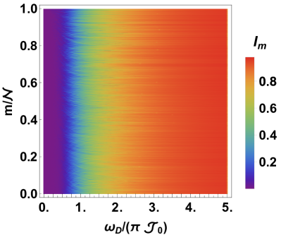
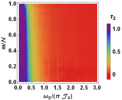
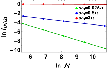
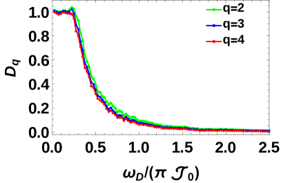
Figure 1: Top Left Panel: Plot of $I_{m}$ as a function of the normalized many-body eigenfunction index $m/\mathcal{N}$ and $\omega_{D}/(\pi\mathcal{J}_{0})$ showing the localized/delocalized nature of the Floquet eigenstates $|\psi_{m}\rangle$ for $L=14$. Top Right panel: Plot of $\tau_{2}$ as a function of $m/\mathcal{N}$ (after sorting in increasing order of $I_{m}$) and $\omega_{D}/(\pi\mathcal{J}_{0})$ showing the presence of delocalized states for $\omega_{D}/(\pi\mathcal{J}_{0})\leq 0.4$, multifractal states for $0.4\leq\omega_{D}/(\pi\mathcal{J}_{0})\leq 1.5$ and fully localized states for $\omega_{D}/(\pi\mathcal{J}_{0})>1.5$. The system sizes used for extracting $\tau_{2}$ are $L=10,\cdots,18$ in steps of $2$. Bottom Left panel: Plot for $\ln I_{m}$ vs $\ln L$ used for extracting $\tau_{2}$ for several representative frequencies for the state corresponding to $m/{\mathcal{N}}=0.5$. The behavior of perfectly delocalized (green dots at $\omega_{D}/(\pi\mathcal{J}_{0})=0.025$) and localized (red dots, $\omega_{D}/(\pi\mathcal{J}_{0})=3$) can be distinguished from that of a multifractal states (blue dots $\omega_{D}/(\pi\mathcal{J}_{0})=0.5$). Bottom Right Panel: Plot of $D_{q}$ as a function of $\omega_{D}/(\pi\mathcal{J}_{0})$ for $m/\mathcal{N}=0.5$. We have set $\mathcal{J}_{0}=1$, $V_{0}/\mathcal{J}_{0}=0.05$ , $V_{\rm int}/\mathcal{J}_{0}=0.025$ , scaled all energies and frequencies in units of $\mathcal{J}_{0}$ (with $\hbar$ set to unity). See text for details.

To analyze the nature of the Floquet eigenstates further, we first plot $\tau_{2}$ as a function of eigenvector index $m/{\mathcal{N}}$ and $\omega_{D}$ in the top right panel of Fig. 1. From this plot, we find the presence of ergodic and MBL states for low ($\hbar\omega_{D}/(\pi\mathcal{J}_{0})<0.4$) and high ($\hbar\omega_{D}/(\pi\mathcal{J}_{0})>1.5$) drive frequencies respectively. In between, one finds state with $0\leq\tau_{2}\leq 1$ signifying their non-ergodic and non-MBL nature. We note that for this plot we sort the eigenstates in increasing value of $I_{m}$. Thus we find that the states which had $0\leq I_{m}\leq 1$ also have $0\leq\tau_{2}\leq 1$; these states are natural candidate for multifractal Floquet eigenstates.

In what follows, we extract $\tau_{2}$ from the plot of $\ln I_{m}$ versus $\ln\mathcal{N}$ as shown in the bottom left panel of Fig. 1 for $m/{\mathcal{N}}=0.5$. For $\hbar\omega_{D}/(\pi\mathcal{J}_{0})=3$ the state is many-body localized and we have $\tau_{2}\sim 0$ as evident from the flat red line in the bottom left panel of Fig. 1. In contrast, at $\hbar\omega_{D}/(\pi\mathcal{J}_{0})=0.025$ we have $\tau_{2}=1$ (green line in bottom left panel of Fig. 1) signifying the ergodicity of the state. In between, at $\hbar\omega_{D}/(\pi\mathcal{J}_{0})=0.5$ , $\tau_{2}=0.4$ (blue line in bottom left panel of Fig. 1) indicating the presence of non-ergodic and non-MBL nature of the state.

The plot of the multifractal dimension $D_{q}$ is shown in bottom right panel of Fig. 1 for states corresponding to $m/{\mathcal{N}}=1/2$. For all points in these plots, $D_{q}$ is obtained from values of $\tau_{q}$ that are, in turn, extracted from the corresponding plots of $\ln I_{m}$ vs $\ln{\mathcal{N}}$. From the plot, we find that for $0.35\leq\hbar\omega_{D}/(\pi\mathcal{J}_{0})\leq 1.5$, $0\leq D_{q}\leq 1$; this indicates the presence of multifractal states in the spectrum. Other states with different $m/{\mathcal{N}}$ also show similar features. The behavior of $D_{q}$ shown in the bottom right panel of Fig. 1 indicates that the driven fermion chain exits the ergodic phase for $\hbar\omega_{D}/(\pi\mathcal{J}_{0})\simeq 0.4$. We note here that our numerical analysis shows that $D_{q}$ is almost independent of $q$ for $q\leq 4$; this indicates the possibility of fractal nature of these states. However, ascertaining this property would require computation of $\tau_{q}$ for all $q$ and we do not attempt this in the present work.

III.0.2 Shannon Entropy

To further establish the presence of the ergodic , multifractal and MBL phases as a function of frequency and to find out the nature of the transition between them, we study the Shannon entropy of the Floquet eigenstates. The Shannon entropy of the $m^{\rm th}$ Floquet eigenstate is given by

$$S_{m} = -\sum_{m}|c_{mn}|^{2}\ln|c_{mn}|^{2},\quad S=\frac{1}{\mathcal{N}}\sum_{m}S_{m}$$

where $S$ is the mean entropy. We note that for $\hbar\omega_{D}/(\pi\mathcal{J}_{0})\gg 1$, $c_{mn}\simeq\delta_{mn}$ leading to $S_{m}\simeq 0$; thus $S\to 0$ indicates many-body localized eigenfunctions. In contrast for $\hbar\omega_{D}/(\pi\mathcal{J}_{0})\ll 1$ when all Floquet eigenstates are ergodic, $c_{mn}\simeq 1/\sqrt{\mathcal{N}}$ for all $m$ leading to maximum entropy of $S=S_{\rm max}\simeq\ln\mathcal{N}$.

The left panel of Fig. 2 shows the plot of Shannon entropy normalized by $\ln\mathcal{N}$ as a function of $\hbar\omega_{D}/\mathcal{J}_{0}$ for different system sizes. Note that the plot for different system sizes cross each other around $\hbar\omega_{D}/\mathcal{J}_{0}\sim 0.43\pi$; this seems to indicate a transition between the ergodic and multifractal phases. To understand this feature further, we note that the functional form of $S$ can be written as alet

$$S = D_{1}\ln\mathcal{N}+b_{1}$$ (13)

where $D_{1}$ is the fractal dimension. It is known that $b_{1}$ is expected to change sign at the transition from ergodic to MBL phase. This results in a crossing point between the curves of $S$ of different sizes at the critical frequency alet . The plot of $b_{1}$ is shown in the right panel of Fig. 2. It indicates that delocalized phase $b_{1}<0$ whereas in the MBL phase $b_{1}>0$.

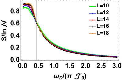
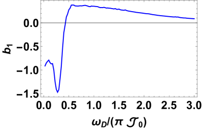
Figure 2: Left panel: Plot of $S/\ln\mathcal{N}$ as a function of $\omega_{D}/(\pi\mathcal{J}_{0})$ showing the presence of an ergodic to MBL transition at $\omega_{D}/(\pi\mathcal{J}_{0})\sim 0.44$. Right panel: Plot of $b_{1}$ as a function of $\omega_{D}/(\pi\mathcal{J}_{0})$ showing $b_{1}\leq 0$ in the ergodic phase whereas $b_{1}>0$ in the MBL phase . The plot at right panel shows that $b$ changes sign at $\omega_{D}/(\pi\mathcal{J}_{0})\sim 0.45$ suggesting a critical point. All other parameters are same as in Fig. 1. See text for details.

It is also instructive to study the fluctuations of entanglement entropy abanin , as they have been shown to provide a useful probe of the delocalization to MBL transition. The fluctuations of S is defined as,

$$\Delta S=\sqrt{\langle(S-\langle S\rangle)^{2}\rangle}$$ (14)

It is known that $\Delta S$ is small deep inside both the ergodic and MBL phases. In the ergodic phase, all Floquet eigenstates are highly entangled with $S=S_{\rm max}$. Thus the system exhibits small fluctuation around this value. In the MBL phase $S$ follows an area law and is hence small (compared to that in the ergodic phase where it follows volume law). In addition, since all states have low $S$, the fluctuations are small. In contrast, at the transition $S$ has a broad distribution leading to maximal value of $\Delta S$. Thus, the delocalization to MBL transition can be detected by the location of the peak in $\Delta S$.

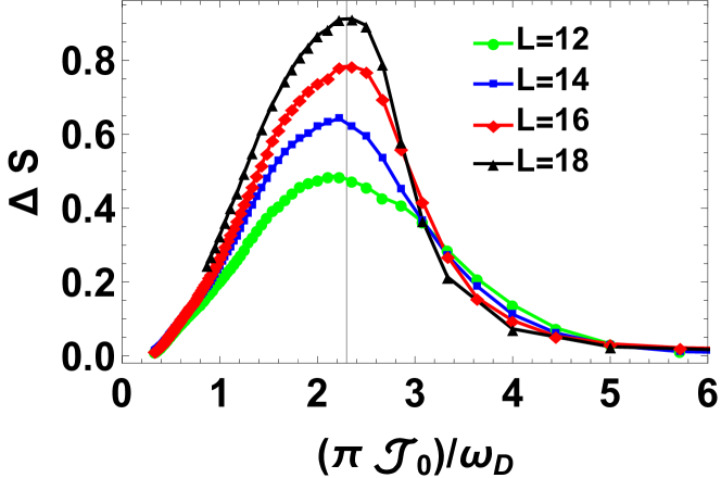
Figure 3: Plot of $\Delta S$ as a function of $(\pi\mathcal{J}_{0})/\omega_{D}$ showing that the transition from ergodic to the multifractal phase takes place at $\pi\mathcal{J}_{0}/\omega_{D}\sim 2.3$ or $\omega_{D}/\mathcal{J}_{0}\sim 0.434\pi$. All other parameters are same as in Fig. 1. See text for details.

Fig. 3 shows the plot of $\Delta S$ as a function of $\pi\mathcal{J}_{0}/\hbar\omega_{D}$ and confirms that such a peak appears at $(\pi\mathcal{J}_{0})/\hbar\omega_{D}\sim 2.3$. We note that the peak gets sharper with increasing system size with a slight shift towards higher $T$; this indicates that drive may possibly induce a transition between ergodic and non-ergodic(multifractal) states which shall survive for larger $L$. Combining the results of $D_{q}$ and $\Delta S$, we seem to find that within the finite system sizes that we can access, there is possible transition around $\hbar\omega_{D}/(\pi\mathcal{J}_{0})\simeq 1/2.3=0.434$. A more definite characterization of this possible transition would require access to larger system size which is outside the scope of the present work.

IV Quantum Dynamics

In this section we discuss dynamical signatures for the multifractal states in the region of intermediate frequencies. We divide this section to study three different timescales, namely, short, intermediate and long time steady state. We analyze the behavior of different correlation functions and entropies in different regimes. This analysis is expected to be useful from an experimental standpoint since achieving short-time coherent dynamics is easier in experiments. Thus the signatures of multifractal states visible in those time-scales, if any, is much easier to detect experimentally.

IV.1 Short-time Dynamics

In this section we shall study the evolution of a product initial state in the basis of $H$ in the short time regime, $n_{0}<10^{2}$ cycles. We look for possible signatures of multifractal eigenstates of $H_{F}$ in dynamics which are different from the dynamics induced by either ergodic and MBL eigenstates. Unless otherwise mentioned, all the quantities in this section are calculated by averaging over $N_{0}$ product initial states. We choose $N_{0}=500$ for sizes $L=12,14$, $N_{0}=100$ for sizes $L=16,18$, and $N_{0}=18[20]$ for $L=20[22]$. We have chosen $N_{0}$ such that the error bars are smaller than the size of points. To evolve the system, we have used standard Krylov subspace techniques. krylov .

We show several features which appear to be intermediate between ergodicity and MBL in the range of frequencies where multifractality appears in the Floquet spectrum. These features are present for all $L$ studied here and their presence is therefore expected to be independent of $L$ at least for the range of system sizes studied in this work. It is important to note that while the eigenstate properties are calculated for size $L=10-18$, the absence of significant deviation in results for all $L\leq 22$ seems to justify our claim of the presence of a non-ergodic multifractal regime for larger system sizes than what can be accessed by ED.

IV.1.1 Auto-correlation function

In order to distinguish between ergodic, multifractal and MBL phases, we resort to the measurement of temporal auto-correlation function. The auto-correlation function is a measure of retention of memory of system’s initial state rafael and is given by

$$\mathcal{A}_{j}(t)=\left(2\langle\hat{n}_{j}(t)\rangle-1\right)\left(2\langle\hat{n}_{j}(0)\rangle-1\right)$$ (15)

where $\mathcal{A}_{j}(t)$ is the temporal auto-correlator at site $j$ and time $t=n_{0}T$ and $\langle n_{j}(t)\rangle=\langle U^{\dagger}(n_{0}T,0)n_{j}(0)U(n_{0}T,0)\rangle$ is the expectation value of fermion number operator at site $j$ and time $t=n_{0}T$. We average this single site operator over different sites and over different random product initial states

$$\mathcal{A}(t)=\frac{1}{L}\left[\sum_{j=1}^{L}\mathcal{A}_{j}(t)\right]$$ (16)

where the square brackets indicate initial state averaging.

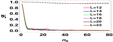
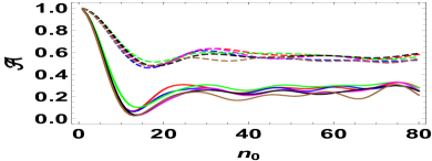
Figure 4: Plot of the temporal auto-correlation function as a function of number of cycles $n_{0}$. Left panel: Solid lines correspond to $\omega_{D}/(\pi\mathcal{J}_{0})=0.1$ (ergodic phase) while the dashed lines pertains to $\omega_{D}/(\pi\mathcal{J}_{0})=2.5$ (MBL phase). Right panel: Solid lines correspond to $\omega_{D}/(\pi\mathcal{J}_{0})=0.4$ near the transition from the ergodic to the multifractal regime while the dashed lines pertains to $\omega_{D}/(\pi\mathcal{J}_{0})=0.7$ (multifractal regime). All other parameters are same as in Fig. 1. See text for details.

We can distinguish between the three phases using the $\mathcal{A}$ versus $n_{0}$ plot as indicated in Fig. 4 where $n_{0}$ denotes the number of drive cycles. It is known that for short range systems that ${\mathcal{A}}$ displays exponential decay in the ergodic phase. This behavior is seen at low frequencies $\hbar\omega_{D}/(\pi\mathcal{J}_{0})=0.1$, as shown in the left panel of Fig. 4 (solid lines). The temporal auto-correlation function reduces to $1/L$ rapidly over a short interval of time. Due to the long range nature of the Floquet Hamiltonian, the decay deviates a bit from the usual exponential decay. In contrast, in the MBL phase at $\hbar\omega_{D}/(\pi{\mathcal{J}}_{0})>1.5$, the system is supposed to retain the memory of it’s initial state for a very long time. For short timescales ($n_{0}\leq 100$) studied in this section the auto-correlation does not decay significantly. This feature is seen at a high frequency of $\hbar\omega_{D}/(\pi\mathcal{J}_{0})=2.5$ in the left panel of Fig. 4 (dashed lines).

For the region of multifractal frequencies, it is not immediately clear how $\mathcal{A}$ should behave as the wavefunctions are extended but the system cannot be called ergodic. Our numerical result in the right panel of Fig. 4 shows that for $\hbar\omega_{D}/(\pi\mathcal{J}_{0})=0.4$ (solid line) and $0.7$ (dashed line), $\mathcal{A}$ shows a decay initially but then oscillates around a value which is intermediate to $1/L$ and $1$. The value of $\omega_{D}$ which controls the multifractal dimensions of the eigenstates of $H_{F}$ has effect on both the rate of the decay of ${\mathcal{A}}$ and its final value. This will be analyzed in details in subsequent sections. We note that for all $L$ considered,there is no significant finite size effect as can be seen from Fig. 5. Thus the behavior of ${\mathcal{A}}(n_{0})$ shown by Figs. 4 and 5 definitely points to the presence of a non-ergodic and non-MBL phase in the region of intermediate drive frequencies which supports multifractal eigenfunctions of $H_{F}$.

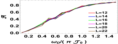
Figure 5: Plot of the temporal auto-correlation function as a function of $\omega_{D}/(\pi\mathcal{J}_{0})$ after a fixed number of cycles $n_{0}=80$ for different $L$. All other parameters are same as in Fig. 1. See text for details.

IV.1.2 Normalized Participation Ratio

One of the most common quantity to characterize delocalization-MBL transition is the measurement of the normalized participation ratio (NPR) which provides information about the volume of phase space explored by the system during dynamics rafael . The NPR is defined as

$$N_{p}^{(m)}(t) = \frac{1}{P_{m}(t)\mathcal{N}},\quad\zeta^{(m)}(t)=\ln N_{p}^{(m)}(t)$$ (17)

where $\mathcal{N}$ is the Hilbert space dimension, $t\in n_{0}T$, and $P_{m}(t)=\sum_{n}|d_{n}(t)|^{2m}$ is the dynamical IPR. In Eq. 17, $d_{n}(t)=\langle\chi_{n}|\psi^{\prime}\rangle$ where $|\psi^{\prime}\rangle=U(n_{0}T,0)|\psi_{\rm init}\rangle$ and $|\chi_{n}\rangle$ are the computational basis states. Here we choose several initial states $|\psi_{\rm init}\rangle$ and average $\zeta^{(m)}(t)$ over all such initial states. Also, for the rest of this section, we shall denote $\zeta(t)=[\zeta^{(2)}(t)]$ for clarity.

We note that $\zeta$(t) denotes the fraction of the configuration space that the system explores. In the delocalized phase we expect $\zeta(t)$ to be independent of $L$ and to reach the maximum value of zero when the system is uniformly ergodic. In the high frequency regime, when the system is in a MBL phase $\zeta(t)$ varies with $L$.

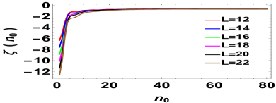
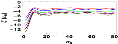
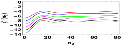
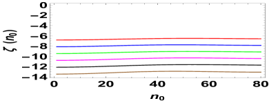
Figure 6: Plot of $\zeta$ as a function of $n_{0}$ for $\omega_{D}/(\pi\mathcal{J}_{0})=0.1$ corresponding to the ergodic regime (top left panel) and $\omega_{D}/(\pi\mathcal{J}_{0})=0.4$ near the transition from the ergodic to the multifractal regime (top right panel). The bottom left panel corresponds to $\omega_{D}/(\pi\mathcal{J}_{0})=0.7$ (multifractal regime) and the bottom right panel pertains to $\omega_{D}/(\pi\mathcal{J}_{0})=2.5$ (MBL phase). All other parameters are same as in Fig. 1. See text for details.

Fig. 6 shows the plot of $\zeta$ as a function of number of drive cycles $n_{0}$ for different frequencies. For $\hbar\omega_{D}/(\pi\mathcal{J}_{0})=0.1$, in the delocalized region, as shown in the top left panel of Fig. 6, $P_{m}\to 1/\mathcal{N}$ and hence $\zeta\to 0$. The plots for various system sizes therefore converges together to a $L$-independent near-zero value signifying ergodicity. In contrast, in the localized region $I_{m}\to 1$ and hence $\zeta\to-\ln\mathcal{N}$. Thus $\zeta$ varies with $L$ as shown in the bottom right panel of Fig. 6 for $\hbar\omega_{D}/(\pi\mathcal{J}_{0})=2.5$.

In the intermediate frequency regime, as shown for $\hbar\omega_{D}/(\pi\mathcal{J}_{0})=0.4(0.7)$ in top right(bottom left) panel of Fig. 6, we find $-\ln\mathcal{N}<\zeta<0$. This behavior, seen throughout the intermediate frequency range, shows that the phase space exploration originating from multifractal eigenstates of $H_{F}$ is faster than that due MBL eigenstates but slower than the ergodic ones. If the frequency is closer to the ergodic region where $\tau_{2}$ is closer to unity, $\zeta$ for different $L$ converge with increasing $\omega_{D}$. However, this behavior is different from the complete convergence found for ergodic Floquet eigenstates. As the drive frequency is increased, $\tau_{2}$ obtained from eigenstates of $H_{F}$ decreases. This leads to an increased separation (at the time scales studied here) of $\zeta$ for different $L$; moreover, the magnitude of change of $\zeta$ becomes smaller compared to the initial value. This intermediate behavior of $\zeta$ also points to the presence of non-ergodic and non-MBL states in agreement that seen from analysis of $\mathcal{A}$.

IV.1.3 Entanglement Entropy

In this section, we introduce half-chain von-Neumann entanglement entropy roop , denoted by $S_{vN}$ for the driven chain. $S_{vN}$ can be defined in terms of the reduced density matrix $\rho_{A}$ of the chain after $n_{0}$ drive cycles. This is computed by tracing out the density matrix $\rho=|\psi(n_{0}T)\rangle\langle\psi(n_{0}T)|$ (where $|\psi(n_{0}T)\rangle=U(n_{0}T,0)|\psi_{\rm init}\rangle$) over half the chain. In terms of this reduced density matrix $\rho_{A}$, one then obtains

$$S_{vN}(n_{0}T)=-{\rm Tr}[\rho_{A}(n_{0}T)\ln\rho_{A}(n_{0}T)].$$ (18)

For MBL states, $S_{vN}(n_{0}T)\sim\ln n_{0}$ if one starts from a homogeneous initial statenumberentrp ; in contrast $S_{vN}\sim n_{0}$ for ergodic states. For systems that support multifractal states there have some studies of how multifractal dimensions of states determine the entanglement entropymfracentr . For the present case, we note that the driven interacting fermion chain supports Floquet eigenstates of different multifractal dimensions controlled by $\omega_{D}$. Moreover, for a fixed $\omega_{D}$, it supports a spectrum of $\tau_{2}$ (Fig. 2). This suggests that the behavior of $S_{vN}$ for such eigenstates may be unconventional. However, one requires to probe into much larger time scales than that discussed in this subsection to probe the precise $n_{0}$ dependence of $S_{vN}$. This will be addressed in the next subsection where we discuss intermediate time behavior. Moreover, the measurement of $S_{vN}$ in experiments is a difficult task. In contrast, very recently, a different kind of entropy called number entropy has been shown to be experimentally measurable numberentr . We shall therefore study the short time behavior of the number entropy in the rest of this subsection.

In systems where the total particle number is conserved (which holds for the present case), the von-Neumann Entropy can be split into two partsnumberentr :

$$S_{vN}=S_{c}+S_{N}$$ (19)

where $S_{c}$ is the configuration entropy and $S_{N}$ is the number entropy. $S_{N}$ characterizes particle number fluctuation in the subsystem under consideration and is defined as,

$$S_{N}=-\sum_{n}p(n)\,\ln p(n)$$ (20)

where $p(n)$ is the probability of finding $n$ fermions within the subsystem (half chain for our case).

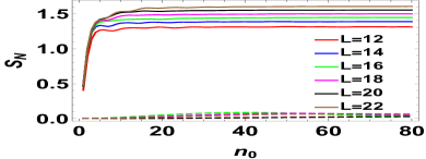
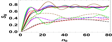
Figure 7: Plot of $S_{N}$ as a function of $n_{0}$. The solid lines in the left panel correspond to the ergodic phase ($\omega_{D}/(\pi\mathcal{J}_{0})=0.1$) while the dashed lines pertains to the MBL phase ($\omega_{D}/(\pi\mathcal{J}_{0})=2.5$). The solid lines in the right panel correspond to $\omega_{D}/(\pi\mathcal{J}_{0})=0.4$ (near the transition from the ergodic to the multifractal regime) and the dashed lines pertains to the multifractal phase ($\omega_{D}/(\pi\mathcal{J}_{0})=0.7$). All other parameters are same as in Fig. 1. See text for details.

It is expected that in ergodic phase, $S_{N}\sim\ln t$. Moreover, it has been numerically shown recently that in MBL phase (in contrast to the previously prediction of system size independent saturation), $S_{N}\sim\ln\ln t$. numberentrp . The study of the temporal dependence of $S_{N}$ to confirm such $\ln t$ (or $\ln\ln t$) behavior will be taken up in the next subsection. Here, we plot $S_{N}$ as a function of number of drive cycles $n_{0}$ for different representative drive frequencies at short-times and discuss whether there are any markers of the multifractal phase. The solid lines in the left panel of Fig. 7 shows the behavior of $S_{N}$ for $\hbar\omega_{D}/(\pi\mathcal{J}_{0})=0.1$ (ergodic regime); here $S_{N}$ seems to display a fast logarithmic growth before it saturates to an $L$ dependent value. The dashed lines in the left panel of Fig. 7 shows that for $\hbar\omega_{D}/(\pi{\mathcal{J}}_{0})=2.5$ (MBL phase) $S_{N}$ is almost a constant.

In the multifractal region , for $\hbar\omega_{D}/(\pi\mathcal{J}_{0})=0.4$ (solid line) and $0.7$ (dashed line) as shown in the right panel of Fig. 7, $S_{N}$ displays a sub-logarithmic growth followed by oscillations around a constant value. The amplitude of these oscillations increases with $L$ within the range of system sizes studied here. These features distinguish the multifractal phase from both the ergodic and the MBL phases and shows that $S_{N}$ carries signature of the multifractal phase realized at intermediate drive frequencies.

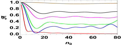
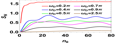
Figure 8: Left Panel: Plot of the temporal auto-correlation function for different frequencies within the range $0.1\leq\omega_{D}/(\pi\mathcal{J}_{0})\leq 2.5$ (shown by the legend on the right panel) as a function of number of drive cycles $n_{0}$. Right Panel: Similar plot of the number entropy $S_{N}$ as a function of $n_{0}$. All other parameters are same as in Fig. 1. See text for details.

We conclude this section by reinforcing how the short-time behavior of ${\mathcal{A}}$ and $S_{N}$ show differences in different regions of the drive frequency. To this end, in the left panel of Fig. 8, we plot $\mathcal{A}$ for $L=22$ and several representative $\omega_{D}$. The plot displays the nature of the decay of ${\mathcal{A}}$ in different drive frequency regimes. The slope of the decay gradually decreases with increasing frequency. The position of the first dip also slowly shifts towards higher $n_{0}$ with increasing $\omega_{D}$. Thus we find that for sufficiently large $n_{0}$, ${\mathcal{A}}$ settles to a frequency dependent value. The right panel shows a plot of $S_{N}$ for the same set of parameters and paints a similar qualitative picture. However, in contrast to the behavior of ${\mathcal{A}}$, here the change of growth is much sharper. This can be attributed to the fact that $S_{N}$ changes from logarithmic to sub-logarithmic growth with variation of $\omega_{D}$ and grows very slowly in the non-ergodic phase which is achieved at higher $\omega_{D}$. We note that growth rate is frequency independent and we shall discuss this feature in detail in the next section.

IV.2 Intermediate-time Dynamics

In this section, we discuss the dynamics of the driven interacting AA chain at intermediate stroboscopic time, i.e., for $n_{0}\sim 10^{3}$. This corresponds to a time scale which is an order of magnitude higher than that of the last section. We shall mainly concentrate on $S_{vN}$, which shows scaling laws in this time regime and also briefly discuss the behavior of $S_{N}$. Other quantities, such as ${\mathcal{A}}$, do not show any additional features and shall not be addressed here.

For this subsection, we start from the Neel or CDW initial state given by $|\psi_{0}\rangle=|1010...\rangle$. Such a choice is motivated by the results of Ref. inhomquench, , where it has been shown that the inhomogeneities in the initial state cause changes in the $\ln t$ growth of $S_{vN}$. In fermionic systems the most homogeneous state is expected to be the $|000..\rangle$ or $|111...\rangle$. However such initial states does not show any time evolution since the Floquet Hamiltonian conserves total particle number. Thus in the particle sector $N/2$, which constitutes the largest fraction of the Hilbert space, the most homogeneous product state is the CDW state.

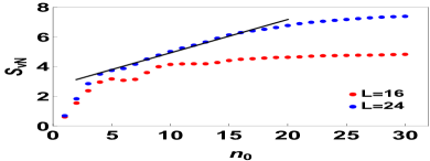
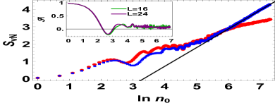
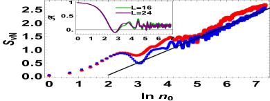
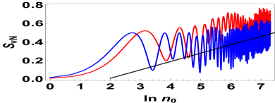
Figure 9: Top left panel: Plot of $S_{vN}$ as a function of $n_{0}$ for $\omega_{D}/(\pi\mathcal{J}_{0})=0.1$ (ergodic regime). Top right panel: Plot of $S_{vN}$ as a function of $\ln n_{0}$ for $\omega_{D}/(\pi\mathcal{J}_{0})=0.4$ near the transition from the ergodic to the multifractal regime. Bottom left panel: Same as top right panel but for $\omega_{D}/(\pi\mathcal{J}_{0})=0.55$ (multifractal regime). Bottom right panel: Same as top right panel but for $\omega_{D}/(\pi\mathcal{J}_{0})=1.0$ (MBL phase). All other parameters are same as in Fig. 1. See text for details.

Starting from $|\psi_{0}\rangle$, Fig. 9 shows the growth of $S_{vN}$ with $n_{0}$ for two different system sizes $L=16$ and $24$. As seen from the top left panel for $\hbar\omega_{D}/(\pi\mathcal{J}_{0})=0.1$, $S_{vN}$, in the ergodic phase, shows the expected initial linear growth followed by saturation to a $L$ dependent value. In contrast in the MBL phase, as shown in the bottom right panel for $\hbar\omega_{D}/(\pi\mathcal{J}_{0})=1.0$, we find a $\ln t$ growth of the entanglement, albeit with a very small slope. We note that in the high frequency regime each cycle represents a much smaller time step; in addition, the higher frequency also causes inherent dynamical localization dynloc3 which stretches the time the system requires to reach the steady state than that expected from an equilibrium MBL setup. This shows up as large oscillations in the plot. We also find that $L=16$ shows slightly faster growth in late times than $L=24$ for higher frequencies. This can be attributed to local effects of the Aubré Andre potential which become prominent due to localization(both dynamical and many-body) as frequency is increased.

For the multifractal region as seen from the top Right and the bottom left panels of Fig. 9($\hbar\omega_{D}/(\pi\mathcal{J}_{0})=0.45$ and $\hbar\omega_{D}/(\pi\mathcal{J}_{0})=0.55$ respectively), $S_{vN}$ is still found to follow a $\ln n_{0}$ growth. We note that the $\ln n_{0}$ growth of $S_{vN}$ at these frequencies shows up approximately at times after $\mathcal{A}$ has decayed towards its long-time value. In this regime, ${\mathcal{A}}$ oscillates around a non-zero frequency dependent steady-state value. This signifies presence of two different timescales in the problem and shows that the logarithmic growth of $S_{vN}$ need not be a feature just of MBL states for which the auto-correlation does not decay. Instead, it can also be feature of systems which are intermediate between ergodic and MBL. This points to a behavior $S_{vN}\sim a\ln n_{0}+b$ with $a$ and $b$ dependent on $\omega_{D}$.

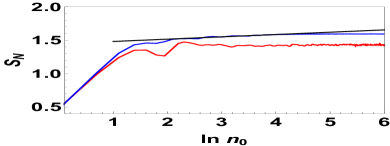
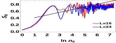
Figure 10: Left Panel: Plot of $S_{N}$ as a function of $n_{0}$ for $\hbar\omega_{D}/(\pi\mathcal{J}_{0})=0.1$ (ergodic regime) showing $\ln t$ behavior. Right Panel: Plot of $S_{N}$ as a function of $\ln n_{0}$ for $\omega_{D}/(\pi\mathcal{J}_{0})=0.55$ (multifractal regime) showing that the number entropy grows slower than $\ln t$ in this regime. All other parameters are same as in Fig. 1. See text for details.

Next, in Fig. 10, we address the behavior of $S_{N}$ as a function of $n_{0}$. The left panel of Fig. 10, for $\hbar\omega_{D}/(\pi\mathcal{J}_{0})=0.1$ (ergodic regime), we find a logarithmic increase in $S_{N}$ in the same timescales where $S_{vN}$ increases linearly with $n_{0}$(Fig. 9). We find that $S_{N}=1.46+0.03\ln n_{0}$ provides an accurate description of the behavior of $S_{N}$ in the ergodic regime. It is to be noted that the initial sharp rise in both $S_{vN}$ and $S_{N}$ is due to local effects and is not the long-time behavior we intend to study. In this long time regime, the growth is expected to be $\sim\ln\ln t$ as discussed in some recent MBL studies numberentrp2 . However, with the numerically accessible system sizes that we have, while we can confirm that the entanglement growth appears to be sub-logarithmic (the black line in the right panel of Fig. 10 shows a logarithmic fit), much larger system sizes and time scales are required to determine the exact form of the growth.

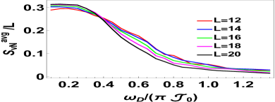
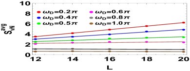
Figure 11: Left Panel: Plot of $S_{vN}/L$ averaged over ${\rm Int}[9000/T]-{\rm Int}[10000/T]$ cycles as a function of $\omega_{D}/(\pi\mathcal{J}_{0})$ for different $L$. The plots indicate crossing at $\omega_{D}/(\pi\mathcal{J}_{0})\sim 0.45$ for different $L$ which may signify a transition from the ergodic to multifractal regime. Right Panel: Plot of $S_{vN}/L$ averaged over ${\rm Int}[9000/T]-{\rm Int}[10000/T]$ cycles as a function of $L$ for representative frequencies. All other parameters are same as in Fig. 1. See text for details.

As seen from Fig. 9 the evolution of entropy can be fit to $S_{vN}(n_{0})\sim a\ln n_{0}+b$ where $a$ and $b$ are frequency dependent constants. We found that $a$ decreases as the frequency $\omega_{D}$ is increased for $0.45\leq\hbar\omega_{D}/(\pi\mathcal{J}_{0})\leq 0.8$ (in the multifractal regime). $a$ decreases sharply after the transition (around $\hbar\omega_{D}/(\pi{\mathcal{J}}_{0})=0.43$) from ergodic to the multifractal regime. For $\hbar\omega_{D}/(\pi{\mathcal{J}}_{0})>0.7$ $a$ approaches zero and becomes almost independent of $\omega_{D}$ signifying the onset of MBL region.

Finally, we study the plot of $S^{\rm av}$, which is average of $S_{vN}/L$ over ${\rm Int}[9000/T]\leq n_{0}\leq{\rm Int}[10000/T]$ cycles (where ${\rm Int}[x]$ denotes nearest integer to $x$), as a function of frequency. The corresponding plot is shown in the left panel of Fig. 11. Here, instead of looking at equal number cycles $n_{0}$, we study the behavior of the quantities averaged over equal span of stroboscopic time $n_{0}T$. This is done in the regime where $n_{0}T$ is large compared to other time scales in the model. As seen from the plot, we find a crossing around $\hbar\omega_{D}/(\pi\mathcal{J}_{0})\sim 0.4$. This is indicative of the transition from the ergodic to the multifractal regime as also seen earlier from the behavior of the Shannon entropy. The presence of such a crossing may be understood as follows. In this MBL regime, the system takes an exponentially long time to reach the steady state where the average $S$ ($S^{\rm av}$) obeys a volume law. Thus, for a fixed time, $S_{\rm av}$ decreases with system size since it stays closer to its steady state value for smaller $L$. In contrast, for the ergodic regime $S^{\rm av}$ reaches its steady state value at relatively short times. Hence $S^{\rm av}$ yields the steady state value which increases with $L$ in this regime. The fact that one finds a crossing between $S^{\rm av}$ for different $L$ is indicative of a length-scale independent transition point between the ergodic and the multifractal regimes. Finally, we note that $S^{\rm av}\sim a_{0}L$ in the steady state which indicates that it follows volume law in this regime. However, $a_{0}$ depends on the drive frequency and approaches zero as we enter the MBL regime. This is indicative of the large time scale required to approach the steady state as discussed earlier.

IV.3 Steady state

In this section we study the steady state properties of the system directly from the eigenfunctions of $H_{F}$. While in MBL regime it is extraordinarily difficult to experimentally reach this state due to the enormous timescales, it is still an important aspect to look at as features embedded in $H_{F}$ show up most prominently in this regime. In what follows, we shall study fermionic transport, auto-correlation function and the number entropy in the steady state.

IV.3.1 Transport

To study transport in the system, we start from a domain wall initial state defined in the fermion number basis by,

$$|\psi_{\rm init}\rangle=|n_{1}=1,...n_{L/2}=1,n_{L/2+1}=0,...n_{L}=0\rangle$$ (21)

where the system size $L$ was considered to be an even integer (chain with even number of sites) and $n_{j}=\langle\hat{n}_{j}\rangle$ denotes fermion occupation number on the $j^{\rm th}$ site. The wavefunction after $n$ drive cycles is then given by

$$|\psi^{\prime}\rangle = U(nT,0)|\psi_{\rm init}\rangle=\sum_{m}c_{m}^{\rm init}e^{-in\epsilon_{m}^{F}T/\hbar}|\psi_{m}\rangle$$ (22)

where $|\psi_{m}\rangle$ denotes Floquet eigenstates with $L/2$ fermions and $c_{m}^{\rm init}=\langle\psi_{m}|\psi_{\rm init}\rangle$. Using this state we study the following quantities in order to further establish the MBL transition.

$$N_{0j}(T) = \langle 2(\hat{n}_{j}-1/2)\rangle$$

$$\quad N_{\rm av}(T) = \frac{4}{L}\sum_{j=1..L}\langle\hat{(}\hat{n}_{j}-1/2)\rangle^{2}$$ (23)

where the average is taken with respect to the steady state reached under a Floquet drive starting from $|\psi_{\rm init}\rangle$. In terms of the Floquet eigenfunctions $|\psi_{m}\rangle$ and the overlap coefficients $c_{m}^{\rm init}$ (Eq. 22) these can be expressed as

$$N_{0j}(T) = \sum_{m}|c_{m}^{\rm init}|^{2}\langle\psi_{m}|2(\hat{n}_{j}-1/2)|\psi_{m}\rangle$$ (24)

$$N_{\rm av}(T) = \frac{4}{L}\sum_{j=1..L}(\sum_{m}|c_{m}^{\rm init}|^{2}\langle\psi_{m}|\hat{(}\hat{n}_{j}-1/2)|\psi_{m}\rangle)^{2}$$

We note that for the initial state $|\langle\psi_{\rm init}|\hat{2}(\hat{n}_{j}-1/2)|\psi_{\rm init}\rangle|^{2}=-1$ for j $<$ L/2 and $|\langle\psi_{\rm init}|\hat{2}(\hat{n}_{j}-1/2)|\psi_{\rm init}\rangle|^{2}=1$ for j $>$ L/2, while for free fermions, the ground state with $\mathcal{J}_{0}\gg V_{0}$, $\langle 2(\hat{n}_{j}-1/2)\rangle=0$. Thus $N_{\rm av}(T)$ provides a measure of degree of delocalization of the driven chain. A similar reasoning shows that $N_{0j}\to 0$ for all sites in the delocalized regime and $N_{0j}=1[-1]$ for $j<[>]L/2$ in the localized regime; in contrast, in the presence of a mobility edge, $N_{0j}$ takes values between $0$ and $1$ at different sites.

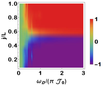
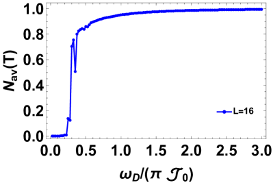
Figure 12: Left: Plot of $N_{0}$ as a function of $j/L$ and $\omega_{D}/(\pi\mathcal{J}_{0})$ showing fermion density profile at all sites of the chain in the steady state as a function of $\omega_{D}/(\pi\mathcal{J}_{0})$. Right: Plot of $N_{\rm av}(T)$ as a function of $\omega_{D}/(\pi\mathcal{J}_{0})$ in the steady state showing $0\leq N_{\rm av}(T)\leq 1$ for $0.3\leq\omega_{D}/(\pi\mathcal{J}_{0})\leq 1.5$. All other parameters are same as in Fig. 1. See text for details.

A plot of $N_{0}$ as a function of $j/L$ and $\omega_{D}$, shown in the left panel Fig. 12, indicates that the transition from the ergodic to the multifractal and MBL regions leaves it signature in fermion transport. We find that the steady state value of $N_{0}$ in the MBL (high frequency) regime is $\sim\pm 1$ for the left and right halves of the chain respectively. This indicates that the steady state is close to the initial state as expected in the MBL regime. In contrast, $N_{0}=0$ for all $j/L$ in the ergodic (low frequency) regime which indicates that the system has reached the infinite temperature steady state as expected for a driven ergodic many-body system. In between, the system displays a range values of $N_{0}$ for different $j$ which indicates the intermediate behavior in the multifractal regime. This is also reflected in the plot of $N_{\rm av}$ which shows a kink in the multifractal regime and indicates a transition between the localized and delocalized regimes. We note here that the steady state localization here happens due to both MBL nature of the Floquet eigenstates and dynamical localization due to the drive; thus fermion transport may not solely reflect MBL properties in the high frequency regime.

IV.3.2 Auto-correlation function

We define the steady state auto correlation function at site $j$ as,

$$\mathcal{A}_{s}^{j}=(2n_{j}^{s}-1)(2n_{j}^{0}-1)$$ (25)

where ,

$$n_{j}^{s}=\sum_{m}|c_{m}^{\rm init}|^{2}\langle\psi_{m}|\hat{n}_{j}|\psi_{m}\rangle$$

the steady state value of $\langle\hat{n}_{j}\rangle$ and $n_{j}^{0}=\langle\psi_{\rm init}|\hat{n}_{j}|\psi_{\rm init}\rangle$ is the initial value. We average this single site operator over different sites to compute $\mathcal{A}_{s}^{\rm av}=\frac{1}{L}\sum_{j}\mathcal{A}_{s}^{j}$.

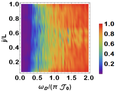
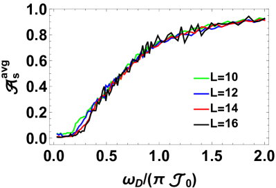
Figure 13: Left: Plot of $\mathcal{A}_{s}$ as a function of $j/L$ and $\omega_{D}/(\pi\mathcal{J}_{0})$ showing the auto-correlation at all sites of the chain in the steady state as a function of $\omega_{D}/(\pi\mathcal{J}_{0})$. Right: Plot of $\mathcal{A}_{s}^{\rm avg}$ as a function of $\omega_{D}/(\pi\mathcal{J}_{0})$. All other parameters are same as in Fig. 1. See text for details.

The left panel of Fig. 13 shows the plot of steady state value of the auto-correlation function as a function of $j$ and $\omega_{D}$. This value is computed by averaging over $N_{0}=50$ product initial states in the basis of $H$ for $L=10-14$ and $N_{0}=10$ such states for $L=16$. Below $\hbar\omega_{D}/(\pi\mathcal{J}_{0})\sim 0.25$, the value of autocorrelator remains zero indicating $n_{j}^{s}=1/2$ for all $j$ in the steady state. In contrast at high drive frequencies, one expects $n_{j}^{s}\simeq n_{j}^{0}$ leading to ${\mathcal{A}}^{\rm av}\simeq 1$. In between $0.25<\hbar\omega_{D}/(\pi\mathcal{J}_{0})<1$, the behavior is intermediate to that of delocalized or MBL phase. Thus $0<{\mathcal{A}}_{s}<1$ indicates that the system is in a multifractal phase. As the frequency is increased beyond that, $\mathcal{A}_{s}\to 1$ indicating the onset of localization. As before, we point out that this localization receives contribution from both the MBL nature of the Floquet eigenstates and the dynamical localization due to the drive.

IV.3.3 Number entropy

In this subsection we shall show the steady state behavior of $S_{N}$ denoted by $S_{N}^{s}$. We divide the system into two subsystems $A$ and $B$ and we integrate over subsystem $B$. To compute the number entropy, we first denote the states in the fermion number basis as $|\chi_{k}\rangle$. Since these are eigenstates of the number operator, for each of them, one can compute the total number of fermions $n$ in subsystem A: $n_{Ak}=\sum_{j\in A}\langle\chi_{k}|\hat{n}_{j}|\chi_{k}\rangle$. Using the notation of Eq. 22, we can write in the steady state

$$|d_{k}^{s}|^{2} = |\langle\chi_{k}|\psi_{m}\rangle|^{2}=\sum_{m}|c_{m}^{\rm init}|^{2}|\langle\chi_{k}|\psi_{m}\rangle|^{2}$$ (26)

Using Eq. 26, we can then obtain

$$p_{s}(n) = \sum_{k=k^{\prime}}|d^{s}_{k}|^{2}$$ (27)

$$S_{N}^{s} = -\sum_{n}p_{s}(n)\ln p_{s}(n),\,\,\langle S_{N}^{s}\rangle=\frac{1}{N}\sum_{i}^{N}S_{N}^{s}(i)$$

where $k^{\prime}$ denotes all states with $n_{Ak}=n$. Here $\langle S_{N}^{s}\rangle$ denotes averaged number entropy where the average is taken over $N$ product states. For an initial Neel state, we denote the entropy by $\mathcal{S}_{N}^{s}$ since no averaging is involved.

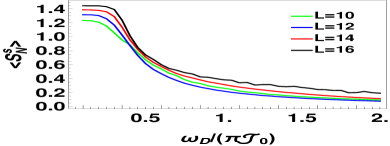
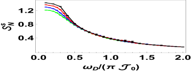
Figure 14: Left: Plot of $\langle S_{N}^{s}\rangle$ as a function of $\omega_{D}/(\pi\mathcal{J}_{0})$ showing the decrease in number entropy with increasing frequency For sizes $L=10,12,14$ we have averaged over all possible product initial states, for $L=16$ we have averaged over several random product states such that the error bar is smaller than line width. Right: Plot of $S_{N}$ vs $\omega_{D}/(\pi\mathcal{J}_{0})$ for $|\psi_{\rm init}\rangle$ being the Neel state. All other parameters are same as in Fig. 1. See text for details.

Fig. 14 shows the steady state behavior of $S_{N}$ for different drive frequencies. The left panel shows the average behavior when we take $\ell$ product states: $|\psi_{\rm init}\rangle=|\chi_{\ell}\rangle$. We compute $\langle S_{N}^{s}\rangle$ by averaging over these states. In the low frequency regime where ergodicity is expected, $\langle S_{N}^{s}\rangle$ is large and monotonically increases with $L$. However with increasing frequency as the system becomes non-ergodic, it decreases and there is no clear monotonicity with $L$. This is similar to the behavior seen in Ref. numberentrp2, . A similar behavior is also seen on the right panel where $|\psi_{\rm init}\rangle$ is taken to be the Neel state. For these plots, we have chosen the AA potential to be $V_{j}=V_{0}\cos(2\pi\eta j+\phi)$ and have averaged over $\phi$ to smoothen out possible local fluctuations. These local fluctuations tend to arise in $S_{N}$ at high frequencies as the steady state values heavily depend on the local potentials near the half-chain cut. To prevent this from affecting our overall result we perform the averaging in this scenario. From the plot, we find that at large drive frequencies (i.e., in the localized regime), the steady state curves for different $L$ almost overlap. In contrast, in the ergodic regime there is a clear increase of $S_{N}$ with system size. The plot confirms that the system is localized at high frequencies but not at intermediate frequencies.

V Floquet Perturbation Theory

In this section, we aim to obtain a semi-analytic, albeit perturbative, understanding of several features of the driven interacting AA model found via exact numerics using a Floquet perturbation theory which is known to provide accurate results at intermediate frequencies provided that the term in $H(t)$ with largest amplitude is treated exactlydynloc3 ; rev9 . In the present case, since ${\mathcal{J}}_{0}\gg V_{0},V_{\rm int}$, one needs to treat the drive term exactly. Thus one obtains

$$U_{0}(t,0) = e^{i{\mathcal{J}}_{0}t\sum_{k}\epsilon_{k}\hat{n}_{k},/\hbar}\quad t\leq T/2$$ (28)

$$= e^{i{\mathcal{J}}_{0}(T-t)\sum_{k}\epsilon_{k}\hat{n}_{k}/\hbar}\quad t\geq T/2$$

where $U_{0}$ is the exact evolution operator corresponding to $H=H_{0}={\mathcal{J}}_{0}\sum_{k}\epsilon_{k}\hat{n}_{k}$ and $\epsilon_{k}=-2\cos k$ for the fermion chain with nearest-neighbor hopping. From Eq. 28, we find that $U_{0}(T,0)=I$ indicating $H_{F}^{(0)}=0$.

Next, we compute the first order Floquet Hamiltonian $H_{F}^{(1)}$. To this end, we note that within first order perturbation theory, the correction to the evolution operator is given by rev9

$$U_{1}(T,0) = \frac{-i}{\hbar}\int_{0}^{T}dtU_{0}^{\dagger}(t,0)(H_{1}+H_{A})U_{0}(t,0)$$

$$H_{F}^{(1)} = \frac{i}{T}U_{1}(T,0)$$ (29)

The computation of $H_{F}^{(1)}$ can be done in a straightforward manner following the method discussed in Refs. dynloc3, ; rev9, . The matrix elements of $H_{F}^{(1)}$ between Fock states in momentum space, denoted by $|n_{k}\rangle=|n^{(1)}_{k_{1}}.....n^{(N)}_{k_{N}}\rangle$, is given by

$$\langle n_{i}|H_{F}^{(1)}|n_{f}\rangle = V_{0}\sum_{q,k_{1}}\frac{2\hbar(1-e^{iT\mathcal{J}_{0}\alpha_{1}(k_{1},q)/\hbar})}{T\mathcal{J}_{0}\alpha_{1}(k_{1},q)}f(q)\delta_{n^{i}_{k_{1}},n^{f}_{k_{1}+q}-1}$$

$$+V_{\rm int}\sum_{k_{1},k_{2},q}\frac{2\hbar(1-e^{iT\mathcal{J}_{0}\alpha_{2}(k_{1},k_{2},q)/\hbar})}{T\mathcal{J}_{0}\alpha_{2}(k_{1},k_{2},q)}e^{-iq}\delta_{n_{i}^{k_{1}},n_{f}^{k_{1}}-1}\delta_{n_{i}^{k_{2}},n_{f}^{k_{2}}-1}\delta_{n_{f}^{k_{2}-q},n_{i}^{k_{2}-q}+1}\delta_{n_{f}^{k_{1}+q},n_{i}^{k_{1}+q}+1}$$

$$\alpha_{1}(k_{1},q) = \cos k_{1}-\cos(k_{1}+q),\quad\alpha_{2}(k_{1},k_{2},q)=\cos k_{1}+\cos k_{2}-\cos(k_{1}+q)-\cos(k_{2}-q)$$ (30)

where $f(q)=\sum_{j}\exp[-ijq]\cos(2\pi\eta j)$. We note that for $T\to 0$, the Floquet Hamiltonian reduces to that obtained from the first order Magnus expansion $H_{F}^{(1)}(T\to 0)\simeq H_{F}^{\rm magnus}=H_{A}+H_{1}$. However at intermediate frequencies, the frequency dependence of $H_{F}^{(1)}$ is much more complicated. Moreover, a similar calculation shows that $U_{2}(T,0)=U_{1}(T,0)^{2}/2$; thus $H_{F}^{(2)}=0$ and $H_{F}^{(1)}$ represents the sole contribution to $H_{F}$ to ${\rm O}(T^{2})$. These features allow one to expect that it shall provide at least qualitatively accurate description of the dynamics of the system at intermediate drive frequencies.

Next, we use Eq. 30 to numerically compute matrix elements of $H_{F}^{(1)}$ between Fock states in the position basis. A numerical diagonalization of the matrix thus obtained yields the eigenvalues and eigenvectors (in the real space Fock basis) for comparison with our exact results.

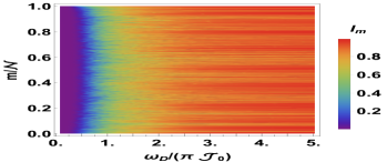
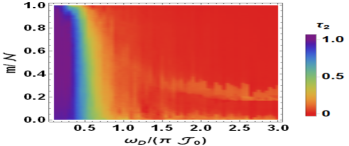
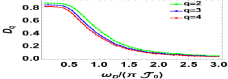
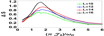
Figure 15: Top Left: Plot of $I_{m}$ as a function of the normalized many-body eigenfunction index $m/\mathcal{N}$ and $\omega_{D}/(\pi\mathcal{J}_{0})$ showing the localized/delocalized nature of the Floquet eigenstates $|\psi_{m}\rangle$ for $L=14$. Top Right: Plot of $\tau_{2}$ as a function of $m/\mathcal{N}$ (after sorting in increasing order of $I_{m}$) and $\omega_{D}/(\pi\mathcal{J}_{0})$ showing the presence of delocalized states for $\omega_{D}/(\pi\mathcal{J}_{0})\leq 0.45$, multifractal states for $0.45\leq\omega_{D}/(\pi\mathcal{J}_{0})\leq 1.5$ and localized states for $\omega_{D}/(\pi\mathcal{J}_{0})>1.5$ . The system sizes used for extracting $\tau_{2}$ are $L=10,\cdots,16$ in steps of $2$. Bottom Left : Plot of $D_{q}$ as a function of $\omega_{D}/(\pi\mathcal{J}_{0})$ for $m/\mathcal{N}=0.5$. Bottom Right: Plot of $\Delta S$ as a function of $(\pi\mathcal{J}_{0})/\omega_{D}$. All these plots has been done using FPT and parameters are same as in Fig. 1. See text for details.

The results obtained from the above-mentioned procedure is depicted in Fig. 15. From Fig. 15 we find that the results obtained from FPT agrees with those from exact numerics discussed in Sec. III. The top left panel of Fig. 15 shows the plot of $I_{m}$, obtained from eigenvectors of $H_{F}^{(1)}$ using Eq. 10, as a function of $\omega_{D}$. The top right panel shows the corresponding plot for $\tau_{2}$. We find that both the plots show similar multifractal behavior as seen in Figs. 1 and 2 within similar range of $\omega_{D}/(\pi\mathcal{J}_{0})$. In particular, we find that the eigenvectors of $H_{F}^{(1)}$ exhibits delocalized eigenstates for $\omega_{D}/(\pi\mathcal{J}_{0})\leq 0.45$, multifractal eigenstates states for $0.45\leq\omega_{D}/(\pi\mathcal{J}_{0})\leq 1.5$ and localized eigenstates for $\omega_{D}/(\pi\mathcal{J}_{0})>1.5$. The plot of $D_{q}$ as a function of $\omega_{D}$, shown in the bottom left panel of Fig. 15, also shows qualitatively similar behavior to that obtained from ED shown in bottom right panel of Fig. 1; however, we note that the change in $D_{q}$ signifying the transition to multifractal phase is seen around $\hbar\omega_{D}/(\pi{\mathcal{J}}_{0})\simeq 0.6$. Thus the position of the transition is not accurately captured by $H_{F}^{(1)}$. Nevertheless, $H_{F}^{(1)}$ does predict the transition to the multifractal phase as seen in the bottom right panel of Fig. 15, where a plot of $\Delta S$ as a function of $\omega_{D}$ shows a distinct peak. The peak becomes sharper with increasing $L$ which is consistent with the result obtained from ED. Thus we conclude that $H_{F}^{(1)}$, computed using FPT, constitutes a semi-analytic Floquet Hamiltonian which shows a transition from ergodic to multifractal regime at intermediate frequencies.

VI Discussion

In this work, we have studied a driven fermionic chain with an AA potential and nearest neighbor density-density interaction between the fermions. Our analysis constitutes a detailed study, both numerical and semi-analytic, of the Floquet Hamiltonian of such a system as a function of drive frequency in the limit of large drive amplitude.

We have shown that such a driven system supports multifractal many-body Floquet eigenstates for a range of drive frequencies in the intermediate drive frequency regime. We find that the eigenstates are ergodic in the low frequency and many-body localized in the high drive frequency regime. In between, for system sizes accessible in our numerics, results indicate a possible transition from ergodic to multifractal phase at $\omega_{D}=\omega_{c}\simeq 0.43{\mathcal{J}}/\hbar$. Upon further increasing the drive frequency, the eigenstates become many-body localized via a smooth crossover. The presence of the transition from ergodic to the multifractal phase seems likely due to two reasons. First, the plot of entropy fluctuation $\Delta S$ as a function of $T$ shows a peak at the transition which gets sharper with increasing system size. Second, $b_{1}$ (Eq. 13) changes sign at this point which is indicative of a transition from the ergodic phase. However, we need that one needs finite size numerics with larger system size to settle this issue; this has not been attempted in this work.

Our analysis indicates that several dynamic quantities that we study can distinguish between the multifractal ergodic and MBL phases. These include the fermion auto-correlation function and the short time behavior of the normalized participation ratio. The former quantity decays sharply to zero in the ergodic phase due to spreading of the system in the Hilbert space. In the MBL phase, it remains close to its initial value since the system retains its initial memory. In the multifractal phase, we find an initial sharp decay of the auto-correlation function, followed by oscillation around a steady state value which is intermediate between its ergodic (zero) and the MBL (unity) counterparts. The latter quantity shows system-size independent behavior as a function of number of drive cycles in the ergodic phase and displays a clear $L$ dependence in the MBL phase. In contrast, it shows intermediate behavior with oscillations as a function of $n_{0}$ in the multifractal phase. We note that in contrast, the entanglement entropy and the number entropy do not distinguish between the multifractal and the MBL eigenstates.

We have also studied steady state properties of the driven system, starting from a domain wall initial state, by computing transport properties, auto-correlation function and the number entropy. We find all of these quantities reflect a change from localized to delocalized regime as a function of drive frequency. However, the localization seen in transport also receives contribution from dynamical localization at high drive frequencies dynloc3 . We also find that near the transition frequency, the distribution of the number density of fermions in the steady state acquires a large width; this suggests a possible signature of the multifractal regime in fermion transport. A similar feature is seen in the steady state value of auto-correlation function which satisfies $0<{\mathcal{A}}_{s}<1$ in the multifractal phase; this is in sharp contrast to its values zero and unity in the ergodic and MBL phases respectively. The plot of steady state number entropy also show a sharp drop at the transition which becomes sharper with increasing $L$.

We have also obtained similar qualitative features for the driven fermionic chain from a semi-analytic, albeit perturbative, Floquet Hamiltonian computed using FPT. Remarkably, this perturbative Floquet Hamiltonian reproduces multifractality of the Floquet eigenstates and also points towards a transition from the ergodic to the multifractal regime. Our results thus constitutes an analytic Floquet Hamiltonian which support ergodic, multifractal and MBL eigenstates depending on the drive frequency.

Our results could be relevant for ultracold interacting fermions in the presence of an 1D optical lattice rev8 . The realization of the AA potential can be done using techniques discussed in Refs. exp2, and exp22, . The drive can be implemented by appropriate tuning of the strength of the laser used to create the optical lattice. We suggest measurement of density-density auto-correlation of the fermions. Our results suggest that the short time behavior of this auto-correlation function would be sufficient to distinguish between the ergodic, MBL and the multifractal phases. In particular, in the intermediate drive frequency regime, we expect the auto-correlation function to exhibit a sharp drop followed by oscillations around a finite non-zero value.

The fate of the multifractal phase that we obtain in the thermodynamic limit remains an open question. The phase remains stable within the system sizes that we could access within ED; however, it is possible that it might either shrink for large $L$ leading to a direct ergodic-MBL quantum phase transition. An investigation of the stability of the multifractal phase in the thermodynamic limit is beyond the scope of the present paper. We note however, that the finite-sized chains that we study in this paper may possibly be experimentally realized using ultracold atoms in optical lattices.

- (1)
- (2) P. W. Anderson, Phys. Rev. 109, 1492 (1958); E. Abrahams, P. W. Anderson, D. C. Licciardello, and T. V. Ramakrishnan, Phys. Rev. Lett. 42, 673 (1979).
- (3) P. A. Lee and T. V. Ramakrishnan, Rev. Mod. Phys. 57, 287 (1985).
- (4) S. Aubry and G. Andre, Ann. Isr. Phys. Soc. 3, 133 (1980).
- (5) M. Ya. Azbel, Sov. Phys. JETP 17, 665 (1963).
- (6) M. Ya. Abzel, ibid. 19, 634 (1964).
- (7) M. Ya Abzel, Phys. Rev. Lett. 43, 1954 (1979).
- (8) J. Biddle, B. Wang, J. D. J. Priour, and S. D. Sarma, Phys. Rev. A, 80, 021603(R) (2009).
- (9) D. J. Boers, B. Goedeke, D. Hinrichs, and M. Holthaus, Phys. Rev. A, 75, 063404 (2007).
- (10) R. Riklund, Y. Liu, G. Wahlstrom, and Z. Zhao-bo, J. Phys. C: Solid State Phys., 19, L705 (1986).
- (11) F. A. B. F. de Moura, A. V. Malyshev, M. L. Lyra, V. A. Malyshev, and F. Dominguez-Adame, Phys. Rev. B, 71, 174203 (2005).
- (12) A. V. Malyshev, V. A. Malyshev, and F. Dominguez- Adame, Phys. Rev. B, 70, 172202 (2004).
- (13) S.-J. Xiong and G.-P. Zhang, Phys. Rev. B, 68, 174201 (2003).
- (14) A. Rodriguez, V. A. Malyshev, G. Sierra, M. A. Martin-Delgado, J. Rodríguez-Laguna, and F. Domínguez-Adame, Phys. Rev. Lett. 90, 027404 (2003).
- (15) S. Das Sarma, A. Kobayashi, and R. E. Prange, Phys. Rev. Lett. 56, 1280 (1986).
- (16) J. Biddle and S. Das Sarma, Phys. Rev. Lett. 104, 070601 (2010).
- (17) X. Deng, S. Ray, S. Sinha, G. V. Shlyapnikov, and L. Santos, Phys. Rev. Lett. 123, 025301 (2019).
- (18) D-L Deng, S. Ganeshan, X. Li, R. Modak, S. Mukerjee, and J. H. Pixley, Ann. Phys. 529, 1600399 (2017).
- (19) Z. Xu, H. Huangfu, Y. Zhang and S.Chen, New J. Phys. 22 , 013036 (2020).
- (20) A. Jagannathan, arXiv:2012.14744 (unpublished).
- (21) G. Roati, C. D. Errico, L. Fallani, M. Fattori, C. Fort, M. Zaccanti, G. Modugno, M. Modugno, and M. Inguscio, Nature (London) 453, 895 (2008).
- (22) B. Deissler, M. Zaccanti, G. Roati, C. D. Errico, M. Fattori, M. Modugno, G. Modugno, and M. Inguscio, Nat. Phys. 6, 87 (2010).
- (23) M. Schreiber, S. S. Hodgman, P. Bordia, H. P. L¨schen, M. H. Fischer, R. Vosk, E. Altman, U. Schneider, and I. Bloch, Science 349, 842 (2015).
- (24) H. P. Lauschen, P. Bordia, S. Scherg, F. Alet, E. Altman, U. Schneider, and I. Bloch, Phys. Rev. Lett. 119, 260401 (2017).
- (25) J. Dziarmaga, Adv. Phys. 59, 1063 (2010).
- (26) A. Polkovnikov, K. Sengupta, A. Silva, and M. Vengalattore, Rev. Mod. Phys. 83, 863 (2011).
- (27) A. Dutta, G. Aeppli, B. K. Chakrabarti, U. Divakaran, T. F. Rosenbaum, and D. Sen, Quantum phase transitions in transverse field spin models: from statistical physics to quantum information (Cambridge University Press, Cambridge, 2015).
- (28) S. Mondal, D. Sen, and K. Sengupta, Quantum Quenching, Annealing and Computation, edited by Das, A., Chandra, A. & Chakrabarti, B. K. Lecture Notes in Physics, Vol. 802 (Springer, Berlin, Heidelberg, 2010), Chap. 2, p. 21; C. De Grandi and A. Polkovnikov, ibid, Chap 6, p. 75.
- (29) M. Bukov, L. D’Alessio and A. Polkovnikov, Adv. Phys. 64, 139 (2015).
- (30) L. D’Alessio and A. Polkovnikov, Ann. Phys. 333, 19 (2013).
- (31) L. D’Alessio, Y. Kafri, A. Polokovnikov, and M. Rigol, Adv. Phys. 65, 239 (2016).
- (32) I. Bloch, J. Dalibard, and W. Zwerger, Rev. Mod. Phys. 80, 885 (2008); L. Taurell and L. Sanchez-Palencia, C. R. Physique 19, 365 (2018).
- (33) A. Sen, D. Sen, and K. Sengupta, arXiv:2102.00793 (unpublished).
- (34) T. Nag, S. Roy, A. Dutta, and D. Sen, Phys. Rev. B 89, 165425 (2014).
- (35) T. Nag, D. Sen, and A. Dutta, Phys. Rev. A 91, 063607 (2015).
- (36) A. Agarwala, U. Bhattacharya, A. Dutta, and D. Sen, Phys. Rev. B 93, 174301 (2016).
- (37) A. Agarwala and D. Sen, Phys. Rev. B 95, 014305 (2017).
- (38) D. J. Luitz, Y. Bar Lev, and A. Lazarides, SciPost Phys. 3, 029 (2017).
- (39) D. J. Luitz, A. Lazarides, and Y. Bar Lev, Phys. Rev. B 97, 020303 (2018)
- (40) R. Ghosh, B. Mukherjee, and K. Sengupta, Phys. Rev. B 102, 235114(2020).
- (41) A. Das, Phys. Rev. B 82, 172402 (2010).
- (42) S Bhattacharyya, A Das, and S Dasgupta, Phys. Rev. B 86 054410 (2010).
- (43) S. Hegde, H. Katiyar, T. S. Mahesh, and A. Das, Phys. Rev. B 90, 174407 (2014)
- (44) S. Mondal, D. Pekker, and K. Sengupta, Europhys. Lett. 100, 60007 (2012).
- (45) U. Divakaran and K. Sengupta, Phys. Rev. B 90, 184303 (2014); B. Mukherjee.
- (46) B. Mukherjee, A. Sen, D. Sen, and K. Sengupta, Phys. Rev B 102, 075123 (2020).
- (47) J. M. Deutsch, Phys. Rev. A 43, 2046 (1991).
- (48) M. Srednicki, Phys. Rev. E 50, 888 (1994); ibid., J. Phys. A 32,1163 (1999).
- (49) M. Rigol, V. Dunjko, and M. Olshanii, Nature (London) 452, 854 (2008).
- (50) L. D’Alessio and M. Rigol, M. Phys. Rev. X 4, 041048 (2014).
- (51) C. J. Turner, A. A. Michailidis, D. A. Abanin, M. Serbyn, and Z. Papic, Z. Nat. Phys. 14, 745 (2018).
- (52) C. J. Turner, A. A. Michailidis, D. A. Abanin, M. Serbyn, and Z. Papic, Phys. Rev. B 98,155134 (2018).
- (53) K. Bull, I. Martin, and Z. Papic, Phys. Rev. Lett. 123, 030601 (2019).
- (54) V. Khemani, C. R. Lauman, and A. Chandran, Phys. Rev. B 99, 161101 (2019).
- (55) S. Maudgalya, N. Regnault, and B. A. Bernevig, Phys. Rev. B 98, 235156 (2018).
- (56) T. Iadecola, M. Schecter, and S. Xu, arXiv:1903.10517 (unpublished).
- (57) N. Shiraishi, arXiv:1904.05182 (unpublished).
- (58) M. Schecter, and T. Iadecola, arXiv:1906.10131 (unpublished).
- (59) P. A. McClarty, M. Haque, A. Sen, and J. Richter, Phys. Rev. B 102, 224303 (2020).
- (60) D. Banerjee and A. Sen, Phys. Rev. Lett. 126, 220601 (2021).
- (61) B. Mukherjee, S. Nandy, A. Sen, D. Sen and K. Sengupta, Phys. Rev B 101, 245107 (2020).
- (62) B. Mukherjee, A. Sen, D. Sen and K. Sengupta, Phys. Rev B 102, 014301 (2020).
- (63) D. M. Basko, I. L. Aleiner, B. L. Altshuler, Ann. Phys. 321, 1126-1205 (2006).
- (64) V. Oganesyan and D. A. Huse, Phys. Rev. B 75, 155111 (2007).
- (65) A. Pal and D. A. Huse, Phys. Rev. B 82, 174411 (2010).
- (66) D. A. Huse, R. Nandkishore, V. Oganesyan, A. Pal, and S. L. Sondhi, Phys. Rev. B 88, 014206 (2013).
- (67) R.Vosk and E. Altman, Phys. Rev. Lett. 110, 067204 (2013).
- (68) M.Serbyn, Z. Papic, and D. A. Abanin, Phys. Rev. Lett. 111, 127201 (2013).
- (69) D. A. Huse, R. Nandkishore, and V. Oganesyan, Phys. Rev. B 90, 174202 (2014).
- (70) T. Grover, arXiv:1405.1471 (unpublished).
- (71) M.Serbyn, Z. Papic, and D. A. Abanin, Phys. Rev. X 5, 041047 (2015).
- (72) K. Agarwal, S. Gopalakrishnan, M. Knap, M. Mueller, and E. Demler, Phys. Rev. Lett. 114, 160401 (2015).
- (73) V. Khemani, S. P. Lim, D. N. Sheng, and D. A. Huse, Phys. Rev. X 7, 021013 (2017).
- (74) J. H. Bardarson, F. Pollmann, J. E. Moore, Phys. Rev. Lett. 109, 017202 (2012).
- (75) S. Iyer, V. Oganesyan, G. Refael, and D. A. Huse, Phys. Rev. B 87, 134202 (2013).
- (76) J. A. Kjall, J. H. Bardarson, and F. Pollmann, Phys. Rev. Lett. 113, 107204 (2014).
- (77) R.Vasseur, S. A. Parameswaran, and J. E. Moore, Phys. Rev. B 91, 140202 (2015).
- (78) M. Serbyn, Z. Papic, and D. A. Abanin, Phys. Rev. B 90, 174302 (2014).
- (79) D. Pekker, G. Refael, E. Altman, E. Demler, and V. Oganesyan, Phys. Rev. X 4, 011052 (2014).
- (80) R. Modak and S. Mukerjee, Phys. Rev. Lett. 115, 230401 (2015).
- (81) D. J. Luitz, N. Laflorencie, and F. Alet, Phys. Rev. B 91, 081103 (2015).
- (82) W. De Roeck, F. Huveneers, M. Mueller, and M. Schiulaz, Phys. Rev. B 93, 014203 (2016).
- (83) R. Modak, S. Ghosh and S. Mukerjee, Phys. Rev. B 97, 104204 (2018).
- (84) M. Schreiber, S. S. Hodgman, P. Bordia, H. P. Luschen, M. H. Fischer, R. Vosk, E. Altman, U. Schneider, and I. Bloch, Science 349, 842 (2015).
- (85) S. Iyer, G. Refael, V. Oganesyan, and D. A. Huse, Phys. Rev. B, 87, 134202 (2013).
- (86) P. Ponte, Z. Papic, F. Huveneers, and D. A. Abanin, Phys. Rev. Lett. 114, 140401 (2015).
- (87) A. Pal and D. A. Huse, Phys. Rev. B, 82, 174411 (2010).
- (88) V. Oganesyan and D. A. Huse, Phys. Rev. B, 75, 155111 (2007).
- (89) M. Znidaric, T. Prosen, and P. Prelovsek, Phys. Rev. B, 77, 064426 (2008).
- (90) L. D’Alessio and M. Rigol, Phys. Rev. X, 4, 041048 (2014).
- (91) S. J. Garratt and J. T. Chalker, arXiv:2012.11580.
- (92) J. Lindinger, A. Buchleitner, and A. Rodriguez, Phys. Rev. Lett. 122, 106603 (2019).
- (93) H. Singh, B. Ware, R. Vasseur, S. Gopalakrishnan, arXiv:2101.04126 (unpublished).
- (94) A. Dutta, S. Mukherjee, and K. Sengupta, Phys. Rev. B98, 144205 (2018).
- (95) S. Roy, I. M. Khyamovich, A. Das, and R. Moessner, Scipost Phys. 4, 025 (2018).
- (96) S. Ray, A. Ghosh, and S. Sinha Phys. Rev. E 97, 010101(R) (2018).
- (97) M. Sarkar, R. Ghosh, A. Sen, and K. Sengupta, Phys. Rev. B, 103, 184309 (2021).
- (98) Y. Wang, C. Cheng, X-J Liu, and D. Yu, Phys. Rev. Lett. 126, 080602 (2021).
- (99) N. Mace, F. Alet, and N. Laorencie, Phys. Rev. Lett. 123, 180601 (2019).
- (100) D. J. Luitz, I. M. Khaymovich, and Y. Bar Lev, SciPost Phys. Core 2, 006 (2020).
- (101) Y. Prasad and A. Garg, Phys. Rev. B. 103, 064203 (2021).
- (102) I. V. Protopopov, R. K. Panda, T. Parolini , A. Scardicchio, E. Demler, and D. A. Abanin, Phys. Rev. X 10, 011025 (2020).
- (103) A. Soló rzano, L. F. Santos, and E. J. Torres-Herrera, arXiv:2102.02824 (unpublished).
- (104) S. Gopalakrishnan and S. A. Parameswaran, Phys. Rep. 862, 1, (2020).
- (105) R. Modak and T. Nag Phys. Rev. Research 2, 012074 (2020).
- (106) P. Bordia, H. Lüschen, U. Schneider, M. Knap and I. Bloch, Nat. Phys. 13, 460 (2017).
- (107) T. L. M. Lezama, S. Bera, and J. H. Bardarson, Phys. Rev, B 99, 161106 (2019).
- (108) X. Li and S. Das Sarma, Phys. Rev. B 101, 064203(2020).
- (109) Y. Yoo, J. Lee, and B. Swingle Phys. Rev. B 102 , 195142 (2020).
- (110) S. Roy, I. M. Khyamovich, A. Das, and R. Moessner, Scipost Phys. 4, 025 (2018).
- (111) A. Nauts and R. E. Wyatt, Phys. Rev. Lett. 51, 2238 (1983).
- (112) G. De Tomasi and I. M. Khaymovich, Phys. Rev. Lett. 124, 200602(2020).
- (113) R. Ghosh and A. Das, Phys. Rev. B 103, 024202 (2021).
- (114) M. Kiefer-Emmanouilidis, R. Unanyan, M. Fleischhauer, and J. Sirker, Phys. Rev. Lett. 124, 243601 (2020).
- (115) A. Lukin, M. Rispoli, R. Schittko, M. E. Tai, A. M. Kaufman, S. Choi, V. Khemani, J. Leonard, and M. Greiner, Science 364, 256 (2019).
- (116) T. Rakovszky, C. W. von Keyserlingk, and F. Pollmann, Phys. Rev. B 100, 125139 (2019).
- (117) M. Kiefer-Emmanouilidis, R. Unanyan, M. Fleischhauer, and J. Sirker, Phys. Rev. B 103, 024203 (2021).