One-loop corrections to ALP couplings

Abstract

The plethora of increasingly precise experiments which hunt for axion-like particles (ALPs), as well as their widely different energy reach, call for the theoretical understanding of ALP couplings at loop-level. We derive the one-loop contributions to ALP-SM effective couplings, including finite corrections. The complete leading-order –dimension five– effective linear Lagrangian is considered. The ALP is left off-shell, which is of particular impact on LHC and accelerator searches of ALP couplings to $\gamma\gamma$, $ZZ$, $Z\gamma$, $WW$, gluons and fermions. All results are obtained in the covariant $R_{\xi}$ gauge. A few phenomenological consequences are also explored as illustration, with flavour diagonal channels in the case of fermions: in particular, we explore constraints on the coupling of the ALP to top quarks, that can be extracted from LHC data, from astrophysical sources and from Dark Matter direct detection experiments such as PandaX, LUX and XENON1T. Furthermore, we clarify the relation between alternative ALP bases, the role of gauge anomalous couplings and their interface with chirality-conserving and chirality-flip fermion interactions, and we briefly discuss renormalization group aspects.

1 Introduction

The field of axions and axion-like particles (ALPs) is undergoing a phase of spectacular development, both theoretical and experimental. This should come as no surprise. No firm signal of new physics has shown up yet at colliders or elsewhere, which transforms the fine-tuning issues of the Standard Model of particle physics (SM) in most pressing ones, and also impacts on the dark matter (DM) quest. The silence of data is calling for a rerouting guided by fundamental issues such as the strong CP problem, as well as for an open-minded approach to hunt for the generic tell-tale of global hidden symmetries: derivative couplings, as in the case of axions and ALPs.

Indeed, axions appear in dynamical solutions to the strong CP problem as the pseudo Goldstone-bosons (pGB) of a global chiral $U(1)$ symmetry Peccei:1977hh ; Peccei:1977ur ; Weinberg:1977ma ; Wilczek:1977pj . Theories of pGBs extend well beyond those true axions, though. They appear in a plethora of beyond the SM (BSM) constructions, typically as SM scalar singlets, and often receive the generic name of ALPs (in particular when gauge anomalous couplings are present in addition to pure derivative ones). Paradigmatic examples of pGBs physics include: i) theories with extra dimensions, because the Wilson line around a compact dimension behaves as a 4-dimensional axion; ii) dynamical explanations to the smallness of neutrino masses, with the Majoron Gelmini:1980re as a pGB of a hidden $U(1)$ lepton symmetry (the Majoron and the axion could even be identified Langacker:1986rj ; Ballesteros:2016xej ); iv) string theory models, which tend to have a plethora of hidden $U(1)$’s and axions Cicoli:2013ana ; iv) dynamical flavour theories (“axiflavons” Wilczek:1982rv ; Calibbi:2016hwq ; Ema:2016ops ), to cite just a few examples. As a wonderful byproduct, axions and a variety of ALPs are often excellent candidates to account for DM.

The landscape of experimental searches for axions and/or ALPs is undergoing a flourishing period, covering orders of magnitude in energy scale and using very different techniques. In particular, the couplings of ALPs to heavy SM bosons are under increasing experimental scrutiny Jaeckel:2015jla ; Mimasu:2014nea ; Bauer:2017ris ; Bauer:2018uxu ; Frugiuele:2018coc ; Brivio:2017ije ; Craig:2018kne ; Gavela:2019cmq ; Ebadi:2019gij . Indeed, because of electroweak gauge invariance they are generically expected at the same level as the photonic interactions. Through the ensemble of ALP bosonic couplings, ALP scales ranging from hundreds of GeV to several TeV are within the reach of the LHC and of future collider experiments, favored by the prospects of increasing energy and precision. In addition, the impact of ALP electroweak couplings on flavour rare decays is already setting impressive constraints on the ALP parameter space Izaguirre:2016dfi ; Freytsis:2009ct (for ALP masses below 5 GeV), offering a complementary window of high-precision.

A model-independent approach to the search for a true axion or an ALP –both denoted here as $a$– is that of effective Lagrangians, with the tower of effective operators weighted down by its BSM scale $f_{a}$. The parameter space is then simply defined by the mass vs. scale $\{m_{a},f_{a}\}$ plane, with $m_{a}\ll f_{a}$ and the model-dependence encoded in the arbitrary operator coefficients. The couplings are mainly derivative –proportional to the ALP momentum– as befits pGBs, plus anomalous couplings to gauge field strengths. The practical difference between a canonical QCD axion Weinberg:1977ma ; Wilczek:1977pj which solves the strong CP problem and generic ALPs is that for the latter $f_{a}$ and $m_{a}$ are treated as independent parameters. The exploration of the ALP parameter space is thus free from the stringent phenomenological constraints which hold for the canonical QCD axion. For the purpose of this work, the difference between a true axion and an ALP is of no consequence and the name ALP will be used indistinctly.

We explore at one-loop order all possible CP-even operators coupling one pseudoscalar ALP to SM fields: to the gluon, the photon, $W^{\pm}$, $Z$, the Higgs particle and to fermions, at next-to leading order (NLO) of the linear effective field theory (EFT) formulation, i.e. mass dimension five operators. The approach is in the same spirit as the usual SMEFT theory, but including the ALP $a$ as an additional low-energy active field. The necessity to address these interactions at loop-level stems, on one side, from the high precision experimentally achieved in certain channels, and on the other from the very different energy scales explored by different experiments. Motivated by the latter, updated studies of the renormalization group evolution of the ALP effective Lagrangian have already appeared very recently Chala:2020wvs ; Bauer:2020jbp .

We provide here the complete one-loop corrections, i.e. divergent and finite contributions, for an off-shell ALP and on-shell SM fields. Previously, those corrections had been worked out only for the contributions to the axion-photon-photon coupling $g_{a\gamma\gamma}$ and to the axion leptonic coupling (in certain limits), for an on-shell ALP Bauer:2017ris . Recently, fermionic contributions to $g_{a\gamma Z}$ have also appeared Bauer:2020jbp for an on-shell ALP. The physical impact of our results will be presented as contributions to the set of measurable CP-even interactions $\{g_{a\gamma\gamma},\,g_{aWW},\,g_{aZZ}\,,g_{a\gamma Z}\,,g_{agg}\,,c_{\text{f}}\}$, where the first five denote ALP anomalous couplings to gauge bosons and f denotes a generic fermion, with the SM fields on-shell. All our computations are performed in the covariant $R_{\xi}$ gauge. The only restriction on fermions is that flavour diagonal channels are computed, disregarding generation mixing. Neutrino masses are disregarded as well.

Furthermore, the constraints that gauge invariance imposes on the complete set of ALP couplings will be discussed, showing how the one-loop corrections modify the tree-level gauge invariance relations which relate physical channels. The results impact in particular the variety of LHC and collider ALP searches.

We will also clarify the one-loop impact of ALP-fermion couplings on gauge anomalous ALP interactions. This will allow to elucidate ongoing discussions in the literature on the relation between different types of complete and non-redundant bases of operators. Some aspects of the RG running above the electroweak scale will be briefly discussed as well.

The structure of the paper can be easily inferred from the Table of Contents.

2 Effective Lagrangian

The formulation of the CP-even ALP effective Lagrangian at next-to-leading order (NLO) of the linear expansion, i.e. up to $\mathcal{O}(1/f_{a})$ couplings of mass dimension five, is discussed next assuming the field $a$ to be a pseudoscalar. A complete basis of independent ALP operators –bosonic plus fermionic– is considered, and its relation to other complete bases and to the purely bosonic one is also clarified.

In addition to ALP kinetic energy and mass terms, any ALP EFT is defined by an ensemble of effective operators which are invariant under the shift symmetry $a\rightarrow a+c$ where $c$ is a constant (i.e. purely derivative ALP couplings, as it would befit Goldstone bosons) plus ALP-gauge couplings resulting from the axial anomaly of the form $aX_{\mu\nu}{\tilde{X}}^{\mu\nu}$, where $X_{\mu\nu}$ denotes a generic SM gauge field strength and $\tilde{X}^{\mu\nu}$ its dual $\tilde{X}^{\mu\nu}\equiv\frac{1}{2}\epsilon^{\mu\nu\rho\sigma}X_{\rho\sigma}$ with $\varepsilon^{0123}=1$.

2.1 Complete and non-redundant bases

A complete and non-redundant ALP effective Lagrangian is given at $\mathcal{O}(1/f_{a})$ by

$$\mathscr{L}_{ALP}=\mathscr{L}_{SM}+\mathscr{L}_{a}^{\rm total}\,,$$ (1)

where $\mathscr{L}_{SM}$ denotes the SM Lagrangian,

$$\mathscr{L}_{SM} =-\frac{1}{4}W_{\mu\nu}^{\alpha}W^{\alpha\mu\nu}-\frac{1}{4}B_{\mu\nu}B^{\mu\nu}-\frac{1}{4}G_{\mu\nu}^{a}G^{a\mu\nu}+D_{\mu}\Phi^{\dagger}D^{\mu}\Phi+\sum_{\text{f}}\bar{\text{f}}\,i\not{D}\,\text{f}$$ (2)

$$-\left[\bar{Q}_{L}Y_{d}\Phi d_{R}+\bar{Q}_{L}Y_{u}\tilde{\Phi}u_{R}+\bar{L}_{L}Y_{e}\Phi e_{R}+\text{h.c.}\right]-V(\Phi^{\dagger}\Phi)\,.$$

Here, the index f runs over the chiral fermion fields $\text{f}=\{Q_{L},u_{R},d_{R},L_{L},e_{R}\}$ which are vectors in three-dimensional flavour space, $Y_{\text{f}}$ denote $n_{g}\times n_{g}$ Yukawa matrices in flavour space, where $n_{g}$ denotes the number of fermion generations, $\Phi$ is the Higgs doublet with $\tilde{\Phi}=i\sigma^{2}\Phi^{*}$, and $V(\Phi^{\dagger}\Phi)$ is the Higgs potential. In this equation, $G_{\mu\nu}$, $W_{\mu\nu}$ and $B_{\mu\nu}$ denote respectively the $SU(3)_{c}$, $SU(2)_{L}$ and $U(1)_{Y}$ gauge field strengths. Neutrino masses are disregarded here and all through this work; no right-handed neutrino fields will be considered.

All possible shift-invariant fermionic coupling of mass dimension five are contained in the set

$$\mathbf{O}_{u} \equiv\dfrac{\partial_{\mu}a}{f_{a}}\,\left(\bar{u}_{R}\gamma^{\mu}u_{R}\right)\,,\qquad\mathbf{O}_{d}\equiv\dfrac{\partial_{\mu}a}{f_{a}}\,\left(\bar{d}_{R}\gamma^{\mu}d_{R}\right)\,,\qquad\mathbf{O}_{Q}\equiv\dfrac{\partial_{\mu}a}{f_{a}}\,\left(\bar{Q}_{L}\gamma^{\mu}Q_{L}\right)\,,$$ (3)

$$\mathbf{O}_{L} \equiv\dfrac{\partial_{\mu}a}{f_{a}}\,\left(\bar{Q}_{L}\gamma^{\mu}Q_{L}\right)\,,\qquad\mathbf{O}_{e}\equiv\dfrac{\partial_{\mu}a}{f_{a}}\,\left(\bar{e}_{R}\gamma^{\mu}e_{R}\right)\,$$ (4)

in a compact notation in which each of these terms is a $n_{g}\times n_{g}$ matrix in flavour space, with flavour indices $\{i,j\}$ left implicit, e.g. $\mathbf{O}_{u}\equiv\{\mathbf{O}_{u}^{ij}={\partial_{\mu}a}/{f_{a}}\,\big{(}\bar{u}_{R}^{i}\gamma_{\mu}u_{R}^{j}\big{)}\}$. The question is how many of those fermionic couplings can be included in a a complete and non-redundant basis of ALP operators.

The most general CP-conserving ALP effective Lagrangian $\mathscr{L}_{a}^{\text{total}}$, including bosonic and fermionic ALP couplings Georgi:1986df ; Choi:1986zw , admits many possible choices of basis. A complete and non-redundant basis –to be used in this paper– is that defined by the Lagrangian

$$\mathscr{L}_{a}^{\text{total}}\,=\frac{1}{2}\partial_{\mu}a\partial^{\mu}a+\frac{m_{a}^{2}}{2}a^{2}+\,c_{\tilde{W}}\mathbf{O}_{\tilde{W}}+c_{\tilde{B}}\mathbf{O}_{\tilde{B}}+c_{\tilde{G}}\mathbf{O}_{\tilde{G}}+\sum_{\text{f}=u,\,d,\,e}\,\text{\bf{c}}_{\text{f}}\,\mathbf{O}_{\text{f}}+\sum_{\text{f}=Q,\,L}\,\text{\bf{c}}_{\text{f}}\,\not{\mathbf{O}}_{\text{f}}\,,$$ (5)

where the effective operators are as given in Table 1, and the coefficients $\mathbf{c}_{\text{f}}$ are $n_{g}\times n_{g}$ hermitian tensors; in addition, because of the assumption of CP conservation, they will obey $\mathbf{c}_{\text{f }}=\mathbf{c}_{\text{f }}^{T}$. The convention to be used for the $\mathbf{c}\,\mathbf{O}$ products is the popular one in which their implicit flavour indices $\{i,j\}$ are not contracted as a matrix product, but as follows:

$$\mathbf{c}\,\mathbf{O}\equiv\sum_{i,j}{(\mathbf{c})}_{ij}\,{\mathbf{O}}^{ij}\,.$$ (6)

Note that the fermionic basis is chosen here to include all possible right-handed currents, while –in order to avoid redundancies– one of the quark operators made out of left-handed currents has been excluded (see $\not{\mathbf{O}}_{Q}$) together with all diagonal elements of the leptonic operators made out of left-handed currents ($\not{\mathbf{O}}_{L}$), as indicated in short-hand notation, i.e.

$$\not{\mathbf{O}}_{Q}\equiv\{{\mathbf{O}}_{Q}^{ij} =\dfrac{\partial_{\mu}a}{f_{a}}\,\big{(}\bar{Q}_{L}^{i}\gamma_{\mu}Q_{L}^{j}\big{)}\quad\text{where}\,\,i,j\neq 1,1\}$$ (7)

$$\not{\mathbf{O}}_{L}\equiv\{{\mathbf{O}}_{L}^{ij} =\dfrac{\partial_{\mu}a}{f_{a}}\,\big{(}\bar{L}_{L}^{i}\gamma_{\mu}L_{L}^{j}\big{)}\quad\text{where}\,\,i\neq j\}\,.$$ (8)

The exclusion of the $(\not{\mathbf{O}}_{Q})_{11}$ element can be replaced by that of any other of the diagonal elements of $\not{\mathbf{O}}_{Q}$.

It follows that the most general CP-conserving ALP Lagrangian is described by a total of

$$3(\text{bosonic})+[n_{g}(5n_{g}+3)/2-1](\text{fermionic})=2+n_{g}(5n_{g}+3)/2$$ (9)

independent couplings, i.e. 6 couplings in the case of just one generation, and 29 couplings for $n_{g}=3$.

$\mathbf{O}_{\tilde{W}}$	$=-\dfrac{a}{f_{a}}W_{\mu\nu}^{\alpha}\tilde{W}^{\alpha\mu\nu}$	$\mathbf{O}_{\tilde{B}}$	$=-\dfrac{a}{f_{a}}B_{\mu\nu}\tilde{B}^{\mu\nu}$	$\mathbf{O}_{\tilde{G}}$	$=-\dfrac{a}{f_{a}}G_{\mu\nu}^{a}\tilde{G}^{a\mu\nu}$
$\mathbf{O}_{u}$	$=\dfrac{\partial_{\mu}a}{f_{a}}\,\left(\bar{u}_{R}\gamma^{\mu}u_{R}\right)$	$\mathbf{O}_{d}$	$=\dfrac{\partial_{\mu}a}{f_{a}}\,\left(\bar{d}_{R}\gamma^{\mu}d_{R}\right)$	$\mathbf{O}_{e}$	$=\dfrac{\partial_{\mu}a}{f_{a}}\,\left(\bar{e}_{R}\gamma^{\mu}e_{R}\right)$
$\not{\mathbf{O}}_{Q}$	$=\dfrac{\partial_{\mu}a}{f_{a}}\,\left(\bar{Q}_{L}\gamma^{\mu}Q_{L}\right)_{i,j\neq 1,1}$	$\not{\mathbf{O}}_{L}$	$=\dfrac{\partial_{\mu}a}{f_{a}}\,\left(\bar{L}_{L}\gamma^{\mu}L_{L}\right)_{i\neq j}$

Table 1: A complete and non-redundant basis of bosonic+fermionic operators, in the presence of quark mixing. Each fermionic structure is a $n_{g}\times n_{g}$ matrix in flavour space, with flavour indices $\{i,j\}$ left implicit except in the operators on the last row (which become redundant– for $n_{g}=1$). For the anomalous terms, a “hatted” renaming will be used when convenient, $\hat{\mathbf{O}}_{\tilde{X}}\equiv\alpha_{X}/4\pi\,\mathbf{O}_{\tilde{X}}$, see text.

The key point to identify redundancies, and the origin of the different number of degrees of freedom for quarks and leptons, is related to baryon and lepton number conservation. Classically, with neutrino masses disregarded (only the SM left-handed neutrino fields are considered), lepton number $L_{i}$ is separately conserved for each generation $i$ (i.e. $L_{e}$, $L_{\mu}$ and $L_{\tau}$ for $n_{g}=3$), while for quarks with all generations mixed only the total baryon number $B$ is. In consequence, $n_{g}$ leptonic diagonal couplings become redundant, in contrast to just one for quarks. Indeed, the ALP coupling to the baryonic and leptonic currents reads (see App. B.2)

$$\frac{\partial_{\mu}a}{f_{a}}\,J^{\mu}_{B} =\operatorname{Tr}\left[\frac{\mathbf{O}_{Q}+\mathbf{O}_{u}+\mathbf{O}_{d}}{3}\right]=\frac{n_{g}}{32\pi^{2}}\left(g^{2}\mathbf{O}_{\tilde{W}}-g^{\prime 2}\mathbf{O}_{\tilde{B}}\right)\,,$$ (10)

$$\frac{\partial_{\mu}a}{f_{a}}\,J^{\mu}_{L_{i}} =\left[\mathbf{O}_{L}+\mathbf{O}_{e}\right]^{ii}=\frac{1}{32\pi^{2}}\left(g^{2}\mathbf{O}_{\tilde{W}}-g^{\prime 2}\mathbf{O}_{\tilde{B}}\right)\,,$$ (11)

where in the last equation there is no sum over the $i$ index, and the right-hand side of these equations stems from the fermion rotations involved. These relations provide one constraint on diagonal quark operators and $n_{g}$ constraints on diagonal leptonic operators, which reduce in consequence the number of independent degrees of freedom.

Eqs. (10) and (11) also illustrate that the ALP coupling to the $B+L$ current $J^{\mu}_{B+L}$ is anomalous, where $L$ denotes total lepton number $L=\sum_{i}L_{i}$, which is precisely why that coupling can be traded by purely derivative operators. The $B-L$ current $J^{\mu}_{B-L}$ is instead exactly conserved,

$$\frac{\partial_{\mu}a}{f_{a}}\,J^{\mu}_{B+L}=\operatorname{Tr}\left[\frac{\mathbf{O}_{Q}+\mathbf{O}_{u}+\mathbf{O}_{d}}{3}+\mathbf{O}_{L}+\mathbf{O}_{e}\right] =\frac{n_{g}}{16\pi^{2}}\left(g^{2}\mathbf{O}_{\tilde{W}}-g^{\prime 2}\mathbf{O}_{\tilde{B}}\right)\,,$$ (12)

$$\frac{\partial_{\mu}a}{f_{a}}\,J^{\mu}_{B-L}=\operatorname{Tr}\left[\frac{\mathbf{O}_{Q}+\mathbf{O}_{u}+\mathbf{O}_{d}}{3}-\mathbf{O}_{L}-\mathbf{O}_{e}\right] =0\,.$$ (13)

The role of the left-handed and right-handed ALP operators in Table 1. can be exchanged. For completeness, we discuss in the next subsection other fair choices of shift-invariant fermionic operators –e.g. containing all possible left-handed currents.

A frequent redefinition.

Often in the literature Bauer:2017ris ; Irastorza:2018dyq ; Bauer:2018uxu ; Bauer:2020jbp ; MartinCamalich:2020dfe ; Galda:2021hbr the normalization used for the ALP coupling to gauge anomalous currents differs slightly from that in Tab. 1. We will denote with a hat (“hat basis”) that variant:

$$\hat{\mathbf{O}}_{\tilde{B}} \equiv\frac{\alpha_{1}}{4\pi}\mathbf{O}_{\tilde{B}}\,, \hat{\mathbf{O}}_{\tilde{W}} \equiv\frac{\alpha_{2}}{4\pi}\mathbf{O}_{\tilde{W}}\,, \hat{\mathbf{O}}_{\tilde{G}} \equiv\frac{\alpha_{s}}{4\pi}\mathbf{O}_{\tilde{G}}\,,$$ (14)

where $\alpha_{1}=g^{\prime 2}/4\pi$, $\alpha_{2}=g^{2}/4\pi$ and $\alpha_{s}=g_{s}^{2}/4\pi$ denote respectively the $SU(3)_{c}$, $SU(2)_{L}$ and $U(1)$ fine structure constants. The corresponding Wilson coefficients of the ALP anomalous gauge couplings are simply related by

$$c_{\tilde{B}} =\hat{c}_{\tilde{B}}\,\frac{\alpha_{1}}{4\pi}\,, c_{\tilde{W}} =\hat{c}_{\tilde{W}}\,\frac{\alpha_{2}}{4\pi}\,, c_{\tilde{G}} =\hat{c}_{\tilde{G}}\,\frac{\alpha_{s}}{4\pi}\,.$$ (15)

2.2 Alternative complete basis

Many choices of complete basis other than that in Eq. (5) and Table 1 are possible, as far as the total number of independent couplings is consistently maintained. Several examples have been proposed in the literature.

Chirality-conserving fermionic alternatives.

A valid option is to include in the basis all possible operators made out of left-handed fields, including all diagonal couplings, i.e. all $n_{g}\times(n_{g}+1)/2$ operators $\mathbf{O}_{Q}$ and all $n_{g}\times(n_{g}+1)/2$ operators $\mathbf{O}_{L}$, see Eqs. (3) and (4). With respect to the choice in Table 1, and still maintaining in the basis the three anomalous couplings, this would require –to avoid redundancies– to drop all flavour diagonal leptonic operators in $\mathbf{O}_{\text{e}}$ (i.e. replace ${\mathbf{O}}_{e}\rightarrow\not{\mathbf{O}}_{e}\equiv{\partial_{\mu}a}/{f_{a}}\,\left(\bar{e}_{R}\gamma^{\mu}e_{R}\right)_{i\neq j}$, plus one of the flavour-diagonal ones in $\mathbf{O}_{\text{f}={u}}$ or $\mathbf{O}_{\text{f}={d}}$. Several other intermediate exchange patterns are legitimate as far as the number of degrees of freedom is consistently maintained.

It is also valid to omit from the basis some of the anomalous bosonic operators, substituting them for flavour-diagonal fermionic couplings. Indeed, Eqs. (10) and (11) show that a complete and non-redundant basis would result for instance from substituting $\not{\mathbf{O}}_{Q}$ in Table 1 by the whole set $\mathbf{O}_{Q}$ together with the omission of either $\mathbf{O}_{\tilde{W}}$ or $\mathbf{O}_{\tilde{B}}$, or other similar tradings involving the lepton sector.

The case $\mathbf{n_{g}=1}$.

In the simplified case of one generation, the operators $\not{\mathbf{O}}_{\{Q,L\}}$ in the basis in Table 1 are absent and pure right-handed operators suffice in addition to the three anomalous ones. That is, for just one generation the set of operators $\{\mathbf{O}_{\tilde{W}},\mathbf{O}_{\tilde{B}},\mathbf{O}_{\tilde{G}},\mathbf{O}_{u},\mathbf{O}_{d}\,\mathbf{O}_{e}\}$ in Table 1 suffices to form a complete basis of linearly independent operators, unlike for $n_{g}>1$. Indeed, in the one-generation case the following relations hold

$$\mathbf{O}_{Q} =-\left[\mathbf{O}_{u}+\mathbf{O}_{d}\right]+\frac{3}{32\pi^{2}}\left(g^{2}\mathbf{O}_{\tilde{W}}-g^{\prime 2}\mathbf{O}_{\tilde{B}}\right)\,,$$ (16)

$$\mathbf{O}_{L} =-\mathbf{O}_{e}+\frac{1}{32\pi^{2}}\left(g^{2}\mathbf{O}_{\tilde{W}}-g^{\prime 2}\mathbf{O}_{\tilde{B}}\right)\,,$$ (17)

which demonstrate that it would be redundant to consider any element of $\mathbf{O}_{Q}$ and $\mathbf{O}_{L}$ in addition to all possible operators made out of right-handed currents plus the three anomalous couplings.

No flavour mixing, $\text{CKM}\mathbf{=\mathbb{1}}$.

When $n_{g}>1$ but CKM flavour mixing is disregarded, the quark sector mirrors what is described above for the lepton sector. There will be then $n_{g}$ quark baryon charges independently conserved, each of them obeying separately an equation alike to Eq. (11), instead of only the combined one Eq. (10). In consequence, $n_{g}$ constraints follow on the diagonal elements of the quark sector, and all diagonal elements of $\mathbf{O}_{Q}$ become redundant (assuming that the complete set of right-handed quark currents is retained in the basis together with the anomalous operators). In other words, when CKM mixing is disregarded, a complete and non-redundant basis is given by that in Table 1 albeit with the redefinition

$$\not{\mathbf{O}}_{Q}\equiv\{{\mathbf{O}}_{Q}^{ij}=\dfrac{\partial_{\mu}a}{f_{a}}\,\big{(}\bar{Q}_{L}^{i}\gamma_{\mu}Q_{L}^{j}\big{)}\quad\text{where}\,\,i\neq j\}$$ (18)

We will use this simplified framework in the one-loop computations in Sec. 4.

On the use of chirality-flip fermionic operators.

Chirality-flip fermion currents are sometimes used to describe the ALP Lagrangian, together with the three anomalous gauge couplings. That is, some or all of the chirality-conserving fermionic structures in Table 1 are traded by chirality-flip ones, i.e.

$$\mathbf{O}_{u\Phi}\equiv i\,\frac{a}{f_{a}}\bar{Q}_{L}\,\widetilde{\Phi}\,u_{{R}}\,,\quad\mathbf{O}_{d\Phi}\equiv i\,\frac{a}{f_{a}}\bar{Q}_{L}\,\Phi\,d_{{R}}\,,\quad\mathbf{O}_{e\Phi}\equiv i\,\frac{a}{f_{a}}\bar{L}_{L}\,\Phi\,e_{{R}}\,.$$ (19)

Although this is possible if done with care, it could be misleading. The point is that, in all generality, the operators in Eq. (19) do not belong to the ALP Lagrangian in the sense that they are not invariant per se under the required shift symmetry $a\rightarrow a+c$ (which in the ALP paradigm is assumed to be broken only by gauge anomalous currents).

Only in some particular cases the chirality-flip couplings are tradable for generic chirality-preserving ones (plus redefinitions of the $c_{\tilde{X}}$ anomalous coefficients). For instance, this is the case for just one fermion generation or when the EFT respects Minimal Flavour Violation (MFV). Otherwise, it suffices to note here that the number of degrees of freedom of a hermitian coefficient matrix (as for chirality-preserving operators) differs in general from that of a general $n_{g}\times n_{g}$ matrix (as for chirality-flip ones). In the CP-even case, any complete and non-redundant basis made out of purely shift-invariant fermionic operators spans $n_{g}(5n_{g}+3)/2-1$ degrees of freedom –see Eq. (9), which differs from the $3n_{g}^{2}$ independent parameters of the chirality-flip set $\{\mathbf{O}_{u\Phi},\mathbf{O}_{d\Phi},\mathbf{O}_{e\Phi}\}$ in Eq. (19). The precise combinations of chirality-flip structures which are equivalent to shift-invariant ALP couplings (plus anomalous gauge couplings) are identified in App. B.2, see also Ref. Chala:2020wvs .

Trading anomalous operators by fermionic ones.

Anomalous gauge couplings are intrinsically non shift-invariant. Chirality-flip structures will thus necessarily appear if anomalous operators were to be traded by purely fermionic ones. It is shown in App. B.3 how each of the operators $\mathbf{O}_{\tilde{B}}$, $\mathbf{O}_{\tilde{W}}$ and $\mathbf{O}_{\tilde{G}}$ can be traded by a combination of purely fermionic structures which necessarily includes chirality-flip terms.

Let us consider here as illustration the situation when only one anomalous gauge coupling is removed from the complete Lagrangian. Eq. (12) showed that $\mathbf{O}_{\tilde{W}}$ can be removed without introducing any chirality-flip operator if $\mathbf{O}_{\tilde{B}}$ is maintained, and viceversa, as a consequence of $B+L$ being an anomalous global symmetry of the SM. For instance, in our basis in Table 1 it would suffice to replace either $\mathbf{O}_{\tilde{W}}$ or $\mathbf{O}_{\tilde{B}}$ by a trace of chirality-conserving fermionic structures defined in Eqs. (3) and (4). In contrast, the combination of $\mathbf{O}_{\tilde{B}}$ and $\mathbf{O}_{\tilde{W}}$ with opposite sign to that in Eq. (12) does not correspond to an anomalous current, and thus requires chirality-flip structures when traded by fermionic currents, namely

$$\frac{n_{g}}{16\pi^{2}}\left(g^{\prime 2}\mathbf{O}_{\tilde{B}}+g^{2}\mathbf{O}_{\tilde{W}}\right) =2\operatorname{Tr}\mathbf{O}_{L}-2(Y_{e}\mathbf{O}_{e\Phi}+\text{h.c.})$$ (20)

$$=\frac{2}{3}\operatorname{Tr}\left(\mathbf{O}_{Q}-2\mathbf{O}_{u}+4\mathbf{O}_{d}\right)+2\left(Y_{d}\mathbf{O}_{d\Phi}-Y_{u}\mathbf{O}_{u\Phi}+\text{h.c.}\right)\,.$$ (21)

Analogously, and as expected from the non-perturbative nature of $a\,G_{\mu\nu}\tilde{G^{\mu\nu}}$ and the fact that this term may induce a potential for the ALP field, it is not possible to remove $\mathbf{O}_{\tilde{G}}$ altogether in favour of another anomalous coupling plus purely chirality-conserving (and thus shift-invariant) terms. For instance, some alternative equivalences of interest are

$$\mathbf{O}_{\tilde{G}} =-\frac{32\pi^{2}}{n_{g}g_{s}^{2}}\left[\operatorname{Tr}\mathbf{O}_{d}+\left(Y_{d}\mathbf{O}_{d\Phi}+\text{h.c.}\right)\right]-\frac{2}{3}\frac{g^{\prime 2}}{g_{s}^{2}}\mathbf{O}_{\tilde{B}}\,,$$ (22)

$$\mathbf{O}_{\tilde{G}} =-\frac{32\pi^{2}}{n_{g}g_{s}^{2}}\left[\operatorname{Tr}\mathbf{O}_{u}+\left(Y_{u}\mathbf{O}_{u\Phi}+\text{h.c.}\right)\right]-\frac{8}{3}\frac{g^{\prime 2}}{g_{s}^{2}}\mathbf{O}_{\tilde{B}}\,,$$ (23)

$$\mathbf{O}_{\tilde{G}} =\frac{32\pi^{2}}{3n_{g}g_{s}^{2}}\left[\operatorname{Tr}\left(\mathbf{O}_{u}-4\mathbf{O}_{d}\right)+(Y_{u}\mathbf{O}_{u\Phi}-4Y_{d}\mathbf{O}_{d\Phi}+\text{h.c.})\right]\,.$$ (24)

An interesting question in the chirality-flip vs. chirality conserving arena is that of the one-loop ($\mathcal{O}(\alpha_{X})$) impact of fermionic operators on anomalous ALP-couplings. The results allow to understand which combinations of chirality-flip operators discussed are exactly equivalent to purely derivative fermionic ones. That this happens at all could seem paradoxical from the quantum loop perspective, as chirality-flip operators will exclusively induce at one-loop corrections proportional to fermion masses squared, while derivative chirality-conserving operators contribute in addition a finite and mass independent term, which is the contribution from the chiral anomaly of the fermionic currents. Nevertheless, the relations above among both type of fermionic structures –see also App. B.2– are precisely such that the matching holds at any order. An illustrative example of the one-loop matching of chirality flip and chirality conserving contributions can be found at the end of Sec. B.1.

2.3 Purely bosonic basis

$\mathbf{O}_{\tilde{W}}$ =	$-\dfrac{a}{f_{a}}W_{\mu\nu}^{\alpha}\tilde{W}^{\alpha\mu\nu}$	$\mathbf{O}_{\tilde{B}}$ =	$-\dfrac{a}{f_{a}}B_{\mu\nu}\tilde{B}^{\mu\nu}$	$\mathbf{O}_{\tilde{G}}$ =	$-\dfrac{a}{f_{a}}G_{\mu\nu}^{a}\tilde{G}^{a\mu\nu}$
$\mathbf{O}_{a\Phi}$ =	$\dfrac{\partial^{\mu}a}{f_{a}}\left(\Phi^{\dagger}i\overleftrightarrow{D_{\mu}}\Phi\right)$

Table 2: Purely bosonic operator basis.

The addition of an ALP to the SM interactions is an enlargement of the scalar sector of the low-energy theory. In some contexts, it may be pertinent to focus exclusively on the bosonic Lagrangian.

The most general and complete purely bosonic effective ALP Lagrangian describing CP-even couplings at NLO is extraordinarily simple. It contains just four linearly independent effective operators Georgi:1986df ; Choi:1986zw ; Salvio:2013iaa ; Brivio:2017ije :

$$\mathscr{L}_{a}^{\text{bosonic}}=c_{\tilde{W}}\mathbf{O}_{\tilde{W}}+c_{\tilde{B}}\mathbf{O}_{\tilde{B}}+c_{\tilde{G}}\mathbf{O}_{\tilde{G}}+c_{a\Phi}\mathbf{O}_{a\Phi}\,,$$ (25)

where $c_{a\Phi}$ is a real constant and

$$\mathbf{O}_{a\Phi}\equiv\frac{\partial^{\mu}a}{f_{a}}(\Phi^{\dagger}i\overleftrightarrow{D_{\mu}}\Phi)\,,$$ (26)

being $\Phi^{\dagger}i\overleftrightarrow{D}_{\mu}\Phi=i\Phi^{\dagger}(D_{\mu}\Phi)-i(D_{\mu}\Phi^{\dagger})\Phi$. The purely bosonic basis is summarized in Table 2. The operator $\mathbf{O}_{a\Phi}$ is equivalent to a precise linear combination of the fermionic operators in Table 1:

$$\mathbf{O}_{a\Phi}=\operatorname{Tr}\left(\mathbf{O}_{e}+\mathbf{O}_{d}-\mathbf{O}_{u}\right)\,,$$ (27)

and it would have thus been redundant to add it to the set in Table 1. The direct impact of $\mathbf{O}_{a\Phi}$ is to induce a kinetic mixing between $a$ and the would-be Goldstone boson eaten by the $Z$ boson. This mixing is cumbersome to work with, and it can be removed via a Higgs field redefinition of the form $\Phi\rightarrow\Phi\,e^{ic_{a\Phi}a/f_{a}}$ Georgi:1986df ; Gavela:2014vra ; Brivio:2017ije , which is equivalent to the application of the Higgs EOM. This delivers chirality-flip operators that can next be turned via the fermionic EOM into the chirality-conserving combination in Eq. (27). Note that no trace of anomalous gauge couplings remains in the final expression Eq. (27) in spite of the fermion rotations involved, as expected for a purely bosonic ALP interaction. A comprehensive discussion of how the anomalous terms that a priori could be induced by fermion rotations cancel each other for this operator can be found in Appendix B.1.

Finally, note that $\mathbf{O}_{a\Phi}$ could be kept as one of the operators of a complete and non-redundant basis at the expense of some other coupling. Eq. (27) shows that it could be included at the price of omitting any of the diagonal operators of the right-handed set $\{\mathbf{O}_{e},\,\mathbf{O}_{d},\,\mathbf{O}_{u}\}$. Another possibility –among many– is for $\mathbf{O}_{a\Phi}$ to replace certain flavour-diagonal fermionic couplings of the left-handed set $\{\mathbf{O}_{Q},\mathbf{O}_{L}\}$, as indicated by the identity (see Appendix B.1)

$$\mathbf{O}_{a\Phi} =-\operatorname{Tr}\left(\mathbf{O}_{L}+\mathbf{O}_{Q}+2\mathbf{O}_{u}\right)+\frac{1}{8\pi^{2}}\left(g^{2}\mathbf{O}_{\tilde{W}}-g^{\prime 2}\mathbf{O}_{\tilde{B}}\right)n_{g}\,.$$ (28)

This equation also suggests yet another alternative: to include $\mathbf{O}_{a\Phi}$ in the complete and non-redundant basis at the expense of omitting either $\mathbf{O}_{\tilde{W}}$ or $\mathbf{O}_{\tilde{B}}$. The exact expression of the degrees of freedom which may be replaced by $\mathbf{O}_{a\Phi}$ is to be analyzed for each possible basis.

2.4 Phenomenological parameters

The ALP EFT presented above in terms of $SU(3)_{c}\times SU(2)_{L}\times U(1)_{Y}$ gauge invariant operators leads to multiple experimental signals. The ultimate goal is to detect or constraint from data the set of fundamental independent variables

$$\{c_{\tilde{W}}\,,c_{\tilde{B}}\,,c_{\tilde{G}}\,,\text{\bf{c}}_{\text{f}}\}\,,$$ (29)

which are to be treated as free Lagrangian parameters.

The three anomalous gauge couplings, $\mathbf{O}_{\tilde{G}}$, $\mathbf{O}_{\tilde{W}}$ and $\mathbf{O}_{\tilde{B}}$, induce five distinct physical interactions with gluons, photons, $W$ and $Z$ bosons, which are customarily codified as

$$\mathscr{L}_{a}\supset-\frac{1}{4}g_{agg}\,a\,G_{\mu\nu}\widetilde{G}^{\mu\nu}-\frac{1}{4}g_{a\gamma\gamma}aF_{\mu\nu}\tilde{F}^{\mu\nu}-\frac{1}{4}g_{a\gamma Z}aF_{\mu\nu}\tilde{Z}^{\mu\nu}-\frac{1}{4}g_{aZZ}aZ_{\mu\nu}\tilde{Z}^{\mu\nu}-\frac{1}{2}g_{aWW}aW^{+}_{\mu\nu}\tilde{W}^{-\mu\nu}\,,$$ (30)

where

$$g_{agg} \equiv\frac{4}{f_{a}}\,c_{\tilde{G}}\,,\quad g_{a\gamma\gamma}\equiv\frac{4}{f_{a}}\,\big{(}s_{w}^{2}\,c_{\tilde{W}}+c_{w}^{2}\,c_{\tilde{B}}\big{)}\,,$$ (31)

$$g_{aWW} \equiv\frac{4}{f_{a}}\,c_{\tilde{W}}\,,\quad g_{aZZ}\equiv\frac{4}{f_{a}}\,({c_{w}^{2}}\,c_{\tilde{W}}+{s_{w}^{2}}\,c_{\tilde{B}})\,,$$ (32)

$$g_{a\gamma Z} \equiv\frac{8}{f_{a}}\,s_{w}c_{w}(c_{\tilde{W}}-c_{\tilde{B}})\,,$$ (33)

where $s_{w}$ and $c_{w}$ denote respectively the sine and cosine of the Weinberg mixing angle, given at tree-level by

$$c_{w}\equiv\frac{M_{W}}{M_{Z}}\,.$$ (34)

It follows that the two independent electroweak anomalous couplings may source four independent measurable quantities,

$$\{c_{\tilde{W}},c_{\tilde{B}}\}\,\longrightarrow\,\{g_{a\gamma\gamma},g_{aWW},g_{aZZ},g_{a\gamma Z}\}\,,$$ (35)

a fact that allows to overconstrain the electroweak gauge sector of the parameter space. In other words, electroweak gauge invariance imposes at tree-level the constraints

$$g_{aWW}=g_{a\gamma\gamma}+\frac{c_{w}}{2s_{w}}g_{a\gamma Z}\,,$$ (36)

$$g_{aZZ}=g_{a\gamma\gamma}+\frac{c_{w}^{2}-s_{w}^{2}}{2c_{w}s_{w}}g_{a\gamma Z}\,.$$

From the experimental point of view these two expressions are quite useful, since they can be used to set constraints on one coupling based on the constraints on other couplings, barring fine-tuned cancellations. For example, $g_{a\gamma\gamma}$ is strongly constrained from multiple experiments, while $g_{aZZ}$ is harder to measure directly. Nevertheless, applying Eq. (36) one can translate the constraints on $g_{a\gamma\gamma}$ into constraints on $g_{aZZ}$ that are stronger than those extracted from direct searches of the latter. This approach has already led to cross-relations among different measurements, resulting in a noticeable reduction of parameter space allowed by present data Bauer:2017ris ; Alonso-Alvarez:2018irt . It is thus relevant from the phenomenological point of view to determine how the relations in Eq. (36) are modified when one-loop corrections are taken into account. We will address this task in Sec. 5.

It is also convenient for later use to consider the following combination of the couplings in Eq. (32) and (33), which corresponds to the $aB_{\mu\nu}{\tilde{B}}_{\mu\nu}$ coupling:

$$g_{aBB}\equiv\frac{4}{f_{a}}\,c_{\tilde{B}}=g_{aWW}-\frac{1}{2s_{w}c_{w}}g_{a\gamma Z}\,.$$ (37)

Furthermore, in the cases in which the hatted basis of gauge invariant operators in Eq. (15) is preferred as description, the corresponding phenomenological parameters ${\hat{g}}_{iXX}$ follow trivially form the substitution $\{c_{i}\longrightarrow{\hat{c}}_{i}\,,g_{iXX}\longrightarrow{\hat{g}}_{iXX}\}$ in Eqs. (63)-(33), i.e.

$$\hat{g}_{aGG}\equiv\frac{4}{f_{a}}\,\hat{c}_{\tilde{G}}\,,\qquad\hat{g}_{aWW}\equiv\frac{4}{f_{a}}\,\hat{c}_{\tilde{W}}\,,\qquad\hat{g}_{aBB}\equiv\frac{4}{f_{a}}\,\hat{c}_{\tilde{B}}\,,$$ (38)

with the relation between $c_{i}$ and ${\hat{c}}_{i}$ as discussed in Eq. (15).

In all cases, the data on fermion EFT couplings can be directly expressed in terms of the EFT Lagrangian parameter matrix $\text{\bf{c}}_{\text{f}}$ corresponding to the complete basis in Table 1. For practical purposes, a simplified notation can be useful when considering flavour-diagonal transitions. The latter are proportional only to the axial part of the fermionic derivative couplings, i.e. the coupling has Lorentz structure R$-$L. For instance, a general –basis independent– definition of phenomenological flavour-diagonal couplings can be written as

$$c_{u} \equiv(\mathbf{c}_{u}-\mathbf{c}_{Q})^{11}\,,\quad c_{c} \equiv(\mathbf{c}_{u}-\mathbf{c}_{Q})^{22}\,,\quad c_{t} \equiv(\mathbf{c}_{u}-\mathbf{c}_{Q})^{33}\,,$$ (39)

$$c_{d} \equiv(\mathbf{c}_{d}-U^{\dagger}\mathbf{c}_{Q}U)^{11}\,,\quad c_{s} \equiv(\mathbf{c}_{d}-U^{\dagger}\mathbf{c}_{Q}U)^{22}\,,\quad c_{b} \equiv(\mathbf{c}_{d}-U^{\dagger}\mathbf{c}_{Q}U)^{33}\,,$$ (40)

$$c_{e} \equiv(\mathbf{c}_{e}-\mathbf{c}_{L})^{11}\,,\quad c_{\mu} \equiv(\mathbf{c}_{e}-\mathbf{c}_{L})^{22}\,,\quad c_{\tau} \equiv(\mathbf{c}_{e}-\mathbf{c}_{L})^{33}\,,$$ (41)

where $U=U_{\text{CKM}}$ is the CKM mixing matrix. This notation simplifies further in the particular complete basis in Table 1 in which de facto $(\mathbf{c}_{Q})^{11}=0$ and $(\mathbf{c}_{L})^{i=j}=0$ , e.g.

$$c_{u}=(\mathbf{c}_{u})^{11}\,,\quad c_{e}=(\mathbf{c}_{e})^{11}\,,\quad c_{\mu}=(\mathbf{c}_{e})^{22}\,,\quad c_{\tau}=(\mathbf{c}_{e})^{33}\,.$$ (42)

3 Non-renormalization theorems

The renormalization group (RG) properties of the ALP effective coupling have received considerable attention lately.

Above the electroweak scale

CP-odd anomalous gauge couplings within the SM, i.e. Lagrangian terms of the generic form ${\alpha_{X}}X_{\mu\nu}\tilde{X}^{\mu\nu}$ where $X_{\mu\nu}$ denotes a generic gauge field strength and $\alpha_{X}$ its fine structure coupling, are not multiplicatively renormalized at any order in perturbation theory. The reason is their topological character, which ensures anomaly matching conditions tHooft:1979rat . Indeed the combinations ${\alpha_{1}}/{2\pi}B{\tilde{B}}\,$, ${\alpha_{2}}/{2\pi}\,W{\tilde{W}}$ and ${\alpha_{s}}/{2\pi}\,G{\tilde{G}}$ appear in the Lagrangian multiplied by “$\theta$” angles which are periodic variables with periodicity $2\pi$, and cannot thus be multiplicatively renormalized Kaplan:1988ku ; Grojean:2013kd . This can be inferred from the fact that a chiral rotation induces a contribution to the divergence of the axial current $J_{\mu}$ precisely of the form

$$\partial_{\mu}J_{\mu}\supset\frac{\alpha_{X}}{2\pi}X_{\mu\nu}\tilde{X}^{\mu\nu}\,.$$ (43)

Now, when considering ALP-SM anomalous couplings, the ratio $a/f_{a}$ plays the role of an effective angle. The non-renormalization theorems thus apply as well to ALP couplings of the form ${\alpha_{X}}/({2\pi}f)\,a\,X_{\mu\nu}\tilde{X}^{\mu\nu}$, where $2\pi f$ is the periodicity of $a$ Agrawal:2019lkr . In consequence, no UV divergent terms can result from corrections to the combinations ${\alpha_{1}}/{2\pi}\,\mathbf{O}_{\tilde{W}}$, ${\alpha_{2}}/{2\pi}\,\mathbf{O}_{\tilde{B}}$ and ${\alpha_{s}}/{2\pi}\,\mathbf{O}_{\tilde{G}}$. In other words, in the hat basis of effective ALP operators –see Eqs. (14) and (15)– the $\beta$ functions for the electroweak anomalous couplings must vanish,

$$\beta_{{\hat{c}}_{\tilde{B}}}=\frac{\text{d}}{\text{d}\log\mu}{\hat{c}}_{\tilde{B}}=0\,,\qquad\beta_{{\hat{c}}_{\tilde{W}}}=\frac{\text{d}}{\text{d}\log\mu}{\hat{c}}_{\tilde{W}}=0\,,\qquad\beta_{{\hat{c}}_{\tilde{G}}}=\frac{\text{d}}{\text{d}\log\mu}{\hat{c}}_{\tilde{G}}=0\,.$$ (44)

It is easy to check these results at one-loop, from the contributions of the Feynman diagrams in Figs. 1, 2 and 3. Correspondingly, the RG evolution of the $\{c_{\tilde{G}},c_{\tilde{W}},c_{\tilde{B}}\}$ coefficients for the basis in Table 1 reflects that of the $\alpha_{i}$ couplings, see Eq. (15),

$$\beta_{{c}_{\tilde{B}}} =\frac{\text{d}}{\text{d}\log\mu}{c}_{\tilde{B}}=\beta_{\alpha_{1}}=\left(\frac{1}{12}+\frac{10}{9}n_{g}\right)\frac{\alpha_{1}}{\pi}\,c_{\tilde{B}}=\frac{41}{12}\frac{\alpha_{1}}{\pi}\,c_{\tilde{B}}\,,$$ (45)

$$\beta_{{c}_{\tilde{W}}} =\frac{\text{d}}{\text{d}\log\mu}{c}_{\tilde{W}}=\beta_{\alpha_{2}}=-\left(\frac{43}{12}-\frac{2}{3}n_{g}\right)\frac{\alpha_{2}}{\pi}\,c_{\tilde{W}}=-\frac{19}{12}\frac{\alpha_{2}}{\pi}\,c_{\tilde{W}}\,,$$ (46)

$$\beta_{{c}_{\tilde{G}}} =\frac{\text{d}}{\text{d}\log\mu}{c}_{\tilde{G}}=\beta_{\alpha_{s}}=-\left(\frac{11}{2}-\frac{2}{3}n_{g}\right)\frac{\alpha_{s}}{\pi}\,c_{\tilde{G}}=-\frac{7}{2}\frac{\alpha_{s}}{\pi}\,c_{\tilde{G}}\,,$$ (47)

where $n_{g}$ is the number of generations of fermions, and $n_{g}=3$ has been taken on the last equalities of these equations. This results had been previously derived in Ref. Chala:2020wvs .

The beta functions for the ALP-fermion couplings have been previously obtained as well, using a variety of fermionic bases, and we refer the reader to the corresponding literature Chala:2020wvs ; MartinCamalich:2020dfe ; Bauer:2020jbp . The beta function for the bosonic operator $\mathbf{O}_{a\Phi}$ can be found In Ref. MartinCamalich:2020dfe , in a redundant basis which contemplates all possible operators.

Figure 1: One-loop diagrams which renormalize the effective $a\,G{\tilde{G}}$ interaction. The blob in the last diagram stands for one-loop gluon and quark contributions (a similar contribution holds for the other external gauge leg).

Figure 2: One-loop diagrams which renormalize the effective $a\,W{\tilde{W}}$ interaction. The blob in the last diagram stands for one-loop $W$ and $SU(2)_{L}$ charged fermion contributions (a similar contribution holds for the other external gauge leg).

Figure 3: One-loop diagrams which renormalize the effective $a\,B{\tilde{B}}$ interaction. The blob in the last diagram stands for one-loop fermion contributions (a similar contribution holds for the other external gauge leg).

4 Complete one-loop contributions to ALP couplings

We present here the one-loop contributions to the phenomenological ALP couplings, including all finite corrections. The ALP field will be left off-shell (which is of practical interest for collider and other searches away from the ALP resonance, besides adapting trivially to ALP on-shell searches), while the external SM fields will be considered on-shell. For channels with external fermions, we only provide corrections to the flavour diagonal ones. Furthermore, CKM mixing is disregarded in the loop corrections to all couplings, which means the framework depicted in Sec. 2.2 for CKM$=\mathbb{1}$. That is, the complete and non-redundant basis corresponds to that in Table 1 with the proviso in Eq. (18).

The operator basis used is that defined in Eq. (5) and Table 1. We will trade the set of two linearly independent electroweak anomalous couplings $\{c_{\tilde{W}},c_{\tilde{B}}\}$ for the set of four phenomenological couplings $\{g_{a\gamma\gamma},g_{aWW},g_{aZZ},g_{a\gamma Z}\}$ in Eqs. (30)-(33), which are in consequence linked by gauge invariance (as shown at tree-level in Eq. (36)). The latter means that the final one-loop results for a given effective electroweak coupling $g^{\text{eff}}_{aXX}$ can be expressed in terms of just two tree-level phenomenological couplings of choice, e.g. in terms of the set $\{g_{aXX},g_{aWW}\}$. These can be easily transcribed back in terms of the set $\{c_{\tilde{W}},c_{\tilde{B}}\}$ if wished, using Eqs. (63)-(33) and (37).

All computations have been carried out in the covariant $R_{\xi}$-gauge, with the help of Mathematica packages FeynCalc and Package-X Shtabovenko:2020gxv ; Patel:2016fam . The individual one-loop diagrams are in general $\xi$-dependent. The same applies to each of the one-loop corrected amplitudes in the ensemble $\{g^{\text{eff}}_{a\gamma\gamma},g^{\text{eff}}_{aWW},g^{\text{eff}}_{aZZ},g^{\text{eff}}_{a\gamma Z}\}$ resulting from directly inserting all possible tree-level phenomenological couplings $\{g_{a\gamma\gamma},g_{aWW},g_{aZZ},g_{a\gamma Z}\}$. Their $\xi$-independence (with external SM fields on-shell) becomes explicit only when the gauge invariance relations in Eq. (36) are applied to the electroweak radiative results, so as to reduce the parameter space. Details of $\xi$-dependent intermediate steps are provided in NotebookArchive.

Renormalization and measurable parameters.

We will use as renormalization framework of the electroweak sector the scheme in which its four linearly independent parameters (other than fermion Yukawa couplings), i.e. the $SU(2)_{L}$ and $U(1)_{Y}$ coupling constants ($g$ and $g^{\prime}$ respectively), the Higgs vev $v$ and Higgs self-coupling denoted here $\tilde{\lambda}$, are to be traded by precisely measured input parameters as follows

$$\{g,g^{\prime},v,\tilde{\lambda}\}\longrightarrow\{\alpha_{em},M_{Z},M_{W},M_{H}\}|_{exp}$$ (48)

where the experimental value of $\alpha_{em}$ is extracted from Thompson scattering (e.g. $Q^{2}=0$) and the values of $M_{W}$, $M_{Z}$ and $M_{H}$ are determined from their resonant peaks. The ALP effective operators do not contribute to these observables at one-loop and $\mathcal{O}(1/f_{a})$. In consequence, the relation between the Lagrangian parameters and those four observables is not modified with respect to the SM case. In other words, at tree-level it holds that

$$\alpha_{em}=\frac{e^{2}}{4\pi}=\frac{g^{2}g^{\prime 2}}{4\pi(g^{2}+g^{\prime 2})}=\frac{\alpha_{1}\alpha_{2}}{\alpha_{1}+\alpha_{2}}\,,\qquad M_{W}=\frac{1}{2}\,gv\,,$$ (49)

$$M_{Z}=\frac{1}{2}\sqrt{g^{2}+g^{\prime 2}}v\,,\qquad M_{H}^{2}=\tilde{\lambda}v^{2}\,,$$

a set of relations that can be easily inverted. All other SM observable quantities to be predicted can be expressed in terms of those four input observables plus fermion masses. While the fermion masses of leptons have a direct physical meaning which allows simple renormalization procedures, in QCD due to confinement such a natural scale does not exist. Alike considerations apply to the QCD coupling strength $\alpha_{s}$. The renormalization scale and scheme must be chosen with other criteria, based on simplicity and convergence. There are many alternative ways proposed to deal with the infrarred behaviour of the QCD coupling constant, that is, on how to extract from observables the strength of $\alpha_{s}$ at a variety of scales, see for instance Ref. Prosperi:2006hx and Sec. 4.2.

One-loop corrections.

Let us briefly rename with a bar the one-loop renormalized parameters whose values are to be identified with the experimentally inputs mentioned above, i.e. $\{\overline{\alpha}_{em},\overline{M}_{Z},\overline{M}_{W},\overline{M}_{H}\}$. Their relation with the (unbarred) tree-level quantities can be written as

$${\overline{\alpha}_{em}}=\alpha_{em}+\delta\alpha_{em}\,\qquad\,,\qquad \overline{M}^{2}_{Z}=M^{2}_{Z}+\delta M_{Z}^{2}\,,$$ (50)

$$\overline{M}^{2}_{W}=M_{W}^{2}+\delta M_{W}^{2}\,,\qquad \overline{M}^{2}_{H}=M_{H}^{2}+\delta M_{H}^{2}\,.$$

While the symbol $\delta$ is used here for the corrections involved in the definition of the input parameters, we will use the symbol $\Delta$ for the physical predictions, that is, for the measurable deviations with respect to the SM, that follow for any other observable. Of particular practical interest is the Weinberg angle, defined at tree-level in Eq. (34). Let us define a ratio $\bar{c}_{w}$ as

$$\bar{c}_{w}\,\equiv\,\frac{\overline{M}_{W}}{\overline{M}_{Z}}=c_{w}\,\left(1+\frac{\Delta c_{w}}{c_{w}}\right)\,,$$ (51)

where

$$\frac{\Delta c_{w}}{c_{w}}=-\frac{1}{2}\left(\frac{\delta M_{Z}^{2}}{M_{Z}^{2}}-\frac{\delta M_{W}^{2}}{M_{W}^{2}}\right)\,,$$ (52)

and $\delta M_{V=Z,W}^{2}$ are computed in terms of the $Z$ and $W$ transverse self-energies as $\delta M_{V}^{2}=\Sigma_{V}(q^{2}=M_{V}^{2})$, see whose exact expressions can be found in App. D. The tree-level variables $\{g_{a\gamma\gamma},g_{a\gamma Z},g_{aZZ}\}$ can now be written as a combination of the set $\{c_{\tilde{B}},c_{\tilde{W}}\}$ and physical boson masses,

$$g_{a\gamma\gamma}=\frac{4}{f_{a}}(c_{w}^{2}c_{\tilde{B}}+s_{w}^{2}c_{\tilde{W}})=\frac{4}{f_{a}}(\bar{c}_{w}^{2}c_{\tilde{B}}+\bar{s}_{w}^{2}c_{\tilde{W}})+\frac{8}{f_{a}}\bar{c}_{w}^{2}(c_{\tilde{W}}-c_{\tilde{B}})\frac{\Delta c_{w}}{c_{w}}\,,$$ (53)

$$g_{a\gamma Z}=\frac{8}{f_{a}}c_{w}s_{w}(c_{\tilde{W}}-c_{\tilde{B}})=\frac{8}{f_{a}}\bar{c}_{w}\bar{s}_{w}(c_{\tilde{W}}-c_{\tilde{B}})\left(1+\frac{\bar{c}_{w}^{2}-\bar{s}_{w}^{2}}{\bar{s}_{w}^{2}}\frac{\Delta c_{w}}{c_{w}}\right)\,,$$ (54)

$$g_{aZZ}=\frac{4}{f_{a}}(s_{w}^{2}c_{\tilde{B}}+c_{w}^{2}c_{\tilde{W}})=\frac{4}{f_{a}}(\bar{s}_{w}^{2}c_{\tilde{B}}+\bar{c}_{w}^{2}c_{\tilde{W}})-\frac{8}{f_{a}}\bar{c}_{w}^{2}(c_{\tilde{W}}-c_{\tilde{B}})\frac{\Delta c_{w}}{c_{w}}\,.$$ (55)

We will denote below by $\{g^{\text{eff}}_{agg},g^{\text{eff}}_{a\gamma\gamma},g^{\text{eff}}_{a\gamma Z},g^{\text{eff}}_{aZZ},g^{\text{eff}}_{aWW},c^{\text{eff}}_{\text{f}}\}$ the physical amplitudes computed at one loop, which are to be compared with data. They will be expressed in terms of the tree-level variables $\{g_{agg},g_{a\gamma\gamma},g_{a\gamma Z},g_{aZZ},g_{aWW},c_{\text{f}}\}$ and SM quantities. The $\Delta c_{w}$ corrections shown above are to be taken into account whenever a fit to the fundamental electroweak ALP variables $\{c_{\tilde{B}},c_{\tilde{W}}\}$ is attempted from data, i.e. the equalities to the right in Eqs. (53)-(55) must be used in the transcription. Aside from taking into account this proviso, the bars will be omitted from now on in all expressions.

4.1 ALP anomalous coupling to photons

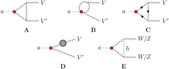
Figure 4: One-loop diagrams contributing to $g_{agg}$, $g_{a\gamma\gamma}$, $g_{a\gamma Z}$, $g_{aZZ}$ and $g_{aWW}$ at one-loop (the corresponding diagrams with Goldstone bosons and the diagrams exchanging the gauge boson legs are left implicit), where $V$ and $V^{\prime}$ are either a gluon, a photon, a $Z$ boson or a $W$ boson. The last diagram only corrects insertions of the $g_{aZZ}$ and $g_{aWW}$ couplings.

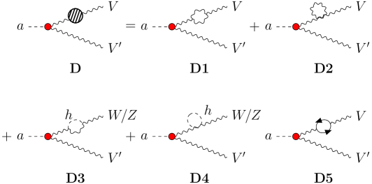
Figure 5: One-loop diagrams contributing to the correction to the external gauge boson legs. Diagrams with Goldstone bosons and Higgs tadpole diagrams are included. Notice that diagrams D3 and D4 are only present for a $Z$ or $W$ boson external legs.

The Feynman diagrams which induce one loop corrections to the effective anomalous ALP coupling to photons, $g_{a\gamma\gamma}$, are depicted in Fig. 4 A, B, C and D, with $V=V^{\prime}=\gamma$ (which implies that $W$ is the gauge boson running in the closed gauge loops, while the virtual gauge boson coupled to $a$ in diagram D is either a photon or a $Z$ boson). Among the four effective electroweak couplings, insertions of the set $\{g_{a\gamma\gamma},g_{aWW},g_{a\gamma Z}\}$ contribute to the one-loop corrected effective coupling $g^{\text{eff}}_{a\gamma\gamma}$. Using the gauge-invariance relations Eq. (36), we choose to express the final result in terms of just two of them, e.g. the set $\{g_{a\gamma\gamma},g_{aWW}\}$, plus fermionic couplings:

$$g_{a\gamma\gamma}^{\text{eff}}= g_{a\gamma\gamma}\left\{1+\frac{\alpha_{em}}{6\pi}\,A^{Z/\gamma\rightarrow\gamma}\right\}+\frac{2\alpha_{em}}{\pi}g_{aWW}B_{2}\left(\frac{4M_{W}^{2}}{p^{2}}\right)-\frac{\alpha_{em}}{\pi f_{a}}\sum_{\text{f}}c_{\text{f}}\,Q_{\text{f}}^{2}N_{C}B_{1}\left(\frac{4m_{\text{f}}^{2}}{p^{2}}\right)\,,$$ (56)

where here and all through the rest of the paper (unless stated otherwise) the sum over fermions denotes all possible individual fermion flavours, $\text{f}=u,c,t,d,s,b,e,\mu,\tau$, and $p$ denotes the 4-momentum of the ALP, $N_{C}$ is the number of colours for a given fermion f (i.e. 3 for quarks and 1 for leptons), $Q_{\text{f}}$ is its electric charge. The functions $B_{1}$ and $B_{2}$ have already been defined in Ref. Bauer:2017ris as:

$$B_{1}(\tau)=1-\tau f^{2}(\tau)\,,\qquad B_{2}(\tau)=1-(\tau-1)f^{2}(\tau)\,,\qquad\mbox{with }f(\tau)=\begin{cases}\arcsin\frac{1}{\sqrt{\tau}}&\mbox{for }\tau\geq 1\\ \frac{\pi}{2}+\frac{i}{2}\ln{\frac{1+\sqrt{1-\tau}}{1-\sqrt{1-\tau}}}&\mbox{for }\tau<1\end{cases}\,.$$ (57)

The function $A^{Z/\gamma\rightarrow\gamma}$ encodes pure leg radiative corrections stemming from diagramas D1, D2 and D5 in Fig. 5 (with the virtual gauge boson attached to $a$ being either a photon or a $Z$ boson, while the $W$ boson runs in the closed gauge loops),

$$A^{Z/\gamma\rightarrow\gamma}= 1-2\sum_{\text{f}}Q_{\text{f}}^{2}N_{C}\log\left(\frac{\Lambda^{2}}{m_{\text{f}}^{2}}\right)+\frac{21}{2}\log\left(\frac{\Lambda^{2}}{M_{W}^{2}}\right)\,.$$ (58)

This computation has been carried out in dimensional regularization, trading next the $1/\epsilon$ UV-divergent terms for an energy cutoff $\Lambda$ via the $\overline{\text{MS}}$ prescription $1/{\epsilon}-\gamma_{E}+\log\left(4\pi\mu^{2}\right)\rightarrow\log\Lambda^{2}$. This leg correction correspond to the SM one-loop redefinition of $\alpha_{em}$. Indeed, were the hatted basis of gauge operators to be used – in which $\alpha_{1}$ and $\alpha_{2}$ enter explicitly in the operators definition (see Eqs. (15) and (38)), the one-loop corrections would read

$$\hat{g}_{a\gamma\gamma}^{\text{eff}}=\,\hat{g}_{a\gamma\gamma}+\frac{2\alpha_{em}}{\pi s_{w}^{2}}\hat{g}_{aWW}B_{2}\left(\frac{4M_{W}^{2}}{p^{2}}\right)-\frac{4}{f_{a}}\sum_{\text{f}}c_{\text{f}}\,Q_{\text{f}}^{2}N_{C}B_{1}\left(\frac{4m_{\text{f}}^{2}}{p^{2}}\right)\,,$$ (59)

a result which in the on-shell ALP limit reduces straightforwardly to that in Ref. Bauer:2017ris .

Eq. (56) could be rewritten if wished in terms of $\{c_{\tilde{B}},c_{\tilde{W}}\}$ (and $c_{\text{f}}$) applying Eq. (32) for $g_{aWW}$ and the last equality in Eq. (53) for $g_{a\gamma\gamma}$ (and analogously for Eq. (59)) .

For an on-shell ALP ($p^{2}=m_{a}^{2}$) the one-loop corrected decay width is simply given by

$$\Gamma(a\rightarrow\gamma\gamma)=\frac{m_{a}^{3}|g_{a\gamma\gamma}^{\text{eff}}|^{2}}{64\pi}\,,$$ (60)

or the equivalent expression in the hat basis with the replacement $g_{a\gamma\gamma}^{\text{eff}}\rightarrow\alpha_{em}/4\pi\,\hat{g}_{a\gamma\gamma}^{\text{eff}}$. We show next some limits of the exact results above for the functions $B_{1}$ and $B_{2}$, for an off-shell ALP, which are of interest in particular experimental contexts.

4.1.1 $g^{\text{eff}}_{a\gamma\gamma}$ for high, intermediate and low ALP $p^{2}$

• For $p^{2}\rightarrow\infty$ ($p^{2}\gg(m_{\text{f}}^{2},M_{Z}^{2},M_{W}^{2})$), only the anomaly contribution remains from fermion coupling insertions. These contributions and those from $g_{aWW}$ insertions reduce to, respectively,

  $$B_{1}=1\,,\qquad B_{2}=-\frac{1}{4}\left(\log\left(\frac{M_{W}^{2}}{p^{2}}\right)+i\pi\right)^{2}\,.$$ (61)

• For intermediate values of $p^{2}$ ($m_{\text{f}}^{2}\ll p^{2}\ll(M_{Z}^{2},M_{W}^{2})\ll m_{t}^{2}$), i.e. smaller than the top and all gauge bosons masses but larger than all other fermion masses, it results

  $$B_{1}=\begin{cases}1\,,&\text{for light fermion insertions: }m_{\text{f}}^{2}\ll p^{2}\ll M_{Z}^{2}\,,\\ 0\,,&\text{for top quark insertion: }p^{2}\ll M_{Z}^{2}\ll m_{t}^{2}\,,\end{cases}\qquad\qquad B_{2}=0\,.$$ (62)

• For $p^{2}\rightarrow 0$, i.e. smaller than all fermion masses, both functions vanish $B_{1}=B_{2}=0$.

4.2 ALP anomalous coupling to gluons

The Feynman diagrams which induce one loop corrections to the effective anomalous coupling of an ALP to two gluons, $g_{agg}$, are depicted by diagrams A, B, C and D of Fig. 4 with $V=V^{\prime}=g$ (which implies that all virtual gauge bosons are also gluons). Only the ALP-quark couplings $c_{\text{f}}$, and $g_{agg}$ itself, can contribute at one-loop to the $g^{\text{eff}}_{gaa}$ amplitude,

$$g_{agg}^{\text{eff}}= g_{agg}\left\{1+\frac{\alpha_{s}}{12\pi}\,G^{gg}\right\}-\frac{\alpha_{s}}{2\pi f_{a}}\sum_{\begin{subarray}{c}\text{f}=u,c,t,\\ d,s,b\end{subarray}}c_{\text{f}}\,B_{1}\left(\frac{4m_{\text{f}}^{2}}{p^{2}}\right)\,,$$ (63)

where $B_{1}$ was defined in Eq. (57), and the function $G^{gg}$ encodes the corrections stemming from the vertex diagram A in Fig. 4 plus those from external leg corrections in diagrams D1, D2 and D5 of Fig. 5.

We have performed the computation of $g_{agg}^{\text{eff}}$ in the $R_{\xi}$ gauge and using dimensional regularization. The latter respects gauge invariance and regulates both ultraviolet (UV) and infrared (IR) divergences when present, portraying both as poles in $1/\epsilon$ and thus mixing them. It is possible to separate UV and IR divergences, though, via the implementation as a previous step of any IR regularization procedure HeinrichLectures –e.g. setting the external gluons off-shell or using an effective gluon “mass” – so as to identify first the UV divergences, and then using this information on the complete pure dimensional regularization result. We obtain,

$$G^{gg}=\, -2\sum_{\begin{subarray}{c}\text{f}=u,c,t,\\ d,s,b\end{subarray}}\left(\frac{1}{\epsilon_{\text{UV}}}-\gamma_{E}+\log\left(\frac{4\pi\mu^{2}_{\text{UV}}}{m_{\text{f}}^{2}}\right)\right)+33\left(\frac{1}{\epsilon_{\text{UV}}}-\gamma_{E}+\log\left(\frac{4\pi\mu^{2}_{\text{UV}}}{p^{2}}\right)\right)$$

$$-9\left(\frac{1}{\epsilon_{\text{IR}}}-\gamma_{E}+\log\left(-\frac{4\pi\mu^{2}_{\text{IR}}}{p^{2}}\right)\right)^{2}\,-33\left(\frac{1}{\epsilon_{\text{IR}}}-\gamma_{E}+\log\left(\frac{4\pi\mu^{2}_{\text{IR}}}{p^{2}}\right)\right)+36+\frac{3\pi^{2}}{2}\,,$$ (64)

where $\epsilon_{\text{UV}}$ ($\epsilon_{\text{IR}}$) and $\mu^{2}_{\text{UV}}$ ($\mu^{2}_{\text{IR}}$) account respectively for the UV (IR) divergence and renormalization scale. This result can be rewritten in terms of UV and IR cutoffs via the $\overline{\text{MS}}$ prescription

$$\frac{1}{\epsilon_{\text{UV}}}-\gamma_{E}+\log\left(4\pi\mu^{2}_{\text{UV}}\right)\rightarrow\log\Lambda^{2}\,,$$ (65)

$$\frac{1}{\epsilon_{\text{IR}}}-\gamma_{E}+\log\left(4\pi\mu^{2}_{\text{IR}}\right)\rightarrow\log\lambda^{2}\,,$$ (66)

where $\Lambda$ and $\lambda$ denote respectively the UV and IR energy cut-offs, leading to

$$G^{gg}=33\log\left(\frac{\Lambda^{2}}{p^{2}}\right)-2\sum_{\begin{subarray}{c}\text{f}=u,c,t,\\ d,s,b\end{subarray}}\log\left(\frac{\Lambda^{2}}{m_{\text{f}}^{2}}\right)-33\log\left(\frac{\lambda^{2}}{p^{2}}\right)-9\left(\log\left(\frac{\lambda^{2}}{p^{2}}\right)+i\pi\right)^{2}+36+\frac{3\pi^{2}}{2}\,.$$ (67)

When computing the probability for a given physical processes, the unphysical dependence on IR divergences will cancel with that stemming from soft and/or collinear gluon bremsstrahlung. In turn, the UV-divergent terms in this equation lead to the beta function for $c_{\tilde{G}}$ in Eq. (47).

4.3 ALP anomalous coupling to $Z$ plus photon

The effective $g_{a\gamma Z}$ coupling receives one-loop corrections from the fermion-ALP couplings $c_{\text{f}}$ and from the complete set of electroweak couplings $\{g_{a\gamma\gamma},g_{aWW},g_{aZZ},g_{a\gamma Z}\}$. The relevant Feynman diagrams are those in Figs. 4 and 5 (except diagram E), with the external vector bosons being either photon or $Z$, and with $V\neq V^{\prime}$. In consequence, the gauge boson running in closed gauge loops can only be the $W$ boson, while the virtual boson attached to $a$ in diagrams D1, D2 and D5 is either $Z$ or $\gamma$, and $V^{\prime}=\gamma$ in diagrams D3 and D4.

The results are shown to become $\xi$-independent –as they must– only when the gauge-electroweak parameter space is reduced to three couplings, using Eq. (36). Applying the latter again, the electroweak set can be further reduced to two anomalous electroweak operators, that we choose to be the set $\{g_{a\gamma Z},g_{aWW}\}$. The total result can be summarized as

$$g_{a\gamma Z}^{\text{eff}}= \,g_{a\gamma Z}\,\left\{1+\frac{\alpha_{em}}{12\pi}\,\Big{(}A^{Z/\gamma\rightarrow\gamma}\,+\frac{1}{c_{w}^{2}s_{w}^{2}}\,A^{Z/\gamma\rightarrow Z}\Big{)}\right\}+\frac{\alpha_{em}}{\pi}\frac{c_{w}}{s_{w}}g_{aWW}\,A^{WW}\,+\frac{\alpha_{em}}{\pi c_{w}s_{w}}\sum_{\text{f}}\frac{c_{\text{f}}}{f_{a}}A^{\text{f}}\,,$$ (68)

where the exact expressions for all the functions in this equation can be found in App. C.1, for an off-shell ALP and on-shell external SM particles. They are defined as follows:

• $A^{Z/\gamma\rightarrow\gamma}$ gathers the external leg corrections with a photon as final particle, (Fig. 5 D1-D5 with $V=\gamma$ and $V^{\prime}=Z$). Its expression was given in Eq. (58).

• $A^{Z/\gamma\rightarrow Z}$ encodes the external leg corrections with $Z$ as final particle (Fig. 5 D1-D5 with $V=Z$ and $V^{\prime}=\gamma$). It can be expanded as

  $$A^{Z/\gamma\rightarrow Z}=A_{\text{ferm}}^{Z/\gamma\rightarrow Z}\,+\,A_{\text{Higgs}}^{Z\rightarrow Z}\,+\,A_{\text{gauge}}^{Z/\gamma\rightarrow Z}\,,$$ (69)

  where

  • $A_{\text{ferm}}^{Z/\gamma\rightarrow Z}$ accounts for the SM fermion loop corrections, Fig. 5 D5, see Eq. (158).

  • $A_{\text{Higgs}}^{Z\rightarrow Z}$ encodes Higgs corrections to external legs in Fig. 5 D3 and D4, see Eq. (159).

  • $A_{\text{gauge}}^{Z/\gamma\rightarrow Z}$ gathers the gauge boson corrections to external legs in Fig. 5 D1 and D2 (with $W$ bosons running in the loop), plus the $g_{a\gamma Z}$ component of the corrections stemming from $g_{a\gamma\gamma}$ and $g_{aZZ}$ insertions in Fig. 5 D1-D5, projected on the parameter space $\{g_{a\gamma Z},g_{aWW}\}$, see Eq. (160).

• $A^{WW}$ contains the contributions from direct vertex insertions of $g_{aWW}$ in diagrams A and B of Fig. 4, plus the $g_{aWW}$ component of the corrections stemming from $g_{a\gamma\gamma}$ and $g_{aZZ}$ insertions in Fig. 5 D1-D5 projected on the parameter space $\{g_{a\gamma Z},g_{aWW}\}$, see Eq. (161).

• $A^{\text{f}}$ encodes the fermion triangle correction from diagram C in Fig. 4, see Eq. (162).

Eq. (68) can be rewritten in terms of $\{c_{\tilde{B}},c_{\tilde{W}}\}$ (and $c_{\text{f}}$) applying Eq. (32) for $g_{aWW}$ and the last equality in Eq. (54) for $g_{a\gamma Z}$.

An example of physical process to which the exact results can be directly applied in case $m_{a}<M_{Z}$ is given by the decay width of a $Z$ boson to photon plus ALP,

$$\Gamma(Z\rightarrow a\gamma)=\frac{M_{Z}^{3}|g_{a\gamma Z}^{\text{eff}}|^{2}}{384\pi}\left(1-\frac{m_{a}^{2}}{M_{Z}^{2}}\right)^{3}\,,$$ (70)

while for $m_{a}>M_{Z}$, the ALP decay width into $Z$ plus photon reads

$$\Gamma(a\rightarrow\gamma Z)=\frac{m_{a}^{3}|g_{a\gamma Z}^{\text{eff}}|^{2}}{128\pi}\left(1-\frac{M_{Z}^{2}}{m_{a}^{2}}\right)^{3}\,.$$ (71)

We illustrate next the results obtained above for a generic off-shell ALP in some particular limits of practical interest.

4.3.1 $g^{\text{eff}}_{a\gamma Z}$ for high ALP $p^{2}$

For $p^{2}\rightarrow\infty$, ($p^{2}\gg(m_{\text{f}}^{2},M_{Z}^{2},M_{W}^{2})$), the anomaly contribution yields:

$$A^{\text{f}}=2N_{C}Q_{\text{f}}^{2}s_{w}^{2}\,,$$ (72)

while the correction proportional to $g_{aWW}$ is given by

$$A^{WW}=\frac{42M_{W}^{2}+M_{Z}^{2}}{12M_{W}^{2}}\log\left(\frac{\Lambda^{2}}{M_{W}^{2}}\right)-\sum_{\text{f}}\frac{N_{C}Q_{\text{f}}(T_{3,\text{f}}-2Q_{\text{f}}s_{w}^{2})}{3c_{w}^{2}}\log\left(\frac{\Lambda^{2}}{m_{\text{f}}^{2}}\right)-\left(\log\left(\frac{M_{W}^{2}}{p^{2}}\right)+i\pi\right)^{2}\,,$$ (73)

where the terms proportional to $\log\Lambda$ are kept, because consistency of the EFT expansion requires $p^{2}<\Lambda^{2}$.

4.3.2 $g^{\text{eff}}_{a\gamma Z}$ for intermediate and low ALP $p^{2}$

Both for $m_{\text{f}}^{2}\ll p^{2}\ll(M_{Z}^{2},M_{W}^{2})\ll m_{t}^{2}$, where f refers to all fermion mass but the top one, and for $p^{2}\rightarrow 0$ ($p^{2}\ll(m_{\text{f}}^{2},M_{Z}^{2})$), i.e. smaller than all fermion masses (which can apply for instance to $Z$ decay to ALP + photon), the contribution of fermionic ALP couplings to $g^{\text{eff}}_{a\gamma Z}$ is well approached by

$$A^{\text{f}}=\begin{cases}2N_{C}Q_{\text{f}}^{2}s_{w}^{2}\,,&\text{for light fermions: }m_{\text{f}}^{2}\ll M_{Z}^{2}\,,\\ \frac{3Q_{t}}{2}\,,&\text{for the top quark: }m_{t}^{2}\gg M_{Z}^{2}\,,\end{cases}$$ (74)

while the correction proportional to $g_{aWW}$ reads

$$A^{WW}=\frac{42M_{W}^{2}+M_{Z}^{2}}{12M_{W}^{2}}\log\left(\frac{\Lambda^{2}}{M_{W}^{2}}\right)-\sum_{\text{f}}\frac{N_{C}Q_{\text{f}}(T_{3,\text{f}}-2Q_{\text{f}}s_{w}^{2})}{3c_{w}^{2}}\log\left(\frac{\Lambda^{2}}{m_{\text{f}}^{2}}\right)+...\,,$$ (75)

where dots stand for constant terms.

4.4 ALP anomalous coupling to $ZZ$

The effective $g_{aZZ}$ coupling receives corrections induced by three of the four electroweak gauge couplings: the set $\{g_{aWW},g_{aZZ},g_{a\gamma Z}\}$, plus $\bf{c}_{\text{f}}$ fermion corrections. All Feynman diagrams in Figs. 4 and 5 contribute with $V=V^{\prime}=Z$. Using Eq. (36), the contributions resulting from electroweak gauge insertions can be projected on a two-dimensional space of couplings, which we choose to be here $\{g_{aZZ},g_{aWW}\}$. The total effective coupling $g_{aZZ}$ can then be expressed as

$$g_{aZZ}^{\text{eff}}= g_{aZZ}\left\{1+\frac{\alpha_{em}}{6\pi c_{w}^{2}s_{w}^{2}}\,(A^{Z/\gamma\rightarrow Z}+B^{\text{Higgs}})\right\}+\frac{\alpha_{em}}{\pi}\frac{c_{w}^{2}}{s_{w}^{2}}g_{aWW}B^{WW}+\frac{\alpha_{em}}{\pi c_{w}^{2}s_{w}^{2}}\sum_{\text{f}}\frac{c_{\text{f}}}{f_{a}}B^{\text{f}}\,,$$ (76)

where the complete expressions for the functions in this expression can be found in App. C.2. They correspond to:

• $A^{Z/\gamma\rightarrow Z}$ encodes corrections to the external legs (diagrams D1-D5 in Fig. 5), see Eq. (158) for the exact result.

• $B^{\text{Higgs}}$ stems from the vertex insertion of $g_{aZZ}$ with a Higgs particle exchanged between the two $Z$ bosons (diagram E in Fig. 4), see Eq. (167).

• $B^{WW}$ collects the contributions proportional to $g_{aWW}$ resulting from direct vertex insertions of $g_{aWW}$ in Fig.4 A and B, plus the $g_{aWW}$ component of the contributions seeded by the insertion of $g_{a\gamma Z}$ in the external legs and then projected onto the parameter space $\{g_{aZZ},g_{aWW}\}$, see Eq. (168).

• Finally, the function $B^{\text{f}}$ encodes the contributions from vertex insertions of the fermionic couplings $c_{\text{f}}$ (Fig. 4 C), see Eq. (169).

Eq. (76) can be rewritten in terms of $\{c_{\tilde{B}},c_{\tilde{W}}\}$ (and $c_{\text{f}}$) applying Eq. (32) for $g_{aWW}$ and the last equality in Eq. (55) for $g_{aZZ}$.

The results in this subsection can be applied to a variety of transitions in which the ALP may be on-shell or off-shell. For instance, for $m_{a}>2M_{Z}$ the one-loop corrected ALP decay width into two $Z$ bosons is simply given by

$$\Gamma(a\rightarrow ZZ)=\frac{m_{a}^{3}|g_{aZZ}^{\text{eff}}|^{2}}{64\pi}\left(1-\frac{4M_{Z}^{2}}{m_{a}^{2}}\right)^{3/2}\,.$$ (77)

We present next for illustration the limit of the complete results in App. C.2 in the particular case of high ALP four-momentum squared, which can be of interest for instance for non-resonant collider ALP searches.

4.4.1 $g^{\text{eff}}_{aZZ}$ for high ALP $p^{2}$

For $p^{2}\rightarrow\infty$ ($p^{2}\gg(m_{\text{f}}^{2},M_{Z}^{2},M_{W}^{2})$), only the anomaly contribution remains from the insertion of ALP-fermions couplings,

$$B^{\text{f}}=-N_{C}Q_{\text{f}}^{2}s_{w}^{4}\,,$$ (78)

while the contribution proportional to $g_{aWW}$ simplifies to

$$B^{WW}=\frac{42M_{W}^{2}+M_{Z}^{2}}{12M_{W}^{2}}\log\left(\frac{\Lambda^{2}}{M_{W}^{2}}\right)-\sum_{\text{f}}\frac{N_{C}Q_{\text{f}}(T_{3,\text{f}}-2Q_{\text{f}}s_{w}^{2})}{3c_{w}^{2}}\log\left(\frac{\Lambda^{2}}{m_{\text{f}}^{2}}\right)-\frac{1}{2}\left(\log\left(\frac{M_{W}^{2}}{p^{2}}\right)+i\pi\right)^{2}\,,$$ (79)

and that proportional to $g_{aZZ}$ corrected by Higgs boson exchange between external legs vanishes, $B^{\text{Higgs}}=0$.

4.5 ALP anomalous coupling to $W^{+}W^{-}$

All four couplings in the ensemble $\{g_{a\gamma\gamma},g_{aWW},g_{aZZ},g_{a\gamma Z}\}$ induce one-loop corrections to the effective $g^{\text{eff}}_{aWW}$ coupling. All Feynman diagrams in Figs. 4 and 5 contribute. The complete results can be found in App. C.3. Using Eq. (36), the total result can be expressed for instance as a function of $\{g_{aWW},g_{a\gamma\gamma}\}$ plus fermionic couplings,

$$g_{aWW}^{\text{eff}}= g_{aWW}\Bigg{\{}1+\frac{\alpha_{em}}{24\pi s_{w}^{2}}(A^{W\rightarrow W}+C^{WW}+C^{\text{Higgs}})\Bigg{\}}+\frac{\alpha_{em}}{2\pi}g_{a\gamma\gamma}\,C^{\gamma\gamma}+\frac{\alpha_{em}}{\pi s_{w}^{2}}\sum_{\text{f}}\frac{c_{\text{f}}}{f_{a}}C^{\text{f}}\,,$$ (80)

where:

• $A^{W\rightarrow W}$ contains two sources of one-loop external-leg SM corrections to the insertion of $g_{aWW}$ itself: fermionic and Higgs corrections,

  $$A^{W\rightarrow W}=A^{W\rightarrow W}_{\text{ferm}}+A^{W\rightarrow W}_{\text{Higgs}}\,,$$ (81)

  with only fermion doublets contributing to $A^{W\rightarrow W}_{\text{ferm}}$, see diagram D5 in Fig. 5 and Eq. (174), and the Higgs-dependent term $A^{W\rightarrow W}_{\text{Higgs}}$ stemming from diagrams D3 and D4 in Fig. 5, see Eq. (175).

• $C^{WW}$ accounts for corrections proportional to $g_{aWW}$, and gathers one-loop SM corrections on the external legs (Fig. 5 D1 and D2) together with vertex ones (Fig. 4 A and B) (see Eq. (176) for the complete expression):

  • The leg corrections and those from the vertex diagram B are directly seeded by the insertion of $g_{aWW}$.

  • The contributions originated from diagram A correspond to the combination of direct vertex insertions of $g_{aWW}$, plus the $g_{aWW}$ component of the contributions seeded by $\{g_{aZZ},g_{a\gamma Z}\}$ insertions projected onto the $\{g_{a\gamma\gamma},g_{aWW}\}$ parameter space.

• $C^{\text{Higgs}}$ is a pure vertex correction resulting from the direct insertion of $g_{aWW}$ with the Higgs boson exchanged between the two $W$ legs (diagram E in Fig. 4), see Eq. (177).

• The vertex function $C^{\gamma\gamma}$ corresponds to Fig. 4 A, combining the results from the direct insertion of $g_{a\gamma\gamma}$ and the $g_{a\gamma\gamma}$ component of the contributions seeded by $\{g_{a\gamma Z},g_{aZZ}\}$ insertions projected onto the $\{g_{\gamma\gamma},g_{aWW}\}$ parameter space, see Eq. (178).

• Finally, the vertex function $C^{\text{f}}$ accounts for the fermionic triangle contributions (Fig. 4 C), induced by fermionic couplings $c_{\text{f}}$ insertions, see Eq. (179).

Eq. (80) can be rewritten in terms of $\{c_{\tilde{B}},c_{\tilde{W}}\}$ (and $c_{\text{f}}$) applying Eq. (32) for $g_{aWW}$ and the last equality in Eq. (53) for $g_{a\gamma\gamma}$.

We present next for illustration the high ALP four-momentum squared limit of the functions in Eq. (80).

4.5.1 $g^{\text{eff}}_{aWW}$ for high ALP $p^{2}$

In the limit $p^{2}\rightarrow\infty$ ($p^{2}\gg(m_{\text{f}}^{2},M_{Z}^{2},M_{W}^{2})$), the fermionic contribution to the anomaly vanishes. The same holds in this limit for the correction proportional to $g_{a\gamma\gamma}$ as well as that stemming from Higgs boson-exchange between the external $W$ bosons,

$$C^{\text{f}}=C^{\gamma\gamma}=C^{\text{Higgs}}=0\,.$$ (82)

The only non-vanishing contributions in this limit are those proportional to $g_{aWW}$ itself and stemming from $A^{W\rightarrow W}$ and $C^{WW}$. The function $A^{W\rightarrow W}$ is independent of $p^{2}$: in consequence, it is not further simplifed from the relatively cumbersome complete expressions in Eqs. (174) and Eq. (175), see Eq. (161). The function $C^{WW}$ simplifies to

$$C^{WW}=43\log\left(\frac{\Lambda^{2}}{M_{W}^{2}}\right)-12\left(\log\left(\frac{M_{W}^{2}}{p^{2}}\right)+i\pi\right)^{2}-12s_{w}^{2}\log\left(\frac{\lambda^{2}}{M_{W}^{2}}\right)\left(1+i\pi+\log\left(\frac{M_{W}^{2}}{p^{2}}\right)\right)...\,,$$ (83)

where $\Lambda$ is the UV cutoff (this logarithmic dependence cannot be disregarded in front of that in $p^{2}$ for EFT consistency), and $\lambda$ denotes the IR cutoff. The computation has been carried out entirely in dimensional regularization, with the $1/\epsilon$ terms traded next for energy cutoffs via a protocol alike to that used for $g^{\text{eff}}_{agg}$ –Eq. (4.2)– and the prescription in Eq. (65). The $\log\Lambda$ dependence contained in $C^{WW}$ combined with that in the leg correction $A^{W\rightarrow W}$ determines the beta function for $c_{\tilde{W}}$ in Eq. (46).

The two first terms in Eq. (83) are the leading contributions for large enough $p^{2}$. The third term exhibits a logarithimic dependence on the IR cutoff which is instead physically irrelevant and can be disregarded, as it will exactly cancel for any physical observable against the contributions from soft and/or collinear photon brehmsstrahlung. The latter may also contribute additional finite terms to be combined with the finite and $p^{2}$ independent terms in $C^{WW}$ (see the exact expression in Eq. (176) in App. C.3), encoded here by dots.

For intermediate ($m_{\text{f}}^{2}\ll p^{2}\ll(M_{Z}^{2},M_{W}^{2})\ll m_{t}^{2}$) and low ($p^{2}\ll(m_{\text{f}}^{2},M_{Z}^{2})$) ALP four-momentum, the ALP-$WW$ transition is again not kinematically possible for gauge bosons on-shell.

4.6 ALP fermionic couplings

The one-loop corrections to the effective ALP-fermion-fermion couplings are depicted in Figs. 6 and 7, where the internal wavy lines denote either the gluon in the case of the gluon-ALP coupling $g_{agg}$ (only possible for quark final states) or electroweak gauge bosons. Contrary to the case for all previous effective couplings described, the individual contributions seeded by each of the electroweak couplings in the set $\{g_{a\gamma\gamma},g_{aWW},g_{aZZ},g_{a\gamma Z}\}$ are separately gauge invariant. In other words, the $\xi$-independence of the results holds already at the level of each one of those contributions, that is, prior to their projection onto a reduced parameter space of electroweak gauge couplings. For this reason, we will present those contributions individually. If wished, the reader can trivially project those results in the two-coupling $\{c_{\tilde{W}},c_{\tilde{B}}\}$ parameter space, or on any other parameter space (e.g. $\{g_{a\gamma\gamma},{g_{aWW}}\}$), using the gauge-invariance relations in Eq. (36).

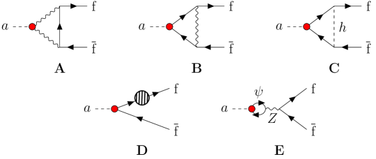
Figure 6: One-loop diagrams contributing to $c_{\text{f}}$ at one-loop (plus the corresponding diagrams with Goldstone bosons). The wavy lines denote gauge bosons: gluons, photons, $W$ and $Z$ bosons.

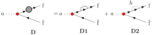
Figure 7: One-loop diagrams contributing to the correction to the external fermion legs. Diagrams with Goldstone bosons are included.

The results can be summarized as

$$\frac{c_{\text{f}}^{\text{eff}}}{f_{a}}= \frac{c_{\text{f}}}{f_{a}}\left\{1+\frac{\alpha_{em}}{2\pi}\,D^{c_{\text{f}}}+\frac{\alpha_{s}}{3\pi}\,D^{c_{\text{f}}}_{g}\right\}+\frac{\alpha_{em}}{2\pi f_{a}}\,\big{\{}c_{\text{f'}}\,D^{c_{\text{f'}}}+\sum_{\psi}{c_{\psi}}\,\,D^{c_{\psi}}_{\text{mix}}\big{\}}$$ (84)

$$+ \frac{\alpha_{em}}{2\pi}\left\{g_{a\gamma\gamma}\,D^{\gamma\gamma}+g_{a\gamma Z}\,D^{\gamma Z}+g_{aZZ}\,D^{ZZ}+g_{aWW}\,D^{WW}\right\}+\frac{\alpha_{s}}{3\pi}\left\{g_{agg}\,D^{gg}\right\}\,,$$

where the sum over fermions runs over all possible flavours, $\psi=u,c,t,d,s,b,e,\mu,\tau$, and the terms in the second line account –respectively– for vertex insertions of the phenomenological ALP electroweak couplings $\{g_{a\gamma\gamma},g_{a\gamma Z},g_{aZZ},g_{aWW}\}$ plus the anomalous gluon coupling $g_{agg}$: they all stem from diagram A in Fig. 6, and each term is separately gauge invariant. The complete expressions for the functions $D^{\gamma\gamma}$, $D^{\gamma Z}$, $D^{ZZ}$ and $D^{WW}$ can be found in Eqs. (180)-(184) of App. C.4. The first line in Eq. (84) encodes instead insertions of:

• The fermionic coupling $c_{\text{f}}$ itself accompanied by one-loop exchange of a gluon, encoded in $D^{c_{\text{f}}}_{g}$, or by the one-loop exchange of either a photon, a $Z$, a $W$ or a Higgs boson, i.e.

  $$D^{c_{\text{f}}}=D^{c_{\text{f}}}_{\gamma}+D^{c_{\text{f}}}_{Z}+D^{c_{\text{f}}}_{W}+D^{c_{\text{f}}}_{h}\,,$$ (85)

  where $D^{c_{\text{f}}}_{W}$ is a pure leg correction from $W$ exchange (Fig. 7 D1), and it is $\xi$-independent by itself, see Eq. (188). In contrast, in to order get results in an explicitly gauge invariant formulation, the one-loop corrections due to photon or $Z$ exchange –encoded respectively in $D^{c_{\text{f}}}_{\gamma}$ and $D^{c_{\text{f}}}_{Z}$– require the combination of the vertex diagram B in Fig. 6 and the leg correction in Fig. 7 D1, see Eqs. (186) and (187). Similarly, manifest gauge invariance of the Higgs-exchange corrections –encoded in $D^{c_{\text{f}}}_{h}$– results after combining the vertex correction in Fig. 6 C and the leg corrections in Fig. 7 D2, see Eq. (190).

• The contribution from $c_{\text{f'}}$, where f’ denotes the $SU(2)_{L}$ flavour partner of fermion f, encoded in the function $D^{c_{\text{f'}}}$ given in Eq. (189). It corresponds to the vertex correction due to $W$ exchange in Fig. 6 B, which is gauge invariant by itself.

• All possible fermionic contributions to the mixed $a$-$Z$ correction in Fig. 6 E, which are encoded through the functions $D^{c_{\psi}}_{\text{mix}}$, which are also separately gauge-invariant, see the complete result in Eq. (191).

The results can be applied to a variety of physical transitions with an ALP on- or off-shell. For instance, for ALP decay into a fermionic $\text{f}\bar{\text{f}}$ channel when $m_{a}>2\,m_{\text{f}}$, the one-loop corrected width is simply obtained from

$$\Gamma(a\rightarrow\text{f}\,\bar{\text{f}})=\frac{N_{C}m_{a}m_{\text{f}}^{2}|c_{\text{f}}^{\text{eff}}|^{2}}{8\pi f_{a}^{2}}\sqrt{1-\frac{4m_{\text{f}}^{2}}{m_{a}^{2}}}\,.$$ (86)

For simplicity and for illustration purposes, we present next in this subsection some useful limits of the exact functions in App. C.4, for a generic off-shell ALP.

4.7 ${c_{\text{f}}^{\text{eff}}}$ for high ALP $p^{2}$

For non-resonant searches at the LHC and other colliders, and/or for very heavy ALPs, the limit $m_{\text{f}}^{2}\ll(M_{Z}^{2},M_{W}^{2},M_{H}^{2})\ll m_{t}^{2}\ll p^{2}$ is of physical interest, where $m_{\text{f}}$ refers to all fermion masses but the top one. In this subsection we set $m_{\text{f}}=0$ except in divergent terms.

4.7.1 Limit of light external fermions for ${\text{f}=u,d,s,b,e,\mu}$

Let us first consider the contribution of gauge-anomalous couplings to ${c_{\text{f}}^{\text{eff}}}$. For instance, $D^{gg}$ encodes the $g_{agg}$ contribution with gluons running in the internal loop of diagram A in Fig. 6, which in this limit reduces to

$$D^{gg}=\Bigg{\{}3\log\left(\frac{\Lambda^{2}}{m_{\text{f}}^{2}}\right)-4-\frac{2\pi^{2}}{3}-\frac{1}{2}\left(\log\left(\frac{m_{\text{f}}^{2}}{p^{2}}\right)+i\pi\right)^{2}\Bigg{\}}\,.$$ (87)

Analogously, $D^{\gamma\gamma}$ accounts for the $g_{a\gamma\gamma}$ insertion with two photons running in the internal loop of diagram A in Fig. 6, with an expression very close to that of $D^{gg}$ which in this limit reduces to

$$D^{\gamma\gamma}=\frac{Q_{\text{f}}^{2}}{2}D^{gg}\,,$$ (88)

while the $D^{\gamma Z}$ term stems from that same diagram with one photon and one $Z$ boson in the internal loop,

$$D^{\gamma Z}=\frac{Q_{\text{f}}\,(T_{3,\text{f}}-2Q_{\text{f}}s_{w}^{2})}{16c_{w}s_{w}}\Bigg{\{}12\log\left(\frac{\Lambda^{2}}{M_{Z}^{2}}\right)-19-\frac{2\pi^{2}}{3}-2\left(\log\left(\frac{M_{Z}^{2}}{p^{2}}\right)+i\pi\right)^{2}$$ (89)

$$-\log\left(\frac{m_{\text{f}}^{2}}{M_{Z}^{2}}\right)\left[6+4i\pi+4\log\left(\frac{M_{Z}^{2}}{p^{2}}\right)\right]\Bigg{\}}\,.$$ (90)

Similarly, the same diagram in Fig. 6 A although with two internal $Z$ bosons results in

$$D^{ZZ}=\frac{1}{8c_{w}^{2}s_{w}^{2}}\Bigg{\{}(T_{3,\text{f}}^{2}-2T_{3,\text{f}}Q_{\text{f}}s_{w}^{2}+2Q_{t}s_{w}^{4})\left(6\log\left(\frac{\Lambda^{2}}{M_{Z}^{2}}\right)-11\right)$$ (91)

$$+4T_{3,\text{f}}^{2}\left(1+\log\left(\frac{M_{Z}^{2}}{p^{2}}\right)+i\pi\right)+4Q_{\text{f}}^{2}s_{w}^{2}(T_{3,\text{f}}-Q_{\text{f}}s_{w}^{2})\left(\log\left(\frac{M_{Z}^{2}}{p^{2}}\right)+i\pi\right)^{2}\Bigg{\}}\,,$$ (92)

while $D^{WW}$ corresponds to that same diagram, albeit with internal W bosons,

$$D^{WW}=\begin{cases}\frac{1}{16s_{w}^{2}}\Bigg{\{}6\log\left(\frac{\Lambda^{2}}{p^{2}}\right)-2\log\left(\frac{M_{W}^{2}}{p^{2}}\right)-7+4i\pi\Bigg{\}}\,,&\begin{aligned} &\text{for leptons and quarks}\\ &\text{except top and bottom}\,,\end{aligned}\\ \frac{1}{16s_{w}^{2}}\Bigg{\{}6\log\left(\frac{\Lambda^{2}}{p^{2}}\right)-2\log\left(\frac{m_{t}^{2}}{p^{2}}\right)-9+4i\pi\Bigg{\}}\,,&\text{for the bottom quark}\,.\end{cases}$$ (93)

For the contributions resulting from the insertions of ALP fermionic couplings, the one-loop gluon corrections (vertex plus legs), and the analogous one-loop photon corrections lead in this limit to, respectively,

$$D^{c_{\text{f}}}_{g}=-2\Bigg{\{}1-\frac{\pi^{2}}{6}+\log\left(\frac{\lambda^{2}}{m_{\text{f}}^{2}}\right)\left(1+i\pi+\log\left(\frac{m_{\text{f}}^{2}}{p^{2}}\right)\right)+\frac{1}{2}\left(\log\left(\frac{m_{\text{f}}^{2}}{p^{2}}\right)+i\pi\right)^{2}\Bigg{\}}\,,$$ (94)

$$D^{c_{\text{f}}}_{\gamma}=\frac{Q_{\text{f}}^{2}}{2}\,D^{c_{\text{f}}}_{g}\,,$$ (95)

where $\lambda$ is an infrared cutoff which encodes the IR-divergent contributions to the $1/\epsilon$ dimensional regularization terms via the prescription in Eq. (65), following the same protocol used for the gluonic IR divergences in Eq. (4.2). and the photonic ones in Eq. (83). Those unphysical IR logarithmic dependences will again exactly cancel in physical transitions against those from the phase space integral terms stemming from tree-level soft and/or collinear gluon and photon bremsstrahlung.

In turn, $Z$ exchange (vertex plus legs) is free from IR divergences and leads to

$$D^{c_{\text{f}}}_{Z}=-\frac{Q_{\text{f}}s_{w}^{2}(T_{3,\text{f}}-Q_{\text{f}}s_{w}^{2})}{2c_{w}^{2}s_{w}^{2}}\Bigg{\{}\frac{2\pi^{2}}{3}+\left(\log\left(\frac{M_{Z}^{2}}{p^{2}}\right)+i\pi\right)^{2}\Bigg{\}}\,.$$ (96)

The ${c_{\text{f}}^{\text{eff}}}$ component resulting from one-loop $W$-exchange corrections to ALP fermion-coupling insertions unfolds as explained as two $\xi$-independent contributions: i) the leg correction from the insertion of $c_{\text{f}}$ in Fig. 7 D1, encoded in $D^{c_{\text{f}}}_{W}$, which in this particular limit vanishes, and ii) the vertex correction induced by the insertion of the $SU(2)$ flavour-partner coupling $c_{\text{f}^{\prime}}$ in Fig. 6 B, encoded in $D^{c_{\text{f'}}}$:

$$D^{c_{\text{f'}}}=\begin{cases}0\,,&\begin{aligned} &\text{for leptons and quarks}\\ &\text{except top and bottom}\,,\end{aligned}\\ -\frac{m_{t}^{2}}{8M_{W}^{2}s_{w}^{2}}\Bigg{\{}\log\left(\frac{\Lambda^{2}}{p^{2}}\right)+\log\left(\frac{M_{W}^{2}}{p^{2}}\right)+\frac{7}{2}+2i\pi\Bigg{\}}\,,&\text{for the bottom quark}\,.\end{cases}\,.$$ (97)

The one-loop Higgs corrections to $c_{\text{f}}$ insertions also vanish in this limit, $D^{c_{\text{f}}}_{h}=0$. Finally, the mixed one-loop contribution to $c_{\text{f}}^{\text{eff}}$ from diagram E in Fig. 6 receives contributions from all possible ALP fermionic couplings –quarks and leptons, and it is also $\xi$-independent by itself. Its expression is particularly simple even in the exact case (see Eq. (191) in App. C), while in the present limit all contributions vanish but for that with the top quark running in the loop,

$$D^{c_{t}}_{\text{mix}}=-\frac{3T_{3,\text{f}}\,m_{t}^{2}}{2s_{w}^{2}M_{W}^{2}}\Bigg{\{}\log\left(\frac{\Lambda^{2}}{p^{2}}\right)+2+i\pi\Bigg{\}}\,,$$ (98)

where $T_{3,\text{f}}$ denotes the third component of weak isospin for the external flavour f. The logarithimic dependence was already obtained in Ref. Feng:1997tn . This result shows that, in the limit under study, the top-coupling contribution can be the dominant one on the quest for signals of ALP couplings to light fermions, because the contributions are proportional to the mass of the fermion running in the loop and independent of the external flavour. In fact, this conclusion extends as well to the exact result in Eq. (191). This may be very relevant for instance on the searches for ALP couplings to electrons in XENON and other experiments, see Sec. 6.

4.7.2 Limit of light internal fermions for external $\text{f}=t$

The analogous high ALP $p^{2}$ results when the external fermion is the top, i.e. the contributions to ${c_{t}^{\text{eff}}}$ neglecting light fermion masses, are reported next.

Let us consider first the impact of the insertions of ALP gauge anomalous couplings. In the case of the ALP-photon and ALP-gluon couplings, $g_{agg}$ and $g_{a\gamma\gamma}$, the corresponding functions $D^{gg}$ and $D^{\gamma\gamma}$ are exactly as those in Eqs. (87) and (88) albeit with the replacement $m_{\text{f}}\rightarrow m_{t}$. For the other anomalous couplings, the results simplify to

$$D^{\gamma Z}=\frac{Q_{t}\,(T_{3,t}-2Q_{t}s_{w}^{2})}{4c_{w}s_{w}}\Bigg{\{}3\log\left(\frac{\Lambda^{2}}{m_{t}^{2}}\right)-4\Bigg{\}}\,,$$ (99)

$$D^{ZZ}=\frac{1}{4c_{w}^{2}s_{w}^{2}}\Bigg{\{}(T_{3,t}^{2}-2T_{3,t}Q_{t}s_{w}^{2}+2Q_{t}s_{w}^{4})\left(3\log\left(\frac{\Lambda^{2}}{m_{t}^{2}}\right)-4\right)$$ (100)

$$+2Q_{t}^{2}s_{w}^{2}(T_{3,t}-Q_{t}s_{w}^{2})\Bigg{[}\frac{2\pi^{2}}{3}+\frac{1}{2}\left(\log\left(\frac{m_{t}^{2}}{p^{2}}\right)+i\pi\right)^{2}\Bigg{]}+2T_{3,t}^{2}\left(\log\left(\frac{m_{t}^{2}}{p^{2}}\right)+i\pi\right)\Bigg{\}}\,,$$ (101)

$$D^{WW}=\frac{1}{8s_{w}^{2}}\Bigg{\{}3\log\left(\frac{\Lambda^{2}}{p^{2}}\right)-\log\left(\frac{m_{t}^{2}}{p^{2}}\right)-3+3i\pi\Bigg{\}}\,.$$ (102)

In turn, the one-loop gluon and photon contributions to ${c_{t}^{\text{eff}}}$ stemming from ALP-fermion couplings, i.e. $D^{c_{\text{f}}}_{g}$ and $D^{c_{\text{f}}}_{\gamma}$, are respectively identical to those found above for the light external fermion limit in Eqs. (94) and (95). The rest of the one-loop boson corrections to insertions of ALP-fermion couplings reads in this limit:

$$D^{c_{t}}_{Z}=\frac{1}{2c_{w}^{2}s_{w}^{2}}\Bigg{\{}-\frac{m_{t}^{2}T_{3,t}^{2}}{M_{Z}^{2}}\left(\log\left(\frac{\Lambda^{2}}{p^{2}}\right)+2+i\pi\right)-(T_{3,t}^{2}+4T_{3,t}Q_{t}s_{w}^{2}-4Q_{t}^{2}s_{w}^{4})\log\left(\frac{m_{t}^{2}}{M_{Z}^{2}}\right)$$ (103)

$$-Q_{t}s_{w}^{2}(T_{3,t}-Q_{t}s_{w}^{2})\left[\frac{\pi^{2}}{3}+2\log\left(\frac{m_{t}^{2}}{M_{Z}^{2}}\right)\left(\log\left(\frac{m_{t}^{2}}{p^{2}}\right)+i\pi\right)-\left(\log\left(\frac{m_{t}^{2}}{p^{2}}\right)+i\pi\right)^{2}\right]\Bigg{\}}\,,$$

$$D^{c_{t}}_{W}=-\frac{m_{t}^{2}}{8M_{W}^{2}s_{w}^{2}}\Bigg{\{}\log\left(\frac{\Lambda^{2}}{m_{t}^{2}}\right)+1+i\pi\Bigg{\}}\,,$$ (104)

$$D^{c_{t}}_{h}=-\frac{m_{t}^{2}}{8\pi s_{w}^{2}M_{W}^{2}}\Bigg{\{}\log\left(\frac{\Lambda^{2}}{M_{H}^{2}}\right)+\log\left(\frac{p^{2}}{M_{H}^{2}}\right)-2-i\pi\Bigg{\}}\,,$$ (105)

$$D^{c_{\psi}}_{\text{mix}}=-\frac{3m_{t}^{2}}{4s_{w}^{2}M_{W}^{2}}\Bigg{\{}\log\left(\frac{\Lambda^{2}}{m_{t}^{2}}\right)+2+i\pi\Bigg{\}}\,,$$ (106)

while $D^{c_{\text{f'}}}_{W}=0$ with $\text{f'}=b$ in this particular case.

4.8 ${c_{\text{f}}^{\text{eff}}}$ for intermediate ALP $p^{2}$ and light fermions

We explicit now the limits for an ALP with a low $p^{2}$, smaller or equal than all SM boson gauge boson masses but larger than the mass squared of all light fermions $m_{\text{f}}^{2}\ll p^{2}\ll M_{Z}^{2},M_{W}^{2},M_{H}^{2}$ with $\text{f}=u,d,c,s,b,e,\mu,\tau$. This limit is of interest for instance when considering decays of a light ALP to leptons or light fermions, such as those searched for in rare decays.

The contribution stemming from the insertions of $g_{agg}$ and $g_{a\gamma\gamma}$, i.e. the functions $D^{gg}$ and $D^{\gamma\gamma}$, are again exactly as those in Eqs. (87) and (88). For the other anomalous couplings, the results simplify in this limit to

$$D^{\gamma Z}=\frac{Q_{\text{f}}\,(T_{3,\text{f}}-2Q_{\text{f}}s_{w}^{2})}{8c_{w}s_{w}}\Bigg{\{}6\log\left(\frac{\Lambda^{2}}{M_{Z}^{2}}\right)-13\Bigg{\}}\,,$$ (107)

$$D^{ZZ}=\frac{(T_{3,\text{f}}^{2}-T_{3,\text{f}}2Q_{\text{f}}s_{w}^{2}+2Q_{\text{f}}s_{w}^{4})}{8c_{w}^{2}s_{w}^{2}}\Bigg{\{}6\log\left(\frac{\Lambda^{2}}{M_{Z}^{2}}\right)-19\Bigg{\}}\,,$$ (108)

$$D^{WW}=\frac{1}{16s_{w}^{2}}\Bigg{\{}6\log\left(\frac{\Lambda^{2}}{M_{Z}^{2}}\right)-19\Bigg{\}}\,.$$ (109)

The results for $D^{\gamma\gamma}$ and Eqs. (107)-(109) have been addressed previously in Ref. Bauer:2017ris for an on-shell ALP ($p^{2}=m_{a}^{2}$); our results are in agreement with those, except for a minor factor in $D^{\gamma\gamma}$, Eq. (88).

We consider next the impact of inserting ALP fermionic couplings. Their contributions vanish in this particular limit for the following functions:

$$D^{c_{\text{f}}}_{Z}=D^{c_{\text{f}}}_{W}=D^{c_{\text{f}}^{\prime}}_{W}=D^{c_{\text{f}}}_{h}=0\,,$$ (110)

while the gluon and photon corrections $D^{c_{\text{f}}}_{g}$ and $D^{c_{\text{f}}}_{\gamma}$ coincide with those in Eqs. (94) and (95). Finally, the $a$-$Z$ mixing corrections read in this limit Feng:1997tn

$$D^{c_{t}}_{\text{mix}}=-\frac{3T_{3,\text{f}}\,m_{t}^{2}}{2s_{w}^{2}M_{W}^{2}}\Bigg{\{}\log\left(\frac{\Lambda^{2}}{m_{t}^{2}}\right)\Bigg{\}}\,.$$ (111)

5 Gauge invariance at one-loop level

This section analyzes the modifications to the tree-level gauge invariance relations in Eq. (36) and (37), which result from rewriting the only two independent parameters of the electroweak sector $g_{aWW}$ and $g_{aBB}$ (i.e. $c_{\tilde{W}}$ and $c_{\tilde{B}}$, see Eqs. (32) and (37)) in terms of the measured phenomenological couplings, e.g.

$$g_{aWW}=g_{a\gamma\gamma}+\frac{c_{w}}{2s_{w}}g_{a\gamma Z}\,,$$ (112)

$$g_{aBB}=c_{w}^{2}g_{a\gamma\gamma}+s_{w}^{2}g_{aZZ}-c_{w}s_{w}g_{a\gamma Z}\,.$$

Radiative corrections which include mass effects (spontaneously) break the explicit gauge invariance of the original Lagrangian in Eq. (5) and Table 1. In other words, corrections proportional to the Higgs vev $v$ are to be expected, which can be summarized as contributions to both the original $SU(2)_{L}\times U(1)_{Y}$-invariant operators and to additional effective couplings which are not invariant under the electroweak (and custodial) symmetry. The results can then be encoded as the strength of the following set of four effective couplings

$$\{a\,B^{\mu\nu}\tilde{B}_{\mu\nu},\,a\,W^{\mu\nu}\tilde{W}_{\mu\nu},\,a\,B^{\mu\nu}\tilde{W}^{3}_{\mu\nu},\,a\,W_{3}^{\mu\nu}\tilde{W}_{3\,\mu\nu}\}\,,$$ (113)

where the last two are new and do not respect electroweak and custodial symmetries, while the first two were already present in the original gauge-invariant Lagrangian Eq. (5). The radiative corrections to the $aW^{1}_{\mu\nu}\tilde{W}^{1\mu\nu}$ coupling must equal exactly those for the $aW^{2}_{\mu\nu}\tilde{W}^{2\mu\nu}$ coefficient because of electric charge conservation: $g^{\text{eff}}_{aWW}$ will encode them as well as the identical ones for the $aW^{3}_{\mu\nu}\tilde{W}^{3\mu\nu}$ interaction, while the “excess” will be accounted for in the coefficient for a $a\,W_{3}^{\mu\nu}\tilde{W}_{3}$ interaction denoted $\Delta_{WW}$. In turn, $\Delta_{BW}$ will encode corrections of the form $a\,B^{\mu\nu}\tilde{W}^{3}_{\mu\nu}$, i.e.

$$\mathcal{\delta L}_{a}^{\text{total}}\supset\frac{1}{4}\Delta_{BW}aB_{\mu\nu}\tilde{W}^{3\mu\nu}+\frac{1}{4}\Delta_{WW}aW^{3}_{\mu\nu}\tilde{W}^{3\mu\nu}\,.$$ (114)

The two new effective couplings can be expressed as the following combinations of radiatively-corrected phenomenological parameters:

$$\Delta_{WW}= \bar{s}_{w}^{2}\,g^{\text{eff}}_{a\gamma\gamma}+\bar{c}_{w}^{2}\,g^{\text{eff}}_{aZZ}+\bar{c}_{w}\bar{s}_{w}\,g^{\text{eff}}_{a\gamma Z}-g^{\text{eff}}_{aWW}\,,$$ (115)

$$\Delta_{BW}= 2\bar{c}_{w}\bar{s}_{w}(g^{\text{eff}}_{a\gamma\gamma}-g^{\text{eff}}_{aZZ})+(\bar{c}_{w}^{2}-\bar{s}_{w}^{2})g^{\text{eff}}_{a\gamma Z}\,.$$

It is straightforward to compute the exact values of $\Delta_{WW}$ and $\Delta_{BW}$ from the results for the effective couplings in Sect. 4 and App. C and the expression for $\bar{c}_{w}$ in Eq. (51). The tree-level closed gauge-invariance relations in Eq. (36) will be modified in consequence.

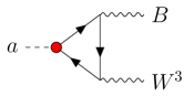
Figure 8: Illustration of fermionic one-loop contributions which induce an effective coupling $a\,B^{\mu\nu}\tilde{W}^{3}_{\mu\nu}$.

Gauge invariant ancestors of radiatively corrected couplings

As stated above, the operators $aB_{\mu\nu}\tilde{W}^{3\mu\nu}$ and $aW^{3}_{\mu\nu}\tilde{W}^{3\mu\nu}$ are neither custodial nor $SU(2)_{L}$ invariant. Nevertheless, there must be a fully gauge-invariant formulation of any possible correction to the effective Lagrangian and its corrections, because electroweak gauge symmetry is unbroken in nature. Indeed, in generic EFTs, one-loop corrections are expected to give contributions to higher order terms in the EFT expansion. Both in the SMEFT and in the linear ALP EFT, these contributions are always finite, i.e. all UV-divergences are reabsorbed order-by-order in the EFT expansion. Well-known examples in the SM are the magnetic and electric dipole moments in the SM, whose gauge invariant version corresponds to operators with mass dimension six and above.

Higher order radiative corrections, and in particular mass dependent ones (which are equivalent to multiple Higgs insertions that then take a vev) can imply that a full tower of operators may be needed to formulate those corrections in a gauge invariant way. The putative $SU(2)_{L}\times U(1)_{Y}$-invariant ancestors of the four gauge anomalous couplings in the Lagrangian $\mathcal{L}_{a}^{\text{total}}+\mathcal{\delta L}_{a}^{\text{total}}$, i.e. Eqs. (5) and Eq. (114), can be formulated alike to those in Ref. Helset:2020yio for CP-conserving Higgs couplings. For our ALP set, we expect $v$-dependent radiative corrections encoded in the gauge invariant operators

$$(5+2n):\quad a\,(\Phi^{\dagger}\Phi)^{n}\,B^{\mu\nu}\tilde{B}_{\mu\nu}\,,$$ (116)

$$(5+2n):\quad a\,(\Phi^{\dagger}\Phi)^{n}\,W^{\mu\nu}\tilde{W}_{\mu\nu}\,,$$ (117)

$$(7+2n):\quad a\,(\Phi^{\dagger}\Phi)^{n}\,(\Phi^{\dagger}\vec{\sigma}\Phi)\,\vec{W}^{\mu\nu}\tilde{B}_{\mu\nu}\longrightarrow a\,B^{\mu\nu}\tilde{W}^{3}_{\mu\nu}\,,$$ (118)

$$(9+2n):\quad a\,(\Phi^{\dagger}\Phi)^{n}\,(\Phi^{\dagger}\vec{\sigma^{a}}\Phi)\,(\Phi^{\dagger}\vec{\sigma^{b}}\Phi)\,\vec{W}_{a}^{\mu\nu}\tilde{W}_{b\,\mu\nu}\longrightarrow a\,W_{3}^{\mu\nu}\tilde{W}^{3}_{\mu\nu}\,,$$ (119)

where $n$ is integer, $n\geq 0$. In the last two lines it is indicated that those two towers of operators lead –after spontaneously symmetry breaking– to the custodial and $SU(2)_{L}$ non-invariant couplings $a\,B^{\mu\nu}\tilde{W}^{3}_{\mu\nu}$ and $a\,W_{3}^{\mu\nu}\tilde{W}^{3}_{\mu\nu}$ postulated earlier: note that their mass dimension is at least seven and nine, respectively, and that they vanish for $v=0$. In contrast, the couplings in the first two lines can receive mass-independent one-loop corrections even for $n=0$, as computed in the previous section. An important consequence of this is that loops induced by dimension-5 ALP operators can give UV-divergent contributions to the structures in (116) and (117) for $n=0$, while contributions to all other structures must be finite. We find that this is indeed the case for $\Delta_{WW}$ and $\Delta_{BW}$.

A pertinent question is the scale that would weight down those higher-dimension operators. Only one inverse power of $f_{a}$ is possible, because ALP insertions must enter as powers of $a/f_{a}$, and only one ALP insertion is considered here. The remaining scale dependence must then correspond to either another BSM scale (not considered here) or simply to SM mass parameters when only SM radiative corrections are present as in the present work, i.e. to powers of the electroweak scale. These SM corrections should generate coefficient contributions proportional in addition to the SM sources of custodial breaking.

5.1 Gauge invariance relations among effective electroweak couplings at one-loop

It is easy to verify that $\Delta_{WW}=\Delta_{BW}=0$ in the massless limit, i.e. for $v=0$, and the one-loop corrections to the anomalous gauge couplings satisfy the tree-level gauge invariance relations Eq. (36). Instead, when mass corrections are taken into account, non-zero values for $\Delta_{WW}$ and $\Delta_{BW}$ do emerge. As an example, our results show that the contributions stemming from ALP-fermion coupling insertions –see Fig. 8– are finite and take the general form

$$\Delta_{BW} =Y_{L}\,(F_{L}(m_{1})-F_{L}(m_{2}))+Y_{R1}\,F_{R}(m_{1})-Y_{R2}\,F_{R}(m_{2})\,,$$ (120)

where $m_{i=1,2}$ denote fermion masses of $SU(2)_{L}$ fermion partners and the functions $F_{R}(m)$ and $F_{L}(m)$ cancel in the massless fermion limit, $F_{L,R}(0)=0$. In other words, a non-vanishing $\Delta_{BW}$ coupling requires as expected that the sources of custodial breaking be at play: different fermion hypercharges and non-degenerate fermion partners running in the loop.

More in general, it follows from the analysis above that the tree-level gauge invariance relations in Eq. (36) are to be substituted by the one-loop corrected ones, which we choose to parametrize as:

$$g^{\text{eff}}_{aWW}=g^{\text{eff}}_{a\gamma\gamma}+\frac{\bar{c}_{w}}{2\bar{s}_{w}}g^{\text{eff}}_{a\gamma Z}-\frac{\bar{c}_{w}}{2\bar{s}_{w}}\Delta_{BW}-\Delta_{WW}\,,$$ (121)

$$g^{\text{eff}}_{aZZ}=g^{\text{eff}}_{a\gamma\gamma}+\frac{\bar{c}_{w}^{2}-\bar{s}_{w}^{2}}{2\bar{c}_{w}\bar{s}_{w}}g^{\text{eff}}_{a\gamma Z}-\frac{1}{2\bar{c}_{w}\bar{s}_{w}}\Delta_{BW}\,,$$

where ${\bar{c}_{w}}$ was defined in Eq. (51). These one-loop corrections gauge invariance relations may impact on the limits inferred for a given coupling from the experimental bounds on another couplings known at present with higher precision (e.g. the bounds on the ALP-$ZZ$ anomalous coupling obtained from the experimental limits on the ALP-$\gamma\gamma$ coupling in certain mass regimes Bauer:2017ris ; Alonso-Alvarez:2018irt ; Gavela:2019wzg ).

Limit $m_{\text{f}}^{2},M_{Z}^{2},M_{W}^{2},M_{H}^{2}\ll p^{2}\leq m_{t}^{2}$

Because $\Delta_{WW}$ and $\Delta_{BW}$ vanish for $v=0$, they vanish in the limit $p^{2}\rightarrow\infty$. The contribution of the top quark may thus dominate for large $p^{2}$ close to $m_{t}^{2}$. That is, the contribution of the top-ALP coupling ${\bf{c}}_{t}$ may dominate in the limit in which all SM particle masses but the top one are neglected with respect to the ALP $p^{2}$:

$$\Delta_{BW}\sim-c_{t}\,\frac{\alpha_{em}}{\pi c_{w}s_{w}}\frac{m_{t}^{2}}{p^{2}}\Bigg{\{}6+6i\sqrt{1-\frac{4m_{t}^{2}}{p^{2}}}f\left(\frac{4m_{t}^{2}}{p^{2}}\right)-4f\left(\frac{4m_{t}^{2}}{p^{2}}\right)^{2}\Bigg{\}}\,,$$ (122)

$$\Delta_{WW}\sim c_{t}\,\frac{3\alpha_{em}}{2\pi s_{w}^{2}}\frac{m_{t}^{2}}{p^{2}}\Bigg{\{}1+m_{t}^{2}\mathcal{C}\left(0,0,p^{2},m_{t},0,m_{t}\right)\Bigg{\}}\,,$$ (123)

where the function $f(\tau)$ was defined in Eq. (57) and $\mathcal{C}$ is defined in Eqs. (LABEL:functionC)-(173) of App. C.2. Notice that these expressions vanish in the limit $p^{2}\rightarrow\infty$, as they must.

6 Some phenomenological consequences of loop-induced ALP couplings

High-precision measurements may be increasingly able to probe loop corrections to tree-level effective couplings. Currently, sensitivity to loop-induced couplings is particularly interesting when a tree-level coupling is suppressed and the loop contributions dominate.

In this section we are going to explore two examples of such situations: high-energy gluon-initiated production of an electroweak ALP, and very precise low-energy searches for ALPs which rely on couplings to electron-positron. In both cases, we focus on the loop effects of the ALP coupling to top quarks.

6.1 LHC probes for heavy ALPs

Figure 9: One-loop contribution to ALP production via gluon-fusion, and its decay to a pair of tops.

In the Lagrangian Eq. (5), we provided the ALP with couplings to the whole SM: the electroweak bosons, gluons and fermions. This is a rather general coupling structure, yet ALPs may have restrictions on how they communicate at tree-level to the SM. For example, ALPs could originate from a UV sector participating in the mechanism of electroweak symmetry breaking, coupled to the $SU(2)_{L}\times U(1)_{Y}$ sector and not to the $SU(3)_{c}$ one, e.g. in Composite Higgs models where an additional heavy CP-odd state arises as a partner to the Composite Higgs No:2015bsn ; Croon:2015naa . This is just an example of theories with vanishing or very suppressed tree-level effective ALP-gluon coupling ($g_{agg}$ in Eq. (63)): an electroweak ALP.

These models of electroweak ALPs would be hard to probe at the LHC, as protons are mainly made of light quarks and gluons. Then, the leading contribution to gluon-fusion cross-section could correspond to integrating out tops. For definiteness, let us consider exclusively the ALP-top diagonal coupling $c_{t}$ defined in Eq. (39),

$$\mathscr{L}\supset c_{t}\,\dfrac{\partial_{\mu}a}{2f_{a}}\,\left(\bar{t}\gamma^{\mu}\gamma_{5}t\right)\,.$$ (124)

The ALP production would then be mediated by a top running in the gluon loop and could be constrained, for instance, in $gg\rightarrow a\rightarrow t\bar{t}$ processes, as illustrated in Fig. 9. In this process, the ALP could be either resonant or non-resonant Gavela:2019cmq , depending on its mass.

For definiteness, here we consider ALPs with $m_{a}>2m_{t}$, such that the top-antitop pair can be resonant. This allows us to derive constraints from existing searches for resonances in $t\bar{t}$ final states, that are at a very mature stage in the LHC collaborations. This is true in particular at high-mass, where the fully hadronic topology can be accessed using jet substructure techniques. As an illustration of how LHC probes could be used to search for heavy ALPs, we re-interpret the recent ATLAS analysis ATLAS:2020lks to set bounds on $c_{t}/f_{a}$.

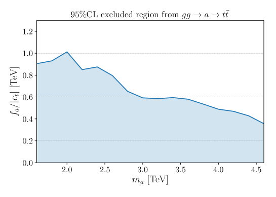
Figure 10: Limits on $f_{a}/|c_{t}|$, as a function of the ALP mass, extracted from the all-hadronic $t\bar{t}$ resonance search by ATLAS of Ref. ATLAS:2020lks .

We simulate separately the pure $gg\rightarrow a\rightarrow t\bar{t}$ signal and the component stemming from the interference of this process with SM $gg\rightarrow t\bar{t}$ production. Expressing $g_{agg}^{\text{eff}}$ as a function of $c_{t}$ as in Eq. (63), the former scales with $(c_{t}/f_{a})^{4}$ and the latter with $(c_{t}/f_{a})^{2}$. The simulation is performed generating $10^{5}$ events in each channel with MadGraph5_aMC@NLO Alwall:2011uj , using an in-house UFO implementation of the Lagrangian in Eq. (5). Variations of $g_{agg}^{\text{eff}}$ with $p^{2}$ are neglected, as they only induce a few % correction to the numerical value of the gluon coupling. The imaginary part stemming from expanding the $B_{1}$ loop function is also subdominant and can be safely neglected in the simulation.

We perform a very simple analysis at parton level, without decaying the top quarks and without performing full parton shower and detector simulations. To partially compensate for this, a gaussian smearing with a $6\%$ width is applied to the simulated top-antitop invariant mass ($m_{t\bar{t}}$) distribution, and the latter is multiplied by a $m_{t\bar{t}}$-dependent suppression factor estimated from Fig. 2 in Ref. ATLAS:2020lks , that accounts for the tagging efficiencies. The acceptance correction is implemented by applying, at the generator level, the cuts reported in Ref. ATLAS:2020lks on the top quarks pseudo-rapidities $\eta_{t,\bar{t}}$ and transverse momenta $p_{T}(t,\bar{t})$, and on their rapidity and azimuthal-angle separations, $\Delta y_{t\bar{t}}$ and $\Delta\phi_{t\bar{t}}$ respectively.

The distribution obtained (summing signal and interference components) is compared to the difference between measured and predicted number of events in the $m_{t\bar{t}}$ spectra reported in Ref. ATLAS:2020lks , that is available on HEPdata. We implement a basic test statistics constructing a $\chi^{2}$ as

$$\chi^{2}(c_{t}/f_{a})=\sum_{k}\frac{1}{\sigma_{k}^{2}}\left[\frac{c_{t}^{4}}{f_{a}^{4}}\,a_{k}+\frac{c_{t}^{2}}{f_{a}^{2}}\,i_{k}+b_{k}-d_{k}\right]\,,$$ (125)

where the index $k$ runs over the bins of the $m_{t\bar{t}}$ distributions for the 1- and 2-$b$-tagged signal regions, $a_{k}$ ($i_{k}$) is the number of events estimated for the pure ALP signal (ALP-SM interference) in the $k$-th bin with $c_{t}/f_{a}=1\,\mathrm{TeV^{-1}}$. In this equation, $b_{k}$ ($d_{k}$) is the number of expected background events (observed events) reported by the ATLAS Collaboration. Finally, the uncertainty $\sigma_{k}$ is estimated by summing in quadrature the total systematic uncertainty reported by ATLAS, the statistical error $\sqrt{d_{k}}$ on the measured data points and the statistical uncertainty associated to our Monte Carlo simulation. As a conservative choice, bins with 0 observed events are removed from the analysis, as in this case a $\chi^{2}$ statistics cannot be applied. We repeat this analysis for various values of $m_{a}$ in the range from $1.6$ to $4.6\,\mathrm{TeV}$ and extract, for each value, a 95%CL upper limit on $c_{t}/f_{a}$.

The results of this naive re-interpretation are shown in Fig. 10. The limits on $f_{a}$ obtained lie at the boundaries of a good effective description of the ALP Lagrangian as, for $|c_{t}|=1$, the bound on $f_{a}$ is mostly below $m_{a}$. On the other hand, in a strongly interacting regime where $|c_{t}|\simeq 4\pi$ (as could be the case of a Composite Higgs model), the limits on $f_{a}$ improve by an order of magnitude and result well above $m_{a}$. A dedicated analysis, potentially extended to the leptonic and semi-leptonic channels, could improve these bounds significantly.

6.2 Limits on the couplings to top quarks for light ALPs

Another interesting use of loop-induced ALP couplings appears when a tree-level coupling is very well measured and can provide a good constraint on loop-induced couplings, assuming no substantial cancellations happen between tree and loop-induced couplings. Among these, the loop-induced ALP-electron diagonal coupling $c_{e}$ (defined in Eq. (41)),

$$\mathscr{L}\supset c_{e}\,\dfrac{\partial_{\mu}a}{2f_{a}}\,\left(\bar{e}\gamma^{\mu}\gamma_{5}e\right)\,,$$ (126)

is particularly interesting as electrons are found in stable matter. Astrophysical objects like red giants or precise non-collider experiments such as Dark Matter Direct Detection experiments provide an excellent handle on that coupling. Here we consider the current limits on the axion-electron coupling collected in Ref. ciaran_o_hare_2020_3932430 , that include results from Red Giants Capozzi:2020cbu , Solar neutrinos Gondolo:2008dd and LUX LUX:2017glr , which are derived for solar axions and extend to very low ALP masses, as well as from Edelweiss EDELWEISS:2018tde , PandaX PandaX:2017ock , SuperCDMS SuperCDMS:2019jxx and XENON-1T XENON:2019gfn ; XENON:2020rca ; VanTilburg:2020jvl , that cover the region $100\,\mathrm{eV}\lesssim m_{a}\lesssim 100\,\mathrm{keV}$ assuming the ALP to be the main DM constituent. The most stringent bounds are those from red giants and from DM direct detection at XENON-1T, and give $|c_{e}^{\text{eff}}|\,(m_{e}/f_{a})\lesssim 10^{-13}$.

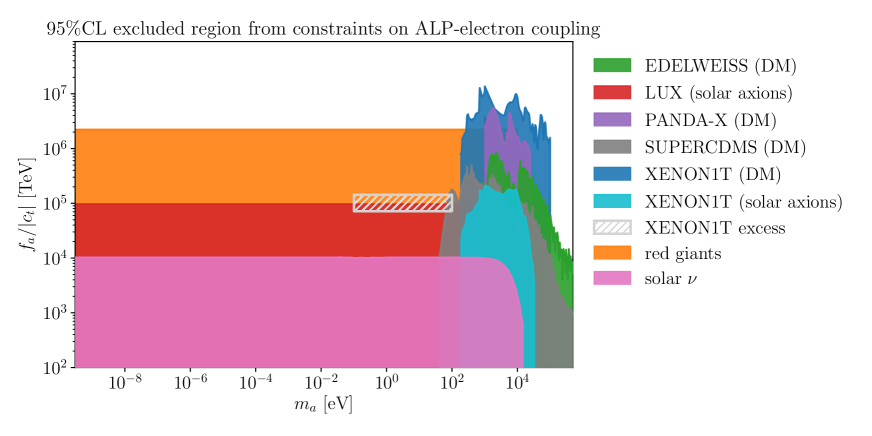
Figure 11: Limits on $f_{a}/|c_{t}|$ as a function of the ALP mass, extracted rescaling existing constraints on the ALP-electron coupling, taken from Ref. ciaran_o_hare_2020_3932430 . The grey hatched box marks the region roughly compatible with the excess observed by XENON1T XENON:2020rca .

These limits can be translated into limits on the diagonal ALP-top coupling, using the one-loop contributions computed in Sec. 4.6, corresponding to diagram E in Fig. 6, see also Refs. Feng:1997tn ; Arias-Aragon:2020shv . Note that in DM direct detection experiments the typical energy range is the keV, hence our expressions must be taken in the limit of low-momentum exchange in the detector between the ALP and the electron, i.e. below the electron mass. In this case one finds the log-enhanced expression found in Eq. (111), namely:

$$c_{e}^{\text{eff}}\simeq 2.48\,c_{t}\,\alpha_{em}\,\log\left(\frac{\Lambda^{2}}{m_{t}^{2}}\right)\,.$$ (127)

For consistency, the cutoff of the loop integrals $\Lambda$ should be of the same order as $f_{a}$. As the $\Lambda$ dependence is logarithmic we will use $\Lambda=10^{6}\,\mathrm{TeV}$ in this equation, to extract the bounds on $f_{a}/c_{t}$ shown in Fig. 11, from which it follows

$$f_{a}/|c_{t}|>2.2\times 10^{6}\,\mathrm{TeV}$$ (128)

in the entire range considered. If the ALP is assumed to be DM, XENON1T bounds apply, leading to the stronger constraint

$$f_{a}/|c_{t}|>1.4\times 10^{7}\,\mathrm{TeV}\,.$$ (129)

XENON1T recently observed an excess in their data, which could have been explained by solar axions coupled to electrons and/or photons in the mass range $m_{a}\sim 0.1-100$ eV for the QCD axion XENON:2020rca ; Gao:2020wer . Thus, instead of a limit, in this case XENON1T would identify a finite preferred region in the plane $(g_{a\gamma\gamma},c_{e}/f_{a})$. Unfortunately, this interpretation of a QCD axion is in conflict with the data from red giants. Nevertheless and for the sake of the exercise, one can consider what would be the preferred value for $f_{a}/c_{t}$ if that XENON1T excess was taken at face value. Using then Eq. (127), and the one-loop corrections to $g_{a\gamma\gamma}$ computed in Sec. 4.1 which correspond to diagram C in Fig. 4, it follows that the induced value of $g_{a\gamma\gamma}$ is strongly suppressed for the ALP mass range considered here ($p^{2}=m_{a}^{2}\ll m_{t}^{2}$): $g_{a\gamma\gamma}^{\text{eff}}\lesssim 10^{-8}\alpha_{em}c_{t}/f_{a}\ll c_{e}^{\text{eff}}/f_{a}$. In this limit, the results from XENON1T could be interpreted as a preferred range for $c_{e}^{\text{eff}}$ independent of $g_{a\gamma\gamma}$. This broadly includes values $2\times 10^{-12}\lesssim|c_{e}^{\text{eff}}|(m_{e}/f_{a})\lesssim 4\times 10^{-12}$. The projection of this interval in terms of $f_{a}/c_{t}$ is shown as a grey-hatched region in Fig. 11.

Finally, note that the type of analysis carried out in this subsection can be also applied to the flavour-diagonal ALP-bottom coupling $c_{b}$ (defined in Eq. (40)). Numerically, limits on $f_{a}/c_{b}$ can be approximately estimated rescaling by $m_{b}^{2}/m_{t}^{2}$ Arias-Aragon:2020shv those on $f_{a}/c_{t}$ in Eqs. (128) and (129) above, leading respectively to $f_{a}/|c_{b}|>1.0\times 10^{3}\,\mathrm{TeV}$ and $f_{a}/|c_{b}|>6.5\times 10^{3}\,\mathrm{TeV}$, for $\Lambda=10^{3}\,\mathrm{TeV}$.

7 Conclusions

The search for axions and ALPs is intensifying in both the energy and the precision frontiers. The vastly different energy regions explored range from those typical of astrophysics and low-energy laboratory experiments to collider energies. At the same time, increasingly precise probes are targeted e.g. photon and/or invisible channels in rare hadron decays and other low-energy channels. The point is well past in which the estimation of one-loop effects in the couplings of ALPs to SM particles is needed to explore optimally BSM physics through the detection of pseudo-Goldstone bosons signals. From the theoretical point of view, effective Lagrangian formulations allow to pursue this quest in a very model-independent way.

In this work, we have first clarified the relations among alternative –complete and non-redundant– CP-even bases for the $d=5$ ALP linear effective Lagrangian. In doing so, we derived the exact relations between bases which differ in their choices of fermionic operators constructed with left-handed and right-handed currents and/or chirality-flip couplings. We identified the precise combinations of gauge anomalous couplings involved in trading different bases. This includes the relations stemming from the anomalous global $B+L$ current and the conserved $B-L$ one. Although we then chose to work on a complete and non-redundant basis containing gauge anomalous operators plus all possible right-handed fermionic currents and certain couplings made out of left-handed currents, the relations obtained will allow easy translation of the results to other bases.

Furthermore, illustrative practical checks of bases equivalences were as well performed. For instance, the purely bosonic operator $\mathbf{O}_{a\Phi}$ can be written either as a combination of right-handed fermion currents or as a combination of left-handed fermion currents, right-handed ones and gauge anomalous couplings: it is explicitly shown how all anomalous corrections vanish at one-loop level, as they should.

In a second step, we have computed the complete one-loop corrections –thus including all divergent and finite terms– to all possible CP-even couplings of an ALP to SM fields, for a generic off-shell ALP and on-shell SM particles. Our results are formulated in the form of the effective one-loop interactions $\{g^{\text{eff}}_{agg}\,,g^{\text{eff}}_{a\gamma\gamma},\,g^{\text{eff}}_{aWW},\,g^{\text{eff}}_{aZZ}\,,g^{\text{eff}}_{a\gamma Z}\,,c_{\text{f}}^{\text{eff}}\}$, where the latter is computed for all SM fermions –light and heavy– but restricted to flavour diagonal external channels. Moreover three-generation CKM mixing is disregarded in the loop corrections. Neutrino masses are disregarded as well. Our computations thus carry to novel territory previous studies restricted to on-shell ALPs and to certain channels and limits. All our computations have been performed in the covariant $R_{\xi}$ gauge, and the intermediate $\xi$-dependent steps made publicly available at NotebookArchive, together with the exact final gauge-invariant results. The latter are shown as well in App. C, while in the main text limits relevant for high, intermediate and low energy experiments are extracted. Particular attention has been dedicated to the isolation of infrared divergences when present. As a byproduct, the UV divergent terms of our computations also allowed to do a straightforward check of recent RG results in the literature in different bases.

An illustration of the reach of our results is the impact that any putative ALP coupling induces at one-loop on any other ALP interaction. For instance, we explored how, for heavy ALPs, the ALP-top coupling can be constrained by LHC measurements of top-pair final states, processes which are induced at one-loop by this coupling. These channels, pumped up by gluon fusion via a top loop, open up the possibility of studying many ALP final states with a sizeable cross-section, even when the tree-level coupling ALP-gluon would be zero. We also explored constraints on ALP-top interactions for light ALPs. In this case, the strictest limits are those derived from bounds on the ALP-electron coupling, extracted from astrophysical constraints and from DM Direct Detection searches Feng:1997tn .

An interesting point also clarified in this work is the one-loop modification of the electroweak tree-level gauge invariance relations. These are relevant as far as custodial symmetry breaking, i.e. mass and hypercharge differences, are relevant. We have determined these corrections, which will impact future one-loop extractions at LHC and other experiments of the sensitivity to a given ALP coupling from more precise data on another ALP coupling (e.g. $g_{aWW}$ from data on $g^{\text{eff}}_{a\gamma\gamma}$ or $g^{\text{eff}}_{a\gamma Z}$, and similar analyses).

A plethora of experimental channels should be explored using the results of this paper. Future directions include the one-loop complete results with all external particles off-shell and also flavour non-diagonal channels. A related interesting task is the computation of box and other diagrams for certain physical processes, which is mandatory to cancel all infrared divergences in processes involving $g_{agg}$, $g_{aWW}$ and $c_{\text{f}}^{\text{eff}}$. Finally, the analysis of the ALP bases should be extended to include CP violation in the ALP couplings. These and other exciting developments lie ahead in the BSM path to uncover novel pseudo-Goldstone boson physics.

Appendix A Standard Model equations of motion

In this Appendix we report the SM EOM for the fermion and Higgs fields, that are relevant for the discussion in Sect. 2 and App. B. For chiral fermions, the EOM read

$$i\not{D}Q_{L} =\Phi Y_{d}d_{R}+\tilde{\Phi}Y_{u}u_{R}\,, i\not{D}u_{R} =\tilde{\Phi}^{\dagger}Y_{u}^{\dagger}Q_{L}\,, i\not{D}d_{R} =\Phi^{\dagger}Y_{d}^{\dagger}Q_{L}\,,$$ (130)

$$i\not{D}L_{L} =\Phi Y_{e}e_{R}\,, i\not{D}e_{R} =\Phi^{\dagger}Y_{e}^{\dagger}L_{L}\,,$$ (131)

where flavor index contractions are implicit. For the conjugate fields they imply

$$-i\bar{Q}_{L}\overleftarrow{\not{D}} =\bar{d}_{R}Y_{d}^{\dagger}\Phi^{\dagger}+\bar{u}_{R}Y_{u}^{\dagger}\tilde{\Phi}^{\dagger}\,, -i\bar{u}_{R}\overleftarrow{\not{D}} =\bar{Q}_{L}Y_{u}\tilde{\Phi}\,, -i\bar{d}_{R}\overleftarrow{\not{D}} =\bar{Q}_{L}Y_{d}\Phi\,,$$ (132)

$$-i\bar{L}_{L}\overleftarrow{\not{D}} =\bar{e}_{R}Y_{e}^{\dagger}\Phi^{\dagger}\,, -i\bar{e}_{R}\overleftarrow{\not{D}} =\bar{L}_{L}Y_{e}\Phi\,.$$ (133)

The EOM for the Higgs field reads

$$\square\Phi_{i} =-\left[\bar{d}_{R}Y_{d}^{\dagger}(Q_{L})_{i}+(\bar{Q}_{L}i\sigma^{2})_{i}Y_{u}u_{R}+\bar{e}_{R}Y_{e}^{\dagger}(L_{L})_{i}\right]+\frac{m_{h}^{2}}{2}\Phi_{i}-2\lambda(\Phi^{\dagger}\Phi)\Phi_{i}\,,$$ (134)

$$\square\Phi^{\dagger}_{i} =-\left[(\bar{Q}_{L})_{i}Y_{d}d_{R}+\bar{u}_{R}Y_{u}^{\dagger}(i\sigma^{2}Q_{L})_{i}+(\bar{L}_{L})_{i}Y_{e}e_{R}\right]+\frac{m_{h}^{2}}{2}\Phi^{\dagger}_{i}-2\lambda(\Phi^{\dagger}\Phi)\Phi^{\dagger}_{i}\,,$$ (135)

where $i$ is a free $SU(2)_{L}$ index and we have taken $V(\Phi^{\dagger}\Phi)=-(m_{H}^{2}/2)\Phi^{\dagger}\Phi+\lambda(\Phi^{\dagger}\Phi)^{2}$, where $m_{H}$ and $\lambda$ denote respectively the Higgs mass and self-coupling.

The use of fermion EOM is tantamount to chiral rotations of fermion fields, at the classical level. When considering loop effects as in this work, they must be supplemented by the contributions of the SM anomalous global currents, i.e.

$$\partial_{\mu}(\bar{Q}_{L}^{i}\gamma^{\mu}Q_{L}^{i}) \supset\dfrac{g^{\prime 2}}{96\pi^{2}}B_{\mu\nu}\tilde{B}^{\mu\nu}+\dfrac{3g^{2}}{32\pi^{2}}W_{\mu\nu}^{\alpha}\tilde{W}^{\alpha\mu\nu}+\dfrac{g_{s}^{2}}{16\pi^{2}}G_{\mu\nu}^{a}\tilde{G}^{a\mu\nu}\,,$$ (136)

$$\partial_{\mu}(\bar{u}_{R}^{i}\gamma^{\mu}u_{R}^{i}) \supset-\dfrac{g^{\prime 2}}{12\pi^{2}}B_{\mu\nu}\tilde{B}^{\mu\nu}-\dfrac{g_{s}^{2}}{32\pi^{2}}G_{\mu\nu}^{a}\tilde{G}^{a\mu\nu}\,,$$ (137)

$$\partial_{\mu}(\bar{d}_{R}^{i}\gamma^{\mu}d_{R}^{i}) \supset-\dfrac{g^{\prime 2}}{48\pi^{2}}B_{\mu\nu}\tilde{B}^{\mu\nu}-\dfrac{g_{s}^{2}}{32\pi^{2}}G_{\mu\nu}^{a}\tilde{G}^{a\mu\nu}\,,$$ (138)

$$\partial_{\mu}(\bar{L}_{L}^{i}\gamma^{\mu}L_{L}^{i}) \supset\dfrac{g^{\prime 2}}{32\pi^{2}}B_{\mu\nu}\tilde{B}^{\mu\nu}+\dfrac{g^{2}}{32\pi^{2}}W_{\mu\nu}^{\alpha}\tilde{W}^{\alpha\mu\nu}\,,$$ (139)

$$\partial_{\mu}(\bar{e}_{R}^{i}\gamma^{\mu}e_{R}^{i}) \supset-\dfrac{g^{\prime 2}}{16\pi^{2}}B_{\mu\nu}\tilde{B}^{\mu\nu}\,,$$ (140)

where we are not summing over the index $i$.

Appendix B Field redefinitions and operator basis reduction

In this appendix we consider the ALP-dependent field redefinitions that are required in order to relate and reduce the operator basis:

$$\Phi \mapsto\exp\left[ix_{\Phi}\frac{a}{f_{a}}\right]\Phi\,, \mapsto\exp\left[i\mathbf{x}_{\text{f}}\frac{a}{f_{a}}\right]\text{f}\,,$$ f (141)

where in flavour space $\text{f}=\{Q_{L},u_{R},d_{R},L_{L},e_{R}\}$ are vectors and $\mathbf{x}_{\text{f}}=\mathbf{x}_{\text{f}}^{ij}$ are tensors. For notation simplicity, the subindices $\{L,R\}$ will be omitted, i.e. $\text{f}=\{Q_{L},u_{R},d_{R},L_{L},e_{R}\}\equiv\{Q,u_{,}d_{,}L,e\}$. We take all rotation parameters $x_{\Phi}$ and $\mathbf{x}_{\text{f}}$ to be real, consistent with the assumption of CP conservation of the ALP couplings (the only CP-violation present is that of the SM contained in CKM, i.e. in the Yukawa matrices). Moreover, due to the hermicity of the Lagrangian it is only the symmetric component of the matrices $\mathbf{x}_{\text{f}}$ that contributes to a variation in it. Then, from now on we assume $\mathbf{x}_{\text{f}}$ to be symmetric, i.e. $\mathbf{x}_{\text{f}}^{ij}=\mathbf{x}_{\text{f}}^{ji}$, so $(\mathbf{x}_{\text{f}}+\mathbf{x}_{\text{f}}^{T})/2=\mathbf{x}_{\text{f}}$. Discussing the basis reduction in terms of field redefinitions rather than via the direct use of EOMs makes their impact on the $\mathbf{O}_{\tilde{X}}$ operators more transparent: because the fermion rotations are chiral, contributions to the latter are generated through the axial anomaly.

The general procedure for reducing the operator basis is as follows. The rotations in (141) are first applied to $\mathscr{L}_{SM}$ (Eq. (2)), and an expansion at $O(1/f_{a})$ is performed next. The net shift resulting from the most general rotation reads Brivio:2017ije

$$\Delta\mathscr{L}_{SM} =-x_{\Phi}\,\mathbf{O}_{a\Phi}-\sum_{\text{f}=Q,u,d,L,e}\mathbf{x}_{\text{f}}\mathbf{O}_{\text{f}}+\Big{[}\left(\mathbf{x}_{L}Y_{e}-Y_{e}\mathbf{x}_{e}-x_{\Phi}Y_{e}\right)\mathbf{O}_{e\Phi}$$ (142)

$$+\left(\mathbf{x}_{Q}Y_{d}-Y_{d}\mathbf{x}_{d}-x_{\Phi}Y_{d}\right)\mathbf{O}_{d\Phi}+\left(\mathbf{x}_{Q}Y_{u}-Y_{u}\mathbf{x}_{u}+x_{\Phi}Y_{u}\right)\mathbf{O}_{u\Phi}+\text{h.c.}\Big{]}$$

$$+\frac{g^{\prime 2}}{32\pi^{2}}\mathbf{O}_{\tilde{B}}\operatorname{Tr}\left[\frac{1}{3}\mathbf{x}_{Q}-\frac{8}{3}\mathbf{x}_{u}-\frac{2}{3}\mathbf{x}_{d}+\mathbf{x}_{L}-2\mathbf{x}_{e}\right]+\frac{g^{2}}{32\pi^{2}}\mathbf{O}_{\tilde{W}}\operatorname{Tr}\left[3\mathbf{x}_{Q}+\mathbf{x}_{L}\right]$$

$$+\frac{g^{2}_{s}}{32\pi^{2}}\mathbf{O}_{\tilde{G}}\operatorname{Tr}\left[2\mathbf{x}_{Q}-\mathbf{x}_{u}-\mathbf{x}_{d}\right]\,,$$

where the anomalous operators $\mathbf{O}_{\tilde{X}}$ are defined in Table 1, $\mathbf{O}_{\text{f}}$ are the chirality-conserving fermionic operators defined in Eqs (3) (4), $\mathbf{O}_{\text{f}\Phi}$ are the chirality-flip ones defined in Eq. (19), and finally $\mathbf{O}_{a\Phi}$ is defined in Table 2. The trace in the last two lines of Eq. (142) is over flavor indices, while in the first two lines the implicit contraction of flavour index of the effective coefficients and operators respects the convention in Eq. (6), e.g.

$$\left(\mathbf{x}_{L}Y_{e}-Y_{e}\mathbf{x}_{e}-x_{\Phi}Y_{e}\right)\mathbf{O}_{e\Phi}=\sum_{i,j}\left(\mathbf{x}_{L}Y_{e}-Y_{e}\mathbf{x}_{e}-x_{\Phi}Y_{e}\right)_{ij}\mathbf{O}^{ij}_{e\Phi}\,,\quad\text{etc.}\,,$$

while the expressions inside parenthesis are matrix products, i.e. $(\mathbf{x}_{L}Y_{e})_{ij}=\sum_{k}(\mathbf{x}_{L})_{ik}(Y_{e})_{kj}$.

At this point, one is free for instance to choose $x_{\Phi}$ and $\mathbf{x}_{\text{f}}$ so that the terms in $\Delta\mathscr{L}_{SM}$ cancel off against redundant operators in $\mathscr{L}_{a}^{\rm total}$. Or to choose values for combination of indices so as to remove one or all of the anomalous coefficients $c_{\tilde{X}}$. It is not hard to verify that each field transformation is equivalent –up to shifts to the anomalous bosonic operators– to the application of the EOM of the corresponding field, provided in App. A. In what follows, some specific applications of Eq. (142) are developed.

B.1 Relation between $\mathbf{O}_{a\Phi}$ and fermionic operators

Eq. (142) indicates that in order to remove $\mathbf{O}_{a\Phi}$ one needs to fix $x_{\Phi}=c_{a\Phi}$. This $\Phi$ rotation comes at the price of introducing a set of chirality-flip operators Georgi:1986df ; Gavela:2014vra ; Brivio:2017ije , i.e.

$$\mathbf{O}_{a\Phi}=Y_{u}\mathbf{O}_{u\Phi}-Y_{d}\mathbf{O}_{d\Phi}-Y_{e}\mathbf{O}_{e\Phi}+\text{h.c.}\,.$$ (143)

As $\mathbf{O}_{a\Phi}$ is a purely bosonic operator, the flavor structure of the fermionic operators in this equation necessarily reflects the SM flavour structure. In other words, it follows the MFV ansatz Chivukula:1987py ; Hall:1990ac ; D'Ambrosio:2002ex , where a $U(3)^{5}$ global flavor symmetry is present in the Lagrangian but for the Yukawa couplings, which are treated as spurions.

The combination of chirality-flip operators obtained can be traded next for chirality-preserving ones (plus in some cases shifts in the $\mathbf{O}_{\tilde{X}}$ operator coefficients) by fixing the quantities $\mathbf{x}_{\text{f}}$ such that the coefficients of $\mathbf{O}_{e\Phi},\mathbf{O}_{u\Phi},\mathbf{O}_{d\Phi}$ in Eq. (142) cancel. This is equivalent to applying the transformations of the fermion fields in Eqs. (145)–(150) below. For instance, it is possible to map $\mathbf{O}_{a\Phi}$ onto just 3 operators out of the whole set $\{\mathbf{O}_{u},\mathbf{O}_{d},\mathbf{O}_{e},\mathbf{O}_{Q},\mathbf{O}_{L}\}$, plus $\mathbf{O}_{\tilde{X}}$ operators. For example, the mapping onto the set $\{\mathbf{O}_{u},\mathbf{O}_{d},\mathbf{O}_{e}\}$ is achived choosing $\mathbf{x}_{e}^{ij}=\mathbf{x}_{d}^{ij}=-\mathbf{x}_{u}^{ij}=\delta^{ij}\,c_{a\Phi}$, and leads to Eq. (27), that is a combination of only right-handed fermionic currents. As it can be easily checked from Eq. (142), the contributions to gauge anomalous operators $\mathbf{O}_{\tilde{X}}$ cancel exactly in this case, which does not necessarily generalize to other choices.

For instance, one could alternatively map onto the set $\{\mathbf{O}_{Q},\mathbf{O}_{u},\mathbf{O}_{L}\}$ by choosing $\mathbf{x}_{L}^{ij}=\mathbf{x}_{Q}^{ij}=\mathbf{x}_{u}^{ij}/2=\delta^{ij}\,c_{a\Phi}$, which leads to

$$\mathbf{O}_{a\Phi} =-\operatorname{Tr}\left(\mathbf{O}_{L}+\mathbf{O}_{Q}+2\mathbf{O}_{u}\right)+\frac{1}{8\pi^{2}}\left(g^{2}\mathbf{O}_{\tilde{W}}-g^{\prime 2}\mathbf{O}_{\tilde{B}}\right)n_{g}\,.$$ (144)

This result does not mean that $\mathbf{O}_{a\Phi}$ is anomalous! In fact, we have explicitly checked that when the product $c_{a\Phi}\mathbf{O}_{a\Phi}$ is considered at $\mathcal{O}(\alpha)$, the contribution from the $\mathbf{O}_{\tilde{X}}$ terms on the last bracket are compensated exactly by the anomalous contributions stemming from the insertion in Fig. 4 diagram C of the operators in the first bracket ($\mathbf{O}_{u}$, $\mathbf{O}_{Q}$ and $\mathbf{O}_{L}$), and only $\mathcal{O}(m_{\text{f}}^{2})$ finite terms of remain from the loop contribution. When instead the same computation is performed using the expression for $\mathbf{O}_{a\Phi}$ in Eq. (27), i.e. as combination of the right-handed set $\{\mathbf{O}_{u},\mathbf{O}_{d},\mathbf{O}_{e}\}$, the anomalous contributions they induce cancel each other and only the same $\mathcal{O}(m_{\text{f}}^{2})$ terms are present, as they should.

B.2 Relations among fermionic operators

Collecting the terms proportional to $\mathbf{x}_{\text{f}}$ in Eq. (142) one can infer relations among the fermionic operators. Writing explicitly the flavor indices $i,j$, it follows that the relations between chirality preserving and chirality-flip operators (plus anomalous couplings) read fermion structures can be

$$\mathbf{O}_{Q}^{ij} =\left[\mathbf{O}_{d\Phi}^{ik}\,(Y_{d})_{jk}+\mathbf{O}_{u\Phi}^{ik}\,(Y_{u})_{jk}+(\mathbf{O}_{d\Phi}^{\dagger})^{kj}\,(Y_{d}^{\dagger})_{ki}+(\mathbf{O}_{u\Phi}^{\dagger})^{kj}\,(Y_{u}^{\dagger})_{ki}\right]$$ (145)

$$\,\,\,\,\,\,+\left[\frac{g^{\prime 2}}{96\pi^{2}}\mathbf{O}_{\tilde{B}}+\frac{3g^{2}}{32\pi^{2}}\mathbf{O}_{\tilde{W}}+\frac{g_{s}^{2}}{16\pi^{2}}\mathbf{O}_{\tilde{G}}\right]\,\delta^{ij}\,,$$ (146)

$$\mathbf{O}_{u}^{ij} =\left[-\mathbf{O}_{u\Phi}^{kj}\,(Y_{u})_{ki}-(\mathbf{O}_{u\Phi}^{\dagger})^{ik}\,(Y_{u}^{\dagger})_{jk}\right]-\left[\frac{g^{\prime 2}}{12\pi^{2}}\mathbf{O}_{\tilde{B}}+\frac{g_{s}^{2}}{32\pi^{2}}\mathbf{O}_{\tilde{G}}\right]\,\delta^{ij}\,,$$ (147)

$$\mathbf{O}_{d}^{ij} =\left[-\mathbf{O}_{d\Phi}^{kj}\,(Y_{d})_{ki}-(\mathbf{O}_{d\Phi}^{\dagger})^{ik}\,(Y_{d}^{\dagger})_{jk}\right]-\left[\frac{g^{\prime 2}}{48\pi^{2}}\mathbf{O}_{\tilde{B}}+\frac{g_{s}^{2}}{32\pi^{2}}\mathbf{O}_{\tilde{G}}\right]\,\delta^{ij}\,,$$ (148)

$$\mathbf{O}_{L}^{ij} =\left[\mathbf{O}_{e\Phi}^{ik}\,(Y_{e})_{jk}+(\mathbf{O}_{e\Phi}^{\dagger})^{kj}\,(Y_{e}^{\dagger})_{ki}\right]+\left[\frac{g^{\prime 2}}{32\pi^{2}}\mathbf{O}_{\tilde{B}}+\frac{g^{2}}{32\pi^{2}}\mathbf{O}_{\tilde{W}}\right]\,\delta^{ij}\,,$$ (149)

$$\mathbf{O}_{e}^{ij} =\left[-\mathbf{O}_{e\Phi}^{kj}\,(Y_{e})_{ki}-(\mathbf{O}_{e\Phi}^{\dagger})^{ik}\,(Y_{e}^{\dagger})_{jk}\right]-\frac{g^{\prime 2}}{16\pi^{2}}\mathbf{O}_{\tilde{B}}\,\delta^{ij}\,,$$ (150)

where a sum over $k$ is understood. Combining them, the relations between chirality-conserving operators and chirality-flip ones are determined.

The equations above showed how to express the chirality-conserving couplings as combinations of chirality-flip ones. What about the inverse relation? It is clear from the counting of degrees of freedom shown earlier that the latter cannot be achieved in all generality. Indeed, only very particular combinations – relatively weighed by Yukawa factors– of a given chirality-flip operator can be extracted from Eqs. (145)-(150), and written in terms of chirality-conserving plus anomalous couplings: this reduces in practice their $n_{g}^{2}$ degrees of freedom per fermionic operator (which sums to a total of $3n_{g}^{2}$ fermionic parameters in the ALP Lagrangian) to an active number of $n_{g}(5n_{g}+3)/2-1$ fermionic parameters in total.

B.3 Purely fermionic bases: removing anomalous operators

Finally, one could ask whether the anomalous operators $\mathbf{O}_{\tilde{X}}$ could be removed altogether from the basis, trading them for fermionic structures. In order to do this, one needs to impose

$$\frac{g^{\prime 2}}{32\pi^{2}}\operatorname{Tr}\left[\frac{1}{3}\mathbf{x}_{Q}-\frac{8}{3}\mathbf{x}_{u}-\frac{2}{3}\mathbf{x}_{d}+\mathbf{x}_{L}-2\mathbf{x}_{e}\right] =-c_{\tilde{B}}\,,$$ (151)

$$\frac{g^{2}}{32\pi^{2}}\operatorname{Tr}\left[3\mathbf{x}_{Q}+\mathbf{x}_{L}\right] =-c_{\tilde{W}}\,.$$ (152)

$$\frac{g_{s}^{2}}{32\pi^{2}}\operatorname{Tr}\left[2\mathbf{x}_{Q}-\mathbf{x}_{u}-\mathbf{x}_{d}\right] =-c_{\tilde{G}}\,.$$ (153)

It is not difficult to show explicitly that the anomalous bosonic operators cannot be completely replaced by purely chirality-conserving fermionic ones.  Indeed, it follows from Eq. (142) that the conditions to remove all chirality-flip terms are

$$\mathbf{x}_{Q}Y_{u}-Y_{u}\mathbf{x}_{u} =0\,,$$ (154)

$$\mathbf{x}_{Q}Y_{d}-Y_{d}\mathbf{x}_{d} =0\,,$$

$$\mathbf{x}_{L}Y_{e}-Y_{e}\mathbf{x}_{e} =0\,,$$

and it is not possible to satisfy simultaneously these equations and the conditions in Eqs. (151)–(153). Nevertheless, it is sufficient to relax two of the conditions in (154) in order for the system to be solvable. This implies that any solution of Eqs. (145)-(150) always involve chirality-flip terms. One example is:

$$\mathbf{O}_{\tilde{B}} =-\frac{16\pi^{2}}{g^{\prime 2}n_{g}}\left[\operatorname{Tr}\mathbf{O}_{e}+\left(Y_{e}\mathbf{O}_{e\Phi}+\text{h.c.}\right)\right]\,,$$ (155)

$$\mathbf{O}_{\tilde{W}} =\frac{32\pi^{2}}{g^{2}n_{g}}\left[\operatorname{Tr}\left(\mathbf{O}_{L}+\frac{1}{2}\mathbf{O}_{e}\right)-\left(\frac{Y_{e}}{2}\mathbf{O}_{e\Phi}+\text{h.c.}\right)\right]\,,$$ (156)

$$\mathbf{O}_{\tilde{G}} =\frac{32\pi^{2}}{g_{s}^{2}n_{g}}\left[\operatorname{Tr}\left(-\mathbf{O}_{d}+\frac{\mathbf{O}_{e}}{3}\right)-\left(Y_{d}\mathbf{O}_{d\Phi}-\frac{Y_{e}}{3}\mathbf{O}_{e\Phi}+\text{h.c.}\right)\right]\,.$$ (157)

A final comment on the non-equivalence of anomalous couplings and shift-invariant fermionic ones is pertinent in the case of the gauge hypercharge, i.e. the operator $\mathbf{O}_{\tilde{B}}$. As it is well known, the pure gauge anomalous couplings can be written as total derivatives of non-gauge invariant quantities, $X_{\mu\nu}\tilde{X}^{\mu\nu}=\partial_{\mu}K_{X}^{\mu}$, a term that for pure $U(1)$ gauge Lagrangians does not contribute to the action because the gauge configurations die sufficiently fast at infinity, unlike for non-abelian groups. In this sense, it can appear at first sight surprising that the equations above show that the fermionic equivalent of $\mathbf{O}_{\tilde{B}}$ does include chirality-flip (and thus not-shift invariant) terms. Nevertheless, in the presence of fermions it is the combination of $\mathbf{O}_{\tilde{B}}$ and $\mathbf{O}_{\tilde{W}}$ in Eq. (12) the one which is shift-invariant, because it corresponds to the non-conservation of the anomalous $B+L$ global $U(1)$, while the combination of $\mathbf{O}_{\tilde{B}}$ and $\mathbf{O}_{\tilde{W}}$ with opposite sign is endowed with a non shift-invariant nature, see Eq. (20).

Appendix C Complete –finite and divergent– corrections to effective couplings

We gather here the exact expressions for the one-loop corrections to the set of ALP-SM couplings $\{g_{a\gamma Z},g_{aZZ},g_{aWW}\}$ at $\mathcal{O}(1/f_{a})$, for a generic off-shell ALP and on-shell external SM fields. These couplings were introduced and developed only in certain limits in Sect. 4, while the complete expressions are presented below.

C.1 ALP-$Z$-photon anomalous coupling

The results for the one-loop corrected $g^{\text{eff}}_{a\gamma Z}$ have been introduced in Sec. 4.3, where the results were also presented in certain limits. We collect in this appendix the exact expressions for the functions defined in that section (the complete expression for $A^{Z/\gamma\rightarrow\gamma}$ was already given in Eq. (58)). All descriptions presented there for the origin of each term apply here as well. The intermediate $\xi$-dependent steps, together with the final $\xi$-independent expressions, can be found in NotebookArchive. The gauge invariant complete results are as follows:

$$A_{\text{ferm}}^{Z/\gamma\rightarrow Z}= -2\sum_{\text{f}}N_{C}\Bigg{\{}\left(\frac{T_{3,\text{f}}^{2}}{2}-T_{3,\text{f}}Q_{\text{f}}s_{w}^{2}+Q_{\text{f}}^{2}s_{w}^{4}\right)\times$$ (158)

$$\times\left(\log\left(\frac{\Lambda^{2}}{m_{\text{f}}^{2}}\right)+\frac{2}{3}+\frac{M_{Z}^{2}-2m_{\text{f}}^{2}}{M_{Z}^{2}-4m_{\text{f}}^{2}}\mathcal{DB}(M_{Z}^{2},m_{\text{f}},m_{\text{f}})\right)$$

$$+\frac{m_{\text{f}}^{2}}{M_{Z}^{2}}\left(\frac{T_{3,\text{f}}^{2}}{2}+2T_{3,\text{f}}Q_{\text{f}}s_{w}^{2}-2Q_{\text{f}}^{2}s_{w}^{4}\right)\Bigg{(}1-\frac{2m_{\text{f}}^{2}}{M_{Z}^{2}-4m_{\text{f}}^{2}}\mathcal{DB}(M_{Z}^{2},m_{\text{f}},m_{\text{f}})\Bigg{)}$$

$$-c_{w}^{2}Q_{\text{f}}(T_{3,\text{f}}-2Q_{\text{f}}s_{w}^{2})\Bigg{[}\log\left(\frac{\Lambda^{2}}{m_{\text{f}}^{2}}\right)$$

$$+\frac{12m_{\text{f}}^{2}+5M_{Z}^{2}}{3M_{Z}^{2}}+\frac{2m_{\text{f}}^{2}+M_{Z}^{2}}{M_{Z}^{2}}\mathcal{DB}(M_{Z}^{2},m_{\text{f}},m_{\text{f}})\Bigg{]}\Bigg{\}}\,,$$

where $T_{3,\text{f}}$ denotes the weak isospin of fermion $f$.

The function $A_{\text{Higgs}}^{Z\rightarrow Z}$ for the Higgs corrections to external legs is given by

$$A_{\text{Higgs}}^{Z\rightarrow Z}= \frac{1}{4}\Bigg{\{}\frac{M_{Z}^{4}-3M_{Z}^{2}M_{H}^{2}+M_{H}^{4}}{M_{Z}^{4}}+\frac{12M_{Z}^{6}-18M_{Z}^{4}M_{H}^{2}+9M_{Z}^{2}M_{H}^{4}-2M_{H}^{6}}{4M_{Z}^{6}}\log\left(\frac{M_{H}^{2}}{M_{Z}^{2}}\right)$$ (159)

$$-\frac{36M_{Z}^{6}-32M_{Z}^{4}M_{H}^{2}+13M_{Z}^{2}M_{H}^{4}-2M_{H}^{6}}{2M_{Z}^{4}(M_{H}^{2}-4M_{Z}^{2})}\mathcal{DB}(M_{Z}^{2},M_{Z},M_{H})\Bigg{\}}\,,$$

while the gauge corrections to external legs proportional to $g_{a\gamma Z}$ are gathered in

$$A_{\text{gauge}}^{Z/\gamma\rightarrow Z}= -\frac{1}{2}\left\{\frac{42M_{W}^{4}+M_{Z}^{4}}{2M_{Z}^{4}}\log\left(\frac{\Lambda^{2}}{M_{W}^{2}}\right)+\frac{M_{W}^{4}}{4M_{Z}^{4}}\log\left(\frac{M_{W}^{2}}{M_{Z}^{2}}\right)\right.$$ (160)

$$+\frac{180M_{W}^{6}+153M_{W}^{4}M_{Z}^{2}-12M_{W}^{2}M_{Z}^{4}-5M_{Z}^{6}}{3M_{Z}^{6}}$$

$$\left.+\frac{120M_{W}^{6}+108M_{W}^{4}M_{Z}^{2}+2M_{W}^{2}M_{Z}^{4}+M_{Z}^{6}}{4M_{Z}^{6}}\mathcal{DB}(M_{Z}^{2},M_{W},M_{W})\right\}\,.$$

The function contributions $A^{WW}$ which encodes the contributions proportional to $g_{aWW}$ reads

$$A^{WW}\equiv \Bigg{\{}\frac{42M_{W}^{2}+M_{Z}^{2}}{12M_{W}^{2}}\log\left(\frac{\Lambda^{2}}{M_{W}^{2}}\right)+\frac{36M_{W}^{4}+93M_{W}^{2}M_{Z}^{2}+2M_{Z}^{4}}{9M_{W}^{2}M_{Z}^{2}}$$

$$+\frac{24M_{W}^{4}+38M_{W}^{2}M_{Z}^{2}+M_{Z}^{4}}{12M_{W}^{2}M_{Z}^{2}}\mathcal{DB}(M_{Z}^{2},M_{W},M_{W})$$

$$-\frac{4(4M_{W}^{2}-p^{2})}{p^{2}-M_{Z}^{2}}\left(f^{2}\left(\frac{4M_{W}^{2}}{p^{2}}\right)-f^{2}\left(\frac{4M_{W}^{2}}{M_{Z}^{2}}\right)\right)$$ (161)

$$-\frac{1}{3c_{w}^{2}}\sum_{\text{f}}N_{C}Q_{\text{f}}(T_{3,\text{f}}-2Q_{\text{f}}s_{w}^{2})\Bigg{[}\log\left(\frac{\Lambda^{2}}{m_{\text{f}}^{2}}\right)$$

$$+\frac{12m_{\text{f}}^{2}+5M_{Z}^{2}}{3M_{Z}^{2}}+\frac{2m_{\text{f}}^{2}+M_{Z}^{2}}{M_{Z}^{2}}\mathcal{DB}(M_{Z}^{2},m_{\text{f}},m_{\text{f}})\Bigg{]}\Bigg{\}}\,,$$

while the complete result for the function $A^{\text{f}}$ which encodes the fermion triangle correction is given by

$$A^{\text{f}}=Q_{\text{f}}N_{C}\left\{2Q_{\text{f}}s_{w}^{2}+\frac{4\left(T_{3,\text{f}}-2Q_{\text{f}}s_{w}^{2}\right)m_{\text{f}}^{2}}{p^{2}-M_{Z}^{2}}\left(f\left(\frac{4m_{\text{f}}^{2}}{p^{2}}\right)^{2}-f\left(\frac{4m_{\text{f}}^{2}}{M_{Z}^{2}}\right)^{2}\right)\right\}\,,$$ (162)

where the function $f(\tau)$ has been defined in Eq. (57) and the function $\mathcal{DB}(p^{2},m_{1},m_{2})$ corresponds to function DiscB in Package-X and is defined as

$$\mathcal{DB}(p^{2},m_{1},m_{2})\equiv\frac{\sqrt{\rho(p^{2},m_{1}^{2},m_{2}^{2})}}{p^{2}}\log\left(\frac{m_{1}^{2}+m_{2}^{2}-p^{2}+\sqrt{\rho(p^{2},m_{1}^{2},m_{2}^{2})}}{2m_{1}m_{2}}\right)\,,$$ (163)

which is symmetric under $m_{1}\leftrightarrow m_{2}$ and can be simplified in some specific cases:

$$\bullet \qquad\mathcal{DB}(M^{2},M,m)=\frac{m^{2}}{M^{2}}\sqrt{1-\frac{4M^{2}}{m^{2}}}\log\left(\frac{m^{2}+\sqrt{m^{4}-4M^{2}m^{2}}}{2Mm}\right)\,,$$ (164)

$$\bullet \qquad\mathcal{DB}(p^{2},m,m)=2i\sqrt{1-\frac{4m^{2}}{p^{2}}}f\left(\frac{4m^{2}}{p^{2}}\right)\,,$$ (165)

and the function $\rho$ is the Källén function, that is defined as

$$\rho(a,b,c)\equiv a^{4}+b^{4}+c^{4}-2a^{2}b^{2}-2b^{2}c^{2}-2c^{2}a^{2}\,.$$ (166)

C.2 ALP-$ZZ$ anomalous coupling

The results for the one-loop corrected $g^{\text{eff}}_{aZZ}$ have been introduced in Sec. 4.4, where the results were also presented in certain limits. We collect in this appendix the exact expressions for the functions defined in that section. All descriptions presented there for the origin of each term apply here as well. The intermediate $\xi$-dependent steps, as well as the complete $\xi$-independent final expressions, can be found in NotebookArchive. The gauge invariant complete results, presented in the $\{g_{aZZ},g_{aWW}\}$ subspace of anomalous electroweak couplings ,are as follows:

The function $A^{Z/\gamma\rightarrow Z}$ which encodes corrections to the external legs were given in Eq. (69) and (158)–(160). The function $B^{\text{Higgs}}$ accounting for the the vertex insertion of $g_{aZZ}$ corrected at one-loop by Higgs exchange between the two $Z$ bosons reads

$$B^{\text{Higgs}}= \,3\Bigg{\{}-\frac{2M_{Z}^{2}}{4M_{Z}^{2}-p^{2}}\mathcal{DB}(M_{Z}^{2},M_{Z},M_{H})+\frac{2M_{Z}^{2}}{4M_{Z}^{2}-p^{2}}\mathcal{DB}(p^{2},M_{Z},M_{Z})$$ (167)

$$\,+M_{Z}^{2}\left(\frac{2M_{H}^{2}}{4M_{Z}^{2}-p^{2}}-1\right)\mathcal{C}(M_{Z}^{2},M_{Z}^{2},p^{2},M_{Z},M_{H},M_{Z})+\frac{M_{H}^{2}}{4M_{Z}^{2}-p^{2}}\log\left(\frac{M_{H}^{2}}{M_{Z}^{2}}\right)\Bigg{\}}\,.$$

The contributions proportional to $g_{aWW}$ encoded in $B^{WW}$ are given by

$$B^{WW}= \Bigg{(}\left\{\frac{42M_{W}^{2}+M_{Z}^{2}}{12M_{W}^{2}}\log\left(\frac{\Lambda^{2}}{M_{W}^{2}}\right)+\frac{36M_{W}^{4}+75M_{W}^{2}M_{Z}^{2}+2M_{Z}^{4}}{9M_{W}^{2}M_{Z}^{2}}\right.$$ (168)

$$+\frac{24M_{W}^{4}+38M_{W}^{2}M_{Z}^{2}+M_{Z}^{4}}{12M_{W}^{2}M_{Z}^{2}}\mathcal{DB}(M_{Z}^{2},M_{W},M_{W})$$

$$-\frac{M_{Z}^{4}}{M_{W}^{2}(p^{2}-4M_{Z}^{2})}\left(\mathcal{DB}(p^{2},M_{W},M_{W})-\mathcal{DB}(M_{Z}^{2},M_{W},M_{W})\right)$$

$$\left.+\left((4M_{W}^{2}-p^{2})+\frac{M_{Z}^{4}(p^{2}-2M_{Z}^{2})}{2M_{W}^{2}(p^{2}-4M_{Z}^{2})}\right)\mathcal{C}(M_{Z}^{2},M_{Z}^{2},p^{2},M_{W},M_{W},M_{W})\right\}$$

$$-\frac{1}{3c_{w}^{2}}\sum_{\text{f}}N_{C}Q_{\text{f}}(T_{3,\text{f}}-2Q_{\text{f}}s_{w}^{2})\Bigg{\{}\log\left(\frac{\Lambda^{2}}{m_{\text{f}}^{2}}\right)$$

$$+\frac{12m_{\text{f}}^{2}+5M_{Z}^{2}}{3M_{Z}^{2}}+\frac{2m_{\text{f}}^{2}+M_{Z}^{2}}{M_{Z}^{2}}\mathcal{DB}(M_{Z}^{2},m_{\text{f}},m_{\text{f}})\Bigg{\}}\Bigg{)}\,.$$

Finally, the function $B^{\text{f}}$ which encodes vertex insertions of fermionic couplings $c_{f}$ reads

$$B^{\text{f}}= -N_{C}\Bigg{\{}Q_{\text{f}}^{2}s_{w}^{4}+T^{2}_{3,f}\frac{2m_{\text{f}}^{2}}{(4M_{Z}^{2}-p^{2})}\left(\mathcal{DB}(p^{2},m_{\text{f}},m_{\text{f}})-\mathcal{DB}(M_{Z}^{2},m_{\text{f}},m_{\text{f}})\right)+$$ (169)

$$+\frac{2m_{\text{f}}^{2}}{(4M_{Z}^{2}-p^{2})}\left[M_{Z}^{2}(T_{3,\text{f}}-2Q_{\text{f}}s_{w}^{2})^{2}+p^{2}Q_{\text{f}}s_{w}^{2}(T_{3,\text{f}}-Q_{\text{f}}s_{w}^{2})\right]\mathcal{C}\left(M_{Z}^{2},M_{Z}^{2},p^{2},m_{\text{f}},m_{\text{f}},m_{\text{f}}\right)\Bigg{\}}\,,$$

where the function $\mathcal{C}(q_{1}^{2},q_{2}^{2},p^{2},m_{1},m_{2},m_{3})$ is the $\text{C}_{0}$ Passarino-Veltman function Passarino:1978jh and is defined by:

$$\mathcal{C}(q_{1}^{2},q_{2}^{2},p^{2},m_{1},m_{2},m_{3})\equiv$$ (170)

$$\int_{0}^{1}\text{d}x\int_{0}^{x}\text{d}y\frac{1}{(x-y)yq_{1}^{2}-(x-y)(x-1)q_{2}^{2}-y(x-1)p^{2}-ym_{1}^{2}-(x-y)m_{2}^{2}+(x-1)m_{3}^{2}}\,,$$

which can be reduced to a combination of $f(\tau)$ and $\mathcal{DB}$ functions (see Eq. (57) and Eqs. (163)-(165)) in the following cases:

$$\bullet \qquad\mathcal{C}(0,0,p^{2},m,m,m)=-\frac{2}{p^{2}}f\left(\frac{4m^{2}}{p^{2}}\right)^{2}\,,$$ (171)

$$\bullet \qquad\mathcal{C}(0,M^{2},p^{2},m,m,m)=-\frac{2}{p^{2}-M^{2}}\left[f\left(\frac{4m^{2}}{p^{2}}\right)^{2}-f\left(\frac{4m^{2}}{M^{2}}\right)^{2}\right]\,,$$ (172)

$$\bullet \qquad\mathcal{C}(M^{2},M^{2},0,m,m,m)=\frac{1}{4m^{2}-M^{2}}\mathcal{DB}(M^{2},m,m)\,.$$ (173)

C.3 ALP-$WW$ anomalous coupling

The results for the one-loop corrected $g^{\text{eff}}_{aWW}$ have been introduced in Sec. 4.5, where the results were also presented in the high ALP $p^{2}$ limit. We collect in this appendix the exact expressions for the functions defined in that section. All descriptions presented there for the origin of each term apply here as well. The intermediate $\xi$-dependent steps, as well as the final $\xi$-independent results, can be found in NotebookArchive. The gauge invariant complete results, projected on the $\{g_{a\gamma\gamma},g_{aWW}\}$ subspace of anomalous electroweak couplings are detailed next.

The function $A_{WW}$ results from the combination of fermionic and Higgs corrections, see Eq. (161). Only fermion doublets can contribute to $A^{W\rightarrow W}_{\text{ferm}}$ (Fig. 5 D5):

$$A^{W\rightarrow W}_{\text{ferm}}= \,2\sum_{\begin{subarray}{c}\text{f}=u,c,t,\\ \nu_{e},\nu_{\mu},\nu_{\tau}\end{subarray}}N_{C}\Bigg{\{}-\log\left(\frac{\Lambda^{2}}{m_{\text{f}}^{2}}\right)-\frac{3M_{W}^{3}(m_{\text{f}}^{2}+m^{2}_{\text{f'}})+6(m_{\text{f}}^{2}-m^{2}_{\text{f'}})^{2}+4M_{W}^{4}}{6M_{W}^{2}}$$ (174)

$$+\frac{(m_{\text{f}}^{2}-m^{2}_{\text{f'}})^{3}-M_{W}^{6}}{2M_{W}^{6}}\log\left(\frac{m_{\text{f}}^{2}}{m_{\text{f'}}^{2}}\right)+\mathcal{DB}(Mw^{2},m_{\text{f}},m_{\text{f'}})\times$$

$$\times\frac{M_{W}^{6}(m_{\text{f}}^{2}+m^{2}_{\text{f'}})+2M_{W}^{4}m_{\text{f}}^{2}m_{\text{f'}}^{2}+M_{W}^{2}(m_{\text{f}}^{4}-m^{4}_{\text{f'}})+(m_{\text{f}}^{2}-m^{2}_{\text{f'}})^{4}+M_{W}^{8}}{M_{W}^{4}\,\rho(M_{W}^{2},m_{\text{f}}^{2},m_{\text{f'}}^{2})}\Bigg{\}}\,,$$

where $\Lambda$ is an UV cutoff (see Eq. (65), $m_{\text{f}}$ and $m_{\text{f'}}$ denote the masses of the two fermion mass eigenstates.

The Higgs corrections to external legs gathered in $A^{W\rightarrow W}_{\text{Higgs}}$ (Fig. 5 D3 and D4) read

$$A^{W\rightarrow W}_{\text{Higgs}}= \frac{M_{W}^{4}-3M_{W}^{2}M_{H}^{2}+M_{H}^{4}}{M_{W}^{4}}+\frac{12M_{W}^{6}-18M_{W}^{4}M_{H}^{2}+9M_{W}^{2}M_{H}^{4}-2M_{H}^{6}}{4M_{W}^{6}}\log\left(\frac{M_{H}^{2}}{M_{W}^{2}}\right)$$ (175)

$$-\frac{36M_{W}^{6}-32M_{W}^{4}M_{H}^{2}+13M_{W}^{2}M_{H}^{4}-2M_{H}^{6}}{2M_{W}^{4}(M_{H}^{2}-4M_{W}^{2})}\mathcal{DB}(M_{W}^{2},M_{W},M_{H})\,.$$

The gauge corrections proportional to $g_{aWW}$ encoded by $C^{WW}$ are given by

$$C^{WW}= \Bigg{\{}43\log\left(\frac{\Lambda^{2}}{M_{W}^{2}}\right)+\frac{236M_{W}^{4}+33M_{W}^{2}M_{Z}^{2}+3M_{Z}^{4}}{3M_{W}^{4}}$$ (176)

$$+\left(\frac{36M_{W}^{6}-34M_{W}^{4}M_{Z}^{2}-M_{W}^{2}M_{Z}^{4}+8M_{Z}^{6}}{2M_{W}^{4}M_{Z}^{2}}-\frac{(24M_{W}^{6}-30M_{W}^{4}M_{Z}^{2}+24M_{W}^{2}M_{Z}^{4}-6M_{Z}^{6})p^{2}}{2M_{W}^{4}M_{Z}^{2}(4M_{W}^{2}-p^{2})}\right)\times$$

$$\times\mathcal{DB}(M_{W}^{2},M_{W},M_{Z})+\Bigg{(}\frac{48M_{W}^{8}+108M_{W}^{6}M_{Z}^{2}-60M_{W}^{4}M_{Z}^{4}}{4M_{W}^{6}M_{Z}^{2}}$$

$$\left.+\frac{-17M_{W}^{2}M_{Z}^{6}+8M_{Z}^{8}}{4M_{W}^{6}M_{Z}^{2}}-\frac{(24M_{W}^{6}-54M_{W}^{4}M_{Z}^{2}+36M_{W}^{2}M_{Z}^{4}-6M_{Z}^{6})p^{2}M_{Z}^{2}}{4M_{W}^{6}M_{Z}^{2}(4M_{W}^{2}-p^{2})}\right)\log\left(\frac{M_{W}^{2}}{M_{Z}^{2}}\right)$$

$$+12s_{w}^{2}(2M_{W}^{2}-p^{2})\mathcal{C}(M_{W}^{2},M_{W}^{2},p^{2},M_{W},\lambda,M_{W})-12s_{w}^{2}\log\left(\frac{\lambda^{2}}{M_{W}^{2}}\right)$$

$$+6c_{w}^{2}\frac{16M_{W}^{4}+20M_{W}^{2}M_{Z}^{2}-6M_{W}^{4}-3p^{2}(4M_{W}^{2}+M_{Z}^{2})+2p^{4}}{(4M_{W}^{2}-p^{2})}\mathcal{C}(M_{W}^{2},M_{W}^{2},p^{2},M_{W},M_{Z},M_{W})\Bigg{\}}$$

$$+6(c_{w}^{2}-s_{w}^{2})\,\Bigg{\{}\frac{2M_{Z}^{2}}{c_{w}^{2}(4M_{W}^{2}-p^{2})}\mathcal{DB}(p^{2},M_{Z},M_{Z})$$

$$\left.+\left(2(4M_{Z}^{2}-p^{2})-\frac{M_{Z}^{2}(2M_{Z}^{2}-p^{2})}{c_{w}^{2}(4M_{W}^{2}-p^{2})}\right)\mathcal{C}(M_{W}^{2},M_{W}^{2},p^{2},M_{Z},M_{W},M_{Z})\right\}$$

$$+24s_{w}^{2}\,\Bigg{\{}\frac{4M_{Z}^{2}}{M_{W}^{2}p^{2}(4M_{W}^{2}-p^{2})}\mathcal{DB}(M_{W}^{2},M_{W},M_{Z})$$

$$+\frac{2M_{Z}^{4}}{p^{2}(4M_{W}^{2}-p^{2})}\log\left(\frac{M_{W}^{2}}{M_{Z}^{2}}\right)-\frac{(p^{2}-M_{Z}^{2})^{2}}{p^{2}}\mathcal{C}(M_{W}^{2},M_{W}^{2},p^{2},0,M_{W},M_{Z})\Bigg{\}}\,,$$

where $\lambda$ is again an IR cutoff, which encodes the IR contribution to the $1/\epsilon$ terms obtained in dimensional regularization via the prescription in Eq. (65), with a protocol alike to that for gluon corrections in Eq.. (4.2).

The vertex function $C^{\text{Higgs}}$ results from the direct vertex insertion of $g_{aWW}$, with the Higgs particle exchanged between the two $W$ legs (diagram E in Fig. 4):

$$C^{\text{Higgs}}= \,6\Bigg{\{}-\frac{2M_{W}^{2}}{4M_{W}^{2}-p^{2}}\mathcal{DB}(M_{W}^{2},M_{W},M_{H})+\frac{2M_{W}^{2}}{4M_{W}^{2}-p^{2}}\mathcal{DB}(p^{2},M_{W},M_{W})$$ (177)

$$\,+M_{W}^{2}\left(\frac{2M_{H}^{2}}{4M_{W}^{2}-p^{2}}-1\right)\mathcal{C}(M_{W}^{2},M_{W}^{2},p^{2},M_{W},M_{H},M_{W})+\frac{M_{H}^{2}}{4M_{W}^{2}-p^{2}}\log\left(\frac{M_{H}^{2}}{M_{W}^{2}}\right)\Bigg{\}}\,.$$

The vertex function $C^{\gamma\gamma}$ is given by

$$C^{\gamma\gamma}= -p^{2}\mathcal{C}(M_{W}^{2},M_{W}^{2},p^{2},0,M_{W},0)+\frac{M_{Z}^{2}}{c_{w}^{2}(4M_{W}^{2}-p^{2})}\mathcal{DB}(p^{2},M_{Z},M_{Z})$$ (178)

$$+\left((4M_{Z}^{2}-p^{2})-\frac{M_{Z}^{2}(2M_{Z}^{2}-p^{2})}{2c_{w}^{2}(4M_{W}^{2}-p^{2})}\right)\mathcal{C}(M_{W}^{2},M_{W}^{2},p^{2},M_{Z},M_{W},M_{Z})$$

$$-\left(\frac{2M_{Z}^{2}}{p^{2}}+\frac{M_{Z}^{2}}{c_{w}^{2}(4M_{W}^{2}-p^{2})}\right)\mathcal{DB}(M_{W}^{2},M_{W},M_{Z})$$

$$-\left(\frac{M_{Z}^{2}}{c_{w}^{2}p^{2}}-\frac{2M_{W}^{2}-M_{Z}^{2}}{2c_{w}^{4}(4M_{W}^{2}-p^{2})}\right)\log\left(\frac{M_{W}^{2}}{M_{Z}^{2}}\right)+\frac{2(p^{2}-M_{Z}^{2})^{2}}{p^{2}}\mathcal{C}(M_{W}^{2},M_{W}^{2},p^{2},0,M_{W},M_{Z})\,.$$

Finally, the fermionic triangle contributions induced by $c_{\text{f}}$ insertions (Fig. 4 C) lead to

$$C^{\text{f}}= -N_{C}\Bigg{\{}\frac{m_{\text{f}}^{2}}{4(4M_{W}^{2}-p^{2})}\left(\frac{m_{\text{f}}^{2}-m_{\text{f'}}^{2}}{M_{W}^{2}}-1\right)\log\left(\frac{m_{\text{f}}^{2}}{m_{\text{f'}}^{2}}\right)$$

$$+\frac{m_{\text{f}}^{2}}{2(4M_{W}^{2}-p^{2})}\left(\mathcal{DB}(p^{2},m_{\text{f}},m_{\text{f}})-\mathcal{DB}(M_{W}^{2},m_{\text{f}},m_{\text{f'}})\right)$$ (179)

$$+\frac{m_{\text{f}}^{2}(M_{W}^{2}-m_{\text{f}}^{2}+m_{\text{f'}}^{2})}{2(4M_{W}^{2}-p^{2})}\mathcal{C}\left(M_{W}^{2},M_{W}^{2},p^{2},m_{\text{f}},m_{\text{f'}},m_{\text{f}}\right)\Bigg{\}}\,.$$

C.4 ALP-fermion couplings

The results for the one-loop corrected $c^{\text{eff}}_{\text{f}}$ have been introduced and presented in Sec. 4.6 in certain limits of interest. We collect in this appendix the exact expressions for the functions defined in that section. All descriptions presented there for the origin of each term apply here as well. The intermediate $\xi$-dependent steps can be found in NotebookArchive. The gauge invariant complete results are as follows:

$$D^{gg}=\Bigg{\{}3\log\left(\frac{\Lambda^{2}}{m_{\text{f}}^{2}}\right)-4-p^{2}\mathcal{C}\left(m_{\text{f}}^{2},m_{\text{f}}^{2},p^{2},0,m_{\text{f}},0\right)\Bigg{\}}\,.$$ (180)

$$D^{\gamma\gamma}=\frac{Q_{\text{f}}^{2}}{2}D^{gg}\,,$$ (181)

where the function $\mathcal{C}$ was defined in Eqs. (LABEL:functionC)-(173), and

$$\begin{aligned} &D^{\gamma Z}=\frac{Q_{\text{f}}\,(T_{3,\text{f}}-2Q_{\text{f}}s_{w}^{2})}{16c_{w}s_{w}}\Bigg{\{}12\log\left(\frac{\Lambda^{2}}{M_{Z}^{2}}\right)+2\frac{M_{Z}^{2}-8m_{\text{f}}^{2}}{m_{\text{f}}^{2}}\\ &+2\frac{2m_{\text{f}}^{2}(M_{Z}^{2}+p^{2})+M_{Z}^{2}p^{2}}{m_{\text{f}}^{2}p^{2}}\mathcal{DB}(m_{\text{f}}^{2},m_{\text{f}},M_{Z})\\ &-\frac{12m_{\text{f}}^{4}p^{2}-2m_{\text{f}}^{2}M_{Z}^{4}-M_{Z}^{4}p^{2}}{m_{\text{f}}^{4}p^{2}}\log\left(\frac{m_{\text{f}}^{2}}{M_{Z}^{2}}\right)-4\frac{(M_{Z}^{2}-p^{2})^{2}}{p^{2}}\mathcal{C}(m_{\text{f}}^{2},m_{\text{f}}^{2},p^{2},0,m_{\text{f}},M_{Z})\Bigg{\}}\,.\end{aligned}$$ (182)

$$\begin{aligned} &D^{ZZ}=\frac{1}{8c_{w}^{2}s_{w}^{2}}\Bigg{\{}2\left(T_{3,\text{f}}^{2}-2T_{3,\text{f}}\,Q_{\text{f}}s_{w}^{2}+2Q_{\text{f}}^{2}s_{w}^{4}\right)\left(3\log\left(\frac{\Lambda^{2}}{M_{Z}^{2}}\right)+\frac{M_{Z}^{2}-4m_{\text{f}}^{2}}{m_{\text{f}}^{2}}\right)\\ &-\left(2(T_{3,\text{f}}^{2}-6T_{3,\text{f}}\,Q_{\text{f}}s_{w}^{2}+6Q_{\text{f}}^{2}s_{w}^{4})+\frac{2M_{Z}^{2}T_{3,\text{f}}^{2}}{m_{\text{f}}^{2}}-\frac{M_{Z}^{4}}{m_{\text{f}}^{4}}(T_{3,\text{f}}^{2}-2T_{3,\text{f}}\,Q_{\text{f}}s_{w}^{2}+2Q_{\text{f}}^{2}s_{w}^{4})\right)\times\\ &\times\log\left(\frac{m_{\text{f}}^{2}}{M_{Z}^{2}}\right)+4T_{3,\text{f}}^{2}\mathcal{DB}(p^{2},M_{Z},M_{Z})\\ &+\frac{2M_{Z}^{2}(T_{3,\text{f}}^{2}-2T_{3,\text{f}}\,Q_{\text{f}}s_{w}^{2}+2Q_{\text{f}}^{2}s_{w}^{4})-8m_{\text{f}}^{2}Q_{\text{f}}s_{w}^{2}(T_{3,\text{f}}-Q_{\text{f}}s_{w}^{2})}{m_{\text{f}}^{2}}\mathcal{DB}(m_{\text{f}}^{2},m_{\text{f}},M_{Z})\\ &+4\left[M_{Z}^{2}(T_{3,\text{f}}-2Q_{\text{f}}s_{w}^{2})^{2}+p^{2}Q_{\text{f}}s_{w}^{2}(T_{3,\text{f}}-Q_{\text{f}}s_{w}^{2})\right]\mathcal{C}(m_{\text{f}}^{2},m_{\text{f}}^{2},p^{2},M_{Z},m_{\text{f}},M_{Z})\Bigg{\}}\,,\end{aligned}$$ (183)

$$\begin{aligned} &D^{WW}=\frac{1}{16s_{w}^{2}}\Bigg{\{}6\log\left(\frac{\Lambda^{2}}{M_{W}^{2}}\right)-\frac{2(3m_{\text{f}}^{2}+m_{\text{f'}}^{2}-M_{W}^{2})}{m_{\text{f}}^{2}}\\ &+4\mathcal{DB}(p^{2},M_{W},M_{W})-\frac{m_{\text{f}}^{4}+2m_{\text{f}}^{2}m_{\text{f'}}^{2}-(m_{\text{f'}}^{2}-M_{W}^{2})^{2}}{m_{\text{f}}^{4}}\log\left(\frac{m_{\text{f'}}^{2}}{M_{W}^{2}}\right)\\ &+\frac{2(m_{\text{f}}^{2}-m_{\text{f'}}^{2}+M_{W}^{2})}{m_{\text{f}}^{2}}\mathcal{DB}(m_{\text{f}}^{2},m_{\text{f'}},M_{W})-4\left(m_{\text{f}}^{2}-m_{\text{f'}}^{2}-M_{W}^{2}\right)\mathcal{C}(m_{\text{f}}^{2},m_{\text{f}}^{2},p^{2},M_{W},m_{\text{f'}},M_{W})\Bigg{\}}\,,\end{aligned}$$ (184)

where the function $\mathcal{DB}$ was defined in Eqs. (163)-(165).

The contributions to $\bf{c_{\text{f}}^{\text{eff}}}$ from insertions of ALP fermionic couplings are given by

$$D^{c_{\text{f}}}_{g}=-2\Bigg{\{}1+\log\left(\frac{\lambda^{2}}{m_{\text{f}}^{2}}\right)+(p^{2}-2m_{\text{f}}^{2})\mathcal{C}\left(m_{\text{f}}^{2},m_{\text{f}}^{2},p^{2},m_{\text{f}},\lambda,m_{\text{f}}\right)\Bigg{\}}\,,$$ (185)

$$D^{c_{\text{f}}}_{\gamma}=\frac{Q_{\text{f}}^{2}}{2}D^{c_{\text{f}}}_{g}\,,$$ (186)

$$\begin{aligned} &D^{c_{\text{f}}}_{Z}=\frac{1}{4c_{w}^{2}s_{w}^{2}}\Bigg{\{}-\frac{2m_{\text{f}}^{2}T_{3,\text{f}}^{2}}{M_{Z}^{2}}\log\left(\frac{\Lambda^{2}}{M_{Z}^{2}}\right)+4(T_{3,\text{f}}^{2}+T_{3,\text{f}}\,Q_{\text{f}}s_{w}^{2}-Q_{\text{f}}^{2}s_{w}^{4})-\frac{4m_{\text{f}}^{2}T_{3,\text{f}}^{2}}{M_{Z}^{2}}\\ &-\frac{4M_{Z}^{2}}{m_{\text{f}}^{2}}(T_{3,\text{f}}^{2}-2T_{3,\text{f}}\,Q_{\text{f}}s_{w}^{2}+2Q_{\text{f}}^{2}s_{w}^{4})+\frac{1}{m_{\text{f}}^{4}M_{Z}^{2}}\left[T_{3,\text{f}}^{2}(2m_{\text{f}}^{6}-m_{\text{f}}^{4}M_{Z}^{2}+5m_{\text{f}}^{2}M_{Z}^{4}-2M_{Z}^{6})\right.\\ &\left.-4Q_{\text{f}}s_{w}^{2}(T_{3,\text{f}}-Q_{\text{f}}s_{w}^{2})M_{Z}^{2}(m_{\text{f}}^{4}+m_{\text{f}}^{2}M_{Z}^{2}-M_{Z}^{4})\right]\log\left(\frac{m_{\text{f}}^{2}}{M_{Z}^{2}}\right)\\ &+\frac{2}{m_{\text{f}}^{2}(M_{Z}^{2}-4m_{\text{f}}^{2})}\left[T_{3,\text{f}}^{2}(-7m_{\text{f}}^{4}+9m_{\text{f}}^{2}M_{Z}^{2}-2M_{Z}^{4})\right.\\ &\left.-4Q_{\text{f}}s_{w}^{2}(T_{3,\text{f}}-Q_{\text{f}}s_{w}^{2})(m_{\text{f}}^{4}+3m_{\text{f}}^{2}M_{Z}^{2}-M_{Z}^{4})\right]\mathcal{DB}(m_{\text{f}}^{2},m_{\text{f}},M_{Z})\\ &-\frac{2m_{\text{f}}^{2}T_{3,\text{f}}^{2}}{M_{Z}^{2}}\mathcal{DB}(p^{2},m_{\text{f}},m_{\text{f}})\\ &+2\left[m_{\text{f}}^{2}(T_{3,\text{f}}-2Q_{\text{f}}s_{w}^{2})^{2}+2p^{2}Q_{\text{f}}s_{w}^{2}(T_{3,\text{f}}-Q_{\text{f}}s_{w}^{2})\right]\mathcal{C}(m_{\text{f}}^{2},m_{\text{f}}^{2},p^{2},m_{\text{f}},M_{Z},m_{\text{f}})\Bigg{\}}\,.\end{aligned}$$ (187)

$$\begin{aligned} &D^{c_{\text{f}}}_{W}=-\frac{1}{16s_{w}^{2}}\Bigg{\{}\frac{2m_{\text{f}}^{2}}{M_{W}^{2}}\log\left(\frac{\Lambda^{2}}{M_{W}^{2}}\right)+\frac{2(m_{\text{f}}^{4}+2m_{\text{f}}^{2}m_{\text{f'}}^{2}-2m_{\text{f'}}^{4}-m_{\text{f}}^{2}M_{W}^{2}-2m_{\text{f'}}^{2}M_{W}^{2}+4M_{W}^{4})}{m_{\text{f}}^{2}M_{W}^{2}}\\ &-\frac{m_{\text{f}}^{6}+3m_{\text{f}}^{2}(m_{\text{f}}^{\prime 2}+M_{W}^{2})-2(m_{\text{f'}}^{6}-3m_{\text{f'}}^{2}M_{W}^{4}+2M_{W}^{6})}{m_{\text{f}}^{4}M_{W}^{2}}\log\left(\frac{m_{\text{f'}}^{2}}{M_{W}^{2}}\right)\\ &+\frac{2}{m_{\text{f}}^{2}M_{W}^{2}\,\rho(m_{\text{f}}^{2},m_{\text{f'}}^{2},M_{W}^{2})}\left[m_{\text{f}}^{8}-m_{\text{f}}^{6}(m_{\text{f'}}^{2}+M_{W}^{2})-m_{\text{f}}^{4}(3m_{\text{f'}}^{4}+2m_{\text{f'}}^{2}M_{W}^{2}-3M_{W}^{4})\right.\\ &\left.+m_{\text{f}}^{2}(5m_{\text{f'}}^{6}+m_{\text{f'}}^{4}M_{W}^{2}+m_{\text{f'}}^{2}M_{W}^{4}-7M_{W}^{6})-2(m_{\text{f'}}^{2}-M_{W}^{2})^{3}(m_{\text{f'}}^{2}+2M_{W}^{2})\right]\mathcal{DB}(m_{\text{f}}^{2},m_{\text{f'}},M_{W})\Bigg{\}}\,,\end{aligned}$$ (188)

$$\begin{aligned} &D^{c_{\text{f'}}}=-\frac{m_{\text{f'}}^{2}}{16s_{w}^{2}}\Bigg{\{}\frac{2}{M_{W}^{2}}\log\left(\frac{\Lambda^{2}}{M_{W}^{2}}\right)-\frac{3m_{\text{f}}^{4}-2m_{\text{f}}^{2}m_{\text{f'}}^{2}+(m_{\text{f'}}^{2}-M_{W}^{2})^{2}}{m_{\text{f}}^{4}M_{W}^{2}}\log\left(\frac{m_{\text{f'}}^{2}}{M_{W}^{2}}\right)\\ &+\frac{2(2m_{\text{f}}^{2}+m_{\text{f'}}^{2}-M_{W}^{2})}{m_{\text{f}}^{2}M_{W}^{2}}-\frac{2(m_{\text{f}}^{2}-m_{\text{f'}}^{2}+M_{W}^{2})}{m_{\text{f}}^{2}M_{W}^{2}}\mathcal{DB}(m_{\text{f}}^{2},m_{\text{f'}},M_{W})\\ &+\frac{2}{M_{W}^{2}}\mathcal{DB}(p^{2},m_{\text{f}},m_{\text{f}})+4\mathcal{C}(m_{\text{f}}^{2},m_{\text{f}}^{2},p^{2},m_{\text{f'}},M_{W},m_{\text{f'}})\Bigg{\}}\,.\end{aligned}$$ (189)

$$\begin{aligned} &D^{c_{\text{f}}}_{h}=\frac{1}{16\pi s_{w}^{2}}\Bigg{\{}-\frac{2m_{\text{f}}^{2}}{M_{W}^{2}}\log\left(\frac{\Lambda^{2}}{M_{H}^{2}}\right)+\frac{2(2m_{\text{f}}^{2}-M_{H}^{2})}{M_{W}^{2}}\\ &-\frac{2m_{\text{f}}^{4}-3m_{\text{f}}^{2}M_{H}^{2}+M_{H}^{4}}{m_{\text{f}}^{2}M_{W}^{2}}\log\left(\frac{m_{\text{f}}^{2}}{M_{H}^{2}}\right)+\frac{2(m_{\text{f}}^{2}-M_{H}^{2})}{M_{W}^{2}}\mathcal{DB}(m_{\text{f}}^{2},m_{\text{f}},M_{H})\\ &+\frac{2m_{\text{f}}^{2}}{M_{W}^{2}}\mathcal{DB}(p^{2},m_{\text{f}},m_{\text{f}})+\frac{2m_{\text{f}}^{2}(M_{H}^{2}-4m_{\text{f}}^{2})}{M_{W}^{2}}\mathcal{C}(m_{\text{f}}^{2},m_{\text{f}}^{2},p^{2},m_{\text{f}},M_{H},m_{\text{f}})\Bigg{\}}\,.\end{aligned}$$ (190)

$$\begin{aligned} D^{c_{\psi}}_{\text{mix}}=-\frac{T_{3,\text{f}}}{s_{w}^{2}M_{W}^{2}}N_{C}T_{3,\psi}m_{\psi}^{2}\Bigg{\{}\log\left(\frac{\Lambda^{2}}{m_{\psi}^{2}}\right)+2+\mathcal{DB}(p^{2},m_{\psi},m_{\psi})\Bigg{\}}\,.\end{aligned}$$ (191)

Appendix D One-loop corrections to the weak angle

In Eq. (51) we defined a quantity ${\bar{c}}_{w}$ as the ratio of two input observables: the $W$ and $Z$ masses, whose renormalized formulation was expressed in terms of $\Delta c_{w}$, see Eqs. (51), and (52). The exact $\Delta c_{w}$ expression can be split in three parts,

$$\frac{\Delta c_{w}}{c_{w}}=\frac{\Delta c_{w}^{\text{gauge}}}{c_{w}}+\frac{\Delta c_{w}^{\text{Higgs}}}{c_{w}}+\frac{\Delta c_{w}^{\text{ferm}}}{c_{w}}\,,$$ (192)

which correspond respectively to the gauge boson corrections to the self-energies, the Higgs corrections and the fermions corrections:

$$\frac{\Delta c_{w}^{\text{gauge}}}{c_{w}}=\frac{\alpha_{em}}{\pi}\Bigg{\{}\frac{42M_{W}^{2}+M_{Z}^{2}}{48M_{W}^{2}}\log\left(\frac{\Lambda^{2}}{M_{W}^{2}}\right)+\frac{288M_{W}^{6}+696M_{W}^{4}M_{Z}^{2}-74M_{W}^{2}M_{Z}^{4}-3M_{Z}^{6}}{288M_{W}^{4}M_{Z}^{2}}$$ (193)

$$+\frac{80M_{W}^{4}-14M_{W}^{2}M_{Z}^{2}-M_{Z}^{4}}{192s_{w}^{2}c_{w}^{2}M_{W}^{4}}\log\left(\frac{M_{W}^{2}}{M_{Z}^{2}}\right)+\frac{48M_{W}^{6}+68M_{W}^{4}M_{Z}^{2}-16M_{W}^{2}M_{Z}^{4}-M_{Z}^{6}}{96s_{w}^{2}c_{w}^{2}M_{W}^{2}M_{Z}^{6}}\times$$

$$\times\left[M_{Z}^{2}\mathcal{DB}(M_{W}^{2},M_{W},M_{Z})-M_{W}^{2}\mathcal{DB}(M_{Z}^{2},M_{W},M_{W})\right]\Bigg{\}}\,,$$

$$\frac{\Delta c_{w}^{\text{Higgs}}}{c_{w}}=\frac{\alpha_{em}}{\pi}\Bigg{\{}\frac{M_{H}^{4}-24M_{W}^{2}M_{Z}^{2}}{96M_{W}^{4}}+\frac{M_{H}^{4}[M_{H}^{2}(M_{W}^{2}+M_{Z}^{2})-6M_{W}^{2}M_{Z}^{2}]}{192M_{W}^{6}M_{Z}^{2}}\log\left(\frac{M_{W}^{2}}{M_{H}^{2}}\right)$$ (194)

$$-\frac{M_{H}^{6}-6M_{H}^{4}M_{Z}^{2}+18M_{H}^{2}M_{Z}^{4}-24M_{Z}^{4}}{192s_{w}^{2}M_{W}^{2}M_{Z}^{4}}\log\left(\frac{M_{W}^{2}}{M_{Z}^{2}}\right)$$

$$+\frac{M_{H}^{4}-4M_{H}^{2}M_{Z}^{2}+12M_{Z}^{4}}{96s_{w}^{2}M_{W}^{2}M_{Z}^{2}}\mathcal{DB}(M_{Z}^{2},M_{Z},M_{H})$$

$$-\frac{M_{H}^{4}-4M_{H}^{2}M_{W}^{2}+12M_{W}^{4}}{96s_{w}^{2}M_{W}^{4}}\mathcal{DB}(M_{W}^{2},M_{W},M_{H})\Bigg{\}}\,,$$

$$\frac{\Delta c_{w}^{\text{ferm}}}{c_{w}}=\frac{\alpha_{em}}{\pi}\sum_{\begin{subarray}{c}\text{f}=u,c,t,\\ \nu_{e},\nu_{\mu},\nu_{\tau}\end{subarray}}\Bigg{\{}\frac{4(Q_{\text{f}}^{2}+Q_{\text{f'}}^{2})s_{w}^{2}-1}{24c_{w}^{2}}\log\left(\frac{\Lambda^{2}}{m_{\text{f}}^{2}}\right)$$ (195)

$$+\frac{(m_{\text{f}}^{2}-m_{\text{f'}}^{2})^{2}}{48s_{w}^{2}M_{W}^{4}}+\frac{24m_{\text{f}}^{2}Q_{\text{f}}(2Q_{\text{f}}s_{w}^{2}-1)+24m_{\text{f'}}^{2}Q_{\text{f'}}(2Q_{\text{f'}}s_{w}^{2}+1)+5M_{Z}^{2}(4s_{w}^{2}(Q_{\text{f}}^{2}+Q_{\text{f'}}^{2})-1)}{72M_{W}^{2}}$$

$$-\frac{(m_{\text{f}}^{2}-m_{\text{f'}}^{2}-M_{W}^{2})^{2}(m_{\text{f}}^{2}-m_{\text{f'}}^{2}+2M_{W}^{2})-2M_{W}^{4}M_{Z}^{2}(8Q_{\text{f'}}^{2}s_{w}^{4}+4Q_{\text{f'}}s_{w}^{2}+1)}{96s_{w}^{2}M_{W}^{6}}\log\left(\frac{m_{\text{f}}^{2}}{m_{\text{f'}}^{2}}\right)$$

$$+\frac{(m_{\text{f}}^{2}-m_{\text{f'}}^{2})^{2}+M_{W}^{2}(m_{\text{f}}^{2}+m_{\text{f'}}^{2})-2M_{W}^{4}}{48s_{w}^{2}M_{W}^{4}}\mathcal{DB}(M_{W}^{2},m_{\text{f}},m_{\text{f'}})$$

$$+\frac{(2m_{\text{f}}^{2}+M_{Z}^{2})(8Q_{\text{f}}^{2}s_{w}^{4}-4Q_{\text{f}}s_{w}^{2}+1)-3m_{\text{f}}^{2}}{48s_{w}^{2}M_{W}^{2}}\mathcal{DB}(M_{Z}^{2},m_{\text{f}},m_{\text{f}})$$

$$+\frac{(2m_{\text{f'}}^{2}+M_{Z}^{2})(8Q_{\text{f}}^{2}s_{w}^{4}+4Q_{\text{f}}s_{w}^{2}+1)-3m_{\text{f'}}^{2}}{48s_{w}^{2}M_{W}^{2}}\mathcal{DB}(M_{Z}^{2},m_{\text{f'}},m_{\text{f'}})\Bigg{\}}\,,$$

where the funcions ${f(\tau)}$ and $\mathcal{DB}(p^{2},m_{1},m_{2})$ were defined in Eq. (57) and Eqs. (163)-(165).

These $\Delta c_{w}$ corrections allow to express the tree-level phenomenological couplings $\{g_{a\gamma\gamma},g_{a\gamma Z},g_{aZZ}\}$ as a combination of the two fundamental Lagrangian parameters $\{c_{\tilde{B}},c_{\tilde{W}}\}$ and observable quantities, see Eqs. (53)-(55).

References

- (1) R. D. Peccei and H. R. Quinn, CP Conservation in the Presence of Instantons, Phys. Rev. Lett. 38 (1977) 1440–1443.
- (2) R. D. Peccei and H. R. Quinn, Constraints Imposed by CP Conservation in the Presence of Instantons, Phys. Rev. D 16 (1977) 1791–1797.
- (3) S. Weinberg, A New Light Boson?, Phys. Rev. Lett. 40 (1978) 223–226.
- (4) F. Wilczek, Problem of Strong and Invariance in the Presence of Instantons, Phys. Rev. Lett. 40 (1978) 279–282.
- (5) G. B. Gelmini and M. Roncadelli, Left-Handed Neutrino Mass Scale and Spontaneously Broken Lepton Number, Phys. Lett. B 99 (1981) 411–415.
- (6) P. Langacker, R. D. Peccei and T. Yanagida, Invisible Axions and Light Neutrinos: Are They Connected?, Mod. Phys. Lett. A 1 (1986) 541.
- (7) G. Ballesteros, J. Redondo, A. Ringwald and C. Tamarit, Standard Model—axion—seesaw—Higgs portal inflation. Five problems of particle physics and cosmology solved in one stroke, JCAP 08 (2017) 001, [1610.01639].
- (8) M. Cicoli, Axion-like Particles from String Compactifications, in 9th Patras Workshop on Axions, WIMPs and WISPs, 9, 2013. 1309.6988. DOI.
- (9) F. Wilczek, Axions and Family Symmetry Breaking, Phys. Rev. Lett. 49 (1982) 1549–1552.
- (10) L. Calibbi, F. Goertz, D. Redigolo, R. Ziegler and J. Zupan, Minimal axion model from flavor, Phys. Rev. D 95 (2017) 095009, [1612.08040].
- (11) Y. Ema, K. Hamaguchi, T. Moroi and K. Nakayama, Flaxion: a minimal extension to solve puzzles in the standard model, JHEP 01 (2017) 096, [1612.05492].
- (12) J. Jaeckel and M. Spannowsky, Probing MeV to 90 GeV axion-like particles with LEP and LHC, Phys. Lett. B 753 (2016) 482–487, [1509.00476].
- (13) K. Mimasu and V. Sanz, ALPs at Colliders, JHEP 06 (2015) 173, [1409.4792].
- (14) M. Bauer, M. Neubert and A. Thamm, Collider Probes of Axion-Like Particles, JHEP 12 (2017) 044, [1708.00443].
- (15) M. Bauer, M. Heiles, M. Neubert and A. Thamm, Axion-Like Particles at Future Colliders, Eur. Phys. J. C 79 (2019) 74, [1808.10323].
- (16) C. Frugiuele, E. Fuchs, G. Perez and M. Schlaffer, Relaxion and light (pseudo)scalars at the HL-LHC and lepton colliders, JHEP 10 (2018) 151, [1807.10842].
- (17) I. Brivio, M. B. Gavela, L. Merlo, K. Mimasu, J. M. No, R. del Rey et al., ALPs Effective Field Theory and Collider Signatures, Eur. Phys. J. C 77 (2017) 572, [1701.05379].
- (18) N. Craig, A. Hook and S. Kasko, The Photophobic ALP, JHEP 09 (2018) 028, [1805.06538].
- (19) M. B. Gavela, J. M. No, V. Sanz and J. F. de Trocóniz, Nonresonant Searches for Axionlike Particles at the LHC, Phys. Rev. Lett. 124 (2020) 051802, [1905.12953].
- (20) J. Ebadi, S. Khatibi and M. Mohammadi Najafabadi, New probes for axionlike particles at hadron colliders, Phys. Rev. D 100 (2019) 015016, [1901.03061].
- (21) E. Izaguirre, T. Lin and B. Shuve, Searching for Axionlike Particles in Flavor-Changing Neutral Current Processes, Phys. Rev. Lett. 118 (2017) 111802, [1611.09355].
- (22) M. Freytsis, Z. Ligeti and J. Thaler, Constraining the Axion Portal with , Phys. Rev. D 81 (2010) 034001, [0911.5355].
- (23) V. A. Rubakov, Grand unification and heavy axion, JETP Lett. 65 (1997) 621–624, [hep-ph/9703409].
- (24) Z. Berezhiani, L. Gianfagna and M. Giannotti, Strong CP problem and mirror world: The Weinberg-Wilczek axion revisited, Phys. Lett. B 500 (2001) 286–296, [hep-ph/0009290].
- (25) L. Gianfagna, M. Giannotti and F. Nesti, Mirror world, supersymmetric axion and gamma ray bursts, JHEP 10 (2004) 044, [hep-ph/0409185].
- (26) S. D. H. Hsu and F. Sannino, New solutions to the strong CP problem, Phys. Lett. B 605 (2005) 369–375, [hep-ph/0408319].
- (27) A. Hook, Anomalous solutions to the strong CP problem, Phys. Rev. Lett. 114 (2015) 141801, [1411.3325].
- (28) H. Fukuda, K. Harigaya, M. Ibe and T. T. Yanagida, Model of visible QCD axion, Phys. Rev. D 92 (2015) 015021, [1504.06084].
- (29) C.-W. Chiang, H. Fukuda, M. Ibe and T. T. Yanagida, 750 GeV diphoton resonance in a visible heavy QCD axion model, Phys. Rev. D 93 (2016) 095016, [1602.07909].
- (30) S. Dimopoulos, A. Hook, J. Huang and G. Marques-Tavares, A collider observable QCD axion, JHEP 11 (2016) 052, [1606.03097].
- (31) T. Gherghetta, N. Nagata and M. Shifman, A Visible QCD Axion from an Enlarged Color Group, Phys. Rev. D 93 (2016) 115010, [1604.01127].
- (32) A. Kobakhidze, Heavy axion in asymptotically safe QCD, 1607.06552.
- (33) P. Agrawal and K. Howe, Factoring the Strong CP Problem, JHEP 12 (2018) 029, [1710.04213].
- (34) P. Agrawal and K. Howe, A Flavorful Factoring of the Strong CP Problem, JHEP 12 (2018) 035, [1712.05803].
- (35) M. K. Gaillard, M. B. Gavela, R. Houtz, P. Quilez and R. Del Rey, Color unified dynamical axion, Eur. Phys. J. C 78 (2018) 972, [1805.06465].
- (36) M. A. Buen-Abad and J. Fan, Dynamical axion misalignment with small instantons, JHEP 12 (2019) 161, [1911.05737].
- (37) A. Hook, S. Kumar, Z. Liu and R. Sundrum, High Quality QCD Axion and the LHC, Phys. Rev. Lett. 124 (2020) 221801, [1911.12364].
- (38) C. Csáki, M. Ruhdorfer and Y. Shirman, UV Sensitivity of the Axion Mass from Instantons in Partially Broken Gauge Groups, JHEP 04 (2020) 031, [1912.02197].
- (39) T. Gherghetta and M. D. Nguyen, A Composite Higgs with a Heavy Composite Axion, JHEP 12 (2020) 094, [2007.10875].
- (40) A. Hook, Solving the Hierarchy Problem Discretely, Phys. Rev. Lett. 120 (2018) 261802, [1802.10093].
- (41) L. Di Luzio, B. Gavela, P. Quilez and A. Ringwald, An even lighter QCD axion, JHEP 05 (2021) 184, [2102.00012].
- (42) L. Di Luzio, B. Gavela, P. Quilez and A. Ringwald, Dark matter from an even lighter QCD axion: trapped misalignment, 2102.01082.
- (43) M. Chala, G. Guedes, M. Ramos and J. Santiago, Running in the ALPs, 2012.09017.
- (44) M. Bauer, M. Neubert, S. Renner, M. Schnubel and A. Thamm, The Low-Energy Effective Theory of Axions and ALPs, JHEP 04 (2021) 063, [2012.12272].
- (45) Q. Bonnefoy, L. Di Luzio, C. Grojean, A. Paul and A. N. Rossia, The Anomalous Case of Axion EFTs and Massive Chiral Gauge Fields, 2011.10025.
- (46) H. Georgi, D. B. Kaplan and L. Randall, Manifesting the Invisible Axion at Low-energies, Phys. Lett. B 169 (1986) 73–78.
- (47) K. Choi, K. Kang and J. E. Kim, Effects of in Low-energy Axion Physics, Phys. Lett. B 181 (1986) 145–149.
- (48) I. G. Irastorza and J. Redondo, New experimental approaches in the search for axion-like particles, Prog. Part. Nucl. Phys. 102 (2018) 89–159, [1801.08127].
- (49) J. Martin Camalich, M. Pospelov, P. N. H. Vuong, R. Ziegler and J. Zupan, Quark Flavor Phenomenology of the QCD Axion, Phys. Rev. D 102 (2020) 015023, [2002.04623].
- (50) A. M. Galda, M. Neubert and S. Renner, ALP — SMEFT interference, JHEP 06 (2021) 135, [2105.01078].
- (51) A. Salvio, A. Strumia and W. Xue, Thermal axion production, JCAP 01 (2014) 011, [1310.6982].
- (52) M. B. Gavela, J. Gonzalez-Fraile, M. C. Gonzalez-Garcia, L. Merlo, S. Rigolin and J. Yepes, CP violation with a dynamical Higgs, JHEP 10 (2014) 044, [1406.6367].
- (53) G. Alonso-Álvarez, M. B. Gavela and P. Quilez, Axion couplings to electroweak gauge bosons, Eur. Phys. J. C 79 (2019) 223, [1811.05466].
- (54) G. ’t Hooft, Naturalness, chiral symmetry, and spontaneous chiral symmetry breaking, NATO Sci. Ser. B 59 (1980) 135–157.
- (55) D. B. Kaplan and A. Manohar, Strange Matrix Elements in the Proton from Neutral Current Experiments, Nucl. Phys. B 310 (1988) 527–547.
- (56) C. Grojean, E. E. Jenkins, A. V. Manohar and M. Trott, Renormalization Group Scaling of Higgs Operators and , JHEP 04 (2013) 016, [1301.2588].
- (57) P. Agrawal, A. Hook and J. Huang, A CMB Millikan experiment with cosmic axiverse strings, JHEP 07 (2020) 138, [1912.02823].
- (58) V. Shtabovenko, R. Mertig and F. Orellana, FeynCalc 9.3: New features and improvements, Comput. Phys. Commun. 256 (2020) 107478, [2001.04407].
- (59) H. H. Patel, Package-X 2.0: A Mathematica package for the analytic calculation of one-loop integrals, Comput. Phys. Commun. 218 (2017) 66–70, [1612.00009].
- (60) G. M. Prosperi, M. Raciti and C. Simolo, On the running coupling constant in QCD, Prog. Part. Nucl. Phys. 58 (2007) 387–438, [hep-ph/0607209].
- (61) G. Heinrich, “Introduction to quantum chromodynamics and loop calculations.” Lecture notes of the 24th Vietnam School of Physics, August, 2018, https://indico.in2p3.fr/event/16354/contributions/59530/.
- (62) J. L. Feng, T. Moroi, H. Murayama and E. Schnapka, Third generation familons, b factories, and neutrino cosmology, Phys. Rev. D 57 (1998) 5875–5892, [hep-ph/9709411].
- (63) A. Helset, A. Martin and M. Trott, The Geometric Standard Model Effective Field Theory, JHEP 03 (2020) 163, [2001.01453].
- (64) M. B. Gavela, R. Houtz, P. Quilez, R. Del Rey and O. Sumensari, Flavor constraints on electroweak ALP couplings, Eur. Phys. J. C 79 (2019) 369, [1901.02031].
- (65) J. M. No, V. Sanz and J. Setford, See-saw composite Higgs model at the LHC: Linking naturalness to the 750 GeV diphoton resonance, Phys. Rev. D 93 (2016) 095010, [1512.05700].
- (66) D. Croon, V. Sanz and E. R. M. Tarrant, Reheating with a composite Higgs boson, Phys. Rev. D 94 (2016) 045010, [1507.04653].
- (67) ATLAS collaboration, G. Aad et al., Search for resonances in fully hadronic final states in collisions at = 13 TeV with the ATLAS detector, JHEP 10 (2020) 061, [2005.05138].
- (68) J. Alwall, M. Herquet, F. Maltoni, O. Mattelaer and T. Stelzer, MadGraph 5 : Going Beyond, JHEP 06 (2011) 128, [1106.0522].
- (69) M. Gouzevitch, A. Oliveira, J. Rojo, R. Rosenfeld, G. P. Salam and V. Sanz, Scale-invariant resonance tagging in multijet events and new physics in Higgs pair production, JHEP 07 (2013) 148, [1303.6636].
- (70) G. Kasieczka et al., The LHC Olympics 2020: A Community Challenge for Anomaly Detection in High Energy Physics, 2101.08320.
- (71) C. O’Hare, “cajohare/AxionLimits:AxionLimits (version v1.0).” July, 2020, "https://doi.org/10.5281/zenodo.3932430".
- (72) F. Capozzi and G. Raffelt, Axion and neutrino bounds improved with new calibrations of the tip of the red-giant branch using geometric distance determinations, Phys. Rev. D 102 (2020) 083007, [2007.03694].
- (73) P. Gondolo and G. G. Raffelt, Solar neutrino limit on axions and keV-mass bosons, Phys. Rev. D 79 (2009) 107301, [0807.2926].
- (74) LUX collaboration, D. S. Akerib et al., First Searches for Axions and Axionlike Particles with the LUX Experiment, Phys. Rev. Lett. 118 (2017) 261301, [1704.02297].
- (75) EDELWEISS collaboration, E. Armengaud et al., Searches for electron interactions induced by new physics in the EDELWEISS-III Germanium bolometers, Phys. Rev. D 98 (2018) 082004, [1808.02340].
- (76) PandaX collaboration, C. Fu et al., Limits on Axion Couplings from the First 80 Days of Data of the PandaX-II Experiment, Phys. Rev. Lett. 119 (2017) 181806, [1707.07921].
- (77) SuperCDMS collaboration, T. Aralis et al., Constraints on dark photons and axionlike particles from the SuperCDMS Soudan experiment, Phys. Rev. D 101 (2020) 052008, [1911.11905].
- (78) XENON collaboration, E. Aprile et al., Light Dark Matter Search with Ionization Signals in XENON1T, Phys. Rev. Lett. 123 (2019) 251801, [1907.11485].
- (79) XENON collaboration, E. Aprile et al., Excess electronic recoil events in XENON1T, Phys. Rev. D 102 (2020) 072004, [2006.09721].
- (80) K. Van Tilburg, Stellar Basins of Gravitationally Bound Particles, 2006.12431.
- (81) F. Arias-Aragón, F. D’eramo, R. Z. Ferreira, L. Merlo and A. Notari, Production of Thermal Axions across the ElectroWeak Phase Transition, JCAP 03 (2021) 090, [2012.04736].
- (82) C. Gao, J. Liu, L.-T. Wang, X.-P. Wang, W. Xue and Y.-M. Zhong, Reexamining the Solar Axion Explanation for the XENON1T Excess, Phys. Rev. Lett. 125 (2020) 131806, [2006.14598].
- (83) R. S. Chivukula and H. Georgi, Composite Technicolor Standard Model, Phys. Lett. B188 (1987) 99–104.
- (84) L. J. Hall and L. Randall, Weak scale effective supersymmetry, Phys. Rev. Lett. 65 (1990) 2939–2942.
- (85) G. D’Ambrosio, G. F. Giudice, G. Isidori and A. Strumia, Minimal flavor violation: An Effective field theory approach, Nucl. Phys. B645 (2002) 155–187, [hep-ph/0207036].
- (86) G. Passarino and M. J. G. Veltman, One Loop Corrections for Annihilation Into in the Weinberg Model, Nucl. Phys. B 160 (1979) 151–207.