Theoretical methods to design and test quantum simulators for the compact Abelian Higgs model

Abstract

The lattice compact Abelian Higgs model is a non-perturbative regularized formulation of low-energy scalar quantum electrodynamics. In 1+1 dimensions, this model can be quantum simulated using a ladder-shaped optical lattice with Rydberg-dressed atoms Zhang et al. (2018). In this setup, one spatial dimension is used to carry the angular momentum of the quantum rotors. One can use truncations corresponding to spin-2 and spin-1 to build local Hilbert spaces associated with the links of the lattice. We argue that ladder-shaped configurable arrays of Rydberg atoms can be used for the same purpose. We make concrete proposals involving two and three Rydberg atoms to build one local spin-1 space (a qutrit). We show that the building blocks of the Hamiltonian calculations are models with one and two spins. We compare target and simulators using perturbative and numerical methods. The two-atom setup provides an easily controllable simulator of the one-spin model while the three-atom setup involves solving nonlinear equations. We discuss approximate methods to couple two spin-1 spaces. The article provides analytical and numerical tools necessary to design and build the proposed simulators with current technology.

I Introduction

There has been recent interest in using quantum simulations and quantum computations to address problems with real-time and finite density in high-energy physics Bañuls et al. (2020); Klco et al. (2021); Aidelsburger et al. (2021); Wiese (2021); Gustafson et al. (2021a); Lamm et al. (2019); Gustafson and Lamm (2021); Brower et al. (2020); Zohar et al. (2016); Wiese (2013). One initial step is the simulation of Abelian gauge theories Zohar and Reznik (2011); Tagliacozzo et al. (2013). The Schwinger model introduces fermions and can be studied with methods developed in many-body physics Bañuls et al. (2013); Buyens et al. (2016); Bañuls et al. (2016); Funcke et al. (2020). Quantum simulations Martinez et al. (2016); Kasper et al. (2017) and quantum computations Klco et al. (2018); Kharzeev and Kikuchi (2020) have been performed for this model.

A bosonic variant is the compact Abelian Higgs model. The compactness allows discrete character expansions formulations Bazavov et al. (2015); Unmuth-Yockey et al. (2018); Meurice et al. (2020) which are gauge-invariant and solve Meurice (2020) the questions of gauge redundancy and the implementation of Gauss’s law Unmuth-Yockey (2019); Bender and Zohar (2020). The truncations do not break symmetries Meurice (2019, 2020); Meurice et al. (2020) but can affect the nature of phase transitions Zhang et al. (2021); Hostetler et al. (2021). The non-compact Brout-Englert-Higgs mode is assumed to be decoupled hereafter. For a recent discussion of its effects in the context of quantum simulations see Ref. Chanda et al. (2021). An Optical lattice implementation with spin-2 has been proposed Zhang et al. (2018) in 1+1 dimensions. It is based on a ladder-shaped optical lattice with Rydberg-dressed atoms. In this setup, one spatial dimension carries the angular momentum of quantum rotors. Truncations corresponding to local Hilbert spaces with various spin truncations associated with the links of the lattice have been discussed Bazavov et al. (2015); Unmuth-Yockey et al. (2018); Zhang et al. (2018, 2021).

In the following, we argue that ladder-shaped configurable arrays of Rydberg atoms Bernien et al. (2017); Endres et al. (2016); Keesling et al. (2019); Cong et al. (2021); Semeghini et al. (2021), abbreviated CARA, can be used for the same purpose. This platform has been used for other lattice gauge theory models Surace et al. (2020); Celi et al. (2020); Notarnicola et al. (2020). See Ref. Wu et al. (2021) for a review of the use of Rydberg atoms. We make concrete proposals involving two and three Rydberg atoms to build one local spin-1 space (a qutrit). We show that the building blocks of the Hamiltonian calculations are simple models with one and two spins. We compare target and simulators for these simple models using perturbative and numerical methods. The two-atom setup provides an easily controllable simulator of the one-spin model while the three-atom setup involves nonlinear matching which could be tested with current technology. We argue that near-term technology could be used to quantum simulate models with two or more spins. More generally, programming with CARA amounts to a geometrical assembling allowing a broad range of applications. The idea of providing qutrits is very timely Ciavarella et al. (2021); Gustafson (2021).

The article is organized as follows. In Sec. II, we review the Lagrangian and Hamiltonian formulation of the compact Abelian Higgs model with emphasis on the meaning of the signs of the couplings. The general idea of ladder-shaped CARA is introduced in Sec. III. The two and three atoms CARA for a single spin-1 are discussed in Sec. IV. The coupling of two spins with an operator that is the product of their respective angular momentum $L^{z}$’s is discussed in Sec. V. We argue that the single spin-1 simulators can be tested with current technology and that near-term technology could be used to quantum simulate models with two or more spins. Implementations with universal quantum computers are discussed in Sec. VI and the conclusions are provided in Sec. VII.

II The lattice model

In this section we review the Lagrangian and Hamiltonian formulations of the compact Abelian Higgs model with emphasis on the meaning of the signs of the couplings. As we will see the sign question is important from the point of view of quantum simulations.

II.1 Lagrangian formulation

We first review the Lagrangian path integral formulation of the Abelian Higgs model at Euclidean time using most of the notations of Ref. Bazavov et al. (2015) which should be consulted for more details. The partition function has the form

$$Z=\int D\phi^{\dagger}D\phi DUe^{-S}.$$ (1)

The action is the sum of three terms

$$S=S_{g}+S_{h}+S_{\lambda},$$ (2)

where the gauge part is

$$S_{g}=-\beta_{pl}\sum_{x}{\rm Re}\left[U_{pl.,x}\right],$$ (3)

the hopping part

$$S_{h} = -{\kappa_{\tau}}\sum_{x}\left[\phi_{x}^{\dagger}U_{x,\hat{\tau}}\phi_{x+\hat{\tau}}+\phi_{x+\hat{\tau}}^{\dagger}U^{\dagger}_{x,\hat{\tau}}\phi_{x}\right]$$ (4)

$$- {\kappa_{s}}\sum_{x}\left[\phi_{x}^{\dagger}U_{x,\hat{s}}\phi_{x+\hat{s}}+\phi_{x+\hat{s}}^{\dagger}U^{\dagger}_{x,\hat{s}}\phi_{x}\right],$$

and the self-interaction

$$S_{\lambda}=\lambda\sum_{x}\left(\phi_{x}^{\dagger}\phi_{x}-1\right)^{2}+\sum_{x}\phi_{x}^{\dagger}\phi_{x}.$$ (5)

By writing

$$\phi_{x}=|\phi_{x}|\exp(i\varphi_{x}),$$ (6)

we can separate the compact and non-compact variables in $S_{h}$:

$$S_{h}= - 2\kappa_{\tau}|\phi_{x}||\phi_{x+\hat{\tau}}|\sum\limits_{x}\cos(\varphi_{x+\hat{\tau}}-\varphi_{x}+A_{x,\hat{\tau}})$$ (7)

$$- 2\kappa_{s}|\phi_{x}||\phi_{x+\hat{s}}|\sum\limits_{x}\cos(\varphi_{x+\hat{s}}-\varphi_{x}+A_{x,\hat{s}}).$$ (8)

It is assumed that $\kappa_{s}$ and $\kappa_{\tau}$ are positive as in ferromagnetic interactions. This means that if we neglect the gauge fields and the self-interactions, large values of $|\phi|$ favor the alignment of the matter fields (configurations where all the angles $\varphi_{x}$ are equal), as expected in the continuum limit of the free $O(2)$ scalar model.

In the following, we take the limit where $\lambda$ become large and positive. The Brout-Englert-Higgs mode $|\phi|$ is then frozen to 1. The Nambu-Goldstone mode $\varphi$ is compact. We call this model the compact Abelian Higgs model . By shifting the integration variable $\varphi$ by $\pi$ on every other site say in the spatial direction, we can flip the sign of $\kappa_{s}$ without affecting the partition function. A similar reasoning can be applied for $\kappa_{\tau}$ and the time direction. However, if observable are inserted in the partition function, these changes of variable need to be performed for the observables too. For instance, the magnetization becomes a staggered magnetization. Similar considerations apply to the plaquette term and the sign of $\beta_{pl.}$. This is discussed at length in Li and Meurice (2005); Meurice (2009).

II.2 Hamiltonian and Hilbert space

Following Ref. Bazavov et al. (2015); Zhang et al. (2018); Unmuth-Yockey et al. (2018) the continuous-time limit for the compact Abelian Higgs model was taken in the field quantum number representation in the limit where the Higgs quartic self-coupling goes to infinity. To take the time continuum limit, one takes $\kappa_{\tau},\beta_{pl}\rightarrow\infty$ while simultaneously taking $\kappa_{s}$, and the temporal lattice spacing, $a$, to zero such that the combinations

$$U\equiv\frac{1}{\beta_{pl}a}=\frac{g^{2}}{a},\quad Y\equiv\frac{1}{2\kappa_{\tau}a},\quad X\equiv\frac{2\kappa_{s}}{a}$$ (9)

are finite. These equations make clear that the signs of $U$, $X$ and $Y$ are the same as $\beta_{pl.}$, $\kappa_{\tau}$ and $\kappa_{s}$ respectively. The Hamiltonian for $N_{s}$ links reads

$$H =\frac{U}{2}\sum_{i=1}^{N_{s}}\left(L^{z}_{i}\right)^{2}$$

$$+\frac{Y}{2}{\sum_{i}}^{\prime}(L^{z}_{i+1}-L^{z}_{i})^{2}-X\sum_{i=1}^{N_{s}}U^{x}_{i}\ ,$$ (10)

where the sum, $\sum_{i}^{\prime}$, means that for open boundary conditions (OBC) we need to include $(L^{z}_{1})^{2}+(L^{z}_{N_{s}})^{2}$. We used the operator

$$U^{x}\equiv\frac{1}{2}(U^{+}+U^{-}),$$ (11)

with

$$U^{\pm}\ket{m}=\ket{m\pm 1}.$$ (12)

The quantum number $m$ corresponds to the Fourier modes in the character expansion of the Lagrangian formulation Bazavov et al. (2015). In practice, we need to apply truncations. For a spin-$m_{max}$ truncation we have

$$U^{\pm}\ket{\pm m_{max}}=0.$$ (13)

In the following we mostly focus on the spin-1 truncation where $m=\pm 1,0$. In this special case $U^{x}=L^{x}/\sqrt{2}$.

The truncations are compatible with the identities following from local or global symmetries of several models with continuous Abelian symmetries Meurice (2019, 2020); Meurice et al. (2020), however they can affect the type of phase transition present in the the model.

The physical interpretation of the three terms of the Hamiltonian is the same as in conventional electrodynamics except for the fact that all the values involved are discrete. The $U$-term represents the electric field energy. The $Y$-term is associated with matter charges. They can be interpreted as charges determined by Gauss’s law, in other words the difference between the two plaquettes (electric field) on each side of a site in the Lagrangian form. Finally the $X$-term is related to matter currents inducing temporal changes in the electric field, again in the Lagrangian form. This corresponds to the other inhomogeneous Maxwell equation involving the currents. In higher dimensions, the discrete curl of a magnetic field appears as in the continuum Meurice (2020).

II.3 Charge conjugation

As in standard quantum electrodynamics this Hamiltonian has a charge conjugation symmetry. This will play an important role in the construction of simulators because this property will translate into a global reflection symmetry in the geometrical setup of the atoms. For this reason we remind the basic equations associated with this symmetry. The charge conjugation $\mathcal{C}$ is a unitary transformation which reverses the sign of $m$:

$$\mathcal{C}\ket{m}=\ket{-m}$$ (14)

It is clear that $\mathcal{C}^{2}=1$ and that

$$\mathcal{C}L^{z}\mathcal{C}^{-1}=-L^{z},$$ (15)

$$\mathcal{C}U^{\pm}\mathcal{C}^{-1}=U^{\mp},$$ (16)

$$\mathcal{C}U^{x}\mathcal{C}^{-1}=U^{x}$$ (17)

This implies that the Hamiltonian is invariant under charge conjugation:

$$\mathcal{C}H\mathcal{C}^{-1}=H.$$ (18)

II.4 The building blocks of the Hamiltonian formalism

In order to conduct actual experiments to quantum simulate the compact Abelian Higgs model, we need to identify its building blocks. The first one is the local spin-1 or higher spin Hilbert space where we need to implement the operators $L^{z}$ and $U^{x}$. This will be discussed in Sec. IV. The second is the coupling of two spins with an operator that is the product of their respective $L^{z}$’s. This will be discussed in Sec. V.

III Rydberg atom simulators

III.1 A ladder-shaped optical lattice simulator

In Ref. Zhang et al. (2018), a quantum simulator for the spin-2 truncation of the Hamiltonian in Eq. (II.2) was proposed. The general idea is to use an $5\times N_{s}$ optical lattice that one can visualize as a ladder with $N_{s}$ rungs. There is only one atom per rung and the five sites on each rung represent the 5 possible values for $m$, with $m=0$ at the center. Tunneling in the direction orthogonal to the rung is not allowed. Tunneling along the rung generates the $X$-term. The $U$-term is created by a parabolic potential. The $Y$-term is mediated by the $1/r^{6}$ interactions of the Rydberg-dressed atoms Zeiher et al. (2016). These interactions were chosen to be attractive and favoring ferromagnetism: neighbor atoms with the same $m$ are closer to each other than atoms with different $m$’s. By taking the distance between the rungs $a_{s}$ larger than the distance between the sites on the rungs $a_{r}$, it is possible to do perturbation in $a_{r}/a_{s}$ in Pythagoras theorem and approximately generate the quadratic $Y$-term. A more complete discussion and illustrations can be found in Ref. Zhang et al. (2018).

III.2 CARA simulators

In the following we discuss the possibility of adapting the idea of Ref. Zhang et al. (2018) to configurable arrays of Rydberg atoms Bernien et al. (2017); Endres et al. (2016); Keesling et al. (2019); Cong et al. (2021); Semeghini et al. (2021) denoted CARA. They can be configured by positioning ${}^{87}Rb$ atoms separated by controllable (but not too small) distances, homogeneously coupled to the excited Rydberg state $\ket{r}$ with a detuning $\Delta$. The ground state is denoted $\ket{g}$ and the two possible states $\ket{g}$ and $\ket{r}$ can be seen as a qubit. The Hamiltonian reads

$$H=\frac{\Omega}{2}\sum_{i}(\ket{g_{i}}\bra{r_{i}}+\ket{r_{i}}\bra{g_{i}})-\Delta\sum_{i}n_{i}+\sum_{i<j}V_{ij}n_{i}n_{j},$$ (19)

with

$$V_{ij}=\Omega R_{b}^{6}/r_{ij}^{6},$$ (20)

for a distance $r_{ij}$ between the atoms labelled as $i$ and $j$. This repulsive interaction prevents two atoms close enough to each other to be in the $\ket{r}$ state. This is the so-called blockade mechanism.

This setup has been successfully used to simulate the Kibble-Zurek mechanism for chiral clock models Keesling et al. (2019). It has been used to propose simulators for other gauge theories Surace et al. (2020); Celi et al. (2020); Notarnicola et al. (2020). Simulations with Rydberg atoms are reviewed in Ref. Wu et al. (2021).

In subsection III.1, we discussed a setup Zhang et al. (2018) where one direction of the optical lattice was used to carry the $2S+1$ spin degrees of freedom on the sites of the rungs. We will now try to replace each rung by a line of $2S+1$ Rydberg atoms close enough to each other to prevent more than one atom to be in the $\ket{r}$ state. The spin-2 case is illustrated in Fig. 1. For instance, $m=2$ corresponds to $\ket{rgggg}$. Also notice that charge conjugation is implemented by a reflection about the horizontal axis passing by the $m=0$ states.

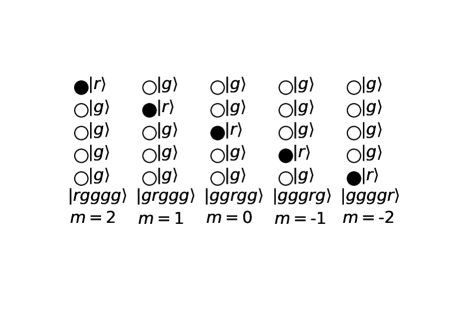
Figure 1: The 5 spin-2 states with a 5 atom setup.

With current technology, it is difficult to get 5 atoms on a line close enough to make the blockade mechanism efficient. However it seems possible to do it with three atoms as in a spin-1 truncation. In the following we will concentrate on this simpler realization.

III.3 Spin-1 CARA implementations

For spin-1, we propose the correspondence

$$\ket{1}\rightarrow\ket{rgg},$$

$$\ket{0}\rightarrow\ket{grg},$$ (21)

$$\ket{-1}\rightarrow\ket{ggr}.$$

This is illustrated in Fig. 2. Again, charge conjugation is implemented as a reflection with respect to the horizontal axis.

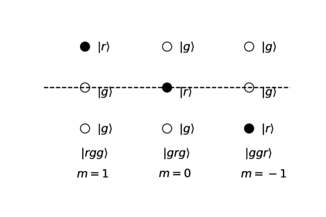
Figure 2: Three spin-1 states with the three atom setup, the 5 other possible states are not displayed.

An even simpler setup consists in using only two Rydberg atoms and having $\ket{m=0}$ to be a state without Rydberg states, namely

$$\ket{1}\rightarrow\ket{rg},$$

$$\ket{0}\rightarrow\ket{gg},$$ (22)

$$\ket{-1}\rightarrow\ket{gr}.$$

This is illustrated in Fig. 3.

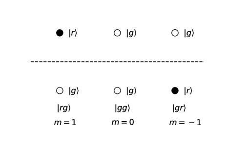
Figure 3: Spin-1 states with the two atom setup.

Since this second possibility is the simplest, it will be the starting point of the presentation of the next sections.

IV One spin system

In this section, we discuss the one spin-1 Hilbert space and the local Hamiltonian for the target model and the CARA implementations with two and three atoms.

IV.1 Target model

The local part of the target Hamiltonian is

$$H^{1T}=\frac{U}{2}(L^{z})^{2}-XU^{x}.$$ (23)

We will discuss the spectrum of this Hamiltonian with emphasis on the symmetries in order to build matching simulators. Since $H^{1T}$ is invariant under charge conjugation, we introduce the $\mathcal{C}$ eigenstates

$$\ket{\pm}\equiv\frac{1}{\sqrt{2}}(\ket{1}\pm\ket{-1}).$$ (24)

with $\mathcal{C}$-eigenvalues $\pm 1$:

$$\mathcal{C}\ket{\pm}=\pm\ket{\pm}.$$ (25)

They are also eigenstates of $(L^{z})^{2}$ with eigenvalue 1. Note that

$$L^{z}\ket{\pm}=\ket{\mp}.$$ (26)

In addition $\mathcal{C}\ket{0}=\ket{0}$.

There is only one $\mathcal{C}$-odd state which is $\ket{-}$. It is annihilated by $U^{x}$

$$U^{x}\ket{-}=0.$$ (27)

Consequently,

$$H^{1T}\ket{-}=\frac{U}{2}\ket{-},$$ (28)

for any value of $X$.

In the $\mathcal{C}$-even sector, we have

$$U^{x}\ket{0}=\frac{1}{\sqrt{2}}\ket{+},$$ (29)

$$U^{x}\ket{+}=\frac{1}{\sqrt{2}}\ket{0},$$ (30)

and the eigenvalues are obtained from the even matrix in the $\ket{0},\ \ket{+}$ basis:

$$H^{1T}_{even}=\begin{pmatrix}0&-\frac{X}{\sqrt{2}}\\ -\frac{X}{\sqrt{2}}&\frac{U}{2}\end{pmatrix}.$$ (31)

The two eigenstates are

$$\ket{0}_{X}=\cos\phi\ket{0}+\sin\phi\ket{+},$$ (32)

with eigenvalue

$$E_{0}(X)=\frac{1}{4}(U-\sqrt{U^{2}+8X^{2}}\ ),$$ (33)

and

$$\ket{+}_{X}=\cos\phi\ket{+}-\sin\phi\ket{0},$$ (34)

with eigenvalue

$$E_{+}(X)=\frac{1}{4}(U+\sqrt{U^{2}+8X^{2}}\ ).$$ (35)

The mixing angle obeys the equation

$$\tan\phi=-\sqrt{2\ }\frac{E_{0}(X)}{X}.$$ (36)

If we treat $X$ as a perturbation, we obtain that at the lowest nontrivial order

$$E_{0}(X) \simeq-\frac{X^{2}}{U},$$ (37)

$$E_{+}(X) \simeq\frac{U}{2}+\frac{X^{2}}{U},$$ (38)

$$\phi \simeq\sqrt{2}\frac{X}{U}.$$ (39)

These results can also be derived using standard perturbative formulas Sakurai (1994). The perturbation has no diagonal element and the energy corrections occur at second order.

IV.2 Two Rydberg atom implementation

The two atom setup discussed in Sec. III.3 provides a very simple implementation of a single spin-1 system. Introducing $\pm 1$ labels for the top and bottom atoms, we call $n_{\pm 1}$ the occupation of their $\ket{r}$ state. The list of the possible states and their occupations are given in Table 1.

Setup	Ket	$n_{+1}$	$n_{-1}$	Short	Energy ($\Omega=0)$
$\begin{matrix}\bullet\\ \circ\end{matrix}$	$\ket{rg}$	1	0	$\ket{1}$	$-\Delta$
$\begin{matrix}\circ\\ \circ\end{matrix}$	$\ket{gg}$	0	0	$\ket{0}$	0
$\begin{matrix}\circ\\ \bullet\end{matrix}$	$\ket{gr}$	0	1	$\ket{-1}$	$-\Delta$
$\begin{matrix}\bullet\\ \bullet\end{matrix}$	$\ket{rr}$	1	1	$\ket{2}$	$-2\Delta+V_{0}$

Table 1: Graphical representation of the two atoms in space, the symbol $\circ$ represents the ground state $\ket{g}$ and $\bullet$ the Rydberg state $\ket{r}$, ket notation, occupations, short notation and energy for $\Omega=0.$

The Hamiltonian for the physical two-atom system is

$$H^{2R}= -\Delta(n_{+1}+n_{-1})+V_{0}n_{+1}n_{-1}$$ (40)

$$+\frac{\Omega}{2}\sum_{\pm 1}(\ket{g_{\pm 1}}\bra{r_{\pm 1}}+\ket{r_{\pm 1}}\bra{g_{\pm 1}}).$$ (41)

We want to match this Hamiltonian with the target $H^{1T}$. We first consider the first term of the target Hamiltonian. The splitting between $\ket{0}$ and $\ket{\pm 1}$ is $\frac{U}{2}$ when $\Omega=0$, and can be implemented by setting

$$\Delta=-\frac{U}{2}.$$ (42)

In addition we want to suppress transitions to the $\ket{rr}$ state by introducing a large enough energy $V_{0}$. This is the blockade mechanism. This can be achieved by positioning the two atoms close enough to each other.

In order to determine $\Omega$, we compare the action of

$$H_{1}^{2R}=\frac{1}{2}\sum_{\pm 1}(\ket{g_{\pm 1}}\bra{r_{\pm 1}}+\ket{r_{\pm 1}}\bra{g_{\pm 1}})$$ (43)

on the simulator Hilbert space to the action of $U^{x}$ on the target Hilbert space.

$$H_{1}^{2R}\ket{gg} =\frac{1}{2}(\ket{rg}+\ket{gr}),$$ (44)

$$H_{1}^{2R}\frac{1}{\sqrt{2}}(\ket{rg}+\ket{gr}) =\frac{1}{\sqrt{2}}(\ket{gg}+\ket{rr}),$$ (45)

$$H_{1}^{2R}\frac{1}{\sqrt{2}}(\ket{rg}-\ket{gr}) =0.$$ (46)

Comparing with the action of $U^{x}$ on the three states of the target Hilbert space, we see that, except for the heavy state $\ket{rr}$, they are identical. Consequently, we can set

$$\Omega=-X.$$ (47)

Except for possible transitions to $\ket{rr}$, the correspondence is exact and the linear formula applies for arbitrary values of $X$. The good matching for $U=1$ with $X=0.5$ and $U=1$ with $X=1.5$ is demonstrated in Fig. 4.

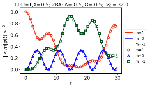
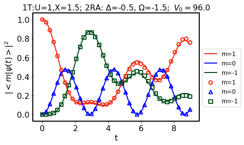
Figure 4: $|\bra{m}U(t)\ket{m=1}|^{2}$, one site with exact Hamiltonian $U=1,\ X=0.5$ (solid lines) and Rydberg Hamiltonian with $\Omega=-0.5$, $\Delta=-0.5$ and $V_{0}=64|\Omega|=32$ (empty symbols) (top), and $U=1,\ X=1.5$ (solid lines) and Rydberg Hamiltonian $H^{2R}$ with $\Omega=-1.5$, $\Delta=-0.5$ and $V_{0}=64|\Omega|=96$ (empty symbols) (bottom).

IV.3 Three Rydberg atom simulator

In the three atom setup, we have an additional atom which is associated with the $m=0$ state. We label its $\ket{r}$ occupation $n_{0}$. The Hamiltonian reads

$$H^{3R}= -\Delta_{0}n_{0}-\Delta\sum_{j=0,\pm 1}n_{j}$$ (48)

$$+V_{0}(n_{0}n_{+1}+n_{0}n_{-1})+V_{0}^{\prime}n_{+1}n_{-1}$$ (49)

$$+\frac{\Omega}{2}\sum_{j=0,\pm 1}(\ket{g_{j}}\bra{r_{j}}+\ket{r_{j}}\bra{g_{j}}),$$ (50)

with

$$V^{\prime}_{0}=\frac{V_{0}}{64}$$ (51)

when the three atoms are located equidistantly on a line as in Fig . 2. The spin-1 sector is shown in Table 2.

Setup	Ket	Energy ($\Omega=0$)
$\begin{matrix}\bullet\\ \circ\\ \circ\end{matrix}$	$\ket{1}$	$-\Delta$
$\begin{matrix}\circ\\ \bullet\\ \circ\end{matrix}$	$\ket{0}$	$-\Delta-\Delta_{0}$
$\begin{matrix}\circ\\ \circ\\ \bullet\end{matrix}$	$\ket{-1}$	$-\Delta$

Table 2: Spin-1 states for the three atom simulator.

The auxiliary sector has five states shown in Table 3.

Setup	Ket	Energy ($\Omega=0$)
$\begin{matrix}\circ\\ \circ\\ \circ\end{matrix}$	$\ket{0^{\prime\prime}}$	0
$\begin{matrix}\bullet\\ \bullet\\ \circ\end{matrix}$	$\ket{1^{\prime}}$	$-2\Delta-\Delta_{0}+V_{0}$
$\begin{matrix}\bullet\\ \circ\\ \bullet\end{matrix}$	$\ket{0^{\prime}}$	$-2\Delta+\frac{V_{0}}{64}$
$\begin{matrix}\circ\\ \bullet\\ \bullet\end{matrix}$	$\ket{-1^{\prime}}$	$-2\Delta-\Delta_{0}+V_{0}$
$\begin{matrix}\bullet\\ \bullet\\ \bullet\end{matrix}$	$\ket{3}$	$-3\Delta-\Delta_{0}+2V_{0}+\frac{V_{0}}{64}$

Table 3: Auxiliary states for the three atom simulator.

Following previous notation, we also define

$$\ket{\pm^{\prime}}\equiv\frac{1}{\sqrt{2}}(\ket{1^{\prime}}\pm\ket{-1^{\prime}}),$$ (52)

and

$$H^{3R}_{1}=\frac{1}{2}\sum_{j=0,\pm 1}(\ket{g_{j}}\bra{r_{j}}+\ket{r_{j}}\bra{g_{j}}),$$ (53)

Unlike the previous situation with two atoms, $H^{3R}_{1}$ only connects the spin-1 sector with the auxiliary sector

$$H^{3R}_{1}\ket{0} =\frac{1}{2}\ket{0^{\prime\prime}}+\frac{1}{\sqrt{2}}\ket{+^{\prime}},$$ (54)

$$H^{3R}_{1}\ket{+} =\frac{1}{2}\ket{+^{\prime}}+\frac{1}{\sqrt{2}}\ket{0^{\prime}}+\frac{1}{\sqrt{2}}\ket{0^{\prime\prime}},$$ (55)

$$H^{3R}_{1}\ket{-} =\frac{1}{2}\ket{-^{\prime}}.$$ (56)

Using the corresponding matrix elements together with standard perturbation theory Sakurai (1994), we obtain the perturbative matching equation for the energy differences:

$$\frac{X^{2}}{U} =\frac{\Omega^{2}}{2}(\frac{1}{\Delta-\frac{V_{0}}{64}}-\frac{1}{\Delta}),$$ (57)

$$\frac{U}{2}+\frac{X^{2}}{U} =\Delta_{0}+\frac{\Omega^{2}}{4}(\frac{1}{\Delta+\Delta_{0}}+\frac{2}{V_{0}-\Delta}-\frac{1}{V_{0}-\Delta-\Delta_{0}}).$$

Similarly we can try to match perturbative expressions for the mixing angle $\phi$ defined in Eq. (36). However, $\phi$ contributions appear at first order in $X$ in the target model (because $U^{x}$ connects $\ket{0}$ and $\ket{+}$), but only at second order in $\Omega$ in the three-atom simulator. More explicitly,

$$\sqrt{2}\frac{X}{U}=\frac{\Omega^{2}}{2\sqrt{2}\Delta_{0}}(\frac{1}{\Delta}+\frac{1}{V_{0}-\Delta-\Delta_{0}}).$$ (58)

This apparently contradicts the idea that $X$ and $\Omega$ should be proportional for small values of $X$. If we are given $U$ and $X$, we have three nonlinear equations for $\Omega$, $\Delta$ , $\Delta_{0}$ and $V_{0}$ and generically, we expect one-parameter families of solutions. By fixing one of the unknowns, one can look for solutions using Newton’s method. More generally, it is easy to find accurate numerical solutions for the energies and mixing of the simulators and it seems possible to attack the matching problem non perturbatively. In order to pursue such effort, it would be useful to know the range of values corresponding to feasible experiments.

With today’s technology, it seems difficult to create non homogeneous detuning and we should consider the limit where $\Delta_{0}$ is zero. In this limit, $\ket{0}$ and $\ket{+}$ are degenerate when $\Omega$ is set to zero. In the $\ket{0}$ and $\ket{+}$ basis, the energy matrix up to second order in $\Omega$ has the form

$$-\Delta\mathbb{1}-\frac{\Omega^{2}}{4}\mathbb{M},$$ (59)

with

$$\mathbb{M}=\begin{pmatrix}\frac{1}{\Delta}+\frac{2}{V_{0}-\Delta}&\frac{\sqrt{2}}{\Delta}+\frac{\sqrt{2}}{V_{0}-\Delta}\\ \frac{\sqrt{2}}{\Delta}+\frac{\sqrt{2}}{V_{0}-\Delta}&\frac{2}{\Delta}+\frac{1}{V_{0}-\Delta}-\frac{2}{\Delta-\frac{V_{0}}{64}}\end{pmatrix}.$$ (60)

The matrix $\mathbb{M}$ determines the mixing angle and the eigenvalues.

IV.4 An example of approximate solution with three Rydberg atoms

The three-atom simulator leads to nonlinear equations. However, it is not difficult to find approximate solutions when $\Delta$ and $V_{0}$ are in a specific ratio. As a simple example, we picked

$$\Delta_{0}=0\ {\rm and}\ V_{0}=2\Delta.$$ (61)

If we neglect the $\frac{V_{0}}{64}$ term, we have

$$\mathbb{M}\simeq\frac{1}{\Delta}\begin{pmatrix}3&2\sqrt{2}\\ 2\sqrt{2}\ &1\end{pmatrix}.$$ (62)

Given that there is an overall minus sign in front of $\mathbb{M}$, its largest eigenvalue corresponds to the lowest energy state and the mixing angle approximately satisfies the equation

$$\tan\phi\simeq\frac{1}{\sqrt{2}}$$ (63)

Comparing with Eq. (36), we find that this angle corresponds to the situation $X=U$. Note that for this significant value $X/U=1$, the angle is not small and the linear approximation of Eq. (36) given in Eq. (39) is not accurate. Instead, we used the exact value of $E_{0}$ given in Eq. (33). For the simulator, this large mixing angle is not controlled by $\Omega^{2}$. This is a feature of degenerate perturbation theory. This procedure is justified by the good quality of the agreement between target and simulator shown in Fig. 5.

Furthermore, we can compute the energy spectrum in this simple example. The eigenvalues of $\mathbb{M}$ are approximately $5/\Delta$ and $-1/\Delta$. In addition, we have up to second order in $\Omega$:

$$E_{-}=-\Delta-\frac{\Omega^{2}}{4}\frac{1}{V_{0}-\Delta}.$$ (64)

Consequently, in this simple example, we have

$$E_{+}-E_{0} =\frac{3}{2}\frac{\Omega^{2}}{\Delta},$$ (65)

$$E_{-}-E_{0} =\frac{\Omega^{2}}{\Delta}.$$ (66)

In the target model with $X=U$, we have

$$E_{+}-E_{0} =\frac{3}{2}U,$$ (67)

$$E_{-}-E_{0} =U.$$ (68)

The ratio of differences are both 3/2 and we can match the scale for $\Omega^{2}/\Delta=U$. Given that the matrix has been approximated, we should look for matching in the region $X\simeq U$. As a numerical example, we used $\Omega=1$, $\Delta=15$ and $V_{0}=30$ and found good matching for $U=0.064,\ X=0.067$ both close to $1/15=0.0666...$ This is illustrated in Fig. 5. Note that the time scale in $1/\Omega$ units is significantly larger than in the two atom case. This is due to the extra $\Omega/\Delta$ factor in the energy scale.

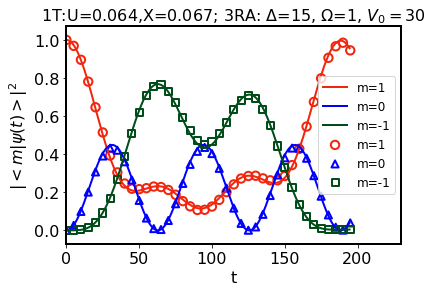
Figure 5: $|\bra{m}U(t)\ket{m=1}|^{2}$ for one site with exact Hamiltonian $U=0.064,\ X=0.067$ (solid lines), Rydberg Hamiltonian with $\Omega=1$, $\Delta=15$ and $V_{0}=30$ (empty symbols).

V Two-spin system

In this section, we follow the same sequence as in Sec. IV for a two-spin system motivated by the Hamiltonian of Eq. (II.2).

V.1 Target model

For the target model we consider two spins called left (L) and right (R) connected by a $Y$-term. The target Hamiltonian for the two-spin system is chosen to be

$$H^{2T}= H^{1T}_{L}+H^{1T}_{R}+\frac{Y}{2}(L_{L}^{z}-L_{R}^{z})^{2}$$ (69)

$$= \frac{U}{2}((L_{L}^{z})^{2}+(L_{R}^{z})^{2})-X(U_{R}^{x}+U_{L}^{x})+\frac{Y}{2}(L_{L}^{z}-L_{R}^{z})^{2}$$

For the time evolution we consider an initial state $\ket{0,0}$, and calculate the probability to stay in that state or to be in the state

$$\ket{S}\equiv\frac{1}{2}(\ket{0,1}+\ket{0,-1}+\ket{1,0}+\ket{-1,0}).$$ (70)

obtained by applying the $X$-term on the initial state. This guarantees a significant overlap when $X$ is not too small. For the comparison of the four and six atom simulators we picked a special target situation where solutions of the one-spin problems are available, more specifically we picked $U=1$, $X=1.2$ and $Y=0.2$.

V.2 Four Rydberg atom simulator

For a simulator with four atoms, we use the two-atom setup for two pairs and include the additional $V_{ij}$ appearing in Eq. (19). The Hamiltonian reads

$$H^{4R}= H^{2R}_{L}+H^{2R}_{R}$$

$$+V_{1}(n_{+1L}n_{-1R}+n_{-1L}n_{+1R})$$ (71)

$$+V_{2}(n_{+1L}n_{+1R}+n_{-1L}n_{-1R})$$

When the $V_{i}$ are positive, we need to have the opposite signs closer (bipartite charge conjugations on alternate sites). In other words, if the interactions are repulsive and decreasing like $1/r^{6}$, we need to put atoms with the same $m$ farther apart. This is illustrated in Fig. 6.

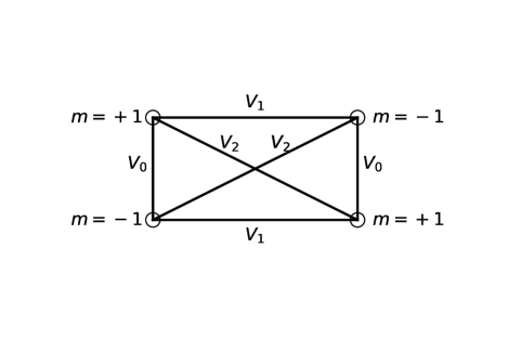
Figure 6: Rydberg interactions for the four atom simulator.

For the standard $1/r^{6}$ Rydberg interactions as in Eq. (20), and using $a_{r}$ and $a_{s}$ as the vertical (as in one spin) and horizontal (coupling the two spins) lattice spacings respectively, and their ratio

$$\rho\equiv\frac{a_{r}}{a_{s}},$$ (72)

we have

$$V_{1}= V_{0}\rho^{6},$$ (73)

$$V_{2}= V_{0}(\rho/\sqrt{1+\rho^{2}}\ )^{6}.$$ (74)

The matching condition when $X=\Omega=0$ reads

$$\Delta =-\frac{U}{2}-\frac{Y}{2},$$ (75)

$$V_{1} =Y,$$ (76)

$$V_{2} =-Y.$$ (77)

The second equation can be solved using

$$\rho=(\frac{Y}{V_{0}})^{1/6}.$$ (78)

The third equation has no solutions for positive $V_{2}$. In Eq. (73) $V_{2}$ is smaller than $V_{1}$ but nevertheles positive. This implies that it is not possible to exactly match the energy of the states $\ket{+1,-1}$ and $\ket{-1,+1}$. The possible solutions to this problem are: 1) ask experimentalists to adjust the couplings locally, 2) consider $Y$-perturbations over situations with non-zero $\Omega$. On the other hand, the phase structure and dynamical features of the simulator are worth exploring even if the matching with the target is not perfect. Note that for the six-atom setup discussed below, we will see that the matching in the limit $\Omega=X=0$ is approximately possible following the mechanism invoked in Ref. Zhang et al. (2018).

In order to give an idea of the size of the effects discussed above for the four atom system, we have considered the problem mentioned in the target section, first with the futuristic $V_{2}=-Y$ (the agreement is excellent) and then with $V_{2}$ is as in Eq. (73) (deviations from exact are quite visible for $t\gtrsim 3$). The results are displayed in Fig. 7.

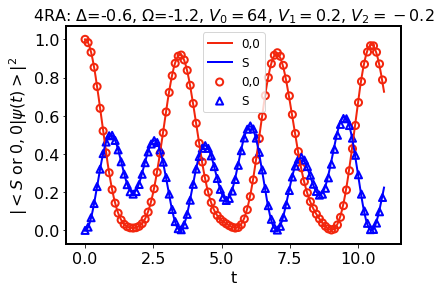
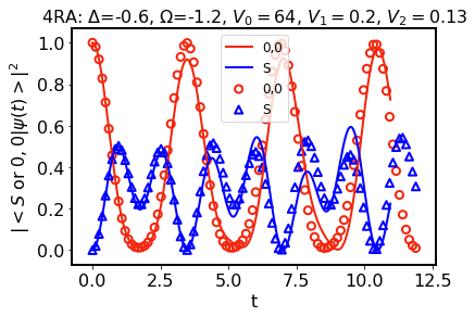
Figure 7: $|\bra{0,0}U(t)\ket{0,0}|^{2}$ and $|\bra{S}U(t)\ket{0,0}|^{2}$, with $\ket{S}$ defined in Eq. (70), for the target two-spin Hamiltonian with $U=1$, $X=1.2$ and $Y=0.2$ (solid lines) and the four atom simulator with $\Delta$=-0.6, $\Omega$=-1.2, $V_{0}=64$, $V_{1}=0.2$, with $V_{2}=-0.2$ (top) and $V_{2}=0.13$ (bottom).

V.3 Six Rydberg atom implementation

We now consider a six-atom setup with two three-atom spin-1 setups. The Hamiltonian reads

$$H^{6R}= H^{3R}_{L}+H^{3R}_{R}$$

$$+V_{1}(n_{+1L}n_{-1R}+n_{-1L}n_{+1R})$$

$$+V_{2}(n_{0L}(n_{+1R}+n_{-1R}))$$ (79)

$$+V_{2}((n_{+1L}+n_{-1L})n_{0R})$$

$$+V_{3}(n_{+1L}n_{+1R}+n_{-1L}n_{-1R})$$

When the $V_{i}$ are positive, we again need to have the atoms representing spins of opposite signs closer in space. This is illustrated in Fig. 8.

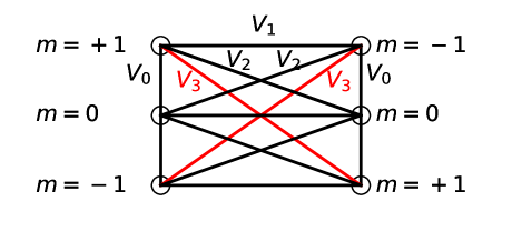
Figure 8: Rydberg interactions for the six atom simulator.

For the standard Rydberg interactions of Eq. (20), we have $V_{1}$ and $V_{2}$ as in Eq. (73) and

$$V_{3}=V_{0}(\rho/\sqrt{1+4\rho^{2}}\ )^{6}$$ (80)

Matching condition when $X=\Omega=0$ are

$$\Delta_{0} =\frac{U}{2}+Y$$

$$V_{1}-V_{2} =\frac{Y}{2}$$ (81)

$$V_{1}-V_{3} =2Y,$$

These equations have approximate solutions with a tuned $\rho$ when $Y$ is not too large. In Fig. 9, we used $\Delta$=15, $\Omega$=1, $V_{0}=30$, and empirically tuned $\rho$ to a value 0.326. A rescaling $K=0.05464$ has been applied to the simulator time to match the target evolution. In Fig. 9, we show the case $\Delta$=15, $\Omega$=1, $V_{0}=30$, as in the one spin-1, with $\rho$=0.326.

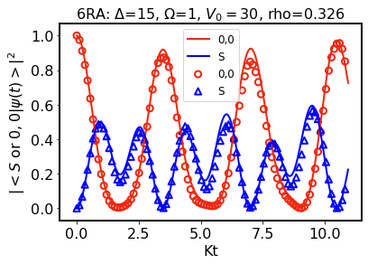
Figure 9: $|\bra{0,0}U(t)\ket{0,0}|^{2}$ and $|\bra{S}U(t)\ket{0,0}|^{2}$, with $\ket{S}$ defined in Eq. (70), with the target two-spin Hamiltonian with $U=1$, $X=1.2$ and $Y=0.2$ (solid lines) and the six atom simulator with $\Delta$=15, $\Omega$=1, $V_{0}=30$, $\rho$=0.326. A rescaling $K=0.05464$ has been applied to the simulator time to match the target evolution.

VI Digital implementations

So far we have discussed an analog simulator with a computational basis given by the states $\ket{g}$ and $\ket{r}$ for each atom. However, it is also possible to calculate the time evolution corresponding to the Rydberg atom Hamiltonians $H^{nR}$ using digital methods, for instance a universal quantum computer with qubits. Before going farther, it should be mentioned that a large $V_{0}$ requires small Trotter steps (of order $1/V_{0}$) in order to suppress the contributions with multiple $\ket{r}$ states by fast oscillations. This is not optimal with NISQ machines and it would be profitable to find a native way to implement the blockade. However, we will discuss the results to give an idea of the time scales involved.

As a simple example, we considered the two atom Hamiltonian $H^{2R}$ with the values $\Omega=-1.5$, $\Delta=-0.5$ as in Fig. 4, but with a lower value $V_{0}=10$. We used a Trotter step $\delta t=0.1=1/V_{0}$. We used Qiskit with the classical simulator called with the instruction Aer.get_backend(’qasm_simulator’) and which sample the so-called statevector Anis (2021). This simulator does not include a realistic noise model corresponding to current hardware such as, for instance, ibmq_lima. The circuit is shown in Fig. 10 with Qiskit notations. We used 1,000 shots for each of the times.

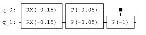
Figure 10: Qiskit circuit for a Trotter form of the evolution operator for $H^{2R}$ described in the text .

In Fig. 10, $P$ is the phase gate

$$P(\phi)\equiv\begin{pmatrix}1&0\\ 0&\exp(i\phi)\end{pmatrix},$$ (82)

and we have the usual definition

$$RX(\lambda)\equiv\exp(-i\frac{\lambda}{2}X).$$ (83)

The results of the Qiskit simulations are shown in Fig. 11. The Trotter errors become quite significant when $t\gtrsim 2$. Based on recent runs on IBMQ Gustafson et al. (2021b), we would expect that computations on actual IBMQ hardware with a slightly larger Trotter step would lead to reasonable results for $t\lesssim 1$. The two spin system can be implemented with universal quantum computers provided that an all-to-all connectivity is available. Hardware considerations will be discussed in a separate paper.

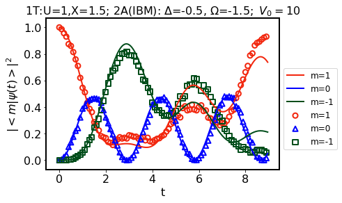
Figure 11: $|\bra{m}U(t)\ket{m=1}|^{2}$, one site with exact Hamiltonian $U=1,\ X=1.5$ (solid lines) and Rydberg Hamiltonian $H^{2R}$ with $\Omega=-1.5$, $\Delta=-0.5$ and $V_{0}=10$, with the circuit of Fig. 10 calculated with the Qiskit simulator (empty symbols).

VII Conclusions

In summary, we have proposed a ladder-shaped CARA with two and three atoms for a single spin-1 and four and six atoms for two coupled spins. In one spatial dimension this is all we need to control in order to study larger systems. We compared target and simulators using perturbative and numerical methods. The two-atom setup provides an easily controllable simulator of the one-spin model while the three-atom setup involves a nonlinear matching. However when two spins are coupled, the six-atom simulator provides solutions closer to the target than the four-atom simulator for small $\Omega$. Approximate implementations of the two-spin model appear to be possible with near term technology. Extensions to spin-2 and implementations in 2+1 dimensions are under investigation.

Acknowledgments. This work is supported in part by the U.S. Department of Energy (DoE) under Award Number DE-SC0019139. Special thanks to Alex Keesling who enthusiastically supported the idea using the Rabi driven term to replace the tunneling in the orginal formulation and made very interesting suggestions. We also thank Shan-Wen Tsai, Jin Zhang, Johannes Zeiher, James Corona, Erik Gustafson, Denis Candido, Michael Flatte, Craig Pryor, Nate Gemelke, Tout Wang, Shangtao Wang and the members of QuLAT for suggestions and comments.

References

- Zhang et al. (2018) J. Zhang, J. Unmuth-Yockey, J. Zeiher, A. Bazavov, S. W. Tsai, and Y. Meurice, Phys. Rev. Lett. 121, 223201 (2018), arXiv:1803.11166 [hep-lat] .
- Bañuls et al. (2020) M. C. Bañuls, R. Blatt, J. Catani, A. Celi, J. I. Cirac, M. Dalmonte, L. Fallani, K. Jansen, M. Lewenstein, S. Montangero, C. A. Muschik, B. Reznik, E. Rico, L. Tagliacozzo, K. Van Acoleyen, F. Verstraete, U.-J. Wiese, M. Wingate, J. Zakrzewski, and P. Zoller, European Physical Journal D 74, 165 (2020), arXiv:1911.00003 [quant-ph] .
- Klco et al. (2021) N. Klco, A. Roggero, and M. J. Savage, (2021), arXiv:2107.04769 [quant-ph] .
- Aidelsburger et al. (2021) M. Aidelsburger et al., (2021), arXiv:2106.03063 [cond-mat.quant-gas] .
- Wiese (2021) U.-J. Wiese, (2021), arXiv:2107.09335 [hep-lat] .
- Gustafson et al. (2021a) E. Gustafson, Y. Zhu, P. Dreher, N. M. Linke, and Y. Meurice, Phys. Rev. D 104, 054507 (2021a), arXiv:2103.06848 [hep-lat] .
- Lamm et al. (2019) H. Lamm, S. Lawrence, and Y. Yamauchi (NuQS), Phys. Rev. D 100, 034518 (2019), arXiv:1903.08807 [hep-lat] .
- Gustafson and Lamm (2021) E. J. Gustafson and H. Lamm, Phys. Rev. D 103, 054507 (2021), arXiv:2011.11677 [hep-lat] .
- Brower et al. (2020) R. C. Brower, D. Berenstein, and H. Kawai, PoS LATTICE2019, 112 (2020), arXiv:2002.10028 [hep-lat] .
- Zohar et al. (2016) E. Zohar, J. I. Cirac, and B. Reznik, Rept. Prog. Phys. 79, 014401 (2016), arXiv:1503.02312 [quant-ph] .
- Wiese (2013) U.-J. Wiese, Annalen Phys. 525, 777 (2013), arXiv:1305.1602 [quant-ph] .
- Zohar and Reznik (2011) E. Zohar and B. Reznik, Phys. Rev. Lett. 107, 275301 (2011), arXiv:1108.1562 [quant-ph] .
- Tagliacozzo et al. (2013) L. Tagliacozzo, A. Celi, A. Zamora, and M. Lewenstein, Annals Phys. 330, 160 (2013), arXiv:1205.0496 [cond-mat.quant-gas] .
- Bañuls et al. (2013) M. C. Bañuls, K. Cichy, K. Jansen, and J. I. Cirac, JHEP 11, 158 (2013), arXiv:1305.3765 [hep-lat] .
- Buyens et al. (2016) B. Buyens, J. Haegeman, H. Verschelde, F. Verstraete, and K. Van Acoleyen, Phys. Rev. X 6, 041040 (2016), arXiv:1509.00246 [hep-lat] .
- Bañuls et al. (2016) M. C. Bañuls, K. Cichy, K. Jansen, and H. Saito, Phys. Rev. D 93, 094512 (2016), arXiv:1603.05002 [hep-lat] .
- Funcke et al. (2020) L. Funcke, K. Jansen, and S. Kühn, Phys. Rev. D 101, 054507 (2020), arXiv:1908.00551 [hep-lat] .
- Martinez et al. (2016) E. A. Martinez et al., Nature 534, 516 (2016), arXiv:1605.04570 [quant-ph] .
- Kasper et al. (2017) V. Kasper, F. Hebenstreit, F. Jendrzejewski, M. K. Oberthaler, and J. Berges, New J. Phys. 19, 023030 (2017), arXiv:1608.03480 [cond-mat.quant-gas] .
- Klco et al. (2018) N. Klco, E. F. Dumitrescu, A. J. McCaskey, T. D. Morris, R. C. Pooser, M. Sanz, E. Solano, P. Lougovski, and M. J. Savage, Phys. Rev. A 98, 032331 (2018), arXiv:1803.03326 [quant-ph] .
- Kharzeev and Kikuchi (2020) D. E. Kharzeev and Y. Kikuchi, Phys. Rev. Res. 2, 023342 (2020), arXiv:2001.00698 [hep-ph] .
- Bazavov et al. (2015) A. Bazavov, Y. Meurice, S.-W. Tsai, J. Unmuth-Yockey, and J. Zhang, Phys. Rev. D92, 076003 (2015), arXiv:1503.08354 [hep-lat] .
- Unmuth-Yockey et al. (2018) J. Unmuth-Yockey, J. Zhang, A. Bazavov, Y. Meurice, and S.-W. Tsai, Phys. Rev. D98, 094511 (2018), arXiv:1807.09186 [hep-lat] .
- Meurice et al. (2020) Y. Meurice, R. Sakai, and J. Unmuth-Yockey, (2020), arXiv:2010.06539 [hep-lat] .
- Meurice (2020) Y. Meurice, Phys. Rev. D 102, 014506 (2020), arXiv:2003.10986 [hep-lat] .
- Unmuth-Yockey (2019) J. F. Unmuth-Yockey, Phys. Rev. D 99, 074502 (2019), arXiv:1811.05884 [hep-lat] .
- Bender and Zohar (2020) J. Bender and E. Zohar, Phys. Rev. D 102, 114517 (2020), arXiv:2008.01349 [quant-ph] .
- Meurice (2019) Y. Meurice, Phys. Rev. D 100, 014506 (2019), arXiv:1903.01918 [hep-lat] .
- Zhang et al. (2021) J. Zhang, Y. Meurice, and S.-W. Tsai, Phys. Rev. B 103, 245137 (2021), arXiv:2104.06342 [cond-mat.quant-gas] .
- Hostetler et al. (2021) L. Hostetler, J. Zhang, R. Sakai, J. Unmuth-Yockey, A. Bazavov, and Y. Meurice, (2021), arXiv:2105.10450 [hep-lat] .
- Chanda et al. (2021) T. Chanda, M. Lewenstein, J. Zakrzewski, and L. Tagliacozzo, (2021), arXiv:2107.11656 [hep-th] .
- Bernien et al. (2017) H. Bernien, S. Schwartz, A. Keesling, H. Levine, A. Omran, H. Pichler, S. Choi, A. S. Zibrov, M. Endres, M. Greiner, V. Vuletić, and M. D. Lukin, Nature (London) 551, 579 (2017), arXiv:1707.04344 [quant-ph] .
- Endres et al. (2016) M. Endres, H. Bernien, A. Keesling, H. Levine, E. R. Anschuetz, A. Krajenbrink, C. Senko, V. Vuletic, M. Greiner, and M. D. Lukin, Science 354, 1024 (2016).
- Keesling et al. (2019) A. Keesling et al., Nature 568, 207 (2019), arXiv:1809.05540 [quant-ph] .
- Cong et al. (2021) I. Cong, S.-T. Wang, H. Levine, A. Keesling, and M. D. Lukin, “Hardware-efficient, fault-tolerant quantum computation with rydberg atoms,” (2021), arXiv:2105.13501 [quant-ph] .
- Semeghini et al. (2021) G. Semeghini, H. Levine, A. Keesling, S. Ebadi, T. T. Wang, D. Bluvstein, R. Verresen, H. Pichler, M. Kalinowski, R. Samajdar, A. Omran, S. Sachdev, A. Vishwanath, M. Greiner, V. Vuletic, and M. D. Lukin, “Probing topological spin liquids on a programmable quantum simulator,” (2021), arXiv:2104.04119 [quant-ph] .
- Surace et al. (2020) F. M. Surace, P. P. Mazza, G. Giudici, A. Lerose, A. Gambassi, and M. Dalmonte, Phys. Rev. X 10, 021041 (2020).
- Celi et al. (2020) A. Celi, B. Vermersch, O. Viyuela, H. Pichler, M. D. Lukin, and P. Zoller, Phys. Rev. X 10, 021057 (2020), arXiv:1907.03311 [quant-ph] .
- Notarnicola et al. (2020) S. Notarnicola, M. Collura, and S. Montangero, Phys. Rev. Research 2, 013288 (2020).
- Wu et al. (2021) X. Wu, X. Liang, Y. Tian, F. Yang, C. Chen, Y.-C. Liu, M. K. Tey, and L. You, Chin. Phys. B 30, 020305 (2021), arXiv:2012.10614 [quant-ph] .
- Ciavarella et al. (2021) A. Ciavarella, N. Klco, and M. J. Savage, Phys. Rev. D 103, 094501 (2021), arXiv:2101.10227 [quant-ph] .
- Gustafson (2021) E. Gustafson, Phys. Rev. D 103, 114505 (2021), arXiv:2104.10136 [quant-ph] .
- Li and Meurice (2005) L. Li and Y. Meurice, Phys. Rev. D 71, 016008 (2005), arXiv:hep-lat/0410029 .
- Meurice (2009) Y. Meurice, Phys. Rev. D 80, 054020 (2009), arXiv:0907.2980 [hep-lat] .
- Zeiher et al. (2016) J. Zeiher, R. van Bijnen, P. Schaus, S. Hild, J.-y. Choi, T. Pohl, I. Bloch, and C. Gross, Nature Physics 12, 1095–1099 (2016).
- Sakurai (1994) J. Sakurai, Modern Quantum Mechanics (Addison-Wesley, 1994).
- Anis (2021) M. D. Anis et al., Qiskit: An Open-source Framework for Quantum Computing (2021).
- Gustafson et al. (2021b) E. Gustafson, P. Dreher, Z. Hang, and Y. Meurice, Quantum Science and Technology 6, 045020 (2021b).