Measuring interstellar turbulence in fast radio burst host galaxies

Abstract

Turbulence is a vital part of the interstellar medium (ISM) of galaxies, contributing significantly to galaxy energy budgets and acting as a regulator of star formation. Despite this, little is understood about ISM turbulence empirically. In the Milky Way, multiple tracers are used to reconstruct the density- and velocity-fluctuation power spectra over an enormous range of scales, but questions remain on the nature of these fluctuations at the smallest scales. Even less is known about the ISM of distant galaxies, where only a few tracers of turbulence, such as non-thermal broadening of optical recombination lines, are accessible. We explore the use of radio-wave scattering of fast radio bursts (FRBs) to add a second probe of turbulence in extragalactic galaxies on scales many orders of magnitude smaller than those probed by emission-line widths. We first develop the formalism to compare the scattering measures of FRBs to alternative probes of density and velocity fluctuations in the host-galaxy ISM. We then apply this formalism to three FRBs with detailed host-galaxy analyses in the literature, with the primary motivation of determining whether FRB scattering within the host galaxy probes the same turbulent cascade as the gas seen in H${\rm\alpha}$ emission. In all cases we consider, we find such an association plausible, although in one of these sources, FRB 20121102A, the radio-scattering limit on the turbulent energy is much less constraining than the H${\rm\alpha}$ line width. We anticipate that future FRB surveys, especially those at frequencies below 1 GHz, will find many FRBs that illuminate the small-scale properties of extragalactic ISM.

1 Introduction

Turbulence has long been thought to cause observed density fluctuations in the Galactic interstellar medium (ISM) on sub-AU to tens of parsec scales (Elmegreen & Scalo, 2004; Scalo & Elmegreen, 2004). Models for turbulence in the ISM, from the Kolmogorov (1941) self-similar cascade to Iroshnikov-Kraichnan (Iroshnikov, 1964; Kraichnan, 1965) magneto-hydrodynamic (MHD) turbulence, generally predict a power-law spectrum of density fluctuations between outer and inner length scales ($l_{o}$ and $l_{i}$ respectively). Energy is injected at the outer scale, likely by a combination of supernovae and O-type stars (Norman & Ferrara, 1996; Mac Low & Klessen, 2004; Hill et al., 2012; Krumholz et al., 2018) and MHD instabilities that extract energy from Galactic differential rotation (Sellwood & Balbus, 1999), and dissipated at the inner scale. Turbulence in the cold/warm neutral phases of the ISM likely causes the formation of molecular-cloud structures that are the sites of present-day star formation (McKee & Ostriker, 2007; Lada et al., 2010).

Turbulence in the warm ionized medium (WIM) has been traced for over 50 years (e.g., Rickett, 1970) using observations of radio-wave propagation (Spangler, 2001; Haverkorn & Spangler, 2013) and H${\rm\alpha}$ emission (Haffner et al., 2009). A remarkable finding from these observations is the “big power-law in the sky”: the concordance of several tracers of density fluctuations with a Kolmogorov spectrum ($P(k)\propto k^{-11/3}$, where $k$ is the spatial wavenumber) between outer scales $l_{o}\sim 10^{18}$ m and inner scales $l_{i}\sim 10^{5}$ m (Armstrong et al., 1995; Chepurnov et al., 2010). More precisely, the outer scale has been found to vary from a few parsec in spiral arms and the inner Galaxy (Haverkorn et al., 2004) to $\sim 100$ pc in the interarm regions (Haverkorn et al., 2008), possibly associated with the sizes of HII regions and old supernova-driven bubbles respectively. The observed inner scale likely corresponds to characteristic kinetic scales (ion inertial length or the Larmor radius) in the WIM (Spangler & Gwinn, 1990). Power laws with similar slopes have also been observed in the densest regions of the WIM (Spangler & Cordes, 1988; Rickett et al., 2009). Density fluctuations in the WIM on all scales, and the associated magnetic-field irregularities, are critical to our understanding of cosmic-ray transport and feedback processes in the ISM (Zweibel, 2013; Hopkins et al., 2021; Lazarian & Xu, 2021). Tantalizingly, it may be that the approximate balance between the WIM, magnetic-field, and cosmic-ray pressures observed in the Galactic ISM (Ferrière, 1998) may not be universal in other galaxies (e.g., Beck, 2007; Beck et al., 2020), with interesting implications for feedback in different environments.

The above picture of WIM turbulence is complicated by instances of extreme scattering of radio sources. Radio-wave diagnostics of conditions in the WIM (and the coronal component of the ISM) can be understood in terms of the dispersion relation of a magnetized plasma (e.g., Rybicki & Lightman, 1986):

$$\frac{c^{2}k_{\lambda}^{2}}{\omega^{2}}=1-\frac{\omega_{p}^{2}}{\omega^{2}\pm\omega\omega_{B}},$$ (1)

where $c$ is the vacuum speed of light, $\omega$ is the angular frequency, $k_{\lambda}$ is the wavevector, $\omega_{p}=4\pi n_{e}q_{e}^{2}/m_{e}$ is the plasma frequency ($n_{e}$ is the electron number density, $q_{e}$ is the electron charge, $m_{e}$ is the electron mass), and $\omega_{B}=q_{e}B_{0}/(m_{e}c)$ is the cyclotron frequency ($B_{0}$ is the magnetic-field strength). The sign of the term in the right-hand denominator depends on the sense of circular polarization. Equation 1 implies that radio waves (a) experience different propagation delays at different frequencies, (b) are differentially refracted (i.e., scattered) by a spatially inhomogeneous medium, and (c) in the case of linearly polarized radiation, trace the magnetic field strength through Faraday rotation. Extreme scattering was first observed as few-month chromatic magnification/de-magnification episodes in compact extragalactic radio sources (Fiedler et al., 1987). If caused by spherically symmetric plasma structures, these extreme scattering events (ESEs) are associated with small (0.1–10 AU), dense ($n_{e}\sim 10\mathrm{\,to\,}10^{3}$ cm^-3) features that are over-pressured relative to the 8000 K, $n_{e}\sim 0.1\mathrm{\,to\,}0.5$ cm^-3 WIM. Structures with similar properties have been identified at specific distances along the sightlines of Galactic radio pulsars (Stinebring et al., 2001; Hill et al., 2005; Coles et al., 2015), which have been found to result in highly anisotropic scattering (i.e., the scattering medium has a preferred axis for ray deflections; Walker et al., 2004; Brisken et al., 2010). Anisotropic scattering by structures at just a few parsec from the Earth is also responsible for the extreme scintillations of intra-day variable sources (e.g., Kedziora-Chudczer et al., 1997).

Extreme radio-wave scattering is difficult to reconcile with models for turbulent cascades in the Galactic ISM (Scalo & Elmegreen, 2004). In particular, the localized nature of the dominant scattering medium along the majority of pulsar sightlines (Bhat et al., 2004), and the implied physical properties of the extreme scattering media, cannot be explained by standard turbulence models. This raises serious questions about the physical nature of the observed power-law spectrum of density fluctuations, given that on $\sim$AU scales the spectrum is probed primarily by radio-wave scattering (Armstrong et al., 1995). Furthermore, there are important implications for our understanding of the structure of the WIM, and of the dissipation of energy injected at the observed outer scales of the density-fluctuation spectrum. Anisotropic scattering at least is expected in models for strong turbulence caused by non-linear interactions between Alfvén waves in the WIM (Goldreich & Sridhar, 1995). Folded corrugated sheet-like magnetic structures, motivated physically by numerical simulations of small-scale dynamos (Goldreich & Sridhar, 2006), may explain instances of extreme scattering and solve the over-pressurization problem (Pen & King, 2012; Pen & Levin, 2014).

This paper is motivated by the prospect of comparing tracers of density fluctuations on multiple scales (tens of parsecs to AU) in the WIM of galaxies besides the Milky Way. By doing so, we aim to study multiple instances of density-fluctuation spectra, and thus obtain insights into their astrophysical origins. Pulsars, one of the few types of radio sources sufficiently compact to undergo refractive scintillation, are not luminous enough for their pulsed radio emission to be detected from distant galaxies. However, fast radio bursts (FRBs) associated with specific regions within galaxies (e.g., Bassa et al., 2017; Marcote et al., 2020; Chittidi et al., 2020) offer unique opportunities to probe extragalactic AU-scale density fluctuations.

Since the discovery of FRBs over a decade ago, several hundreds of bursts from more than five hundred FRB sources have been detected. FRBs are dispersed by the ISM of host galaxies, the intergalactic medium (IGM), the circum-galactic medium (CGM) of intervening galaxies, and the halo and interstellar medium (ISM) of the Milky Way (Cordes & Chatterjee, 2019). Density fluctuations along FRB sightlines at any of these locations can also cause FRBs to be observed along multiple paths, resulting in an exponential distribution of burst arrival times. Rays propagating along multiple paths may coherently interfere, resulting in strong spectral modulations. Although such scattering effects are not ubiquitous in FRB samples (Ravi, 2019a), both cases have been observed (e.g. Farah et al., 2018; CHIME/FRB Collaboration et al., 2019a; Day et al., 2020), and in some cases attributed to the host galaxy (Masui et al., 2015) or the IGM (and CGM of intervening galaxies) (Ravi et al., 2016; Cho et al., 2020). FRB scattering promises to provide diagnostics of the characteristics of the density fluctuations in extragalactic plasmas.

In this paper, we develop the formalism to constrain density fluctuations on multiple scales in extragalatic ISM. We do so by comparing measures of FRB scattering with optical recombination-line tracers of their host environments. We start in Section 2 by describing the formalism we will adopt for comparing these two different tracers of turbulence. In Section 3, we discuss ways to determine the location of scattering material, in order to reasonably ensure that the FRB scattering measure is indeed probing the host galaxy environment or material immediately surrounding the FRB source, rather than the Milky Way or intervening galaxy halos. Then, in Section 4, we illustrate the application of the formalism we develop to three FRBs localized to specific regions within their host galaxies with detailed optical follow-up observations. In Section 5 we present some concluding remarks with a focus on targeting future optical and VLBI follow-up campaigns of localized FRBs for understanding extragalactic ISM properties.

2 Probes of turbulence on multiple scales

Studies of turbulence in the Milky Way ISM take advantage of tracers of density and velocity fluctuations on multiple scales. Diffractive scattering of pulsars probes some of the smallest scales of density fluctuations in the Milky Way. Analyses of pulsar scattering have been used to constrain the inner scale, which is the scale at which energy is dissipated from the turbulent cascade (Spangler & Gwinn, 1990; Rickett et al., 2009). At the largest scales, gas velocities, for example from HI velocity maps, can be used to reconstruct the velocity fluctuation structure function (Chepurnov & Lazarian, 2010).

Very few of these tracers are accessible at extragalactic distances. Some galaxies of interest may be sufficiently nearby to study velocity dispersion through maps of, for example, HI emission. When we do not have sufficient spatial resolution to resolve scales below the outer scale, we can instead access the velocity dispersion of ionized gas through broadening of recombination lines. Such a measurement is sensitive to velocity fluctuations on scales below the spatial resolution of the instrument but dominated by the largest contributing scale (i.e., the smaller of the outer scale and the resolution of the instrument). Pulsars, used to probe density fluctuations at the other end of the fluctuation spectrum in the Milky Way, are unfortunately not sufficiently bright to be routinely observed at extragalactic distances.

Diffractive scattering of FRBs probes density fluctuations at the Fresnel scale, the radius of the region in the lens plane that contributes to phase fluctuations for any ray that passes through the lensing material. In the case studies presented in Section 4, the Fresnel scale is $\sim 10^{9}$ m for scattering within the host galaxies. The velocity-widths of emission lines, on the other hand, are sensitive to the outer scale of the turbulent fluctuations, $\sim 10^{18}$ m in our case studies and orders of magnitude larger than the scales probed by scattering.

The power spectrum of turbulent density fluctuations is typically parameterized as a power law,

$$P_{n}(q,l)=C_{n}^{2}(l)q^{-\beta}e^{-q^{2}l_{i}^{2}}$$ (2)

on scales smaller than the outer scale, i.e., for $q<q_{o}$. Here $q=\frac{2\pi}{l}$ is the spatial frequency, $q_{o}=\frac{2\pi}{l_{o}}$, and $l_{i}$ and $l_{o}$ are the inner and outer scales of the density fluctuations. We will use $l$ to represent light travel distances and $d$ for angular diameter distances. The power spectrum of velocity fluctuations takes the same form

$$P_{v}(q,l)=C_{v}^{2}(l)q^{-\beta}e^{-q^{2}l_{i}^{2}}\;,$$ (3)

with the same inner and outer scale but a different fluctution amplitude, $C_{v}$. The velocity fluctuation spectrum is proportional to the energy spectrum (per unit mass),

$$E(q)=2\pi q^{2}P_{v}(q)\propto q^{2-\beta}\;.$$ (4)

When $\beta>2$, the largest scales (smallest $q$) dominate the energy in turbulence. Turbulence in the Milky Way ISM is studied through many different tracers; the amalgamation of these tracers over 11 orders of magnitude is consistent with Kolmogorov turbulence, for which $\beta=11/3$ (Armstrong et al., 1995).

2.1 Density fluctuations and radio-wave scattering

The scattering medium can be characterized by the scattering measure (SM), which is the integral of the density fluctuations along the path through the medium,

$$\mathrm{SM}=\int C_{n}^{2}(l)\mathrm{d}l\;.$$ (5)

Macquart & Koay (2013) generalize the relation between the SM and the diffractive scale, $r_{\mathrm{diff}}$ (the characteristic correlation length of fluctuations in the scattering medium) for scattering at cosmological distances:

$$\mathrm{SM}=\begin{cases}\left(r_{\mathrm{diff}}^{2}\pi r_{e}^{2}\lambda^{2}(1+z_{\mathrm{lens}})^{-2}l_{i}^{\beta-4}\frac{\beta}{4}\Gamma(-\frac{\beta}{2})\right)^{-1}&r_{\mathrm{diff}}<l_{i}\\ \left(r_{\mathrm{diff}}^{\beta-2}2^{2-\beta}\pi r_{e}^{2}\lambda^{2}(1+z_{\mathrm{lens}})^{-2}\beta\frac{\Gamma(-\beta/2)}{\Gamma(\beta/2)}\right)^{-1}&r_{\mathrm{diff}}\gg l_{i}\;.\end{cases}$$ (6)

Here, $r_{e}$ is the classical electron radius and $z_{\mathrm{lens}}$ is the redshift of the scattering material.

The diffractive scale is related to the observed scattering time $\tau$,

$$r_{\mathrm{diff}}=\sqrt{\frac{d_{\mathrm{lens}}d_{\mathrm{lens,src}}}{d_{\mathrm{src}}}\left(\frac{\lambda}{2\pi}\right)^{2}(1+z_{\mathrm{lens}})^{-1}(c\tau)^{-1}}\;,$$ (7)

where $\lambda$ is the observing wavelength. If $r_{\mathrm{diff}}<l_{i}$,

$$\tau=\frac{1}{4\pi c}\frac{d_{\mathrm{lens}}d_{\mathrm{lens,src}}}{d_{\mathrm{src}}}\frac{\lambda^{4}r_{e}^{2}}{(1+z_{\mathrm{lens}})^{3}}l_{i}^{\beta-4}\frac{\beta}{4}\Gamma\left(-\frac{\beta}{2}\right)\mathrm{SM}\;.$$ (8)

Equations (8) and (5) allow us to use FRB scattering to constrain the amplitude of the density fluctuations at the Fresnel scale, $r_{F}$, given by Schneider et al. (1992) and Macquart & Koay (2013) for a cosmological lens

$$r_{F}(z)=\sqrt{\frac{d_{\mathrm{lens}}d_{\mathrm{lens,src}}\lambda_{\mathrm{obs}}}{2\pi d_{\mathrm{src}}(1+z_{\mathrm{lens}})}}\;,$$ (9)

where $\lambda_{\mathrm{obs}}$ is the observing wavelength, and $d_{\mathrm{lens}}$, $d_{\mathrm{lens,src}}$ and $d_{\mathrm{src}}$ are the angular diameter distances between the observer and the scattering screen, the screen and the FRB source, and the observer and the FRB source respectively. Note that $d_{\mathrm{lens,src}}\neq d_{\mathrm{src}}-d_{\mathrm{lens}}$; instead, in a flat Universe,

$$d_{\mathrm{lens,src}}=d_{\mathrm{src}}-\frac{1+z_{\mathrm{lens}}}{1+z_{\mathrm{src}}}d_{\mathrm{lens}}\;,$$ (10)

where $z_{\mathrm{src}}$ is the redshift of the source (Peebles, 1993, pp. 336-337). In this work we focus on cases where the lens is close to the source and $z_{\mathrm{lens}}\approx z_{\mathrm{src}}$, for which we write

$$r_{F}(z) \approx\sqrt{\frac{\lambda}{2\pi}\frac{d_{\mathrm{lens,src}}}{1+z_{\mathrm{src}}}}$$ (11)

$$\approx 3.7\times 10^{8}\,\mathrm{m}\,\left(\frac{f_{\mathrm{obs}}}{1\,\mathrm{GHz}}\right)^{-1/2}\left(\frac{d_{\mathrm{lens,src}}}{100\,\mathrm{pc}}\right)^{1/2}\left(\frac{1+z_{\mathrm{src}}}{1.1}\right)^{-1/2}\;.$$ (12)

Note from the form of equation (8) that temporal scattering is greatest for screens approximately half-way between the observer and the source. At low redshifts, scattering from the Milky Way and the FRB host galaxy is weighted approximately equally, but the additional redshift term will weight scattering in the Milky Way over scattering in the host galaxy for sources at high redshifts.

2.2 Velocity fluctuations and dispersion

Broadening of emission and absorption lines provides a probe of the velocity distribution in the emitting or absorbing gas. This distribution includes thermal and turbulent motions, as well as bulk motion due to, for example, gravitational infall or rotation of a disk. While bulk motion can have a more complex distribution, line broadening due to both thermal and turbulent motions is well-described by a Gaussian broadening function, and the total velocity dispersion is the quadrature sum of the thermal and turbulent velocity dispersions in the absence of bulk motion. In this work, we will use the H$\alpha$ recombination line as our velocity tracer. We assume that the H${\rm\alpha}$-emitting regions do not have significant bulk motions, and we account for only the turbulent and thermal velocity distributions.

Information on the velocity fluctuation spectrum is present in the turbulent contribution to the velocity dispersion. The velocity power spectrum captures the mean-square fluctuations at a scale $q$, and so the variance of the velocity is given by the integral of the power spectrum over all (but the 0^th) scales:

$$\sigma^{2}_{v,nt} =\int_{q_{o}}^{\infty}d^{3}\mathbf{q}P_{v}(\mathbf{q})$$ (13)

$$=2\pi C_{v}^{2}q_{i}^{3-\beta}\,\Gamma\left(\frac{3-\beta}{2},\left(q_{o}l_{i}\right)^{2}\right)\;.$$ (14)

Since $P_{v}(q)\propto q^{-\beta}$, we see that the integral in equation (13) is dominated by large spatial scales when $\beta>2$. (In Kolmogorov turbulence, $\beta=11/3\approx 3.7$). When $\beta<2$, the smallest scales dominate the velocity dispersion and therefore the energy.

Using the relation $\Gamma(s+1,x)=s\Gamma(s,x)+x^{s}e^{-x}$, we can write

$$\Gamma\left(\frac{3-\beta}{2},\left(q_{o}l_{i}\right)^{2}\right) =\frac{2}{\beta-3}\left(q_{o}l_{i}\right)^{\frac{3-\beta}{2}}e^{-\left(q_{o}l_{i}\right)^{2}}-\frac{2}{\beta-3}\Gamma\left(\frac{5-\beta}{2},\left(q_{o}l_{i}\right)^{2}\right)\;.$$ (15)

For $3<\beta<5$ and $q_{o}l_{i}\ll 1$, this simplifies to

$$\Gamma\left(\frac{3-\beta}{2},\left(q_{o}l_{i}\right)^{2}\right)\approx\frac{2}{\beta-3}\left(q_{o}l_{i}\right)^{3-\beta}\;.$$ (16)

and we find

$$\sigma_{v}^{2}\approx\frac{2(2\pi)^{4-\beta}}{\beta-3}C_{v}^{2}l_{o}^{\beta-3}\;,$$ (17)

which more immediately shows the dependence of the velocity dispersion (and the energy) on the outer scale.

2.3 Relating the density and velocity power spectra

If we can relate the amplitude of the velocity fluctuation power spectrum to that of the density power spectrum, we can calculate the turbulent velocity dispersion in the ionized medium from the FRB SM. This assumes: (a) the plasma probed by FRB scattering is part of the same turbulent cascade as the gas emitting in H${\rm\alpha}$; and (b) the turbulent fluctuations follow a power-law spectrum between the scales probed by FRB scattering (the Fresnel scale of the lens, $\sim 10^{8}$ m) and the velocity dispersion (the outer scale). If we equate the outer scale to the size of knots of H$\alpha$ emission close to FRB sources in their host galaxies, we infer outer scales of $\sim 100\,\mathrm{pc}\simeq 3\times 10^{18}$ m, similar to the outer scale in the Milky Way (Armstrong et al., 1995); see Section 4 for further details. If the velocity dispersion anticipated from scattering disagrees with the observed velocity dispersion, at least one of these assumptions must be incorrect.

If the amplitude of the turbulent fluctuations inferred from FRB scattering is much larger than the amplitude inferred from emission line widths, this may suggest that FRBs originate from anomalously highly-scattered environments in their host galaxies. This would be analogous to the case of the Crab pulsar; the Crab nebula is one of the most highly-scattered environments that we observe in the Milky Way. The Crab pulsar exhibits variable scattering timescales up to 600 $\mu$s at 610 MHz (McKee et al., 2018). The variability of this scattering time indicates that scattering is occurring close to the source, likely within the nebula itself. Adopting a distance of 0.5 pc between the source and scattering screen, and assuming a Kolmogorov spectrum with an inner scale of 1000 km, this corresponds to a SM of $\sim$300 kpc m^-20/3 (equation 8). Similarly, underscattering of FRBs compared to expectations from H${\rm\alpha}$ line widths implies that the observed FRBs are in fact not associated with the nearby H${\rm\alpha}$-emitting regions. Associations (or non-associations) of FRBs with star-forming regions are especially impactful for understanding the progenitors of FRB sources.

An alternative explanation for a discrepancy in the turbulent energies inferred from radio-wave scattering and optical line widths is that the assumption that the turbulent power spectrum follows a simple power law with $\beta=11/3$ is incorrect. Inferred departures from $\beta=11/3$ are not unprecedented in the Milky Way. The evolution of some pulsar scattering timescales over frequency ($\tau\propto\nu^{-\alpha}$) suggests a departure from Kolmogorov turbulence; pulsar scattering exponents (of $\alpha\sim 3\,\mathrm{to}\,4$, compared to the Kolmogorov value of $\alpha=4.4$; e.g., Geyer et al., 2017) suggest $\beta>11/3$, and indicate increased power on large scales compared to Kolomogorov turbulence, although it is likely that this effect arises from anisotropic scattering at discrete screens. VLBI observations towards the Galactic center indicate increased power in turbulence on small scales compared to a Kolmogorov spectrum. From the size of the scattered disk of Sgr A* (sensitive to the smallest fluctuations, at the inner scale, $\sim 800\,$km) and refractive substructure in the disk (sensitive to scales of $10^{13}-10^{14}$ cm) Johnson et al. (2018) infer a slope of the density fluctuation power spectrum of $\beta=3.38$. Heightened power near the inner scale is also observed in the density spectrum of the solar wind (Coles et al., 1991), in this case due to a flattening of the power spectrum at small scales. Johnson et al. (2018) note that a similar flattening is consistent with their Sgr A* measurements. Obtaining additional tracers at intermediate scales would allow us to measure the index of the power spectrum and discern breaks or changes in the power-law form. We examine the feasibility of probing density and velocity fluctuations at additional scales for FRB host galaxies in Section 5.

Simulations of isothermal turbulence (e.g. Passot & Vázquez-Semadeni, 1998; Konstandin et al., 2012) show a linear relationship between the standard deviation of the density distribution, $\sigma_{\rho}$, and the rms Mach number, $\mathcal{M}=v_{\mathrm{rms}}/c_{s}$, of the gas,

$$\sigma_{\rho}=b\mathcal{M}\langle\rho\rangle\;,$$ (18)

where $v_{\mathrm{rms}}$ is the rms velocity, $c_{s}$ is the speed of sound in the gas, $\langle\rho\rangle$ is the volume-weighted mean density, and $b$ is a constant. Konstandin et al. (2012) find that, in the supersonic regime, $b=1$ and $b=1/3$ for compressive and solenoidal forcing respectively. A mixture of both types of forcing is likely in the ISM (Federrath et al., 2010); for simplicity we choose a fiducial value $b=1$.

In analogy to equation (14), we can write

$$\sigma_{\delta n_{e}}^{2}=(2\pi)^{4-\beta}C_{n}^{2}q_{o}^{3-\beta}\frac{2}{\beta-3}\;.$$ (19)

This allows us to relate the amplitudes of the velocity and density fluctuations

$$C_{v}^{2}=\left(\frac{c_{s}}{b\langle n_{e}\rangle}\right)^{2}C_{n}^{2}\;,$$ (20)

where $\langle n_{e}\rangle$ is the average electron number density, and also provides a relationship between the velocity dispersion, $\sigma_{v}$, and the amplitude of the velocity perturbation power spectrum.

The emission measure, $\mathrm{EM}$, calculated from the H${\rm\alpha}$ emission line, probes the square of the electron density along the line-of-sight, $\mathrm{EM}=\int n_{e}^{2}\mathrm{d}l$. The EM in a clumpy medium, with electron density fluctuations within the clumps, is related to the mean electron density by (Cordes et al., 2016, equation B3):

$$\mathrm{EM}=\frac{\zeta(1+\epsilon^{2})}{f_{f}}\langle n_{e}\rangle^{2}L_{\mathrm{EM}}\;.$$ (21)

We adopt fiducial values of $\epsilon=1$ and $\zeta=2$ corresponding to complete modulation of the electron density inside the clouds and 100% variation of the average $n_{e}$ between clouds for consistency with Tendulkar et al. (2017). $L_{\mathrm{EM}}$ is the path length through the medium that contributes to the EM and $f_{f}$ is the filling factor of the clouds within the medium.

Using this in equation (20), we can write,

$$C_{v}^{2} =\left(\frac{c_{s}}{b}\right)^{2}\frac{\zeta(1+\epsilon^{2})}{f_{f}f_{r}}\frac{L_{\mathrm{EM}}}{\mathrm{EM}}C_{n}^{2}$$ (22)

$$=\left(\frac{c_{s}}{b}\right)^{2}\frac{\zeta(1+\epsilon^{2})}{f_{f}f_{r}}\frac{\mathrm{SM}}{\mathrm{EM}}\;,$$ (23)

where we have used $\mathrm{SM}=C_{n}^{2}L_{\mathrm{SM}}$ and assumed that the path length that contributes to the SM $L_{\mathrm{SM}}=f_{r}L_{\mathrm{EM}}$, where $f_{r}\leq 1$. This accounts for the possibility that the FRB source is embedded in the scattering medium, in which case a shorter path length will contribute to the SM than to the EM.

We can then write the velocity dispersion as

$$\sigma_{v}^{2} =\frac{2(2\pi)^{4-\beta}}{\beta-3}l_{o}^{\beta-3}\left(\frac{c_{s}}{b}\right)^{2}\frac{\zeta(1+\epsilon^{2})}{f_{f}f_{r}}\frac{\mathrm{SM}}{\mathrm{EM}}$$ (24)

$$=\frac{2(2\pi)^{4-\beta}}{\beta-3}l_{o}^{\beta-3}\left(\frac{c_{s}}{b\,n_{e}}\right)^{2}\frac{4\pi c}{f_{r}}\frac{d_{\mathrm{src}}}{d_{\mathrm{lens}}d_{\mathrm{lens,src}}}\frac{(1+z_{\mathrm{lens}})^{3}}{\lambda^{4}r_{e}^{2}}l_{i}^{4-\beta}\frac{4}{\beta\Gamma(-\beta/2)}\tau\;.$$ (25)

For Kolmogorov ($\beta=11/3$) turbulence,

$$\sigma_{v}^{2} =3(2\pi)^{1/3}l_{o}^{2/3}\left(\frac{c_{s}}{b}\right)^{2}\frac{\zeta(1+\epsilon^{2})}{f_{f}f_{r}}\frac{\mathrm{SM}}{\mathrm{EM}}$$ (26)

$$\begin{split}&=\left(1.4\times 10^{5}\,\mathrm{km}\,\mathrm{s}^{-1}\right)^{2}\left(\frac{l_{o}}{150\,\mathrm{pc}}\right)^{2/3}\left(\frac{c_{s}}{10\,\mathrm{km}\,\mathrm{s}^{-1}}\right)^{2}\left(\frac{b}{1}\right)^{-2}\left(\frac{\zeta}{2}\right)\left(\frac{f_{f}}{0.1}\right)^{-1}\left(\frac{f_{r}}{0.5}\right)^{-1}\left(\frac{1+\epsilon^{2}}{2}\right)\times\\ &\,\,\,\,\,\left(\frac{\mathrm{SM}}{10^{5}\,\mathrm{kpc}\,\mathrm{m}^{-20/3}}\right)\left(\frac{\mathrm{EM}}{600\,\mathrm{pc}\,\mathrm{cm}^{-6}}\right)^{-1}\;.\end{split}$$ (27)

With a measurement of the SM (from radio observations of the FRB) and EM (from optical observations of the host galaxy), combined with an estimate of the path length through the star-forming region, we can directly compare the velocity dispersion predicted from the SM and EM to the velocity dispersion from optical recombination-line widths. We will use a fidicual sound speed of $c_{s}=\sqrt{\frac{kT}{\mu}}=10$ km s^-1, for hydrogen gas at a temperature of $10^{4}$ K. Increased gas metallicities increase the mean molecular weight $\mu$ and decrease the sound speed, but the sound speed is most sensitive to the temperature of the medium. An independent measure of the temperature would allow us to constrain the sound speed more accurately.

If instead we assume that the optical emission lines and the FRB SM are probing the same turbulent spectrum, we can assert that the velocity dispersions inferred from these two tracers must be equal and constrain the nature of the turbulent cascade. Particularly, as $\sigma_{v}^{2}\propto l_{o}^{\beta-3}l_{i}^{4-\beta}n_{e}^{-2}$, we can constrain the inner and outer scales and the index of the turbulent power spectrum through this method. We can also vary the electron density, $n_{e}$; the inference of the average electron density from the EM of the emitting gas depends on the clumpiness of the electrons in the gas, parameterized through the filling factor of ionized gas in the medium and the electron density variations between and within the ionized clouds. Additional constraints on $\langle n_{e}\rangle$ translate to constraints on these clumpiness parameters.

2.4 Energetics of turbulence at the scattering screen

In addition to testing whether FRB scattering and the velocity dispersion of the ionized gas are probing the same plasma and the same turbulent cascade, we can use both observations to estimate the turbulent energy in the region. In this section, we develop the formalism for relating the SM and the velocity dispersion to the turbulent energy. As above, we will consider isotropic turbulence with density and velocity fluctuations described by equations (2) and (3). Since we are considering scattering originating in the host galaxy, the path length through the scattering plasma is only a small percentage of the entire path length between the observer and source, and we will use a thin-screen formalism to relate the FRB SM and the amplitude of the density fluctuation power spectrum.

The energy per unit mass can be calculated from the integral of the the kinetic energy in the velocity fluctuations,

$$E =\frac{1}{2}\int\mathrm{d}^{3}{\bf q}P_{v}(q)$$ (28)

$$=2\pi\int_{q_{o}}^{\infty}C_{v}^{2}q^{2-\beta}e^{-\frac{q^{2}}{q_{i}^{2}}}$$ (29)

$$=\frac{(2\pi)^{4-\beta}}{\beta-3}l_{o}^{\beta-3}\left(\frac{c_{s}}{b}\right)^{2}\frac{\zeta(1+\epsilon^{2})}{f_{f}f_{r}}\frac{\mathrm{SM}}{\mathrm{EM}}$$ (30)

$$=\frac{(2\pi)^{4-\beta}}{\beta-3}l_{o}^{\beta-3}\left(\frac{c_{s}}{b\,n_{e}}\right)^{2}\frac{4\pi c}{f_{r}}\frac{d_{\mathrm{src}}}{d_{\mathrm{lens}}d_{\mathrm{lens,src}}}\frac{(1+z_{\mathrm{lens}})^{3}}{\lambda^{4}r_{e}^{2}}l_{i}^{4-\beta}\frac{4}{\beta\Gamma(-\beta/2)}\tau\;.$$ (31)

For Kolmogorov turbulence,

$$E =\frac{3}{2}(2\pi)^{1/3}l_{o}^{2/3}\left(\frac{c_{s}}{b}\right)^{2}\frac{\zeta(1+\epsilon^{2})}{f_{f}f_{r}}\frac{\mathrm{SM}}{\mathrm{EM}}\;$$ (32)

$$\begin{split}&=2.0\times 10^{53}\,\mathrm{erg}M_{\odot}^{-1}\left(\frac{l_{o}}{150\,\mathrm{pc}}\right)^{2/3}\left(\frac{c_{s}}{10\,\mathrm{km}\,\mathrm{s}^{-1}}\right)^{2}\left(\frac{b}{1}\right)^{-2}\left(\frac{\zeta}{2}\right)\left(\frac{f_{f}}{0.1}\right)^{-1}\left(\frac{f_{r}}{0.5}\right)^{-1}\left(\frac{1+\epsilon^{2}}{2}\right)\times\\ &\,\,\,\,\,\left(\frac{\mathrm{SM}}{10^{5}\,\mathrm{kpc}\,\mathrm{m}^{-20/3}}\right)\left(\frac{\mathrm{EM}}{600\,\mathrm{pc}\,\mathrm{cm}^{-6}}\right)^{-1}\;.\end{split}$$ (33)

Equation (32) can also be written in terms of the non-thermal velocity dispersion as

$$E=\frac{1}{2}\sigma_{v,nt}^{2}\;.$$ (34)

Using this equation, we can also estimate the energy in the turbulence from the non-thermal gas velocity dispersion measured from ionized emission lines.

3 Determining the distance to the scattering plasma

As the radio emission from FRBs propagates towards us, it interacts with the intervening ionized plasma. This includes any plasma associated with the FRB source itself, such as a pulsar wind nebula, supernova remnant or other ejecta from a compact binary merger (e.g. Piro & Gaensler, 2018; Straal et al., 2020; Kundu & Ferrario, 2020; Zhao et al., 2021), the host galaxy ISM, including star-forming and HII regions, the IGM and the CGM of intervening galaxies, halos of the Milky Way and intervening galaxies (Ocker et al., 2021), and the ISM of the Milky Way.

The effects of the Milky Way ISM are constrained observationally by pulsar scattering and dispersion. From these measurements, models of the electron density distribution within the Milky Way ISM, such as the NE2001 model (Cordes & Lazio, 2002, 2003) and the YMW16 model (Yao et al., 2017), have been developed. These include features, such as spiral arms, within the Milky Way and predict the effects of dispersion and scattering in the Milky Way ISM on both galactic and extragalactic radio sources. Using these predictions, we can determine if the scattering observed towards any particular FRB predominantly originates from the Milky Way.

A similar tomography is yet to be realized for the IGM, although FRB dispersion and scattering measurements hold promise for mapping the electron content of the IGM out to high redshifts (e.g. McQuinn, 2014; Zheng et al., 2014; Ravi, 2019b; Caleb et al., 2019). Macquart et al. (2020) present the first DM-$z$ relation constructed from five FRBs with localizations and host-galaxy associations, out to redshifts of $z\sim 0.5$; the trend of this relation describes the mean electron content of the IGM. FRBs that fall outside of this relation may intercept a deficit of ionized electrons due to voids along the light-travel path, or an abundance due to heightened dispersion in the host galaxy, and filaments or CGM of intervening galaxies along the light-travel path. Detailed analyses of individual FRBs have also yielded rich information about scattering in the IGM (Ravi et al., 2016; Cho et al., 2020; Simha et al., 2020), the halos and CGM of intervening galaxies (Prochaska et al., 2019; Connor et al., 2020) and the host galaxy (Masui et al., 2015).

One of the challenges of using FRBs to study density fluctuations in intervening material is attributing extragalactic scattering to the appropriate material along the line-of-sight. This is especially key for in-depth studies of individual systems, where we do not have the opportunity to marginalize over many lines-of-sight and host galaxies. One way to constrain the distance to the scattering material is to use the relationship between angular and temporal broadening, which depends on the distances between the observer and the source and scattering screen. Scattering angles can and have been measured by modelling the scintillation pattern on the Earth (to localize interstellar scattering towards both pulsars (Rickett et al., 2014; Reardon et al., 2019, 2020; Marthi et al., 2020) and AGN (e.g. Bignall et al., 2007; Oosterloo et al., 2020; Wang et al., 2021)), directly through VLBI (to localize interstellar scattering towards pulsars; Brisken et al., 2010; Smirnova et al., 2014; Popov et al., 2016; Shishov et al., 2017; Fadeev et al., 2018), and using size constraints from the presence of scintillation in two-screen scattering systems (applied to FRB scattering to place an upper limit on the source-screen distance; Masui et al., 2015; Farah et al., 2018).

For scattering of emission from a source at an angular diameter distance $d_{\mathrm{src}}$ from the observer by a single thin screen at an angular diameter distance $d_{\mathrm{lens}}$ and redshift $z_{\mathrm{lens}}$ from the observer, the temporal broadening $\tau$, angular broadening $\theta$ and scintillation bandwidth $\Delta\nu$ are related by (see Appendix A)

$$\tau\simeq\frac{1}{c}\frac{d_{\mathrm{src}}d_{\mathrm{lens}}}{d_{\mathrm{lens,src}}}\theta^{2}(1+z_{\mathrm{lens}})$$ (35)

(Schneider et al., 1992) and

$$2\pi\Delta\nu\tau=C_{1}\;$$ (36)

(Cordes & Rickett, 1998), where $C_{1}$ is a constant that depends on the distribution of the scattering material and the density fluctuations within the scattering material. For isotropic Kolmogorov turbulence in a thin screen, $C_{1}=0.957$ (Cordes & Rickett, 1998). For consistency, we will work with the scattering delay, $\tau$, when considering extragalactic scattering, but equation (36) can be used to convert from the scintillation bandwidth $\Delta\nu$ to the delay $\tau$.

Even if the redshift of the source is known from association of the FRB with a host galaxy, there remains a degeneracy between the distance to the scattering material, the angular broadening of the source and the scattering timescale. To determine the location of the scattering screen using the observed temporal scattering or scintillation, we need to first constrain the broadening angle.

3.1 Constraining the broadening angle through VLBI

One might first approach this problem hoping to directly measure the broadening angle through VLBI. Brisken et al. (2010) have shown that this can be used to measure the brightness distribution of scattered pulsars at 100 $\mu$as resolution, but angular broadening due to scattering outside of the Milky Way is a much smaller effect.

The rms scattering angle is related to the diffractive scale by (see Appendix A):

$$\theta \simeq\frac{1}{r_{\mathrm{diff}}}\frac{d_{\mathrm{lens,src}}}{d_{\mathrm{src}}}\frac{\lambda}{2\pi}\frac{1}{1+z_{\mathrm{lens}}}$$ (37)

$$\simeq 70\,\mathrm{nas}\,\left(\frac{r_{\mathrm{diff}}}{10^{7}\,\mathrm{cm}}\right)^{-1}\left(\frac{d_{\mathrm{lens,src}}}{100\,\mathrm{pc}}\right)\left(\frac{d_{\mathrm{src}}}{400\,\mathrm{Mpc}}\right)^{-1}\left(\frac{f_{\mathrm{obs}}}{300\,\mathrm{MHz}}\right)^{-1}\left(\frac{1+z_{\mathrm{lens}}}{1.1}\right)^{-1}\;,$$ (38)

and to the delay by

$$\theta \simeq\sqrt{c\tau\frac{d_{\mathrm{lens,src}}}{d_{\mathrm{lens}}d_{\mathrm{src}}}\frac{1}{1+z_{\mathrm{lens}}}}$$ (39)

$$\simeq 70\,\mathrm{nas}\left(\frac{\tau}{25\,\mathrm{ms}}\right)^{1/2}\left(\frac{d_{\mathrm{lens,src}}}{100\,\mathrm{pc}}\right)^{1/2}\left(\frac{d_{\mathrm{src}}}{400\,\mathrm{Mpc}}\right)^{-1}\left(\frac{1+z_{\mathrm{lens}}}{1.1}\right)^{-1/2}$$ (40)

Here, we use a fiducial observing frequency of $300$ MHz, as the best constraints are placed at low frequencies, where the decrease in the angular resolution of VLBI ($\propto f_{\mathrm{obs}}$) is offset by the increased angular broadening of the source ($\propto f_{\mathrm{obs}}^{-2.2}$). Resolving angles on this scale would require baselines of $\gtrsim 2.8\times 10^{9}$ km at 300 MHz, $4\times 10^{5}$ times the radius of the Earth.

Even if the capabilities existed to resolve this broadening, a further complication arises in detecting this broadening in the presence of additional scattering in the Milky Way and IGM. The $d_{\mathrm{lens,src}}/(1+z_{\mathrm{lens}})$ term in equation (37) more strongly weights scattering occurring closer to the observer. As a result, angular broadening in the Milky Way will likely obscure any from scattering within the host galaxy. Scattering in the IGM is also likely to obscure angular broadening contributed by scattering in the host galaxy. The CGM of an intervening galaxy consisting of a fog-like two-phase medium, as proposed by McCourt et al. (2018), is expected to impart an angular broadening $\sim 15\,\mu$as for a source at redshift $z\sim 1$ (Vedantham & Phinney, 2019), two orders of magnitude larger than the expected broadening from scattering in the host galaxy. Macquart & Koay (2013) estimate angular broadening from a clumpy IGM, in which the density fluctuations of clouds throughout the IGM follow a log-normal probability distribution, to be $\lesssim 100$ $\mu$as at $z\lesssim 1$.

3.2 Constraining the broadening angle by modelling the scintillation pattern

The spatial coherence scale of the scintillation pattern, $l_{d}$, depends directly on the rms scattering angle, $\theta$:

$$l_{d}=\frac{\lambda}{2\pi\theta}$$ (41)

(Cordes & Rickett, 1998, equation (6)) . With single-epoch single-dish measurements, only the decorrelation timescale, which depends on both the speed of the scintillation pattern and spatial coherence scale, can be measured. Multi-station observations or observations over the orbital period of the Earth or, for Galactic sources in binary systems, the source, can break this degeneracy and even constrain any anisotropy in the scattering (including both the axial ratio and position angle of the scattered disk). See Bignall et al. (2006) and Reardon et al. (2019) for details and Fadeev et al. (2018), Simard et al. (2019), and Marthi et al. (2020) for further examples.

Measuring the spatial scintillation patterns of FRBs is not feasible in most cases, due to the one-off nature of non-repeating sources, and the long waiting times often observed between repeat bursts, although an upper limit on the scintle size can be placed if different scintillation patterns are observed at different stations for the same burst. It is also plausible that some systems will be discovered with high repetition rates and duty-cycles, from which we can constrain the scintillation pattern. Superluminal motion of FRB emission regions would similarly act to constrain the scintillation pattern size (Simard & Ravi, 2020).

Using the rms scattering angle from equation (39), we find

$$l_{d}\approx\frac{\lambda}{2\pi}\left(\frac{c\tau}{1+z_{\mathrm{lens}}}\frac{d_{\mathrm{lens,src}}}{d_{\mathrm{lens}}d_{\mathrm{src}}}\right)^{-1/2}\;.$$ (42)

For lensing occurring close to the source,

$$l_{d}\approx 4.6\times 10^{8}\,\mathrm{km}\,\left(\frac{f_{\mathrm{obs}}}{1405\,\mathrm{MHz}}\right)^{-1}\left(\frac{\tau}{1\,\mathrm{ms}}\right)^{-1/2}\left(\frac{d_{\mathrm{lens,src}}}{100\,\mathrm{pc}}\right)^{-1/2}\left(\frac{d_{\mathrm{src}}}{400\,\mathrm{Mpc}}\right)\left(\frac{1+z_{\mathrm{lens}}}{1.1}\right)^{1/2}\;.$$ (43)

Again, baselines between stations orders of magnitude larger than the radius of the Earth are needed to constrain the angular size of the scattered disk using this technique.

3.3 Constraining the broadening angle through scattering in the Milky Way

Alternatively, we can take advantage of scattering in the Milky Way ISM to constrain the angular broadening at an extragalactic screen. In order for scintillation due to scattering in the Milky Way to be observed, the source must be unresolved by the Milky Way scattering screen. The angular resolution of the Milky Way scattering screen, $\theta_{\mathrm{res,MW}}$, is given by

$$\theta_{\mathrm{res,MW}}=\frac{\lambda}{\theta_{\mathrm{MW}}d_{\mathrm{MW}}}\;,$$ (44)

where $\lambda$ is the observing wavelength and $\theta_{\mathrm{MW}}$ and $d_{\mathrm{MW}}$ are respectively the broadening angle due to scattering at and the distance to the Galactic scattering screen. In Fig. 1, we show the scintillation bandwidth and resolution of the Milky Way scattering screen calculated from the NE2001 model (Cordes & Lazio, 2002), which predicts the scattering timescale or scintillation bandwidth induced by scattering within the Milky Way, at a frequency of 1.405 GHz (assuming $\tau\propto f_{\mathrm{obs}}^{-4.4}$ and a distance to the Milky Way screen of 1 kpc). Note that the scintillation bandwidth varies by many orders of magnitude between sightlines towards the Galactic Center and sightlines at high Galactic latitudes; however, instruments will be sensitive to only a small range of scintillation timescales determined by the frequency resolution and bandwidth. In the lower panel of Fig. 1, we have demonstrated this effect by excluding regions where it would be difficult to detect Galactic scintillation or 1-ms extragalactic scattering with the DSA-110 instrument, an 110-dish array dedicated to FRB detection and localization at the Owens Valley Radio Observatory. This includes high Galactic latitudes where the Galactic scintillation bandwidth is $>10$ % of the observing bandwidth of the DSA-110, and low Galactic latitudes where the Galactic scattering timescale is $>10$ % of our fiducial 1-ms extragalactic scattering delay and would impair our ability to measure the scattering delay imparted by extragalactic plasma.

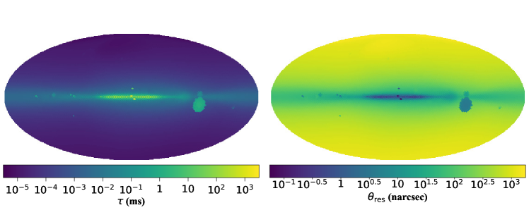
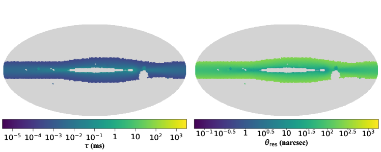
Figure 1: Top: The expected scattering timescale due to scattering in the Milky Way at 1.405 GHz from the NE2001 model of the electron distribution in the Milky Way (left) and the resolution of the Milky Way scattering screen assuming a distance to the screen of 1 kpc (right). Bottom: The same plot with regions masked for which the DSA-110 (with 250-MHz bandwidth) would be insensitive to galactic scintillation or $\gtrsim 1$ ms of extragalactic scattering. Note that the DSA-110 is best suited for detecting scintillation from Milky Way scattering screens with resolutions of 0.1 to 1 $\mu$as, and is not sensitive to scintillation along Milky Way sightlines with high scattering (such as towards the Galactic center) or with very low scattering (such as those at high Galactic latitudes).

When scintillation is observed that is consistent with our expectations for scattering in the Milky Way from the NE2001 model, the presence of scintillation indicates that the FRB is unresolved by the Galactic screen and we can constrain the angular broadening of any extragalactic scattering to be

$$\theta_{\mathrm{EG}}<\theta_{\mathrm{res,MW}}\;.$$ (45)

When scattering is observed, this angular limit can be combined with the scatter-broadening timescale, $\tau_{\mathrm{EG}}$, to place a limit on the separation between the scattering screen and the source:

$$d_{\mathrm{src}}-d_{\mathrm{EG}} <\frac{\theta_{\mathrm{res,MW}}^{2}d_{\mathrm{src}}d_{\mathrm{EG}}}{c\tau_{\mathrm{EG}}}(1+z_{\mathrm{EG}})\;,$$ (46)

where $z_{\mathrm{EG}}$ and $d_{\mathrm{EG}}$ are the redshift of and angular diameter distance to the extragalactic scattering screen. When the scattering is occurring close to the source, we can write:

$$d_{\mathrm{src}}-d_{\mathrm{EG}} <\frac{\theta_{\mathrm{res,MW}}^{2}d_{\mathrm{src}}^{2}}{c\tau_{\mathrm{EG}}}(1+z)$$ (47)

$$<32\,\mathrm{kpc}\left(\frac{\theta_{\mathrm{res,MW}}}{100\,\mathrm{nano-arcsec}}\right)^{2}\left(\frac{\tau_{\mathrm{EG}}}{1\,\mathrm{ms}}\right)^{-1}\left(\frac{d_{\mathrm{src}}}{1\,\mathrm{Gpc}}\right)^{2}\left(\frac{1+z_{\mathrm{EG}}}{1.325}\right)\;.$$ (48)

This argument has been used by Masui et al. (2015) to associate scattering and a high rotation measure to the host galaxy of FRB 110523 and by Farah et al. (2018) to place the material scattering FRB 170827 by 4.1 $\mu$s to within 60 Mpc of the source. We will adopt frequency-dependencies of the scattering timescales and broadening angles of $\tau_{\mathrm{EG}}\propto f_{\mathrm{obs}}^{-4.4}$ and $\theta_{\mathrm{res,MW}}\propto f_{\mathrm{obs}}^{-1.2}$, so the critical lens-source distance that we are sensitive to, $d_{\mathrm{crit}}$, is $\propto f_{\mathrm{obs}}^{4.6}$ and there is a strong preference for observations at low frequencies. However, at very low frequencies scattering from within the Milky Way may mask any extragalactic scattering, limiting our ability to constrain the extragalactic scattering timescale.

For an unchanging scattering timescale with distance (i.e., ignoring any redshift-evolution of the turbulent properties of FRB host galaxies as well as the redshift dependence in equation (35)), the critical distance between the extragalactic lens and source for which the Milky Way scattering screen resolves the further scattering screen is $\propto d_{\mathrm{src}}^{2}(1+z_{\mathrm{EG}})$, assuming the extragalactic lens is close to the source. This is maximized (assuming cosmological parameters from Planck Collaboration et al. (2016), including $H_{0}=(67.8\pm 0.9)$ km s^-1 Mpc^-1 and $\Omega_{M}=0.308\pm 0.012$) at $z=3.8$, at which a Galactic screen resolution of $<44$ nano-arcseconds is needed to resolve a distance $d_{\mathrm{lens,src}}=50\,$kpc for an extragalactic scattering timescales of 1 ms. At redshifts below 0.2 (for which we can obtain detailed observations of the host galaxy to identify star-forming regions and the location of the FRB within the host), a Galactic screen resolution of $<190$ nano-arcseconds is required to resolve a screen-source separation of 50 kpc when $\tau=1\,$ms. To understand the prospects of multi-tracer studies of turbulence in FRB host galaxies with current and upcoming FRB surveys, we estimate the fraction of FRBs detected by these surveys at redshifts $<0.2$ and seen through parts of the Milky Way with sufficient angular resolution to resolve a 50 kpc lens-source distance. We focus on the DSA-110 FRB survey, which will enter a commissioning and early science phase in summer of 2021. In Appendix B, we present similar estimates for the current ASKAP CRAFTS survey as well as CHORD and DSA-2000, future instruments in their design phases. In all cases, we use frbpoppy (Gardenier, 2019) to estimate the redshift distribution of detected FRBs, as described in Appendix B.

We use the NE2001 model to obtain the resolution of the Galactic screen, and adopt a minimum declination of $-30$ deg for the DSA-110. We find that 1.2% and 17.4% of the sky visible to the DSA-110 has sufficient resolution to be sensitive to a screen-source separation of 50 kpc at all redshifts and at $z\leq 0.2$, respectively, for a FRB with 1-ms scattering at 1.405 GHz. If the FRB population traces stellar mass density in the Universe, then approximately 1 in 4 of FRBs detected by the DSA-110 will be at $z<0.2$. If the DSA-110 spends equal time searching all areas of the sky, then approximately 1 in 24 of DSA-110 FRBs will meet these conditions (low redshift, viewed through a sufficiently-resolving part of the Milky Way) to undertake an in-depth study of turbulence and scattering in the host galaxy as described here. The final number of DSA-110 sources for which this study can be done also depends on the distribution of scattering in host galaxies, which we do not attempt to model here.

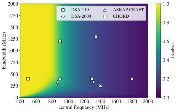
Figure 2: The fraction of sightlines through the galaxy for which a 50-kpc source-screen distance could be resolved, as a function of central observing frequency and observing bandwidth. We have adopted a fiducial scattering timescale for scattering in the host galaxy of 1 ms at 1.405 GHz, and assume that the timescales for both extragalactic scattering and scattering in the Milky Way (calculated using the NE2001 model at 1 GHz) are presumed to scale as $f_{\mathrm{obs}}^{-4.4}$. The DSA-110 survey, with a central frequency of 1.405 GHz and a bandwidth of 250 MHz is indicated by the white x. In Appendix B, we also consider the coherent-search mode of the ASKAP CRAFT survey (triangles), the DSA-2000 (circles) and CHORD (squares). For each of these, we consider different central frequencies and bandwidths within the instrument’s capabilities.

In Fig. 2, we show how the fraction of the sky for which the Milky Way has sufficient resolution changes with central frequency and bandwidth of the instrument. We clearly see two effects: an increased bandwidth and lower central frequency (Galactic scintillation bandwidths are narrower at lower frequencies) allow detection of Galactic scintillation over a larger part of the sky, increasing the likelihood of observing an FRB for which we can localize the extragalactic scattering material using a two-screen model; and at lower frequencies the required resolution of the galactic screen decreases due to the increased fiducial scattering timescale (and broadening angle) at the extragalactic screen. The required resolution scales as $f_{\mathrm{obs}}^{-2.2}$ (assuming $\tau_{\mathrm{EG}}\propto f_{\mathrm{obs}}^{-4.4}$), while the resolution of the Galactic scattering screen scales as $f_{\mathrm{obs}}^{-1.2}$ (again, we assume $\tau_{\mathrm{MW}}\propto f_{\mathrm{obs}}^{-4.4}$), so that at lower frequencies the required resolution is met over more of the sky.

In all cases, we consider FRBs that are scattered to $>1$ ms at 1.405 GHz (the center frequency of the DSA-110 survey), and scale this scattering with $\tau\propto f_{\mathrm{obs}}^{-4.4}$. At the lowest frequencies, this results in scattering timescales $\sim 100$ ms. Recent results from the CHIME/FRB collaboration suggest that there may be a substantial undetected population of highly-scattered FRBs, but that their current detection pipeline is biased against events with scattering timescales above 10 ms (The CHIME/FRB Collaboration et al., 2021). Searching for FRBs with large scattering timescales is computationally challenging with current standard single-pulse search algorithms, but further development of search algorithms, including image-based searches, may enable discoveries of FRBs with high scattering timescales.

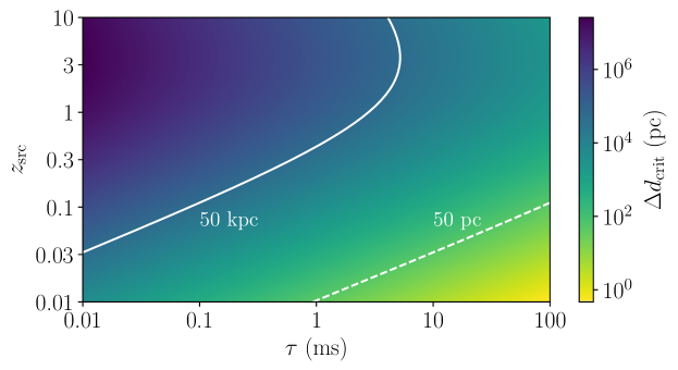
Figure 3: The critical source-screen separation, $\Delta d_{\mathrm{crit}}$, below which scintillation due to Galactic scattering with a resolution of 100 nano-arcseconds will resolve the scattering disk on the extragalactic screen, derived for sources at a cosmological redshift $z_{\mathrm{src}}$ with an extragalactic scattering delay of $\tau$. The white solid contour labels the critical distance of 50 kpc, for which extragalactic scattering could reasonably be associated with the host galaxy, while the white dashed contour labels a critical distance of 50 pc.

One will also encounter cases where no scintillation is observed from the Milky Way. Depending on the uncertainty in NE2001 expectations along the sightline (which might be somewhat assuaged by proximity to nearby pulsars), one may be able to place a lower limit on the angular scatter-broadening in these cases. The lack of scintillation where expected indicates that the burst is sufficiently angular-broadened by extragalactic scattering to be resolved by the Galactic screen. When combined with an observed temporal broadening timescale, this can allow one to rule out scattering within the host galaxy of the FRB. However, one must diligently confirm the properties of Galactic scattering towards the FRB in these cases, as some sightline-to-sightline or temporal variations in scattering (for example, extreme scattering events) are not captured in the NE2001 model.

Additional potential scattering locations include the IGM and the CGM of intervening galaxies. Studies of FRB scattering at these locations hold promise for furthering our understanding of the baryon content and distribution in the IGM and CGM (Macquart & Koay, 2013). Recently, scattering theory has been applied to FRB observations to constrain the distribution of cold gas in the halos of intervening galaxies (Prochaska et al., 2019; Cho et al., 2020) and turbulence in the ionized IGM (Ravi et al., 2016). Statistical studies of FRB DMs will likely also prove fruitful for revealing the structure of the IGM (e.g. Macquart & Ekers, 2018; Macquart et al., 2020; Xu & Zhang, 2020), including, for example, constraining the era of helium reionization (e.g. Caleb et al., 2019). In this paper, however, we focus specifically on scattering in the ISM of FRB host galaxies.

4 Case studies

Table 1: Constraints from radio and optical observations used to infer the turbulent properties of the host galaxies and host star-forming regions (SRs) of repeating FRBs. The SMs, and some EMs, are derived in this work.

	FRB 20190608B	FRB 20180916B	FRB 20121102A
Radio constraints
$\tau$ (ms)	3.3$\pm$0.2a	$<$1.6d	$<$9.6f
$f_{\mathrm{obs}}$ (MHz)	1200a	350d	500
$z$	0.1178b	0.0337$\pm$0.002e	0.19273$\pm$0.00008g
$\mathrm{SM}$ (kpc m-20/3)	240$\pm$130	$<$0.7	$<(1.0\pm 0.5)\times 10^{5}$
Optical constraints on associated star-forming regions
H${\rm\alpha}$ flux ($10^{-16}$ erg cm-2 s-1)	–	1.002$\pm$0.008e	2.6
Size of SR (pc)	640$\pm$320c	190h	1320
$\sigma_{v}$	15$\pm$0.55 km s-1 c	$290\pm 50$ km s-1	91.8$\pm$1.6 km s-1
EM (pc cm-6)	222$\pm$12c	310$\pm$140	510$\pm$160
Assumptions
$d_{\mathrm{lens,src}}$ (pc)	90$\pm$50	100$\pm$50	660$\pm$330
$l_{o}$ (pc)	150	150	1320

Table 2: Turbulent energy inferred from measurements of FRB scattering and optical line widths, along with estimates of the scale probed by each method.

	From scattering		From line widths
	Scale probed (m)	Energy (erg $M_{\odot}^{-1}$)	Scale probed (m)	Energy (erg $M_{\odot}^{-1}$)
FRB 20190608B	$3.3\times 10^{8}$	$3.3\times 10^{49}$ to $2.0\times 10^{51}$	4.6$\times 10^{18}$	$2.2\times 10^{45}$
FRB 20180916B	5.5$\times 10^{8}$	$<4\times 10^{48}$	4.5$\times 10^{18}$	$8\pm 3\times 10^{47}$
FRB 20121102A	1.3$\times 10^{9}$	$<3\times 10^{49}$	$4\times 10^{19}$	8.4$\pm 0.3\times 10^{46}$

We will focus on three FRBs that have been localized to H$\alpha$-emitting regions within their host galaxies: FRB 20121102A (Bassa et al., 2017), FRB 20180916B (Marcote et al., 2020), and FRB 20190608B (Chittidi et al., 2020). Of these three sources, only FRB 20190608B exhibits temporal scattering inconsistent with expectations from the Milky Way (Day et al., 2020); both FRB 20121102A (Josephy et al., 2019) and FRB 20180916B (Chawla et al., 2020) have stringent upper limits on their extragalactic scattering timescales. For all three sources, optical imaging and spectroscopic observations have been used to characterize the host galaxies and FRB-source local environments. Here, we consider these three sources in turn, and compare their observed scattering (or scattering limits) to constraints on the local environment from optical observations. Table 1 lists relevant constraints from both optical host-galaxy follow-up and radio FRB observations, as well as assumptions on the scattering geometry and the scales in the turbulent media.

We will assume, for the H$\alpha$-emitting gas in all three host galaxies, a temperature of $10^{4}$ K with a sound speed of 10 km s^-1, and turbulence that follows a Kolmogorov spectrum with $\beta=11/3$ and an inner scale of 1000 km, consistent with Cordes et al. (2016). We note that the inner scale is poorly constrained even in the Milky Way. The multi-tracer analysis of Armstrong et al. (1995), which probes down to scales of $\sim 10^{7}$ m, is consistent with an inner scale $\lesssim 10^{8}$ m. Detailed pulsar scattering (Rickett et al., 2009) studies and interferometric studies of anglar broadening and image wander (Spangler & Gwinn, 1990) suggest the inner scale may be $\sim 100$ km. However, as discussed in Section 1, evidence that localized, anisotropic scattering may dominate pulsar scintillation (e.g. Putney & Stinebring, 2006; Brisken et al., 2010) raises doubt that the plasma at tiny scales probed by pulsars is indeed part of the same isotropic turbulent cascade seen at larger scales. To obtain physical scales at the host galaxies from angular ones, we use cosmological parameters from (Planck Collaboration et al., 2016).

In Fig. 4, we compare the power on the outer and Fresnel scales measured from the burst scattering timescales and emission line widths for these three FRBs and their local environments to the “power law in the sky” in the Milky Way. We note two major differences between studies in the Milky Way and our study: in the Milky Way, tracers are present at intermediate scales that aren’t probed in our study of FRB host galaxies; and in the Milky Way tracers are typically averaged over multiple sightlines and different tracers can be acquired for different sightlines. In this study, we are considering two tracers that probe approximately the same region of the FRB host galaxy.

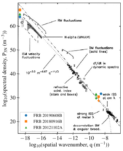
Figure 4: The “power law in the sky” measured in the Milky Way reproduced from Chepurnov & Lazarian (2010) and including the original data of Armstrong et al. (1995) (black and white) with points from this study of extragalactic galaxies with FRB scattering and H$\alpha$ line widths over plotted in color. Blue circles, orange squares, and green triangles show results for the host galaxies of FRB 20190608B, FRB 20180916B and FRB 20121102A respectively. Points at large $q$ (right hand of the plot) are from scattering measurements, while points at low $q$ (left hand of the plot) are from non-thermal velocity dispersions measured from H$\alpha$ line widths. Note that for consistency with Armstrong et al. (1995), we adopt a definition of the spatial wavenumber $q=1/l$ in this figure. Where the points are not upper limits, errorbars are shown that represent uncertainties determined from the assumed uncertainty on the lens-source screen distance and the measured uncertainties on the SM, non-thermal velocity dispersion and electron density. These error bars do not include uncertainty in the electron density, sound speed of the gas, outer scale, or the spectral index of the turbulent cascade, all of which should ultimately be considered.

4.1 FRB 20190608B

FRB 20190608B was discovered and localized by the Australian Square Kilometer Array Pathfinder (ASKAP) (Macquart et al., 2020) and associated with a host galaxy at redshift $z=0.1178$. The host galaxy is a spiral galaxy with stellar mass $M_{\star}\approx 10^{10.4}M_{\odot}$ and star formation rate $\mathrm{SFR}\approx 1.2M_{\odot}\,\mathrm{yr}^{-1}$ (Bhandari et al., 2020). High time-resolution analysis of the radio burst yields a scattering timescale of $\tau=3.3\pm 0.2$ ms at a frequency of 1.28 GHz (Day et al., 2020), significantly longer than expected from scattering in the Milky Way (34 ns according to the NE2001 model). Day et al. (2020) also measure the spectral index of the scattering timescale, and find $\tau\propto f_{\mathrm{obs}}^{-\alpha}$, where $\alpha=3.5\pm 0.9$.

Here we assume that the scattering observed in FRB 20190608B originates in its host galaxy. A detailed analysis of the foreground environment by Simha et al. (2020) finds no foreground galaxy within 2.5 Mpc in the SDSS catalogue, as well as no foreground galaxy in the 1 arcmin Keck Cosmic Web Imager (KCWI) field used to study the local environment of FRB 20190608B. They simulate the cosmic web using SDSS galaxies within 400 arcminutes of the line-of-sight to the host galaxy of FRB 20190608B and find it implausible that the foreground is responsible for the temporal scattering of the FRB. Day et al. (2020) observe structure in the spectrum of FRB 20190608B that may be Galactic scintillation, but for which they are unable to measure a decorrelation bandwidth. A screen in the Milky Way with the NE2001 scintillation bandwidth of 5.4 GHz at 1200 MHz has a resolution of only 2 $\mu$as, and a confirmation of scintillation in the Milky Way would allow a localization of the extragalactic scattering material to within 320 kpc of the source. While we cannot claim that the scattering definitively originates in the host galaxy, we will continue with this case study to demonstrate the power of our analysis framework.

Chittidi et al. (2020) examine the local environment of FRB 20190608B in detail using HST WFC3/UVIS imaging and Keck/KCWI integral field spectroscopy. The HST images revealed that the positional localization of FRB 20190608B coincides with a knot of star formation in one of the spiral arms of the host galaxy. While they do not observe the H${\rm\alpha}$ line with KCWI, they infer the H${\rm\alpha}$ flux of the star-forming knot from the H${\rm\beta}$ flux, assuming the flux ratio follows expectations for HII regions, and calculate $\mathrm{EM}=222\pm 12$ pc cm^-6. In the KCWI H${\rm\beta}$ maps, Chittidi et al. (2020) measure a velocity dispersion of $\sigma_{v}=15\pm 0.55$ km s^-1 within a region including both the burst localization and the star-forming knot.

In the following, we derive properties of the ISM local to the source of FRB 20190608B from the optical data in hand. We subtract a thermal width of $\sigma_{t}=9.1\pm 2.7$ km s^-1 (Osterbrock & Ferland, 2006) (corresponding to a temperature of $(1.0\pm 0.5)\times 10^{4}$K) from the velocity dispersion in quadrature to find a non-thermal velocity dispersion of $\sigma_{nt}=11.9\pm 2.8$ km s^-1. We ignore the natural broadening of the line, which is three orders of magnitude smaller than the thermal broadening. We estimate the size of the star-forming region to be $\approx 1\pm 0.5$ spaxel in the KCWI images, or $640\pm 320$ pc at an angular diameter distance of 453 Mpc. As the host galaxy is face-on (Chittidi et al. (2020) measure an inclination angle of $37\pm 3\,\deg$), if this region were spherical it would extend above the thin disk of the galaxy, which Chittidi et al. (2020) take to be $\sim 150$ pc. We estimate the line-of-sight extent to be $\sim 150\,\mathrm{pc}\,\cos^{-1}(37\,\deg)$, and take $L=190\pm 90\,\mathrm{pc}$. We adopt the scale height as the outer scale, $l_{o}=150\,\mathrm{pc}$. From the EM and the line-of-sight extent of the region, we infer an electron density between 0.08 and 0.85 cm^-3, assuming a filling fraction between 0.1 and 1, $\zeta=2$ and $\epsilon=1$. This would contribute a DM to FRB 20190608B in the observer frame of $\sim 10-140$ pc cm^-3, consistent with the total host contribution of $137\pm 43$ pc cm^-3 (Chittidi et al., 2020).

The radio observations of FRB 20190608B can be used to predict the non-thermal velocity dispersion in the ionized gas, assuming a Kolmogorov turbulent fluctuation spectrum, using equation (24). In addition to measurements of the SM, EM, and outer scale, equation (24) requires estimates of the sound speed, clumpiness of the ionized gas (given by $f_{f}$, $\epsilon$ and $\xi$), and the path length of the FRB through the gas. We will adopt our fiducial values of $\zeta=2$ and $\epsilon=1$. As shown in equations (7) and (8), the observed scattering time $\tau$ is related to the SM through the diffractive scale, $r_{\mathrm{diff}}$, the characteristic size of fluctuations on the scattering screen. For FRB 20190608B, and assuming a screen-source distance $d_{\mathrm{lens,src}}=90\pm 50$, $r_{\mathrm{diff}}=6.0\pm 1.6\times 10^{6}$ cm and $\mathrm{SM}=240\pm 120\,\mathrm{kpc}\,\mathrm{m}^{-20/3}$. The scattering probes fluctuations at the Fresnel scale, equation (9), $\sim 3\times 10^{8}$ m.

For $f_{r}=1$ and $f_{f}=0.1$, we calculate from the radio observations an expected velocity dispersion of $(8.2\pm 2.1)\times 10^{4}$ km s^-1, many orders of magnitude larger than the observed value of $11.9\pm 2.8$ km s^-1. Varying $f_{r}$ between 0.5 and 1, and $f_{f}$ between 0.1 and 1, we find a range for the velocity dispersion of $1.9-14.6\times 10^{4}$ km s^-1. The energies calculated from the radio scattering observations and the observed velocity dispersion from H${\rm\beta}$ KCWI maps (calculated from equations (32) and (34)) are given in Table 2. The energy from the optical line width is a few orders of magnitude smaller than the energy inferred from the scattering timescale, assuming that both of these are probing the same turbulent fluctuation spectrum within the H$\alpha$ region.

As the energies are separated by only a couple of orders of magnitude, we can attempt to reconcile them by varying the inner and outer scales. An outer scale six orders of magnitude smaller than our adopted value (i.e., $l_{o}\sim 30$ AU) is needed to reconcile the two energies, holding the inner scale at 1000 km. It is difficult to motivate energy injection on such a small scale, and therefore such a small outer scale seems unlikely. From equations (32) and (6) we see that $E\propto l_{i}^{1/3}$; however, this applies only when the inner scale is larger than the diffractive scale (see (6)), which, from the scattering timescale of FRB 20190608B, we calculate to be $6.0\pm 1.6\,\times\,10^{6}$ cm. Varying the inner scale can only decrease the energy by a factor of $\sim 10$ due to this flattening in the SM function against the inner scale. Alternatively, the electron density ($E\propto n_{e}^{-2}$, see equation (32)) would need to be 70 times larger, for which the region would contribute a DM between 440 and 9960 pc cm^-3, much larger than the estimated host DM and even exceeding the total DM of $338.7\pm 0.5$ pc cm^-3 (Macquart et al., 2020).

A final point of uncertainty is the scaling of the power spectrum over the orders of magnitude that separate the scales probed by these two tracers. We have assumed a Kolmogorov scaling, $\beta=11/3\approx 3.7$, but with a slightly shallower power law, $\beta\sim 3.2$ the energies probed by FRB scattering (at $3.3\times 10^{8}$ m) and the H${\rm\beta}$ velocity dispersion (at $4.6\times 10^{18}$ m) are consistent. While this is a small change in the power-law index, the energy difference at small scales is $10^{5}$ larger than what one would extrapolate from the velocity dispersion measurement assuming $\beta=11/3$. Alternatively, this large excess power on small scales could be due to a break or bump in the power spectrum. Indeed, this is put forth by Johnson et al. (2018) as an explanation for the increased power on small scales in the fluctuation spectrum towards the Milky Way Galactic Center. For isotropic turbulence, the scattering index $\alpha$ measured by Day et al. (2020) corresponds to a power-law index $\beta=2\alpha(\alpha-2)^{-1}$ of $\beta=4.7\pm 1.6$, consistent with the $\beta\sim 3.2$ power-law index inferred from comparing fluctuations on large and small scales and suggesting that the scattering index may be constant across the intermediate scales. To distinguish between these cases, additional tracers of the fluctuation spectrum or the power law index are necessary.

4.2 FRB 20180916B

FRB 20180916B is a repeating source discovered by the CHIME/FRB Collaboration (CHIME/FRB Collaboration et al., 2019b) and localized to an emission region in a massive spiral galaxy at redshift $z=0.0337\pm 0.002$ (Marcote et al., 2020). FRB 20180916B is also the first FRB to be detected below $400$ MHz (Chawla et al., 2020; Pilia et al., 2020); this low-frequency detection provides a stringent upper limit on the extragalactic scattering timescale of $<1.6$ ms at $350$ MHz (Chawla et al., 2020). Recently, a detection of FRB 20180916B with LOFAR at 110 to 188 MHz (Pastor-Marazuela et al., 2020; Pleunis et al., 2020) shows a scattering tail with $\tau\sim 50$ ms at 150 MHz, consistent with the upper limit set by (Chawla et al., 2020) and with expectations for galactic scattering from the NE2001 model. Any scattering in the host galaxy must be below this level to be obscured by scattering in the Milky Way.

As in the previous case study, we will start by deriving properties of the ISM local to the source of FRB 20180916B from optical observations of the host galaxy. Marcote et al. (2020) estimate the projected size of the emission region to be $1.5$ kpc². In a region of $1.5\times 2$ arcsec² surrounding the FRB localization, Marcote et al. (2020) measure an extinction-corrected H${\rm\alpha}$ luminosity of $L_{\mathrm{H}\alpha}\sim(2.0\pm 0.1)\times 10^{39}\,\mathrm{erg}\,\mathrm{s}^{-1}$, which they suggest is dominated by the star-forming clump. The H${\rm\alpha}$ line at the location of the FRB is measured by Marcote et al. (2020) to have a centroid and width of 6787.5 Å and 6.5 Å respectively. We will adopt the calibration precision of 0.8 Å as the uncertainty on both the line centroid and width. Estimating the thermal velocity dispersion as $9.1\pm 2.7$ km s^-1, we calculate a non-thermal velocity dispersion of $290\pm 50$ km s^-1 from the H${\rm\alpha}$ line width measured by Marcote et al. (2020).

Through detailed HST observations, Tendulkar et al. (2020) found that this V-shaped emission region is composed of many clumps. The one closest in projected distance from FRB 20180916B is at the vertex of the V, with a H${\rm\alpha}$ luminosity of $9\times 10^{37}$ erg s^-1 (detected after smoothing the original 30 mas HST WFC3/F673N emission maps with a Gaussian kernel with FWHM 294 mas; we take 20% uncertainty on this measurement). Tendulkar et al. (2020) measure a projected distance between this star-forming region, which has a size of 270 mas or 190 pc, and FRB 20180916B of 250$\pm$190 pc. We will adopt a path length through the region of $L=190\pm 100$ pc. We estimate the EM from the H${\rm\alpha}$ luminosity of the region according to equation (3) of Tendulkar et al. (2017) (see also Reynolds (1977)),

$$\mathrm{EM}(\mathrm{H}\alpha)=2.75\,\mathrm{pc}\,\mathrm{cm}^{-6}T_{4}^{0.9}\left(\frac{S(\mathrm{H}\alpha)_{s}}{\mathrm{Rayleigh}}\right)\,$$ (49)

where $S(\mathrm{H}\alpha)_{s}$ is the H${\rm\alpha}$ surface density given in the source frame,

$$S(\mathrm{H}\alpha)_{s}=(1+z)^{4}\frac{F_{\mathrm{H}\alpha}}{\pi ab}\;.$$ (50)

$F_{\mathrm{H}\alpha}$ is the H${\rm\alpha}$ flux, and $a$ and $b$ are the semi-major and semi-minor axes respectively. For FRB 20180916B, we find $\mathrm{EM}=310\pm 140\,\mathrm{pc}\,\mathrm{cm}^{-6}$. This corresponds to electron densities of 0.2$\pm$0.10 and 0.6$\pm$0.3 cm^-3 for filling factors of 0.1 and 1 (assuming $\zeta=2$ and $\epsilon=1$), and this region would contribute a DM in the observer frame between 10 and 170 to the FRB. This is consistent with the host DM limit of $<70$ for FRB 20180916B (Marcote et al., 2020).

In the absence of any observed extragalactic scattering towards FRB 20180916B, we will use the scattering upper limit of $\tau<1.6$ ms at 350 MHz (Chawla et al., 2020) to place an upper limit on the non-thermal velocity dispersion in the ISM local to FRB 20180916B predicted from radio-wave scattering. Assuming a distance between the lens and the FRB source of $d_{\mathrm{lens,src}}=100\pm 50$ pc, we find $r_{\mathrm{diff}}>3.2\times 10^{7}$ cm and $\mathrm{SM}<0.8\,\mathrm{kpc}\,\mathrm{m}^{-20/3}$. From the SM and EM, we calculate an expected non-thermal velocity dispersion of $<480$ km s^-1 for $f_{f}=0.1$ and $f_{r}=1$. Varying $f_{f}$ between 0.1 and 1, and $f_{r}$ between 0.5 and 1, we predict $\sigma_{v}<620$ km s^-1, similar to the velocity dispersion of $290\pm 50$ km s^-1 calculated from the observed H${\rm\alpha}$ line width. The energy in turbulence corresponding to both the constraint on scattering from the burst observations and the optical velocity dispersion are listed in Table 2. In this case, the limit from scattering is consistent with the H${\rm\alpha}$ line width measured at the location of the FRB by Marcote et al. (2020).

4.3 FRB 20121102A

FRB 20121102A was the first FRB to be observed to repeat (Spitler et al., 2016) and the first to be localized and associated with a host galaxy (Chatterjee et al., 2017). The host galaxy of FRB 20121102A is a star-forming dwarf galaxy at a redshift $z=0.19273(8)$ (Tendulkar et al., 2017). VLBI observations revealed a persistent radio source close to the FRB position (Marcote et al., 2017). High-resolution observations of the host galaxy reveal a star-forming region that encompasses both the FRB location and the associated persistent radio source (Kokubo et al., 2017; Bassa et al., 2017).

Again, we start by extracting properties of the ISM local to the FRB source from optical observations. Bassa et al. (2017) measure the projected half-light radius of the star-forming region in the F101W filter of their HST observations to be $0.20\pm 0.01$ arcsecond, giving a diameter of the star-forming region of $1.32\pm 0.07$ kpc (using an angular diameter distance of $682.2\pm 0.2$ Mpc). This is consistent with the upper limit on the FWHM of the H${\rm\alpha}$-emitting region, $<0.57$ arcsecond, placed by Kokubo et al. (2017) using Subaru/Kyoto H${\rm\alpha}$ images. Within the star forming region, Kokubo et al. (2017) measure an H${\rm\alpha}$ flux consistent with that reported by Tendulkar et al. (2017) for the entire galaxy, indicating that the H${\rm\alpha}$ flux measured by Tendulkar et al. (2017), $2.6\times 10^{-16}\,\mathrm{erg}\,\mathrm{cm}^{-2}\,\mathrm{s}^{-1}$, is dominated by the star-forming region. From the H${\rm\alpha}$ flux from Tendulkar et al. (2017) and the area of the star-forming region measured by Bassa et al. (2017), we calculate $\mathrm{EM}=510\pm 160$ pc cm^-6. Assuming a path length through the region equal to the region’s diameter, this corresponds to an electron density of $0.097\pm 0.016$ or $0.31\pm 0.05$ cm^-3 for filling factors of 0.1 or 1 (assuming $\zeta=2$ and $\epsilon=1$). If the FRB path length through the region is equivalent to the half-light radius of the region, this would contribute a DM between 50 and 400 to the FRB, consistent with the analysis of Tendulkar et al. (2017) based on the H$\alpha$ emission of the host galaxy and the 340 pc cm^-3 extragalactic (IGM + host galaxy + local environment, Tendulkar et al., 2017) DM of FRB 20121102A. Tendulkar et al. (2017) measure a width of the H${\rm\alpha}$ line of $2.02\pm 0.03$ Å. From this width, we measure a velocity dispersion in the star-forming region of $92.2\pm 1.4$ km s^-1. Subtracting a thermal contribution of $9.1\pm 2.7$ km s^-1 in quadrature, we estimate a non-thermal velocity dispersion of $91.7\pm 1.6$ km s^-1.

As was the case for FRB 20180916B, there is no evidence of extragalactic scattering towards FRB 20121102A from radio observations, but we can still place an upper limit on the scattering measure and the predicted non-thermal velocity dispersion in the local ISM. The best constraints on scattering of FRB 20121102A come from observations with the CHIME/FRB instrument, which yield an upper limit on the scattering timescale of 9.6 ms at 500 MHz (Josephy et al., 2019). Assuming the source and scattering screen are separated by a distance $d_{\mathrm{lens,src}}=(0.5\pm 0.25)\,\mathrm{FWHM}_{\mathrm{SFR}}$, we limit the diffractive scale and the SM to be $r_{\mathrm{diff}}>2.9\times 10^{7}$ cm and $\mathrm{SM}<4.3$ kpc m^-20/3.

Combining the scattering and emission measures, we find, for $f_{r}=1$ and $f_{f}=0.1$, an expected velocity dispersion of $\sigma_{v}<1100$ km s^-1. For $f_{R}=0.5$ and $f_{f}=0.1$, $\sigma_{v}<1600$ km s^-1. This constraint is consistent with the optical measurement of $91.7\pm 1.6$ km s^-1, but the SM is sensitive to only much larger velocity dispersions than that measured from the emission line width. This suggests that, for FRB 20121102A, current radio burst observations do not provide strong constraints on the turbulence in the plasma. A burst detection at lower frequency, where radio-wave scattering is stronger, may provide a stronger constraint. However, Spitler et al. (2018) measure, at 5 GHz, a scintillation bandwidth of $6.4\pm 1.6$ MHz consistent with expectations of Galactic scattering. At 300 MHz, this will result in a scattering timescale of $\sim 4$ ms, which would mask extragalactic scattering below this level. The energies calculated from both the velocity dispersion constraint from scattering and the non-thermal velocity dispersion calculated from the H${\rm\alpha}$ line width are shown in Table 2.

With only an upper limit on the SM, we can still place a lower limit on the outer scale if we assert that the scattering is probing the same turbulent cascade as the gas seen in emission and the scales probed by radio-wave scattering and the H${\rm\alpha}$ line width are connected by a Kolmogorov turbulence power spectrum. In this case, we find $l_{o}>4.4\times 10^{15}$ m ($>0.014\,$pc), consistent with our expectations of an outer scale on the order to $100\,$pc (approximately the size of the star-forming region).

5 Discussion and Conclusions

5.1 Summary of results

In this work:

1. We have presented a formalism for combining FRB SMs with optical followup of FRB host galaxies to trace density and velocity fluctuations in the ISM of these host galaxies on multiple scales. As a method of comparison, we use the turbulent energy inferred from these observables. The turbulent energy is related to the SM (sensitive to density fluctuations on the Fresnel scale, $\sim 10^{8}$ m) and non-thermal velocity dispersion (sensitive to velocity fluctuations on the outer scale, $\sim 10^{18}$ m) by equations (32) and (34) respectively. By inferring the turbulent energy on these vastly different scales, we can constrain the nature of the turbulent cascade in the ISM of galaxies besides the Milky Way, allowing us to study multiple instances of density-fluctuation spectra. At the same time, this methodology provides insight into the local environments of FRB sources and the origin of the observed scattering.

2. We have shown that upcoming FRB surveys will be able to use the presence of Galactic scintillation to determine the location of FRB scattering screens. For example, over $>15\,\%$ of the visible sky, the DSA-110 will be able to determine whether extragalactic scattering is originating from within 50 kpc of the FRB source of $z\leq 0.2$ FRBs scattered on 1 ms timescales at 1.405 GHz. Surveys at lower frequencies and with wider bandwidths will be able to make this determination over a much larger part of the sky; for example $>99\,\%$ of the sky for a CHORD observation of a similarly scattered FRB between 300 and 700 MHz.

3. We have presented three case studies to demonstrate the power of this technique. In all cases, we compare measurements or limits on extragalactic scattering to properties of HII regions near the FRB sources in their host galaxies.

   1. FRB 20190608B, with an extragalactic scattering timescale of $3.3\pm 0.2$ ms at 1200 MHz that most likely originates from the host galaxy or source local environment (Chittidi et al., 2020) although a search for Galactic scintillation was inconclusive (Day et al., 2020). From the scattering timescale, we infer a turbulent velocity dispersion $\sim 4$ orders of magnitude higher than that measured from the H${\rm\beta}$ line width. Such a large discrepancy cannot be explained by varying the outer and inner scales, but a decrease in the index of the density fluctuation power spectrum to $\beta\sim 3.2$ can reconcile this difference.

   2. FRB 20180916B, with a limit on extragalactic scattering of $>1.6\,$ms at 350 MHz, set by Galactic scattering towards FRB 20180916B. The upper limit on the turbulent energy inferred from the scattering timescale is approximately twice the measurement from the H${\rm\alpha}$ line width. These measurements are consistent with a Kolmogorov turbulent cascade over the ten orders of magnitude between the scales probed by the two processes.

   3. FRB 20121102A, with a limit on the extragalactic scattering of $<9.6\,$ms at 500 MHz. The upper limit on the turbulent energy inferred from the scattering timescale is more than two orders of magnitude larger than the measurement from the H${\rm\alpha}$ line width, suggesting that the scattering timescale constraints are insufficient for this type of study in FRB 20121102A.

5.2 Improving constraints on the density fluctuation power-spectrum

The energy derived from the scattering timescale (equation (26)) depends strongly on the form of the turbulent power spectrum that we assume, including the power-law index, the inner scale ($E\propto l_{i}^{1/3}$ for Kolmogorov turbulence), and the outer scale ($E\propto l_{o}^{2/3}$, which we associate with the size of the nearby star-forming regions in our case studies), as well as properties of the scattering medium, including the electron density ($E\propto\langle n_{e}\rangle^{2}$, which we have constrained through the EM) and the line-of-sight separation between the source and the scattering material. We also note that we have considered solely isotropic turbulence in this work; anisotropic turbulence could also be considered with modification of the relations between the observables (scattering timescale and non-thermal velocity dispersion) and the amplitude of the density and velocity fluctuations.

There are a number of factors here that can be better constrained. To determine the EM of the H$\alpha$-emitting regions from the H$\alpha$ flux (and derive their electron densities), we need their spatial sizes. Strong constraints on these sizes from high-spatial resolution optical observations of FRB host galaxies are therefore important for constraining the electron density.

The properties of the H$\alpha$-emitting gas can also be probed directly from the observed emission lines. High-resolution spectral line observations are critical to constraining the properties of this gas. In particular, the SII (6716 Å or 6731 Å) to H$\alpha$ line-width ratio provides a direct decomposition of the thermal and non-thermal components to the velocity, due to the high mass ratio of these two elements (32 to 1) (e.g. Reynolds, 1985). The SII to H$\alpha$ line flux ratio is also a useful diagnostic of gas conditions, including the ionization state. The electron densities of $\sim 0.1$ cm^-3 inferred from the EMs in Section 4, the high SII 6716 Å to H$\alpha$ flux ratio of $0.24\pm 0.07$ in the local environment of FRB 20180916B (Marcote et al., 2020), and the non-detection of a point source of H$\alpha$ emission near FRB 20180916B (Tendulkar et al., 2020) all suggest that the H$\alpha$ emission in the local environment of FRB 20180916B is dominated by diffuse ionized gas like the Milky Way WIM (diffuse ionized gas present throughout the Milky Way with temperatures $\sim$6000 to 10000 K and generally lower ionization states than classical HII regions), or the diffuse ionized gas (DIG) of extragalactic galaxies. A different picture emerges for FRB 20121102A; the low SII 6716 Å to H$\alpha$ line flux ratio (0.06$\pm$0.01 after correcting for extinction) observed by Tendulkar et al. (2017) from the host galaxy of FRB 20121102A is more consistent with an HII region than the Milky Way WIM. The flux ratio between the 6716 Å and 6731 Å components of the SII doublet can also be used to constrain the electron density independently when it is above 37 cm^-3 (Osterbrock & Ferland, 2006). The electron densities inferred from the EMs in our case studies are orders of magnitude below this value. The conclusion that the H$\alpha$ emitting gas in these regions of interest is too tenuous to measure the density using the SII line ratio is supported by the SII (6716 Å/6731 Å) line ratios for FRB 20121102A (1.7$\pm$0.5; spectra from (1.7$\pm$0.5, spectra from Tendulkar et al., 2017) and FRB 20180916B (2.0$\pm$0.3, spectra from Marcote et al., 2020), both larger than the $\lesssim 1.4$ ratio needed for measuring the electron density from the SII line ratio. These case studies show that high-spectral-resolution observations of the SII and H$\alpha$ emission lines is critical for studying the gas near an FRB source, and can probe the ionization state, temperature and density of the gas. This is especially powerful when combined with a size estimate of the H$\alpha$ emitting region from imaging; the temperature and size of the H$\alpha$ region reduce the number of variable parameters when inferring the electron density from the H$\alpha$ flux.

Our results also depend on assumptions for the inner and outer scale, but, as we see in our study of FRB 20190608B, the most important uncertainty in the turbulent power spectrum is the scaling index $\beta$. Thus, one of the best ways to improve this comparison between density and velocity fluctuations on different scales is to add tracers that can constrain $\beta$. In the Milky Way, the fringe tilt in pulsar dynamic spectra, refractive scintillation, and dispersion measure (DM) fluctuations are used as probes of intermediate scales of $\sim 10^{10}$ to $10^{14}$ m. Refractive scintillation, variation in the apparent flux of a source due to changes in the angular broadening scale, is not a good tracer of FRB local environments; angular broadening due to scattering in plasma close to the source is suppressed compared to that due to scattering close to the observer, as discussed in Section 3.1. Yang & Zhang (2017) consider possible sources of DM variations in repeating FRB sources, and predict contributions of $\sim 2\times 10^{-5}$ pc cm^-3 yr^-1 due to turbulent fluctuations in interstellar plasma with density fluctuations of $\sim 0.1$ cm^-3 (similar to the densities inferred from the EMs of the three FRBs presented in Section 4, which range from $\sim 0.1$ to $\sim 0.9$ cm^-3 for filling factors between $0.1$ and $1$). This is on the order of the best constraints for pulsar DM variations (e.g. You et al., 2007). However, Yang & Zhang (2017) find that DM variations due to expansion of a supernova remnant or HII region, or the proper motion of the FRB source with respect to an HII region, are much larger and, if present, will mask any smaller contributions due to density fluctuations in the plasma. The complex spectrotemporal structure of fast radio bursts further complicates detecting small-scale DM variations. Typically, FRB DM uncertainties are on the order of $\sim 0.1$ pc cm^-3, although Nimmo et al. (2020) measure the DM of FRB 20180916B to 0.006 pc cm^-3 precision. The DM of FRB 20121102A does show variation over time (Hessels et al., 2019) but the fluctuations expected from density variations have not been observed; Hilmarsson et al. (2020) find a steady increase in the DM of FRB 20121102A over a period of two years. FRB 20180916B shows no noticeable DM variations (e.g. Pastor-Marazuela et al., 2020).

Dynamic spectra are difficult to construct for repeating FRBs due to their low duty cycles. As repeat bursts tend to be temporally clustered (Oppermann et al., 2018; The CHIME/FRB Collaboration et al., 2020), observations of repeating FRB sources with highly sensitive radio instruments, such as FAST, may provide sufficient temporal sampling to construct a dynamic spectrum. However, it is possible that much of the spectrotemporal structure, including the downward marching ‘sad trombone’ effect seen in repeating FRB dynamic spectra (Hessels et al., 2019) is intrinsic; this intrinsic structure must be disentangled from any propagation-induced scintillation to use the dynamic spectrum as a probe of local turbulence. As our understanding of intrinsic FRB spectral structure advances, dynamic spectra and DM variations of repeating FRB sources may prove valuable ways of studying FRB environments; however, these methods do not take full advantage of the capability of instruments like ASKAP, the DSA and CHORD to localize non-repeating sources of FRBs, which may be a distinct class from FRB repeaters.

Multiple tracers at similar scales can be used to constrain the index of the fluctuation power spectrum (even if only at one end of the spectrum), adding some confidence to an extrapolation over orders of magnitude. If some optical spectral lines are resolved, additional information on the turbulent velocity power spectrum is present in the shape of the spectral line. This arises from Doppler shifting of the line by the turbulent velocity fluctuations. Lazarian & Pogosyan (2000, 2004, 2006) have developed the formalism for relating the line profile to the turbulent power spectrum, and, using this technique, the power-law spectral index and the outer scale of turbulence in neutral hydrogen have been measured at high latitudes in the Milky Way (Chepurnov et al., 2010) and in the Small Magellanic Cloud (Chepurnov et al., 2015).

At the opposite end of the spectrum, pulsar scattering indices from multi-band or wide-band scattering timescale measurements can be used to constrain the index of the fluctuation power spectrum at small spatial scales. For isotropic turbulence following a power-law spectrum, $\tau\propto\nu^{-\alpha}$ where $\alpha=2\beta/(\beta-2)$; however low values of $\alpha$ can be inferred if anisotropic scattering is not properly modelled (Geyer et al., 2017; Oswald et al., 2021). Day et al. (2020) apply this technique to four FRBs discovered and localized by ASKAP, including FRB 20190608B, as discussed in Section 4.

FRBs present the only means of probing density fluctuations in extragalatic ISM on $\ll$pc scales. The techniques we have developed will enable the use of FRBs to compare density-fluctuation measurements on scales across the putative turbulent cascades, extending these studies beyond the Milky Way for the first time. These considerations are also central in addressing the complementary question of the origin of observed FRB scattering. Even within the Milky Way, the physical origins of interstellar scattering remain inscrutable to this day, as the phenomenology of scattering grows richer. As FRB samples expand and localization accuracies improve, we anticipate that some of the most exciting discoveries about plasma along FRB sightlines may be revealed by scattering measurements.

Appendix A Derivation of the scatter broadening angle on the extragalactic screen

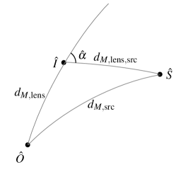
Figure 5: The comoving geometry. $d_{M,\mathrm{src}}$, $d_{M,\mathrm{lens}}$ and $d_{M,\mathrm{lens,src}}$ are the comoving distances between the observer and the source, the observer and the lens, and the lens and the source respectively. This figure is similar to Schneider et al. (1992), their Fig. 4.1, but specialized to a flat universe.

To derive the scattering broadening angle, $\theta_{\mathrm{scat}}$, for scattering at an extragalactic scattering screen, we work along the lines of Schneider et al. (1992, Chapter 4.6). For simplicity, we will assume a flat universe; Schneider et al. (1992) show that the same relation holds in a positively-curved universe. Our setup is shown in Fig. 5. We start with a transformation to comoving coordinates and conformal time, choosing a conformal factor at the observer of $a(z_{\mathrm{obs}})=1$, and write the geometric time delay imparted by lensing at a point $\hat{I}$ of radiation emitted by a point source at $\hat{S}$ as seen by an observer at $\hat{O}$.

$$c\Delta t_{\mathrm{geom}}=\Delta\eta_{\mathrm{geom}}=\frac{d_{M,\mathrm{lens,src}}d_{M,\mathrm{lens}}}{2d_{M,\mathrm{src}}}\hat{\alpha}^{2}\;.$$ (A1)

We use the relation between comoving distances ($d_{M}$) and angular diameter distance measured from $z_{1}$ to $z_{2}$ (for a flat universe),

$$d(z_{1},z_{2})=\frac{1}{1+z_{2}}(d_{M,2}-d_{M,1})\;,$$ (A2)

and write

$$c\Delta t_{\mathrm{geom}}=\frac{d_{\mathrm{lens,src}}d_{\mathrm{lens}}}{2\,d_{\mathrm{src}}}(1+z_{\mathrm{lens}})\hat{\alpha}^{2}\;.$$ (A3)

$t_{\mathrm{geom}}$ is the geometric time delay in conformal time. The geometric part of the phase difference is then

$$\Delta\phi_{\mathrm{geom}}=c\Delta t_{\mathrm{geom}}\Omega$$ (A4)

where $\Omega$ is the circular frequency in the conformal space. $\Omega$ is related to the frequency in the observer’s frame, $\omega$ by $\omega=a(z_{\mathrm{obs}})\Omega$. Our choice of conformal factor has thus ensured that $\omega=\Omega$, and we can write the phase imparted as

$$\Delta\phi_{\mathrm{geom}} =c\Delta t_{\mathrm{geom}}\frac{2\pi}{\lambda_{\mathrm{obs}}}$$ (A5)

$$=\frac{2\pi}{\lambda_{\mathrm{obs}}}\frac{d_{\mathrm{lens,src}}d_{\mathrm{lens}}}{2d_{\mathrm{src}}}(1+z_{d})\hat{\alpha}^{2};.$$ (A6)

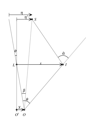
Figure 6: The lensing geometry. $\eta$, $x$ and $X$ are spatial coordinates on the source, lens, and observer planes respectively. $S$, $I$, and $O$ are the locations of the source, image, and observer, while $O^{\prime}$ and $L$ define our reference on all plane.

In this derivation, we have used a special reference line which intersects $\hat{O}$ and $\hat{I}$. We need to generalize this to any reference line, as shown in Fig.  6, to obtain the scattered wavefield at any point on the observer plane through the Fresnel-Kirchoff integral,

$$u(\mathbf{X}) =\frac{e^{-i\pi/2}}{2\pi r_{F}^{2}}\int d^{2}\mathbf{x}\exp\left[i\Delta\phi(\mathbf{x},\mathbf{X})\right]$$ (A7)

$$=\frac{e^{-i\pi/2}}{2\pi r_{F}^{2}}\int d^{2}\mathbf{x}\exp\left[\frac{2\pi}{\lambda_{\mathrm{obs}}}ic\tau(\mathbf{x},\mathbf{X})\right]\;,$$ (A8)

where $\tau(\mathbf{x},\mathbf{X})=\Delta t_{\mathrm{geom}}(\mathbf{x},\mathbf{X})+\frac{\phi(\mathbf{x})}{2\pi\nu}$. Here, $\mathbf{x}$, $\mathbf{X}$ and $\bm{\eta}$ are spatial coordinates at the lens, observer, and source planes, respectively, and $\phi(\mathbf{x})$ is the part of the phase independent of the observer position, which includes the phase imparted by the lens. The Fresnel scale, generalized to this cosmology, is given in equation (9). We will ignore the delay imparted by travel through the lens, assuming that its variation with $\mathbf{x}$ is much smaller than the variation of the geometric delay with $\mathbf{x}$.

As shown in Fig. 6, we have the following geometric relations:

$$\hat{\bm{\alpha}}d_{\mathrm{lens,src}} =(\bm{\theta}-\bm{\beta})d_{\mathrm{src}}\;,$$ (A9)

$$\bm{\eta} =\bm{\beta}d_{\mathrm{src}}\;,$$ (A10)

$$\bm{\eta}^{\prime} =\bm{\eta}-\bm{\phi}d_{\mathrm{lens,src}}\;,$$ (A11)

$$\mathbf{x} =\bm{\theta}d_{\mathrm{lens}}\;\mathrm{and}$$ (A12)

$$\mathbf{X} =\bm{\phi}d_{\mathrm{lens,obs}}=\bm{\phi}d_{\mathrm{lens}}(1+z_{\mathrm{lens}})\;.$$ (A13)

In the last line, we’ve used $d_{\mathrm{lens,obs}}$ to denote the angular diameter distance from the lens to the observer, and equation (A2) to write $d_{\mathrm{lens,obs}}=d_{\mathrm{obs,lens}}\frac{1+z_{\mathrm{lens}}}{1+z_{\mathrm{obs}}}=d_{\mathrm{lens}}(1+z_{\mathrm{lens}})$.

Putting these all together with equation (A3), we can write the geometric time delay in terms of $\mathbf{X}$, $\mathbf{x}$ and $\bm{\eta}^{\prime}$:

$$c\Delta t_{\mathrm{geom}}=\frac{d_{\mathrm{src}}}{2d_{\mathrm{lens}}d_{\mathrm{lens,src}}}(1+z_{\mathrm{lens}})\left(\mathbf{x}-\frac{d_{\mathrm{lens}}}{d_{\mathrm{src}}}\bm{\eta}^{\prime}-\frac{d_{\mathrm{lens,src}}}{d_{\mathrm{src}}}\frac{1}{1+z_{\mathrm{lens}}}\mathbf{X}\right)^{2}\;.$$ (A14)

For a point source, we can choose $\bm{\eta}^{\prime}=0$ and simplify this expression. We note that this differs from equation (3) of Macquart & Koay (2013), who have omitted the $(1+z_{\mathrm{lens}})^{-1}$ factor in the $\mathbf{X}$ term, we believe in error. However, this does not effect their derived scattering timescale, and therefore the bulk of their conclusions, which focus on redshift dependencies of scattering in host galaxies, the IGM, intervening galaxies, and the Milky Way.

Finally, we can follow the discussion in Section 2.1 of Macquart & Koay (2013) to obtain the HWHM scattering angle from the wavefield from the average visibility

$$\langle V(\mathbf{r})\rangle =\langle u(\mathbf{X}^{\prime}+\mathbf{r})u^{*}(\mathbf{X}^{\prime})\rangle$$ (A15)

$$=\frac{I_{0}}{(2\pi r_{F}^{2})^{2}}\int d^{2}\mathbf{x}d^{2}\mathbf{x}^{\prime}\exp\left[\frac{i}{2r_{F}^{2}}\left(\mathbf{x}-\frac{d_{\mathrm{lens,src}}}{d_{\mathrm{src}}(1+z_{\mathrm{lens}})}(\mathbf{X}^{\prime}+\mathbf{r})\right)^{2}-\frac{i}{2r_{F}^{2}}\left(\mathbf{x}^{\prime}-\frac{d_{\mathrm{lens,src}}}{d_{\mathrm{src}}(1+z_{\mathrm{lens}})}\mathbf{X}^{\prime}\right)^{2}\right]$$ (A16)

$$=I_{0}\exp\left[-\frac{1}{2}D_{\phi}\left(\frac{d_{\mathrm{lens,src}}}{d_{\mathrm{src}}(1+z_{\mathrm{lens}})}\mathbf{r}\right)\right]\;,$$ (A17)

where $D_{\phi}(\mathbf{r})$ is the structure function describing the phase fluctuations on the scattering screen,

$$D_{\phi}(\mathbf{r})=<[\phi(\mathbf{r}+\mathbf{r}^{\prime})-\phi(\mathbf{r}^{\prime})]^{2}>\,.$$ (A18)

For a power-law spectrum of isotropic fluctuations,

$$D_{\phi}(r)=\left(\frac{r}{r_{\mathrm{diff}}}\right)^{\beta-2}\;,$$ (A19)

where the diffractive scale $r_{\mathrm{diff}}$ is given by equation (7) and $\beta$ is the same index as in equations (2) and (3).

The image on the sky is related to the visibility by the van Cittert-Zernicke theorem,

$$I(l,m)=\int\mathrm{d}u\int\mathrm{d}vV(u,v)\exp(2\pi i(ul+vm))\;,$$ (A20)

where $\mathbf{r}=\lambda(\mathbf{u}+\mathbf{v})$. For the choice $\beta=2$, $V(u,v)$ is a Gaussian function, and

$$I(l,m)\propto\exp\left(-2\pi^{2}\left(\frac{d_{\mathrm{src}}(1+z_{\mathrm{lens}})}{d_{\mathrm{lens,src}}\lambda}\right)^{2}r_{\mathrm{diff}}^{2}\theta^{2}\right)\;,$$ (A21)

where $\theta^{2}=l^{2}+m^{2}$. Then the half-width half-max scattering angle is

$$\theta_{\mathrm{HWHM}}=\sqrt{2\ln(2)}\frac{\lambda}{2\pi}\frac{d_{\mathrm{lens,src}}}{d_{\mathrm{src}}(1+z_{\mathrm{lens}})}\frac{1}{r_{\mathrm{diff}}}\;.$$ (A22)

As Macquart & Koay (2013) note, different values of $\beta$ change the numerical prefactor in the scattering angle.

We find that angular broadening is largest for scattering at low redshifts. This differs from equation (13) of Macquart & Koay (2013) due to the difference in equation (A14). Finally, we can use the relationship between the delay and diffractive scale (equation (7)):

$$\tau =\frac{\lambda}{2\pi c}\left(\frac{r_{F}}{r_{\mathrm{diff}}}\right)^{2}$$ (A23)

$$=\frac{d_{\mathrm{lens}}d_{\mathrm{src}}}{cd_{\mathrm{lens,src}}}\theta_{\mathrm{scatt}}^{2}(1+z_{\mathrm{lens}})\;,$$ (A24)

which again differs from equation (15) of Macquart & Koay (2013).

From equation (A22), we see that, if $r_{\mathrm{diff}}$ in the host galaxies does not vary with redshift, then angular broadening due to scattering within the host galaxies of FRBs is $\propto d_{\mathrm{src}}^{-1}(1+z_{\mathrm{src}})^{-1}$. $d_{\mathrm{src}}(1+z_{\mathrm{src}})$ is a monotonically increasing function, and so angular broadening is much more likely to be detected from nearby FRBs. In general, equation (A22) shows that angular broadening is dominated by scattering material close to the observer, where $d_{\mathrm{lens,src}}$ is large and $(1+z_{\mathrm{lens}})$ is small.

While the full analysis of the visibility in equation (A16) is necessary to determine how different forms of the turbulent structure function (for example, different power-law indices $\beta$) affect the relation between the $1/e$ scattering timescale and the HWHM of the scatter-broadened image, the redshift dependence in the relationship between the delay and broadening angle in equation (A24) is easily seen from equations (A14) and (A9).

Appendix B The fraction of FRBs for which the scattering material location can be constrained from Galactic scintillation

In this appendix, we estimate the chances of observing FRBs that are both sufficiently close ($z<0.2$) for detailed optical follow-up of the host galaxies, and seen through a portion of the Milky Way scattering screen with sufficient resolution to effectively constrain a source-screen distance. We specifically consider cases where the source-screen distance can be constrained to $<50$ kpc for an FRB that is scattered in the host galaxy to 1 ms at 1.405 GHz. We include the DSA-110, ASKAP CRAFT, CHORD, and DSA-2000 surveys in our analysis.

We make use of the package frbpoppy (Gardenier, 2019) to determine the redshift distribution of FRBs detected by these surveys. The frbpoppy package is a population synthesis tool that incorporates observational biases and selection effects in order to consistently extract key properties of the intrinsic FRB population from the observed population; it has been applied to samples of both one-off (Gardenier et al., 2019) and repeating FRBs (Gardenier et al., 2021). We instead assume characteristics for the intrinsic FRB population in order to estimate the fraction of observed FRBs at low redshift ($z<0.2$). We generate a one-off population of $10^{4}$ FRBs with a uniform direction distribution and a redshift distribution that tracks stellar mass density. We adopt defaults for other characteristics of the population: We include DM contributions from the Milky Way (NE2001 model), IGM (Ioka model with slope of 950; Ioka, 2003; Inoue, 2004) and host (truncated Gaussian distribution with mean 100 pc cm^-3 and standard deviation 200 pc cm^-3). We assume a Gaussian distribution of spectral indices with a mean of $-1.4$ and standard deviation of 1 and a flat luminosity function between $10^{40}$ and $10^{45}$ erg s^-1, and adopt a uniform distribution of intrinsic pulse widths between 0 and 10 ms. We do not include the effects of scattering and scintillation in our rate estimates.

In Table 3, we show the results for the DSA-110 survey, the ASKAP CRAFT project (Macquart et al., 2010), CHORD (Vanderlinde et al., 2019), and the DSA-2000 (Hallinan et al., 2019). ASKAP CRAFT is a commensal survey with a maximum of 336 MHz bandwidth with 1 MHz channels between 700 and 1500 MHz. We considered two possible setups, a low frequency band centered at 850 MHz and a high-frequency band at 1350 MHz. CHORD, currently in design stages, will observe from 300 to 1500 MHz simultaneously; we have considered two bands of 400 MHz at either end of this range, as well as the full frequency range. The DSA-2000, also in design stages, will observe from 700 to 2000 MHz simultaneously. Again, we consider two bands of 400 MHz as well as the full frequency range. In all cases, we have scaled the fiducial extragalactic scattering delay from 1 ms at 1405 MHz using $\tau\propto\nu^{-4.4}$. For ASKAP, we use a maximum declination of 30 deg and for CHORD and the DSA-2000, minimum declinations of $-10$ deg and $-30$ deg respectively. We use parameters for CHORD as included in the list of surveys in frbpoppy (version 2.1.0). While the coherent ASKAP CRAFT survey is not included in the current version of frbpoppy, the incoherent ASKAP survey is, and we use these parameters for ASKAP CRAFT with the exception of the gain, which we multiply by 6 to account for the factor of $\sqrt{N}$ of increased sensitivity in a coherent search. Parameters for the DSA-10 FRB survey are also included in frbpoppy, and we adopt these for the DSA-110 and DSA-2000 surveys with the following exceptions: 1. A minimum declination of $-30$ deg. 2. Receiver temperatures of 30 and 25 K for DSA-110 and DSA-2000 respectively. 3. Gains of 0.4 and 10.0 K Jy^-1 for DSA-110 (assuming 85 dishes included in a coherent search) and DSA-2000 (assuming a coherent search with all 2000 dishes) respectively. 4. Sampling time of 1.048 ms.

With these survey parameters, the DSA-110 and ASKAP CRAFT surveys are predicted to detect 0.0001 % of the intrinsic FRB population, while the DSA-2000 and CHORD surveys, with much greater sensitivity, are expected to detect 0.0021 % and 0.01 % of the FRB population respectively. These results are summarized in Fig. 2 and discussed further in Section 3.3.

Table 3: Sensitivity of the DSA-110, CRAFTS, and CHORD surveys to scattering geometries that can localize scattering to within the FRB host galaxy. $f_{\mathrm{obs}}$ and BW are, respectively, the center frequency and observing bandwidth of the survey.

Survey	$f_{\mathrm{obs}}$	BW	$\tau_{\mathrm{fid}}$	all redshifts		$z<0.2$
				$\theta_{\mathrm{res,MW}}$	$f_{\mathrm{sky}}$	$\theta_{\mathrm{res,MW}}$	$f_{\mathrm{sky}}$	$f_{z}$	$f_{\mathrm{sky}}f_{z}$
DSA-110	1405 MHz	250 MHz	1.0 ms	44 nas	1.2 %	133 nas	17.4 %	24 %	4.2 %
DSA-2000	900 MHz	400 MHz	7.1 ms	117 nas	18.1 %	354 nas	67.5 %	8 %	5  %
DSA-2000	1800 MHz	400 MHz	0.3 ms	25 nas	0.3 %	77 nas	7.7 %	8 %	0.6 %
DSA-2000	1350 MHz	1300 MHz	1.2 ms	48 nas	2.4 %	145 nas	19.4 %	8 %	2  %
ASKAP CRAFT	870 MHz	336 MHz	8.1 ms	126 nas	21.0 %	382 nas	67.2 %	28 %	19  %
ASKAP CRAFT	1320 MHz	336 MHz	1.3 ms	50 nas	4.5 %	152 nas	21.4 %	28 %	5.9 %
CHORD	500 MHz	400 MHz	94.2 ms	425 nas	97.7 %	1291 nas	99.3 %	15 %	15  %
CHORD	1300 MHz	400 MHz	1.4 ms	52 nas	3.2 %	158 nas	22.2 %	15 %	3.3 %
CHORD	900 MHz	1200 MHz	7.1 ms	117 nas	18.9 %	355 nas	67.2 %	15 %	9.9 %

References

- Armstrong et al. (1995) Armstrong, J. W., Rickett, B. J., & Spangler, S. R. 1995, ApJ, 443, 209, doi: 10.1086/175515
- Bassa et al. (2017) Bassa, C. G., Tendulkar, S. P., Adams, E. A. K., et al. 2017, ApJ, 843, L8, doi: 10.3847/2041-8213/aa7a0c
- Beck (2007) Beck, R. 2007, A&A, 470, 539, doi: 10.1051/0004-6361:20066988
- Beck et al. (2020) Beck, R., Berkhuijsen, E. M., Gießübel, R., & Mulcahy, D. D. 2020, A&A, 633, A5, doi: 10.1051/0004-6361/201936481
- Bhandari et al. (2020) Bhandari, S., Sadler, E. M., Prochaska, J. X., et al. 2020, ApJ, 895, L37, doi: 10.3847/2041-8213/ab672e
- Bhat et al. (2004) Bhat, N. D. R., Cordes, J. M., Camilo, F., Nice, D. J., & Lorimer, D. R. 2004, ApJ, 605, 759, doi: 10.1086/382680
- Bignall et al. (2007) Bignall, H. E., Jauncey, D. L., Lovell, J. E. J., et al. 2007, Astronomical and Astrophysical Transactions, 26, 567, doi: 10.1080/10556790701596804
- Bignall et al. (2006) Bignall, H. E., Macquart, J.-P., Jauncey, D. L., et al. 2006, ApJ, 652, 1050, doi: 10.1086/508406
- Brisken et al. (2010) Brisken, W. F., Macquart, J. P., Gao, J. J., et al. 2010, ApJ, 708, 232, doi: 10.1088/0004-637X/708/1/232
- Caleb et al. (2019) Caleb, M., Flynn, C., & Stappers, B. W. 2019, MNRAS, 485, 2281, doi: 10.1093/mnras/stz571
- Chatterjee et al. (2017) Chatterjee, S., Law, C. J., Wharton, R. S., et al. 2017, Nature, 541, 58, doi: 10.1038/nature20797
- Chawla et al. (2020) Chawla, P., Andersen, B. C., Bhardwaj, M., et al. 2020, arXiv e-prints, arXiv:2004.02862. https://arxiv.org/abs/2004.02862
- Chepurnov et al. (2015) Chepurnov, A., Burkhart, B., Lazarian, A., & Stanimirovic, S. 2015, ApJ, 810, 33, doi: 10.1088/0004-637X/810/1/33
- Chepurnov & Lazarian (2010) Chepurnov, A., & Lazarian, A. 2010, ApJ, 710, 853, doi: 10.1088/0004-637X/710/1/853
- Chepurnov et al. (2010) Chepurnov, A., Lazarian, A., Stanimirović, S., Heiles, C., & Peek, J. E. G. 2010, ApJ, 714, 1398, doi: 10.1088/0004-637X/714/2/1398
- CHIME/FRB Collaboration et al. (2019a) CHIME/FRB Collaboration, Amiri, M., Bandura, K., et al. 2019a, Nature, 566, 230, doi: 10.1038/s41586-018-0867-7
- CHIME/FRB Collaboration et al. (2019b) CHIME/FRB Collaboration, Andersen, B. C., Bandura, K., et al. 2019b, ApJ, 885, L24, doi: 10.3847/2041-8213/ab4a80
- Chittidi et al. (2020) Chittidi, J. S., Simha, S., Mannings, A., et al. 2020, arXiv e-prints, arXiv:2005.13158. https://arxiv.org/abs/2005.13158
- Cho et al. (2020) Cho, H., Macquart, J.-P., Shannon, R. M., et al. 2020, ApJ, 891, L38, doi: 10.3847/2041-8213/ab7824
- Coles et al. (1991) Coles, W. A., Harmon, J. K., & Martin, C. L. 1991, J. Geophys. Res., 96, 1745, doi: 10.1029/90JA01991
- Coles et al. (2015) Coles, W. A., Kerr, M., Shannon, R. M., et al. 2015, ApJ, 808, 113, doi: 10.1088/0004-637X/808/2/113
- Connor et al. (2020) Connor, L., van Leeuwen, J., Oostrum, L. C., et al. 2020, MNRAS, 499, 4716, doi: 10.1093/mnras/staa3009
- Cordes & Chatterjee (2019) Cordes, J. M., & Chatterjee, S. 2019, ARA&A, 57, 417, doi: 10.1146/annurev-astro-091918-104501
- Cordes & Lazio (2002) Cordes, J. M., & Lazio, T. J. W. 2002, arXiv e-prints, astro. https://arxiv.org/abs/astro-ph/0207156
- Cordes & Lazio (2003) —. 2003, arXiv e-prints, astro. https://arxiv.org/abs/astro-ph/0301598
- Cordes & Rickett (1998) Cordes, J. M., & Rickett, B. J. 1998, ApJ, 507, 846, doi: 10.1086/306358
- Cordes et al. (2016) Cordes, J. M., Wharton, R. S., Spitler, L. G., Chatterjee, S., & Wasserman, I. 2016, arXiv e-prints, arXiv:1605.05890. https://arxiv.org/abs/1605.05890
- Day et al. (2020) Day, C. K., Deller, A. T., Shannon, R. M., et al. 2020, arXiv e-prints, arXiv:2005.13162. https://arxiv.org/abs/2005.13162
- Elmegreen & Scalo (2004) Elmegreen, B. G., & Scalo, J. 2004, ARA&A, 42, 211, doi: 10.1146/annurev.astro.41.011802.094859
- Fadeev et al. (2018) Fadeev, E. N., Andrianov, A. S., Burgin, M. S., et al. 2018, MNRAS, 480, 4199, doi: 10.1093/mnras/sty2055
- Farah et al. (2018) Farah, W., Flynn, C., Bailes, M., et al. 2018, MNRAS, 478, 1209, doi: 10.1093/mnras/sty1122
- Federrath et al. (2010) Federrath, C., Roman-Duval, J., Klessen, R. S., Schmidt, W., & Mac Low, M. M. 2010, A&A, 512, A81, doi: 10.1051/0004-6361/200912437
- Ferrière (1998) Ferrière, K. 1998, ApJ, 497, 759, doi: 10.1086/305469
- Fiedler et al. (1987) Fiedler, R. L., Dennison, B., Johnston, K. J., & Hewish, A. 1987, Nature, 326, 675, doi: 10.1038/326675a0
- Gardenier (2019) Gardenier, D. W. 2019, frbpoppy: Fast radio burst population synthesis in Python. http://ascl.net/1911.009
- Gardenier et al. (2021) Gardenier, D. W., Connor, L., van Leeuwen, J., Oostrum, L. C., & Petroff, E. 2021, A&A, 647, A30, doi: 10.1051/0004-6361/202039626
- Gardenier et al. (2019) Gardenier, D. W., van Leeuwen, J., Connor, L., & Petroff, E. 2019, A&A, 632, A125, doi: 10.1051/0004-6361/201936404
- Geyer et al. (2017) Geyer, M., Karastergiou, A., Kondratiev, V. I., et al. 2017, MNRAS, 470, 2659, doi: 10.1093/mnras/stx1151
- Goldreich & Sridhar (1995) Goldreich, P., & Sridhar, S. 1995, ApJ, 438, 763, doi: 10.1086/175121
- Goldreich & Sridhar (2006) —. 2006, ApJ, 640, L159, doi: 10.1086/503668
- Haffner et al. (2009) Haffner, L. M., Dettmar, R. J., Beckman, J. E., et al. 2009, Reviews of Modern Physics, 81, 969, doi: 10.1103/RevModPhys.81.969
- Hallinan et al. (2019) Hallinan, G., Ravi, V., Weinreb, S., et al. 2019, in BAAS, Vol. 51, 255. https://arxiv.org/abs/1907.07648
- Haverkorn et al. (2008) Haverkorn, M., Brown, J. C., Gaensler, B. M., & McClure-Griffiths, N. M. 2008, ApJ, 680, 362, doi: 10.1086/587165
- Haverkorn et al. (2004) Haverkorn, M., Gaensler, B. M., McClure-Griffiths, N. M., Dickey, J. M., & Green, A. J. 2004, ApJ, 609, 776, doi: 10.1086/421341
- Haverkorn & Spangler (2013) Haverkorn, M., & Spangler, S. R. 2013, Space Sci. Rev., 178, 483, doi: 10.1007/s11214-013-0014-6
- Hessels et al. (2019) Hessels, J. W. T., Spitler, L. G., Seymour, A. D., et al. 2019, ApJ, 876, L23, doi: 10.3847/2041-8213/ab13ae
- Hill et al. (2012) Hill, A. S., Joung, M. R., Mac Low, M.-M., et al. 2012, ApJ, 750, 104, doi: 10.1088/0004-637X/750/2/104
- Hill et al. (2005) Hill, A. S., Stinebring, D. R., Asplund, C. T., et al. 2005, ApJ, 619, L171, doi: 10.1086/428347
- Hilmarsson et al. (2020) Hilmarsson, G. H., Michilli, D., Spitler, L. G., et al. 2020, arXiv e-prints, arXiv:2009.12135. https://arxiv.org/abs/2009.12135
- Hopkins et al. (2021) Hopkins, P. F., Squire, J., Chan, T. K., et al. 2021, MNRAS, 501, 4184, doi: 10.1093/mnras/staa3691
- Inoue (2004) Inoue, S. 2004, MNRAS, 348, 999, doi: 10.1111/j.1365-2966.2004.07359.x
- Ioka (2003) Ioka, K. 2003, ApJ, 598, L79, doi: 10.1086/380598
- Iroshnikov (1964) Iroshnikov, P. S. 1964, Soviet Ast., 7, 566
- Johnson et al. (2018) Johnson, M. D., Narayan, R., Psaltis, D., et al. 2018, ApJ, 865, 104, doi: 10.3847/1538-4357/aadcff
- Josephy et al. (2019) Josephy, A., Chawla, P., Fonseca, E., et al. 2019, ApJ, 882, L18, doi: 10.3847/2041-8213/ab2c00
- Kedziora-Chudczer et al. (1997) Kedziora-Chudczer, L., Jauncey, D. L., Wieringa, M. H., et al. 1997, ApJ, 490, L9, doi: 10.1086/311001
- Kokubo et al. (2017) Kokubo, M., Mitsuda, K., Sugai, H., et al. 2017, ApJ, 844, 95, doi: 10.3847/1538-4357/aa7b2d
- Kolmogorov (1941) Kolmogorov, A. 1941, Akademiia Nauk SSSR Doklady, 30, 301
- Konstandin et al. (2012) Konstandin, L., Girichidis, P., Federrath, C., & Klessen, R. S. 2012, ApJ, 761, 149, doi: 10.1088/0004-637X/761/2/149
- Kraichnan (1965) Kraichnan, R. H. 1965, Physics of Fluids, 8, 1385, doi: 10.1063/1.1761412
- Krumholz et al. (2018) Krumholz, M. R., Burkhart, B., Forbes, J. C., & Crocker, R. M. 2018, MNRAS, 477, 2716, doi: 10.1093/mnras/sty852
- Kundu & Ferrario (2020) Kundu, E., & Ferrario, L. 2020, MNRAS, 492, 3753, doi: 10.1093/mnras/stz3593
- Lada et al. (2010) Lada, C. J., Lombardi, M., & Alves, J. F. 2010, ApJ, 724, 687, doi: 10.1088/0004-637X/724/1/687
- Lazarian & Pogosyan (2000) Lazarian, A., & Pogosyan, D. 2000, ApJ, 537, 720, doi: 10.1086/309040
- Lazarian & Pogosyan (2004) —. 2004, ApJ, 616, 943, doi: 10.1086/422462
- Lazarian & Pogosyan (2006) —. 2006, ApJ, 652, 1348, doi: 10.1086/508012
- Lazarian & Xu (2021) Lazarian, A., & Xu, S. 2021, arXiv e-prints, arXiv:2106.08362. https://arxiv.org/abs/2106.08362
- Lee & Lee (2019) Lee, K. H., & Lee, L. C. 2019, Nature Astronomy, 3, 154, doi: 10.1038/s41550-018-0650-6
- Mac Low & Klessen (2004) Mac Low, M.-M., & Klessen, R. S. 2004, Reviews of Modern Physics, 76, 125, doi: 10.1103/RevModPhys.76.125
- Macquart & Ekers (2018) Macquart, J. P., & Ekers, R. 2018, MNRAS, 480, 4211, doi: 10.1093/mnras/sty2083
- Macquart & Koay (2013) Macquart, J.-P., & Koay, J. Y. 2013, ApJ, 776, 125, doi: 10.1088/0004-637X/776/2/125
- Macquart et al. (2010) Macquart, J.-P., Bailes, M., Bhat, N. D. R., et al. 2010, PASA, 27, 272, doi: 10.1071/AS09082
- Macquart et al. (2020) Macquart, J. P., Prochaska, J. X., McQuinn, M., et al. 2020, Nature, 581, 391, doi: 10.1038/s41586-020-2300-2
- Main & van Kerkwijk (2018) Main, R., & van Kerkwijk, M. H. 2018, in Pulsar Astrophysics the Next Fifty Years, ed. P. Weltevrede, B. B. P. Perera, L. L. Preston, & S. Sanidas, Vol. 337, 83–83, doi: 10.1017/S1743921317009176
- Marcote et al. (2017) Marcote, B., Paragi, Z., Hessels, J. W. T., et al. 2017, ApJ, 834, L8, doi: 10.3847/2041-8213/834/2/L8
- Marcote et al. (2020) Marcote, B., Nimmo, K., Hessels, J. W. T., et al. 2020, Nature, 577, 190, doi: 10.1038/s41586-019-1866-z
- Marthi et al. (2020) Marthi, V. R., Simard, D., Main, R. A., et al. 2020, arXiv e-prints, arXiv:2010.09723. https://arxiv.org/abs/2010.09723
- Masui et al. (2015) Masui, K., Lin, H.-H., Sievers, J., et al. 2015, Nature, 528, 523, doi: 10.1038/nature15769
- McCourt et al. (2018) McCourt, M., Oh, S. P., O’Leary, R., & Madigan, A.-M. 2018, MNRAS, 473, 5407, doi: 10.1093/mnras/stx2687
- McKee & Ostriker (2007) McKee, C. F., & Ostriker, E. C. 2007, ARA&A, 45, 565, doi: 10.1146/annurev.astro.45.051806.110602
- McKee et al. (2018) McKee, J. W., Lyne, A. G., Stappers, B. W., Bassa, C. G., & Jordan, C. A. 2018, MNRAS, 479, 4216, doi: 10.1093/mnras/sty1727
- McQuinn (2014) McQuinn, M. 2014, ApJ, 780, L33, doi: 10.1088/2041-8205/780/2/L33
- Nimmo et al. (2020) Nimmo, K., Hessels, J. W. T., Keimpema, A., et al. 2020, arXiv e-prints, arXiv:2010.05800. https://arxiv.org/abs/2010.05800
- Norman & Ferrara (1996) Norman, C. A., & Ferrara, A. 1996, ApJ, 467, 280, doi: 10.1086/177603
- Ocker et al. (2021) Ocker, S. K., Cordes, J. M., & Chatterjee, S. 2021, arXiv e-prints, arXiv:2101.04784. https://arxiv.org/abs/2101.04784
- Oosterloo et al. (2020) Oosterloo, T. A., Vedantham, H. K., Kutkin, A. M., et al. 2020, A&A, 641, L4, doi: 10.1051/0004-6361/202038378
- Oppermann et al. (2018) Oppermann, N., Yu, H.-R., & Pen, U.-L. 2018, MNRAS, 475, 5109, doi: 10.1093/mnras/sty004
- Osterbrock & Ferland (2006) Osterbrock, D. E., & Ferland, G. J. 2006, Astrophysics of gaseous nebulae and active galactic nuclei
- Oswald et al. (2021) Oswald, L. S., Karastergiou, A., Posselt, B., et al. 2021, arXiv e-prints, arXiv:2104.01081. https://arxiv.org/abs/2104.01081
- Passot & Vázquez-Semadeni (1998) Passot, T., & Vázquez-Semadeni, E. 1998, Phys. Rev. E, 58, 4501, doi: 10.1103/PhysRevE.58.4501
- Pastor-Marazuela et al. (2020) Pastor-Marazuela, I., Connor, L., van Leeuwen, J., et al. 2020, arXiv e-prints, arXiv:2012.08348. https://arxiv.org/abs/2012.08348
- Peebles (1993) Peebles, P. J. E. 1993, Principles of Physical Cosmology
- Pen & King (2012) Pen, U.-L., & King, L. 2012, MNRAS, 421, L132, doi: 10.1111/j.1745-3933.2012.01223.x
- Pen & Levin (2014) Pen, U.-L., & Levin, Y. 2014, MNRAS, 442, 3338, doi: 10.1093/mnras/stu1020
- Pilia et al. (2020) Pilia, M., Burgay, M., Possenti, A., et al. 2020, arXiv e-prints, arXiv:2003.12748. https://arxiv.org/abs/2003.12748
- Piro & Gaensler (2018) Piro, A. L., & Gaensler, B. M. 2018, ApJ, 861, 150, doi: 10.3847/1538-4357/aac9bc
- Planck Collaboration et al. (2016) Planck Collaboration, Ade, P. A. R., Aghanim, N., et al. 2016, A&A, 594, A13, doi: 10.1051/0004-6361/201525830
- Pleunis et al. (2020) Pleunis, Z., Michilli, D., Bassa, C. G., et al. 2020, arXiv e-prints, arXiv:2012.08372. https://arxiv.org/abs/2012.08372
- Popov et al. (2016) Popov, M. V., Andrianov, A. S., Bartel, N., et al. 2016, Astronomy Reports, 60, 792, doi: 10.1134/S1063772916090067
- Prochaska et al. (2019) Prochaska, J. X., Macquart, J.-P., McQuinn, M., et al. 2019, Science, 366, 231, doi: 10.1126/science.aay0073
- Putney & Stinebring (2006) Putney, M. L., & Stinebring, D. R. 2006, Chinese Journal of Astronomy and Astrophysics Supplement, 6, 233
- Ravi (2019a) Ravi, V. 2019a, MNRAS, 482, 1966, doi: 10.1093/mnras/sty1551
- Ravi (2019b) —. 2019b, ApJ, 872, 88, doi: 10.3847/1538-4357/aafb30
- Ravi et al. (2016) Ravi, V., Shannon, R. M., Bailes, M., et al. 2016, Science, 354, 1249, doi: 10.1126/science.aaf6807
- Reardon et al. (2019) Reardon, D. J., Coles, W. A., Hobbs, G., et al. 2019, MNRAS, 485, 4389, doi: 10.1093/mnras/stz643
- Reardon et al. (2020) Reardon, D. J., Coles, W. A., Bailes, M., et al. 2020, ApJ, 904, 104, doi: 10.3847/1538-4357/abbd40
- Reynolds (1977) Reynolds, R. J. 1977, ApJ, 216, 433, doi: 10.1086/155484
- Reynolds (1985) —. 1985, ApJ, 294, 256, doi: 10.1086/163294
- Rickett et al. (2009) Rickett, B., Johnston, S., Tomlinson, T., & Reynolds, J. 2009, MNRAS, 395, 1391, doi: 10.1111/j.1365-2966.2009.14471.x
- Rickett (1970) Rickett, B. J. 1970, MNRAS, 150, 67, doi: 10.1093/mnras/150.1.67
- Rickett et al. (2014) Rickett, B. J., Coles, W. A., Nava, C. F., et al. 2014, ApJ, 787, 161, doi: 10.1088/0004-637X/787/2/161
- Rybicki & Lightman (1986) Rybicki, G. B., & Lightman, A. P. 1986, Radiative Processes in Astrophysics
- Scalo & Elmegreen (2004) Scalo, J., & Elmegreen, B. G. 2004, ARA&A, 42, 275, doi: 10.1146/annurev.astro.42.120403.143327
- Schneider et al. (1992) Schneider, P., Ehlers, J., & Falco, E. E. 1992, Gravitational Lenses, doi: 10.1007/978-3-662-03758-4
- Sellwood & Balbus (1999) Sellwood, J. A., & Balbus, S. A. 1999, ApJ, 511, 660, doi: 10.1086/306728
- Shishov et al. (2017) Shishov, V. I., Smirnova, T. V., Gwinn, C. R., et al. 2017, MNRAS, 468, 3709, doi: 10.1093/mnras/stx602
- Simard et al. (2019) Simard, D., Pen, U. L., Marthi, V. R., & Brisken, W. 2019, MNRAS, 488, 4952, doi: 10.1093/mnras/stz2043
- Simard & Ravi (2020) Simard, D., & Ravi, V. 2020, ApJ, 899, L21, doi: 10.3847/2041-8213/abaa40
- Simha et al. (2020) Simha, S., Burchett, J. N., Prochaska, J. X., et al. 2020, ApJ, 901, 134, doi: 10.3847/1538-4357/abafc3
- Smirnova et al. (2014) Smirnova, T. V., Shishov, V. I., Popov, M. V., et al. 2014, ApJ, 786, 115, doi: 10.1088/0004-637X/786/2/115
- Spangler (2001) Spangler, S. R. 2001, Space Sci. Rev., 99, 261
- Spangler & Cordes (1988) Spangler, S. R., & Cordes, J. M. 1988, ApJ, 332, 346, doi: 10.1086/166660
- Spangler & Gwinn (1990) Spangler, S. R., & Gwinn, C. R. 1990, ApJ, 353, L29, doi: 10.1086/185700
- Spitler et al. (2016) Spitler, L. G., Scholz, P., Hessels, J. W. T., et al. 2016, Nature, 531, 202, doi: 10.1038/nature17168
- Spitler et al. (2018) Spitler, L. G., Herrmann, W., Bower, G. C., et al. 2018, ApJ, 863, 150, doi: 10.3847/1538-4357/aad332
- Stinebring et al. (2001) Stinebring, D. R., McLaughlin, M. A., Cordes, J. M., et al. 2001, ApJ, 549, L97, doi: 10.1086/319133
- Straal et al. (2020) Straal, S. M., Connor, L., & van Leeuwen, J. 2020, A&A, 634, A105, doi: 10.1051/0004-6361/201833376
- Tendulkar et al. (2017) Tendulkar, S. P., Bassa, C. G., Cordes, J. M., et al. 2017, ApJ, 834, L7, doi: 10.3847/2041-8213/834/2/L7
- Tendulkar et al. (2020) Tendulkar, S. P., Gil de Paz, A., Kirichenko, A. Y., et al. 2020, arXiv e-prints, arXiv:2011.03257. https://arxiv.org/abs/2011.03257
- The CHIME/FRB Collaboration et al. (2020) The CHIME/FRB Collaboration, Amiri, M., Andersen, B. C., et al. 2020, arXiv e-prints, arXiv:2001.10275. https://arxiv.org/abs/2001.10275
- The CHIME/FRB Collaboration et al. (2021) The CHIME/FRB Collaboration, :, Amiri, M., et al. 2021, arXiv e-prints, arXiv:2106.04352. https://arxiv.org/abs/2106.04352
- Vanderlinde et al. (2019) Vanderlinde, K., Liu, A., Gaensler, B., et al. 2019, in Canadian Long Range Plan for Astronony and Astrophysics White Papers, Vol. 2020, 28, doi: 10.5281/zenodo.3765414
- Vedantham & Phinney (2019) Vedantham, H. K., & Phinney, E. S. 2019, MNRAS, 483, 971, doi: 10.1093/mnras/sty2948
- Walker et al. (2004) Walker, M. A., Melrose, D. B., Stinebring, D. R., & Zhang, C. M. 2004, MNRAS, 354, 43, doi: 10.1111/j.1365-2966.2004.08159.x
- Wang et al. (2021) Wang, Y., Tuntsov, A., Murphy, T., et al. 2021, MNRAS, 502, 3294, doi: 10.1093/mnras/stab139
- Xu & Zhang (2020) Xu, S., & Zhang, B. 2020, ApJ, 898, L48, doi: 10.3847/2041-8213/aba760
- Yang & Zhang (2017) Yang, Y.-P., & Zhang, B. 2017, ApJ, 847, 22, doi: 10.3847/1538-4357/aa8721
- Yao et al. (2017) Yao, J. M., Manchester, R. N., & Wang, N. 2017, ApJ, 835, 29, doi: 10.3847/1538-4357/835/1/29
- You et al. (2007) You, X. P., Hobbs, G., Coles, W. A., et al. 2007, MNRAS, 378, 493, doi: 10.1111/j.1365-2966.2007.11617.x
- Zhao et al. (2021) Zhao, Z. Y., Zhang, G. Q., Wang, Y. Y., Tu, Z.-L., & Wang, F. Y. 2021, ApJ, 907, 111, doi: 10.3847/1538-4357/abd321
- Zheng et al. (2014) Zheng, Z., Ofek, E. O., Kulkarni, S. R., Neill, J. D., & Juric, M. 2014, ApJ, 797, 71, doi: 10.1088/0004-637X/797/1/71
- Zweibel (2013) Zweibel, E. G. 2013, Physics of Plasmas, 20, 055501, doi: 10.1063/1.4807033