A novel in vivo approach to assess strains of the human abdominal wall under known intraabdominal pressure

Abstract

The study concerns mechanical behaviour of a living human abdominal wall. A better mechanical understanding of a human abdominal wall and recognition of its material properties is required to find mechanically compatible surgical meshes to significantly improve the treatment of ventral hernias.

A non-invasive methodology, based on in vivo optical measurements is proposed to determine strains of abdominal wall corresponding to a known intraabdominal pressure. The measurement is performed in the course of a standard procedure of peritoneal dialysis. A dedicated experimental stand is designed for the experiment. The photogrammetric technique is employed to recover the three-dimensional surface geometry of the anterior abdominal wall at the initial and terminal instants of the dialysis. This corresponds to two deformation states, before and after filling the abdominal cavity with dialysis fluid.

The study provides information on strain fields of living human abdominal wall. The inquiry is aimed at principal strains and their directions, observed at the level from -10% to 17%. The intraabdominal pressure related to the amount of introduced dialysis fluid measured within the medical procedure covers the range 11-18.5 cmH₂O.

The methodology leads to the deformation state of the abdominal wall according to the corresponding loading conditions. Therefore, the study is a step towards an identification of mechanical properties of living human abdominal wall.

1 Introduction

The paper addresses mechanics of human anterior abdominal wall. The main motivation to the study comes from the need of the ventral hernia treatment improvement. Mechanical compatibility of the implanted surgical mesh with the abdominal wall is assured in order to achieve successful hernia repair [Junge et al., 2001]. Thus the mechanical behaviour of surgical meshes and abdominal tissues has been studied and reported in literature [see extensive review of Deeken and Lake, 2017]. Compatibility between an implant and an abdominal wall can be assessed experimentally [Junge et al., 2001, Anurov et al., 2012] according to various criteria [Maurer et al., 2014] or by computer simulations [Simón-Allué et al., 2016, Todros et al., 2018, He et al., 2020]. The computational approach allows for in silico testing of various cases and empowers optimisation of ventral hernia treatment [Szymczak et al., 2017]. To accurately predict performance of the system composed of abdominal wall and implant, the mathematical model requires relevant constitutive modelling of both implant and abdominal wall.

Mechanics of the separate components of human and animal abdominal wall were studied in the literature. The connective tissues of the abdominal wall were investigated [Kirilova et al., 2011, Astruc et al., 2018], since they are considered decisive in the context of hernia. The literature features experimental studies on linea alba [Cooney et al., 2016, Levillain et al., 2016] including also a choice of an accurate material model [Santamaría et al., 2015]. Mechanics of abdominal wall muscles was also investigated, in terms of both passive [Calvo et al., 2014, Hernández et al., 2011] and active behaviour [Grasa et al., 2016].

Podwojewski et al. [2014] investigated strains in an entire abdominal wall (with all layers) subjected to pressure load in the following states: intact, incised and repaired one with implanted surgical mesh. Tran et al. [2014] used a similar setup to investigate the contribution of abdominal layers to the response of the abdominal wall. Rat abdominal wall parameters were also identified by an inflation test [Mahalingam et al., 2017]. Le Ruyet et al. [2020] compared different suturing techniques studying strain field on external surface of the myofascial abdominal wall in five post mortem human specimens subjected to pressure with the use of digital image correlation method.

These studies on the mechanical properties of the abdominal wall were conducted on specimens post mortem, which can be considered a limitation. The mechanical performance of abdominal wall observed in such tests may not fully correspond to a living tissue performence under physiological conditions. Post mortem investigation has certain limitations [Deeken and Lake, 2017], such as: effects of freezing, dehydration, rigor mortis and the analysis often based on aged donors, which may not correspond to the response of younger tissues. The existing numerical models of abdominal wall [Hernández-Gascón et al., 2013, Pachera et al., 2016, Tuset et al., 2019] are mainly based on material properties identified from ex vivo test, to possibly interfere the prediction accuracy of a living human abdominal wall performance. While mechanical properties of living tissues are highly variable within testing, the material parameters uncertainty should be also taken into account. Szepietowska et al. [2020] showed the uncertainty impact of material model parameters on the abdominal wall model response. To reduce the uncertainty of the model outcome, mechanics of human abdominal wall should be widely investigated in vivo, methodologies leading to personalised models should be developed.

Few existing in vivo studies on abdominal wall can be divided into two main groups: the first employing medical imaging and the second based on measurements of displacements on the external surface of the abdomen. Tran et al. [2016] employed shear wave elastography and local stiffness measurements to asses elasticity of a human abdominal wall. Linek et al. [2019] focused on shear wave elastography of lateral muscles, controlled muscle activity using electromyography. Jourdan et al. [2021] studied deformation of abdominal wall during breathing using dynamic MRI image registration.

Displacements measurements of an external abdomen surface were employed to study strains of human abdominal wall in selected activities [Szymczak et al., 2012]. Full field measurement with the use of digital image correlation method [Breier et al., 2017] was employed to assess strains on the external surface of an abdomen during different movements. Todros et al. [2019] involved laser scanning to study deformation during abdominal muscle contractions.

Song et al. [2006a, b] identified Young’s modulus of living human abdominal wall based on displacements of markers on the skin within changes of intraabdominal pressure during laparoscopic repair. Similar study was performed to study children’s abdominal wall [Zhou et al., 2020]. Nevertheless, a credible computational model of abdominal wall may require employing hyperelastic constitutive law including anisotropy related to fiber architecture [like e.g. the model of Tuset et al., 2019]. Simón-Allué et al. [2015] developed the idea of measurements carried out during laparoscopic repair on an animal model to identify parameters of a hyperelastic isotropic material law and their spatial distribution in the rabbit abdominal wall [Simón-Allué et al., 2017], additionally, to study the effects of implanting surgical meshes on an animal model [Simón-Allué et al., 2018]. The in vivo performance of a surgical mesh implanted in abdominal wall became another research issue. Kahan et al. [2018] proposed a methodology to study in vivo strains of implanted surgical meshes on an animal model with the use of fluoroscopic images. The elongation of surgical meshes during side bending of torso was studied in vivo by Lubowiecka et al. [2020]. However, the parameters of hyperelastic material law or the spatially distributed material parameters of the living human abdominal wall are still missing.

The study is aimed at a methodology for deformations assessment of the living human abdominal wall subjected to known intraabdominal pressures, which can be used for further identification of the material model of the abdominal wall [see extensive overview of identification methods by Avril et al., 2008]. In the course of peritoneal dialysis it is possible to measure intraperitoneal pressure in a non-invasive manner [Durand et al., 1996]. Following Al-Hwiesh et al. [2011], the intraperitoneal pressure should be routinely measured within the peritoneal dialysis. Moreover, no statistical difference occurs between both pressures, intraperitoneal and intraabdominal, in either erect or supine positions. Peritoneal dialysis (PD) is a type of renal-replacement therapy applied for patients with end-stage renal disease. The method is based on insertion of a given volume of dialysis fluid into the abdominal cavity. Patient’s uremic toxins and excess water are being removed from the organism to the dialysis fluid through the processes of diffusion and osmosis. As the patients have a peritoneal catheter implanted, it is possible to measure intraperitoneal pressure when the abdominal cavity is newly filled with dialysis fluid [Pérez Díaz et al., 2017]. It opens the door to perform a deformation measurement of abdominal wall while introduction of the dialysis fluid when intraabdominal pressure can be measured too. Photogrammetric method is employed to assess the displacements of abdominal wall during pressure change by extracting 3D geometry from 2D photos taken in different experimental stages. A special experimental hospital-oriented stand was designed for that purpose. A 3-D reconstruction of the geometry is based on a set of images taken at various angles, hence the measurements cost is relatively low, compared to commercial Digital Image Correlation systems or laser scanning. Although photogrammetry has been mainly developed as a tool in geodesy to measure large-scale object, and applied to engineering structures, see e.g. [Armesto et al., 2009], it has also been used in biomechanics, e.g. to capture deformation of surgical meshes Barone et al. [2015]. The preliminary results of the measurements of the abdominal wall displacements in vivo during PD were presented in the conference paper [Lubowiecka et al., 2018]. In the study, the methodology is developed, the experimental stand is proposed, last but not least, the obtained principal strains of the human living abdominal wall are presented and discussed.

2 Materials and Methods

2.1 Description of patients

Seven patients suffering from end-stage kidney disease, regularly subjected to PD have been included in the study. Obesity acts as an excluding criterion since a thick layer of subcutaneous fat makes the results hard to interpret in terms of concluding on the behaviour of abdominal wall main components based on strains measured on its external layer. The parameters of the patients and major health condition data of their anterior abdominal walls are included in Table 1.

No	sex	age	height [m]	weight [kg]	BMI [kg/m2]	issues with abdominal wall/hernia
P1	F	46	1.64	70	26.0	—
P2	F	55	1.63	62	23.2	suspicion of a hernia
P3	M	65	1.73	82	27.2	supra-umbilical hernia, diastasis recti
P4	M	64	1.82	74	22.3	two hernias
P5	M	34	1.74	81	26.8	umbilical hernia
P6	M	34	1.83	67	20.0	—
P7	M	47	1.76	82	26.5	repair of right inguinal hernia with Lichtenstein method and synthetic implant

Table 1: Characteristics of the patients

2.2 Description of experiments

The measurements are fully non-invasive performed during PD procedure, regular for the patients. All participants submitted a consent to participate in the study, the study protocol was approved by the local Ethics Committee (NKBBN 314/2018).

The patients were subjected to optical measurements of their abdominal wall geometry in two stages of the PD procedure. In both stages the abdomen is in different geometric state. In the first stage the abdominal cavity is drained from dialysis fluid (Figure 1(a)), it serves as a reference state for the proposed analysis. In the second stage (Figure 1(b)), the abdominal cavity is filled with a new portion of two-liter dialysis fluid [see Durand et al., 1996]. The intraabdominal pressure grows in the filling course, the abdominal wall deforms. The post-filling instant marks a deformed state of the abdominal wall, regarded in the analysis. Hence it is possible to register geometry change related to the change of intraabdominal pressure acting on an abdominal wall. Regular pattern-forming marks are made on the investigated abdominal wall applied for triangulation and 3D reconstruction of the abdominal wall required to assess its deformation. In both states the 3D reconstruction of the abdomen geometry is determined with the help of photogrammetry.

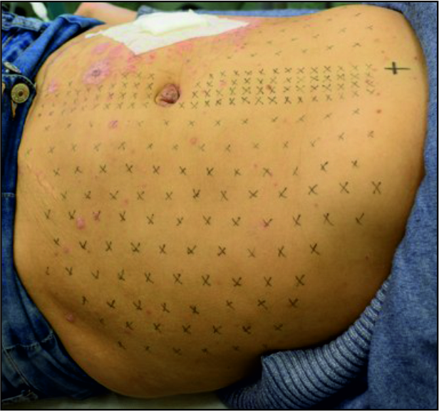
(a) Reference stage - empty abdominal cavity

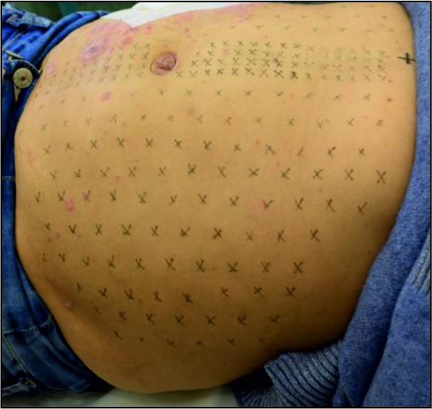
(b) Deformed stage - abdominal cavity filled with dialysis fluid

Figure 1: Stages of data acquisition. Reference and deformed stages of an abdominal wall

The 3D measurements are taken from 2D data based on photographs of the subject. The photos are taken simultaneously by four cameras installed in a specially designed stand (patent application number P.438555). The experimental set-up is shown in Figure 2, and the photo of the apparatus is in Figure 3. The stand is situated above the area of interest (abdominal wall). The distance between the cameras and the abdomen is approximately 0.5 m. The camera mounting arm is ready to rotate about the horizontal line situated perpendicularly to cranio-caudal axis of the patient. The pictures were taken in several positions of the arm changing the angle $\alpha$ every 15^∘. That enabled to collect a relevant picture set of the entire area of interest in a given state. The photos are bound to overlap, to reconstruct the 3D geometry of the abdominal wall. The Nikon D3300 cameras with 24 Mpix matrix, equipped with Nikon AF-S DX VR Nikkor 18-55mm f/3.5-5.6G II lenses have been used. Simultaneous photos are taken with the use of self-timers installed in each camera, launched in a contactless mode by an additional timer operated by a researcher. Data acquisition is presented in Figure 4(a). Calibration is provided to properly scale the collected photos. Before a proper measurement, a chequerboard calibration plate was photographed to capture the relative positions of mounted cameras. Later in the postprocessing the data, these relative positions were used to scale and reference the point cloud. Breathing influence is reduced while the pictures are shot in a full exhalation of a patient.

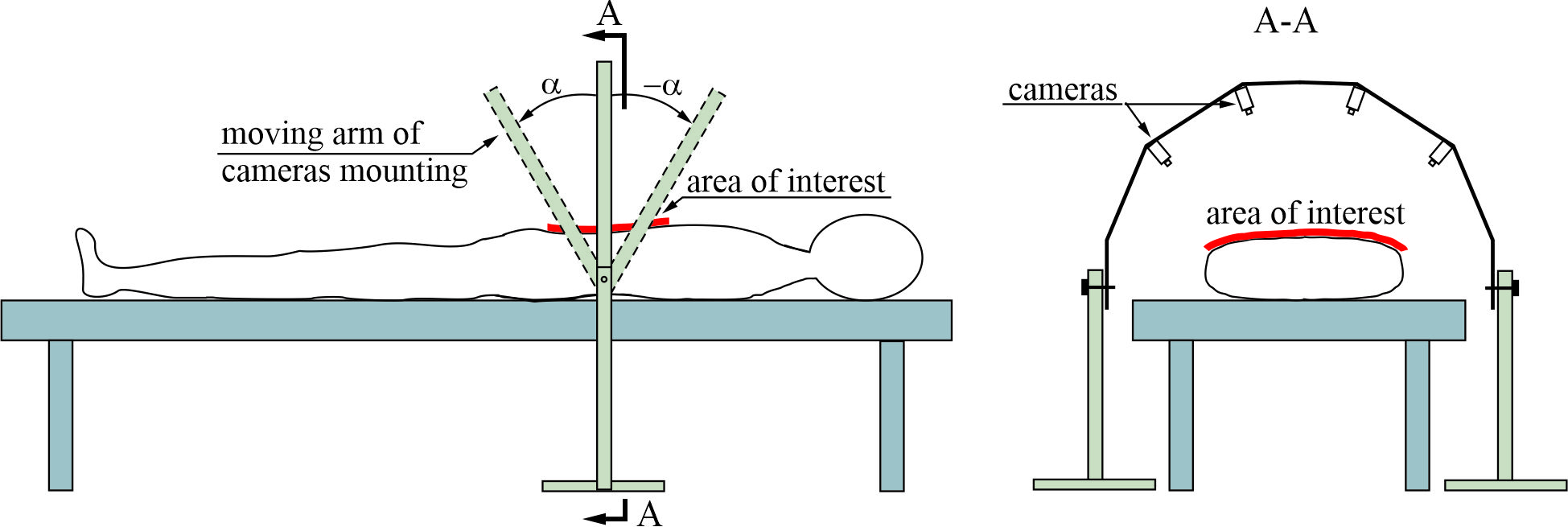
Figure 2: Experimental stand

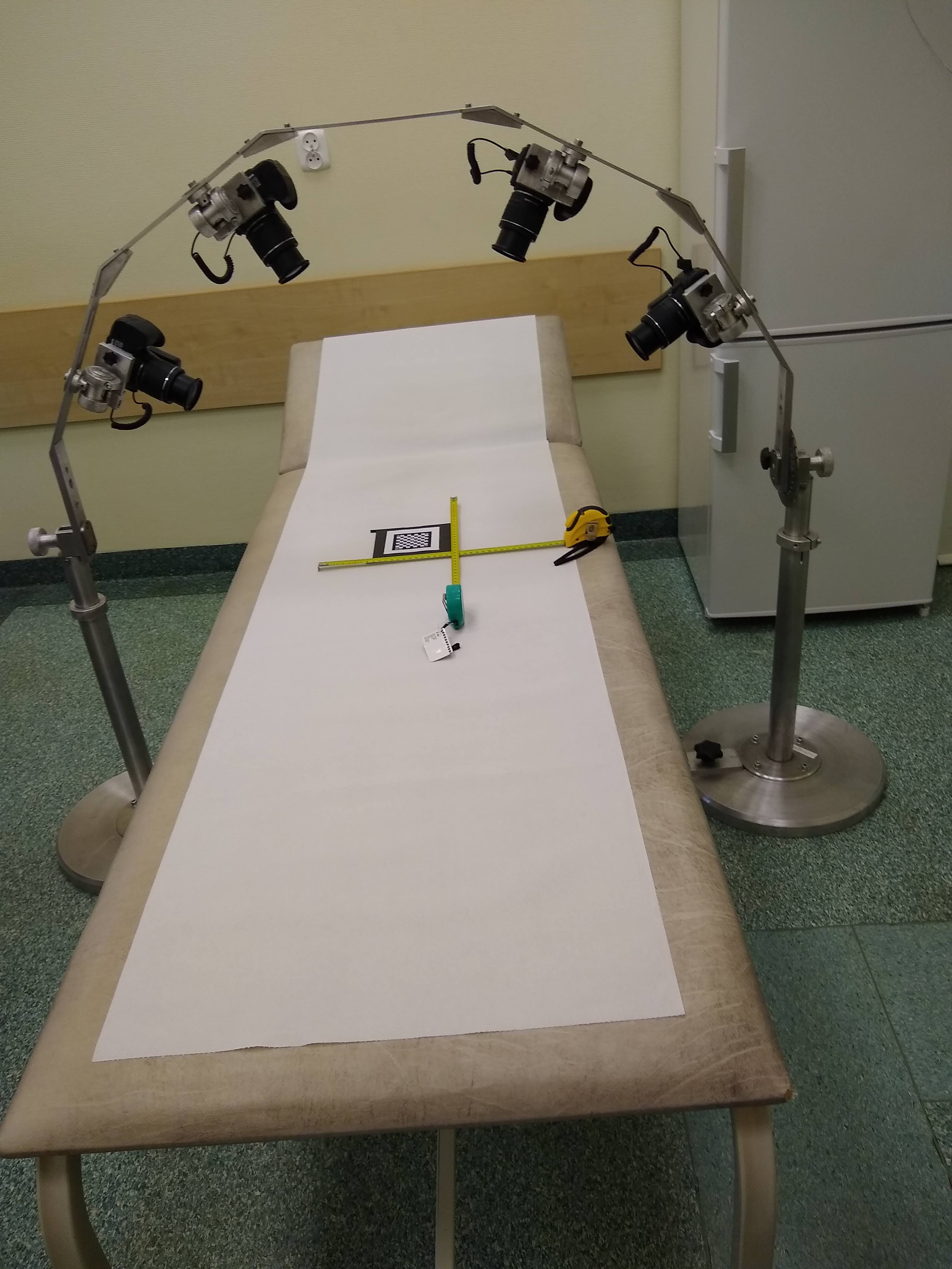
Figure 3: Experimental stand prepared for testing

The abdominal pressure is measured when the abdominal cavity is filled with a new portion of the dialysis fluid. The pressure is measured with the use of manometer connected to the dialysis bag, as regarded by Pérez Díaz et al. [2017].

2.3 Post-processing and calculation

2.3.1 Calculation of strains based on 3D geometry reconstruction

Image processing was executed with the help of Agisoft Metashape software, a commercial photogrammetry package, and RawTherapee, an open-source image-editing software.

During the camera alignment phase, relative positions of cameras are calculated and sparse point cloud of the measured object is created. Because of the subject motion (mainly respiration), photos taken from different angles in different time captured slightly different geometry. It resulted in some difficulties with automatic camera alignment. To enhance the process, we manually marked several characteristic points in each image and linked these points with neighbouring images. Camera alignment was then optimised to ensure that these points overlap in respective projection planes. Full resolution photos have been used to perform camera alignment and build the initial sparse point cloud. Coordinates of a specific camera rig position were exported. These coordinates were used later in photogrammetric models of measured subjects, so that each state (empty and full) of a subject was represented in the same coordinate system and the same scale.

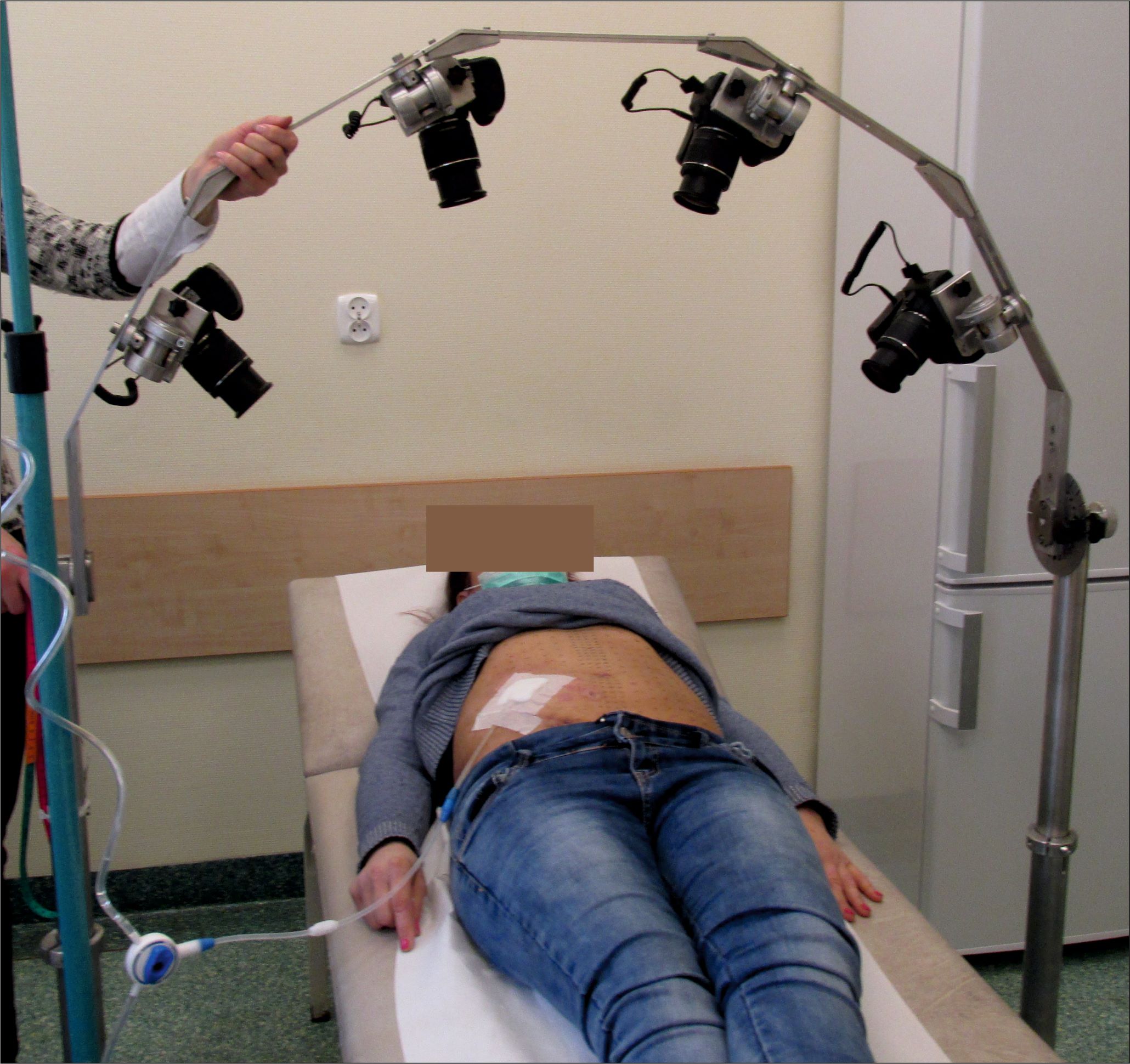
(a) Data acquisition

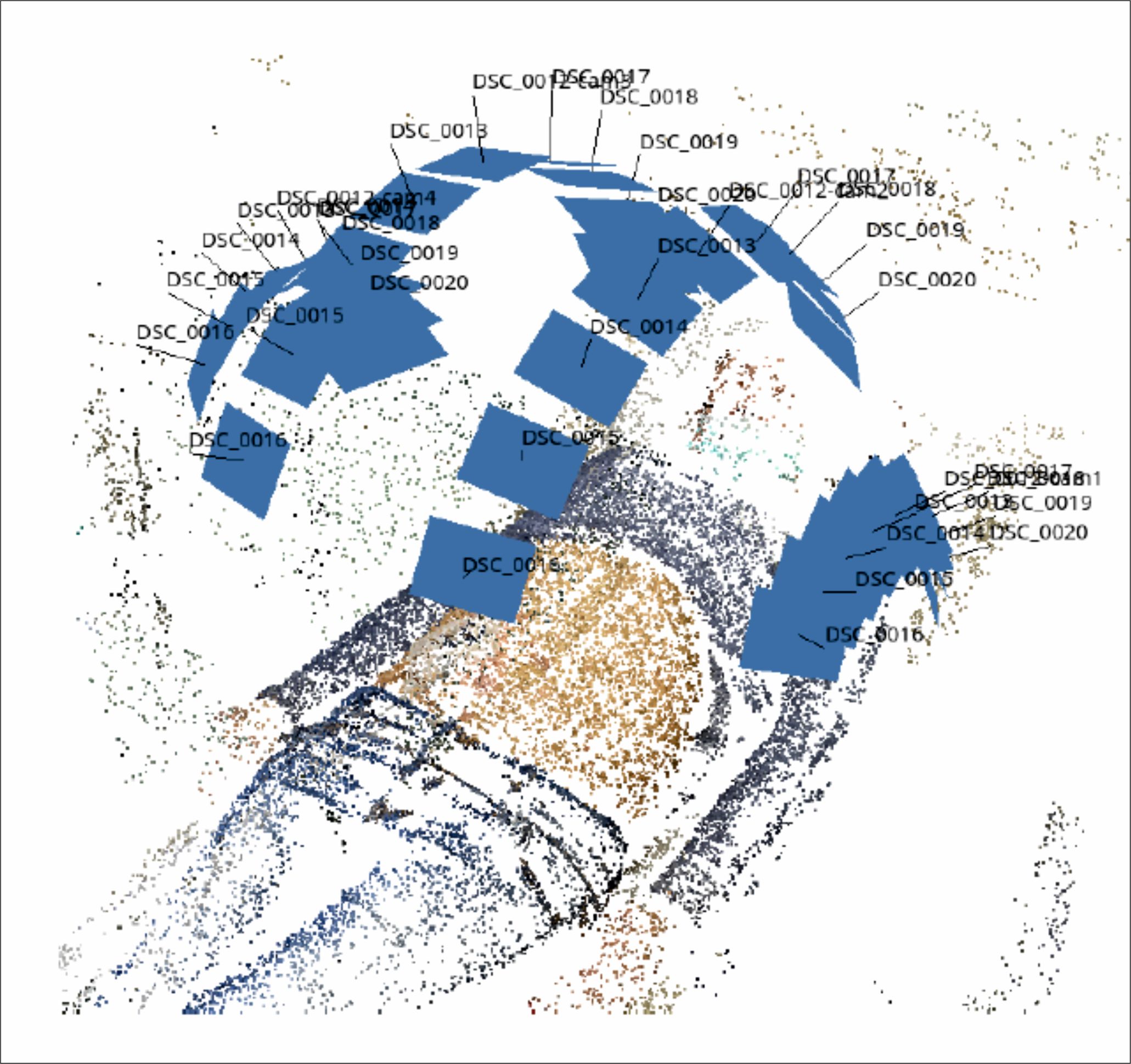
(b) Point cloud and camera positions

Figure 4: Photogrammetric measurements and corresponding first stage of data postprocessing

Based on the collected photos, the point cloud was generated, see Figure 4(b), the mapped positions of the four cameras during data acquisition are also shown. The process was conducted in both reference and deformed states. Next, the abdominal wall geometry was reconstructed in a three-dimensional space, as shown in Figure 5.

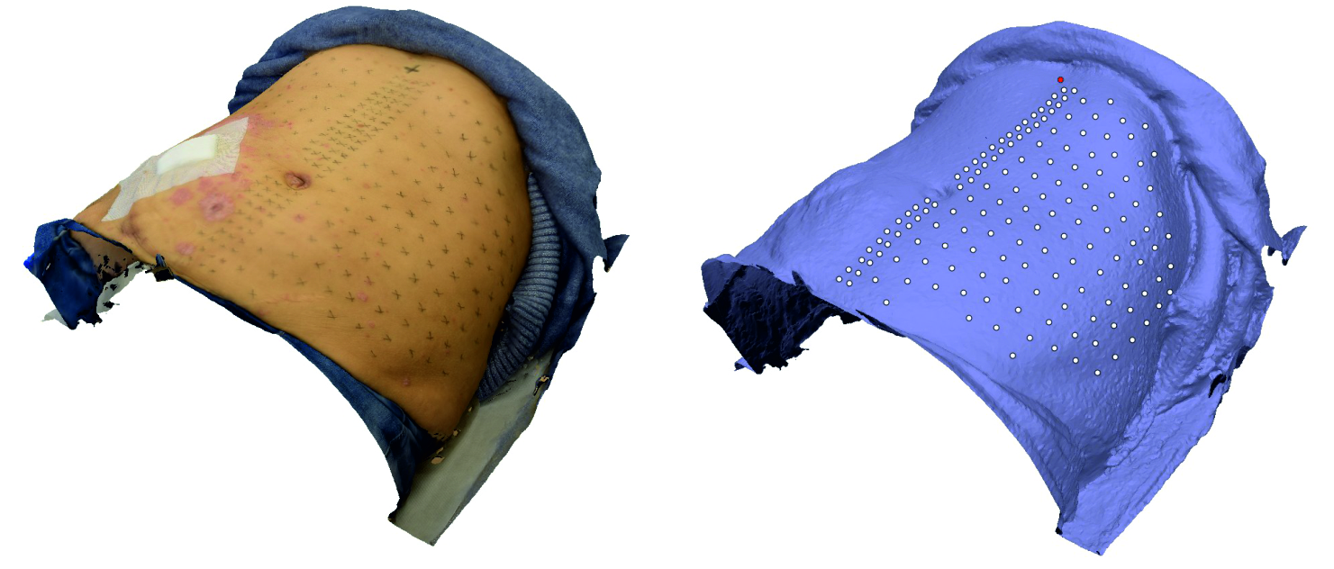
Figure 5: Photogrammetric data postprocessing - 3D reconstruction of abdominal wall geometry

The point cloud of abdominal wall was meshed using the 2D Delaunay triangulation. Twin meshes were obtained for both regarded states, as the same points were used in triangulation.

Local coordinate systems were defined in each triangle of the mesh, making two in-plane axes, x y, and a single normal axis created in accordance with the vertices. To calculate nodal displacements and strains, each triangle is considered to follow the plane strain state.

The strains are calculated using linear and nonlinear approach [Fung and Tong, 2001, Holzapfel, 2000, Wriggers, 2008]. Engineering (Cauchy) strains and Green-Lagrange strain measure are computed to compare the two approaches which are both present in the literature about the mechanics of the abdominal wall tissues and implants.

In the Lagrange description the motion of a particle in time can be described by $\mathbf{x}=\mathbf{x}(\mathbf{X},t)$, where $\mathbf{X}$ denotes its position in reference and $\mathbf{x}$ in deformed configurations. In this description, the displacement field is described by $\mathbf{U}$,

$$\mathbf{U}(\mathbf{X},t)=\mathbf{x}(\mathbf{X},t)-\mathbf{X}.$$ (1)

It can be also expressed in the Euler description as

$$\mathbf{u}(\mathbf{x},t)=\mathbf{x}-\mathbf{X}(\mathbf{x},t).$$ (2)

The deformation gradient is defined as

$$\mathbf{F}=\frac{\partial\mathbf{x}}{\partial\mathbf{X}},\quad F_{i,I}=\frac{\partial x_{i}}{\partial X_{I}}$$ (3)

and the Green-Lagrange strain tensor $\mathbf{E}$ takes the following form

$$\mathbf{E}=\frac{1}{2}\left(\mathbf{F}^{\top}\mathbf{F}-\mathbf{I}\right).$$ (4)

The strain tensor can be also expressed in terms of displacement gradient as

$$E_{ij}=\frac{1}{2}\Big{[}\frac{\partial U_{j}}{\partial X_{i}}+\frac{\partial U_{i}}{\partial X_{j}}+\frac{\partial U_{\alpha}}{\partial X_{i}}\frac{\partial U_{\alpha}}{\partial X_{j}}\Big{]}$$ (5)

that in the Euler description Euler-Almansi strain tensor takes the form of

$$e_{ij}=\frac{1}{2}\Big{[}\frac{\partial u_{j}}{\partial x_{i}}+\frac{\partial u_{i}}{\partial x_{j}}-\frac{\partial u_{\alpha}}{\partial x_{i}}\frac{\partial u_{\alpha}}{\partial x_{j}}\Big{]}.$$ (6)

The deformation gradient is computed following nonlinear finite element solution for a triangular element, where $\mathbf{X}$ and $\mathbf{x}$ are interpolated by shape functions $N_{I}$

$$\mathbf{X_{e}}=\sum_{I=1}^{n}N_{I}(\bm{\xi})\mathbf{X}_{I},\quad\mathbf{x_{e}}=\sum_{I=1}^{n}N_{I}(\bm{\xi})\mathbf{x}_{I},$$ (7)

where $\bm{\xi}$ are the coordinates of a reference element [Wriggers, 2008]. Deformation gradient of a finite element $\mathbf{F}_{e}$ can be defined as:

$$\mathbf{F}_{e}=\mathbf{j}_{e}\mathbf{J}_{e}^{-1},$$ (8)

where

$$\mathbf{j}_{e}=\frac{\partial\mathbf{x}}{\partial\bm{\xi}},\quad\mathbf{J}_{e}=\frac{\partial\mathbf{X}}{\partial\bm{\xi}},$$ (9)

The triangular element with shape functions

$$N_{1}=1-\xi-\upeta,\quad N_{2}=\xi,\quad N_{3}=\upeta,$$ (10)

leads to the Jacobi matrix (9) in the following form:

$$\mathbf{J}_{e}=\begin{bmatrix}X_{l}-X_{k}&X_{m}-X_{k}\\ Y_{l}-Y_{k}&Y_{m}-Y_{k}\end{bmatrix}$$ (11)

and

$$\mathbf{j}_{e}=\begin{bmatrix}x_{l}-x_{k}&x_{m}-x_{k}\\ y_{l}-y_{k}&y_{m}-y_{k}\end{bmatrix}.$$ (12)

When components of displacement $u_{i}$ are small, $e_{ij}$ (6) can be reduced to Cauchy infinitesimal strain tensor:

$$\varepsilon_{ij}=\displaystyle\frac{1}{2}\Big{[}\displaystyle\frac{\partial u_{j}}{\partial x_{i}}+\frac{\partial u_{i}}{\partial x_{j}}\Big{]},$$ (13)

its unabridged form reads (14)

$$\varepsilon_{xx}=\frac{\partial u}{\partial x},\quad\varepsilon_{yy}=\frac{\partial v}{\partial y},\quad\varepsilon_{xy}=\frac{1}{2}\left(\frac{\partial u}{\partial y}+\frac{\partial v}{\partial x}\right)=\varepsilon_{yx},$$ (14)

where $(x,y)$ are local nodal coordinates of every element, $(u$,$v)$ are the corresponding nodal displacements. In this case distinction between Lagrange and Euler description disappear. The strain tensor is defined in every triangle. The strains are assumed constant in element in both, reference and deformed configurations, thus nodal displacement are considered only. Two principal strains $\varepsilon_{1}$ and $\varepsilon_{2}$ satisfy the equation (15), which describes eigenvalue problem, the same for Green-Largange and Cauchy strain tensor.

$$|\varepsilon_{ij}-\varepsilon\delta_{ij}|=0$$ (15)

Each principal strain is associated with its principal axis, whose direction cosines $v^{(1)}_{j}$, $v^{(2)}_{j}$ fulfil the following:

$$(\varepsilon_{ij}-\varepsilon_{1}\delta_{ij})v^{(1)}_{j}=0,\quad(i=1,2).$$ (16)

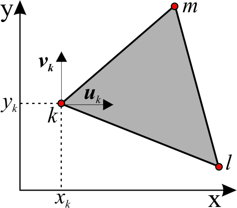
Figure 6: Triangular element in plane strain state

In a triangular element (Figure 6) undergoing plane strain, displacements of the nodes of the element are defined by two linear polynomials [Zienkiewicz, 1971].

$$u=\alpha_{1}+\alpha_{2}x+\alpha_{3}y,$$ (17)

$$v=\alpha_{4}+\alpha_{5}x+\alpha_{6}y.$$

A set of six constants $\alpha_{k}$ can be obtained by deriving two sets of three equations:

$$u_{k}=\alpha_{1}+\alpha_{2}x_{k}+\alpha_{3}y_{k},\\ u_{l}=\alpha_{1}+\alpha_{2}x_{l}+\alpha_{3}y_{l},\\ u_{m}=\alpha_{1}+\alpha_{2}x_{m}+\alpha_{3}y_{m},\\$$ (18)

with respect to $\alpha_{1}$, $\alpha_{2}$, $\alpha_{3}$, affected by on $u_{k}$, $u_{l}$, $u_{m}$, eventually finding the displacement

$$u=\frac{1}{2\Delta}[(a_{k}+b_{k}x+c_{k}y)u_{i}+(a_{l}+b_{l}x+c_{l}y)u_{j}+(a_{m}+b_{m}x+c_{m}y)u_{m}],$$ (19)

where $\Delta$ is the area of the triangle $i$, $j$, $m$ is a determinant form:

$$\Delta=\frac{1}{2}\det\begin{bmatrix}1&x_{k}&y_{k}\\ 1&x_{l}&y_{l}\\ 1&x_{m}&y_{m}\end{bmatrix}$$ (20)

and

$$a_{k}=x_{l}y_{m}-x_{m}y_{l},\quad b_{k}=y_{l}-y_{m}=y_{lm},\quad c_{k}=x_{m}-x_{l}=x_{ml}.$$ (21)

Other coefficients $a$, $b$, $c$ are derived the same way, calculating $k$, $l$, $m$.

The displacement $v$ can be obtained similar by

$$v=\frac{1}{2\Delta}[(a_{k}+b_{k}x+c_{k}y)v_{k}+(a_{l}+b_{l}x+c_{l}y)v_{l}+(a_{m}+b_{m}x+c_{m}y)v_{m}],$$ (22)

The displacement functions defined this way assure continuity on the borders with neighbouring elements, since they are linear along each triangle side. Thus the same displacements of nodes assure the same displacements between the triangles. The components $\varepsilon_{x}$, $\varepsilon_{y}$, $\gamma_{xy}$ of plane strain tensor read:

$$\begin{Bmatrix}\varepsilon_{x}\\ \varepsilon_{y}\\ 2\varepsilon_{xy}\end{Bmatrix}=\dfrac{1}{2\Delta}\begin{bmatrix}b_{k}&0&b_{l}&0&b_{m}&0\\ 0&c_{k}&0&c_{l}&0&c_{m}\\ c_{k}&b_{1}&c_{l}&b_{m}&c_{m}&b_{m}\end{bmatrix}\begin{Bmatrix}u_{k}\\ v_{k}\\ u_{l}\\ v_{l}\\ u_{m}\\ v_{m}\end{Bmatrix}.$$ (23)

The measured abdominal wall of every tested patient was reconstructed in both states, reference and deformed. The displacements of every node and strains of each triangular element were computed as described above. All calculations were performed in MATLAB environment.

2.3.2 Bayesian analysis

The presented results can be combined with the information on strain of abdominal wall available in literature to find their probabilistic distribution parameters. Following Straub and Papaioannou [2015], the classical Bayesian updating (statistical inference) can be applied to find probabilistic distribution of the model parameters based on measurements. The conditional probability of $\theta$ given the observations $\mathbf{d}$ can be calculated according to Bayes’ rule as

$$f_{\theta\mid\mathbf{d}}(\theta)=aL(\theta)f_{\theta}(\theta),$$ (24)

where $f_{\theta}$ is the prior probability density function (PDF) updated to the posterior PDF $f_{\theta\mid\mathbf{d}}$ with the use of the observations $\mathbf{d}$ represented by the likelihood function $L(\theta)$ and the normalising constant $a$ is

$$a=\frac{1}{\int_{\mathrm{R}^{n}}L(\theta)f_{\theta}(\theta)d\theta}.$$ (25)

The analysis is focused on maximum $\varepsilon_{1}$ observed in abdominal wall of a patient because maximum strains can be interesting from the viewpoint of choice of surgical mesh with an appropriate strain range. Let us assume that $\mathcal{X}$, standing for the maximum $\varepsilon_{1}$, is a Gaussian variable with unknown mean $\theta$ and fixed standard deviation. The likelihood function $L(\theta)$ is a Gaussian variable with mean $\theta$ and fixed standard deviation $\sigma_{\mathcal{X}}=3.3\%$ with a conjugate prior — Gaussian variable whose parameters are $\mu_{\theta}=13.25\%$ and $\sigma_{\theta}=5.27\%$. The parameters of prior distributions are assumed that 90th percentile is 20%, (in top range of values reported in the literature for similar value of intraabdominal pressure, Le Ruyet et al. [2020]) and 1st percentile is 1%. In this conjugate prior case the analytical solution is known and the posterior $\theta$ is Gaussian with the mean following the formula:

$$\mu_{\theta\mid\mathbf{d}}=\frac{\mu_{\theta}/\sigma_{\theta}^{2}+m\bar{d}/\sigma_{\mathcal{X}}^{2}}{1/\sigma_{\theta}^{2}+m/\sigma_{\mathcal{X}}^{2}},$$ (26)

and the standard deviation

$$\sigma_{\theta\mid\mathbf{d}}=\left(\frac{1}{1/\sigma_{\theta}^{2}+m/\sigma_{\mathcal{X}}^{2}}\right)^{1/2},$$ (27)

where $m=7$ is the number of observations $\mathbf{d}$ (Table 2) of the random variable $\mathcal{X}$ and $\bar{d}$ is the mean of $\mathbf{d}$. Since $\theta$ is a Gaussian variable, the predictive distribution of $\mathcal{X}$ with unknown mean may be found, it is also a Gaussian variable with the same mean, $\mu=\mu_{\theta\mid\mathbf{d}}$ and standard deviation, $\sigma=\sqrt{\sigma_{\theta\mid\mathbf{d}}^{2}+\sigma_{\mathcal{X}}^{2}}$.

3 Results and discussion

The intraabdominal pressure measured after full introduction of dialysis fluid is presented in Table 2. The table also includes the minimum, maximum and median values of principal strains, both Cauchy (engineering) and Green-Lagrange, observed in all cases. Maximum absolute difference between Green-Lagrange and engineering strains equals 1.45% (7.9% relative difference with respect to Green-Lagrange value). This value was observed in case of P1. Mean absolute difference, in terms of patients, between Green-Lagrange and engineering strains equals 0.89% (6.2% relative difference with respect to Green-Lagrange value) in case of maximum value of $\varepsilon_{1}$, 0.23% (3.7% relative difference with respect to Green-Lagrange value) in case of minimum value of $\varepsilon_{2}$ and 0.19% (3.1% relative difference with respect to Green-Lagrange value) and 0.04% (1.9% relative difference with respect to Green-Lagrange value) for median of $\varepsilon_{1}$ and $\varepsilon_{2}$, respectively. The differences between engineering and Green-Lagrange strains statistics can be observed on the boxplots (Figure 7). The further discussion is based on the values of Cauchy strains, since the analysis of both, Cauchy and Green-Lagrange strain values are relatively similar and lead to similar conclusions.

Figures 8–14 show maps of maximum $\varepsilon_{1}$ and minimum $\varepsilon_{2}$, the principal strains obtained for tested subjects. The colours in maps are related to the value of principal strains. The principal strain direction are line-marked in every triangular element. The maps show diverse spatial distribution of principal strains in the abdominal wall of the patients. The non-uniform character of principal strains is also observable in histograms (Figure 15) and boxplots (Figure 7).

Taking into the account the prior belief, the posterior mean of maximum $\varepsilon_{1}$ is a Gaussian variable with mean 12.71% and standard deviation 1.21%. That leads to predictive distribution of maximum $\varepsilon_{1}$ with the same mean and standard deviation 3.52%. Its coefficient of variation equals 28% belonging to the variability range observed in biological materials [Cook et al., 2014]. Such variability should be further included in the modelling. The obtained probabilistic form could be next propagated in surgical mesh models to consider uncertainty of maximum strains in the analysis of implants [Szepietowska et al., 2018].

Table 2: Intraabdominal pressure and corresponding strain observed in case of each patient

No.	pressure	Principal strains* [%]
	[cmH2O]	Maximum			Minimum			Median
		$\varepsilon_{1}$	$E_{1}$		$\varepsilon_{2}$	$E_{2}$		$\varepsilon_{1}$	$E_{1}$	$\varepsilon_{2}$	$E_{2}$
P1	15	17.0	18.5		-4.6	-4.4		7.1	7.3	3.5	3.6
P2	11.5	12.4	13.2		-10.0	-9.4		4.1	4.3	-2.2	-2.2
P3	11.5	13.3	14.3		-0.8	-0.7		6.5	6.7	2.4	2.5
P4	11	13.2	14.1		-2.6	-2.5		6.6	6.9	2.2	2.2
P5	18.5	7.3	7.6		-2.5	-2.4		4.1	4.2	0.3	0.3
P6	11.5	10.0	10.5		-10.1	-9.5		4.3	4.4	0.7	0.7
P7	15.5	15.6	16.9		-6.9	-6.6		7.7	8.0	3.4	3.4

* $\varepsilon$ denotes Cauchy strain, $E$ denotes Green-Lagrange strain

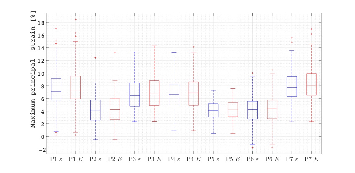
(a) Maximum principal strain

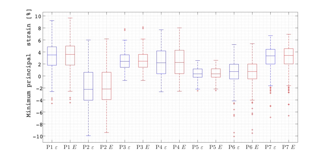
(b) Minimum principal strain

Figure 7: Boxplots of principal Cauchy ($\varepsilon$, blue boxes) and Green-Lagrange ($E$, red boxes) strains. The central line is the median, edges of box are the 25th and 75th percentiles (distance between top and bottom edge is interquartile range), whiskers extend to furthest data points but outliers are marked by red ’+’ (beyond 1.5 times interquartile range away from top or bottom of the box)

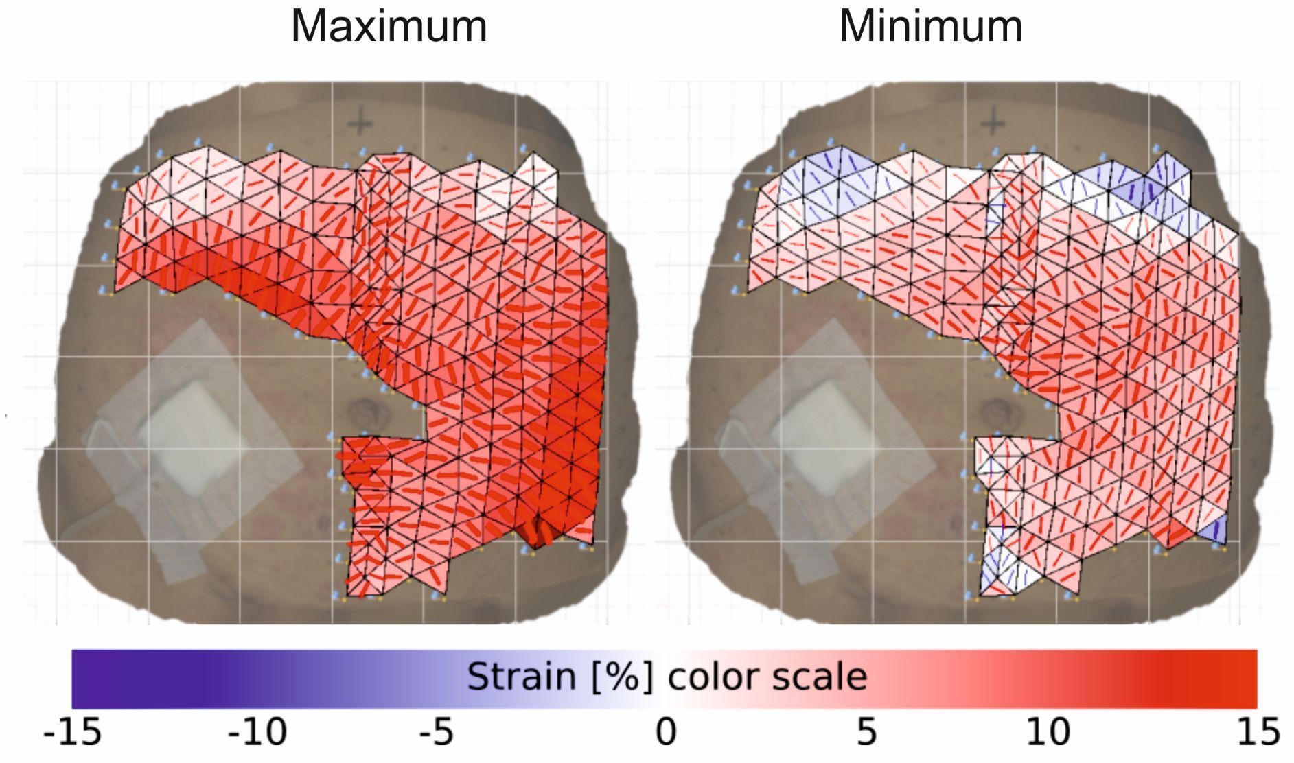
Figure 8: Principal maximum and minimum Cauchy strains with principal directions for Patient P1

Figure 9: Principal maximum and minimum Cauchy strains with principal directions for Patient P2

Figure 10: Principal maximum and minimum Cauchy strains with principal directions for Patient P3

Figure 11: Principal maximum and minimum Cauchy strains with principal directions for Patient P4

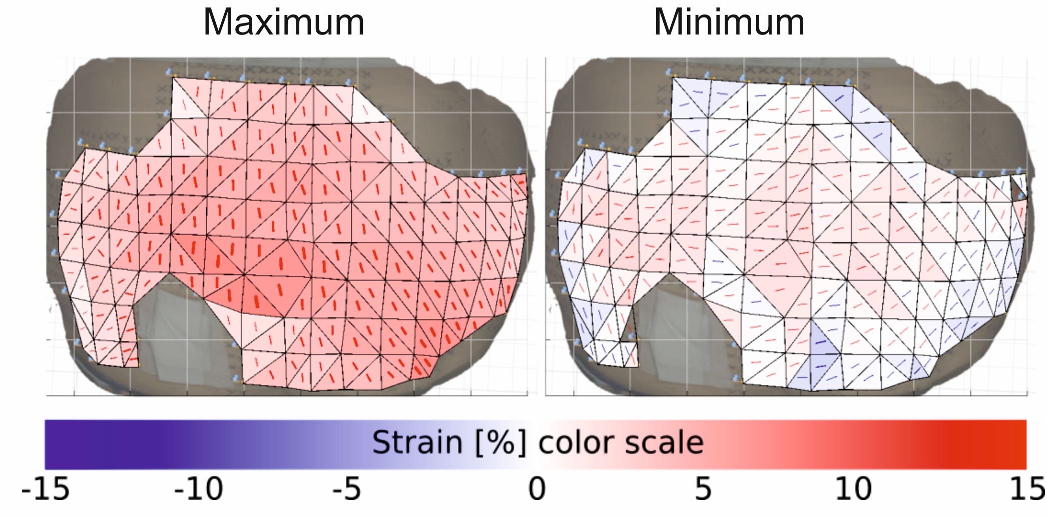
Figure 12: Principal maximum and minimum Cauchy strains with principal directions for Patient P5

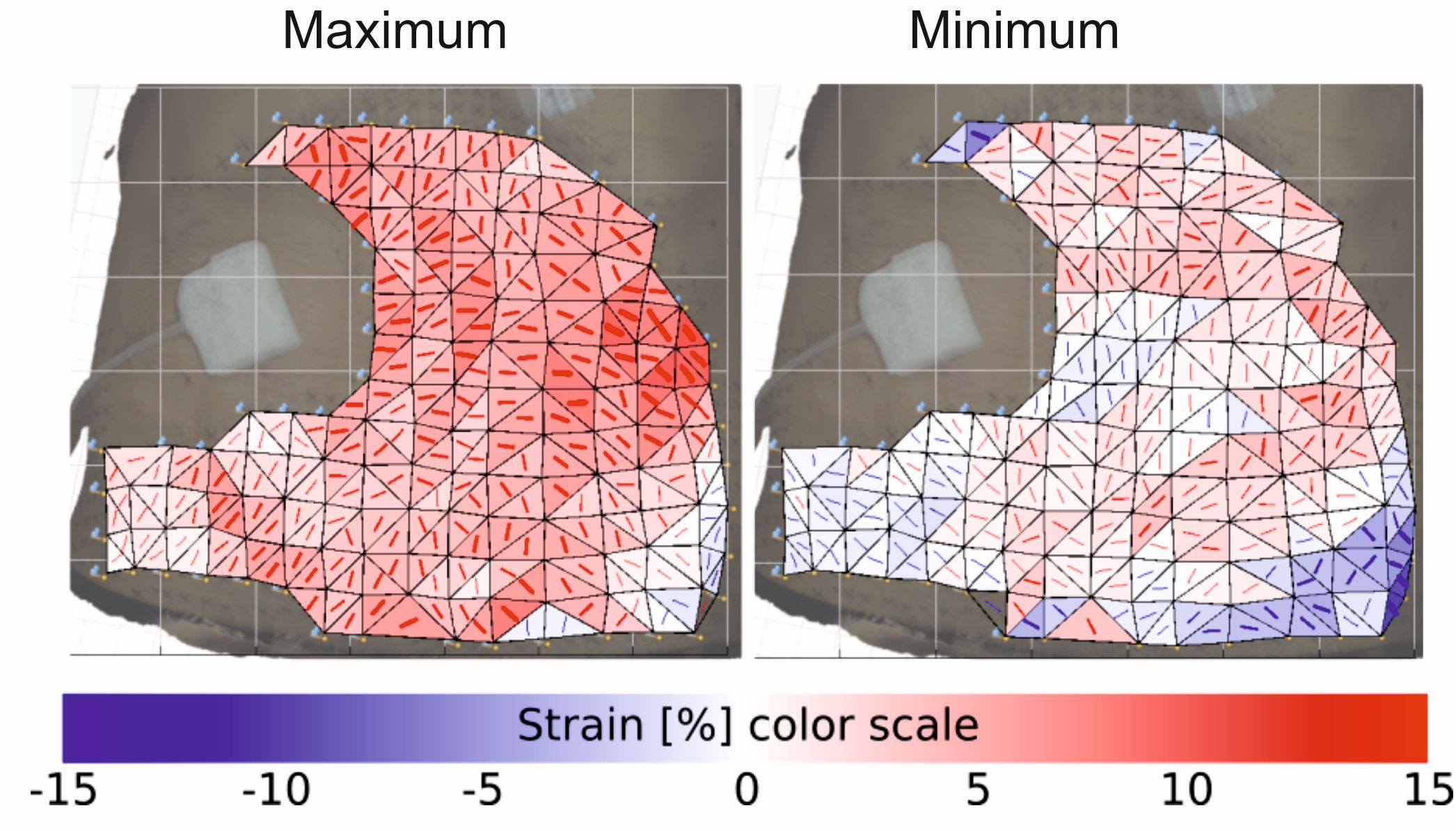
Figure 13: Principal maximum and minimum Cauchy strains with principal directions for Patient P6

Figure 14: Principal maximum and minimum Cauchy strains with principal directions for Patient P7

The lowest maximum $\varepsilon_{1}$ was observed in the Patient P5 case, with the highest intraabdominal pressure referring to the same amount of fluid as in other patients (see Table 2). This implies a high stiffness of the abdominal wall. The ranges of strains, $\varepsilon_{1}$ and $\varepsilon_{2}$, are the narrowest amongst all patients of this case (see Figure 7).

The variability can be seen among all tested patients (see Figures 15 and 7). However, similarities between selected patients may be observed. The median values are similar between patients of similar age and intraabdominal pressure value, i. e. between Patients P3 and P4 (65 years old, 11.5 cmH₂0 and 64 years old, 11.5 cmH₂0, respectively), between Patients P5 and P6 (both are 34 years old, but different intraabdominal pressure: 18.5 and 11.5 cmH₂0, respectively) and finally between Patients P1 and P7 (46 years old, 15 cmH₂0 and 47 years old, 15.5 cmH₂0, respectively). A sole Patient P2 shows a negative median of $\varepsilon_{2}$. In this case negative values of the $\varepsilon_{2}$ appear in large part of abdominal surface (Figure 9).

In this study, it can be seen that the values of strains of the outer surface of the abdominal wall are mostly positive. However, negative strains are also observed (see Figures 8-13, 15). The presence of negative strains may be linked with heterogeneity of the abdominal wall related to its complex architecture. Secondly, it can be influenced by prestrain observed in living tissues as well as boundary conditions, related to the attachment of tissues to the rib cage and pelvis, as the negative values appear mainly in the vicinity of the chest and hips. In addition, it can also be influenced by the coupling of membrane forces and bending.

The abdominal wall health conditions of patients undergoing measurements is diverse. Patients P2-P5 have or are suspected to have abdominal hernia. Although, the presence of hernia is expected to affect the results, any hernia effect is observed in this study. The strain range of Patient P5 is in range 7.3%–0.5%, -2.5–2.6%, in case of $\varepsilon_{1}$ and $\varepsilon_{2}$, and first principal directions is close to cranio-caudal axis without a visible hernia effect. More patients should be investigated in the light of hernia impact on the registered strains of abdominal wall.

The obtained principal strain directions do not follow the same pattern in all patients, instead they vary along the abdominal wall of individual patient. The Patients P2, P3 and P5 show it more regular. The first principal strain direction around a mid-line is most clearly aligned along the cranio-caudal direction in the case of Patient P5 only. This orientation is consistent with the results of studies on the abdominal walls of human cadavers subjected to intraabdominal pressure described by Le Ruyet et al. [2020]. The disturbance in principal directions observed in other cases analysed here may be caused by active work of muscles associated with breathing. The presented deformation is mainly related to passive behaviour of myofascial system of abdominal wall under dialysis fluid introduction. However, some active muscle contribution of a breathing patient may possibly affect the strain results.

The change of principal directions is observable in areas close to the peritoneal catheter dressing in some patients, e.g. P1, P4, P6. The patch creates a local disturbance in the strain field of the external surface of the abdominal wall. Thus, with extreme caution, the directions of principal strains in the area of the patch should be interpreted. Therefore, in future identification of mechanical properties of abdominal wall based on this study, the part of abdominal wall close to catheter should be neglected, while affected by the patch. This is a limitation in capturing the asymmetry of the abdominal wall. This asymmetry is indicated in several studies, e.g., Jourdan et al. [2020] reported geometric asymmetry of abdominal muscles. Todros et al. [2019] observed mostly symmetrical displacement of rectus muscle and a more pronounced asymmetry in the case of lateral muscles during muscle contraction. Nevertheless, in the existing research on numerical models of the abdominal wall, the material parameters are usually symmetric [He et al., 2020], even a full symmetric model is assumed with respect to the sagittal plane [Pachera et al., 2016].

In addition to patient variability in factors such as age, BMI, and health condition, the patients differ in the measured area. This is bounded by a patch covering the catheter placed in different regions of the abdominal wall.

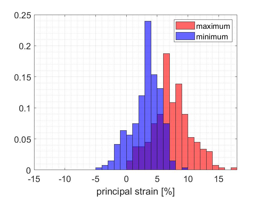
(a) Patient P1

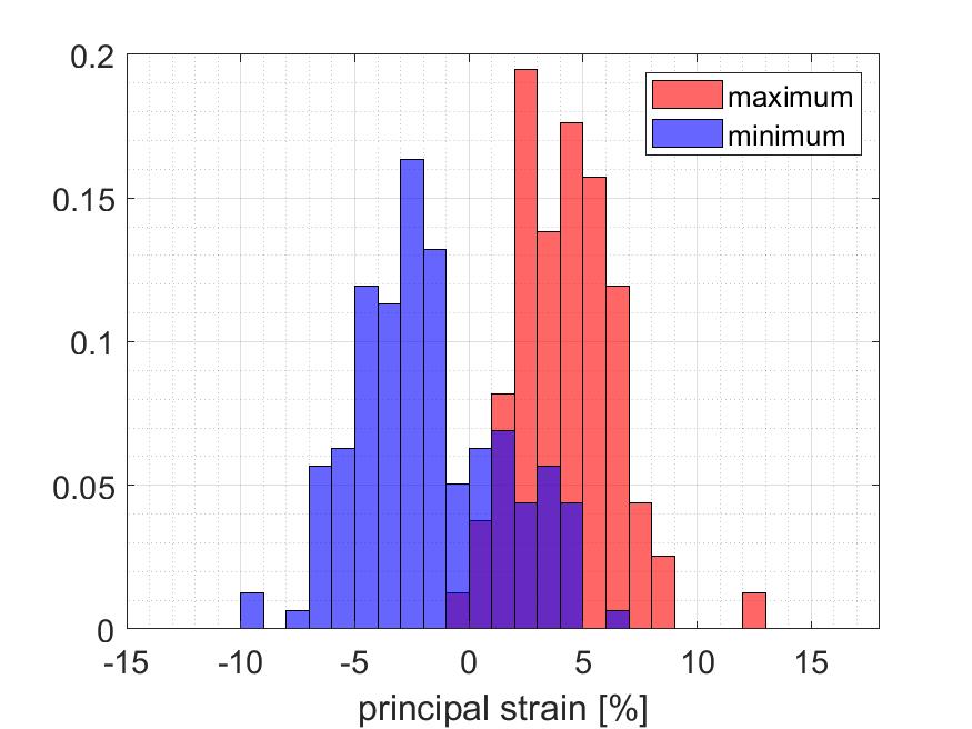
(b) Patient P2

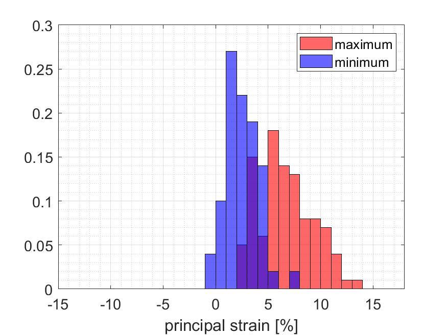
(c) Patient P3

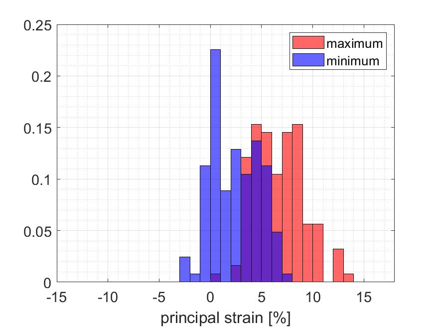
(d) Patient P4

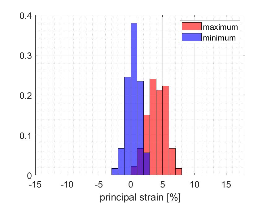
(e) Patient P5

(f) Patient P6

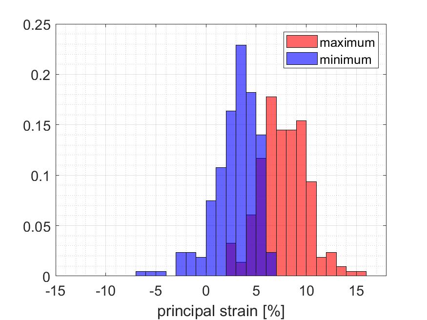
(g) Patient P7

Figure 15: Normalized histograms of principal Cauchy strains; maximum $\varepsilon_{1}$ (red) and minimum $\varepsilon_{2}$ (blue)

Figures 16–19 show the abdominal wall nodal displacements of two oldest and two youngest patients, respectively, which includes also patients with the highest BMI (Figure 16) and the lowest BMI (Figure 19). The maximum displacement in cases of the oldest patients, P3 and P4 (similar age but quite different BMI), is similar and equal to 19.3 mm and 19.9 mm respectively (see Figures 16 and 17). In the case of the youngest patients, P5 and P6, both at age of 34, and again different BMI, the registered maximum displacement of the abdomen is higher (21.5 mm and 22.4 mm) but again these values are quite similar to each other (see Figures 18 and 19). The plot of displacements for P6 differs from other patients. This patient has the lowest BMI (20) that determines the shape of the abdominal wall and probably also its mechanical behaviour.

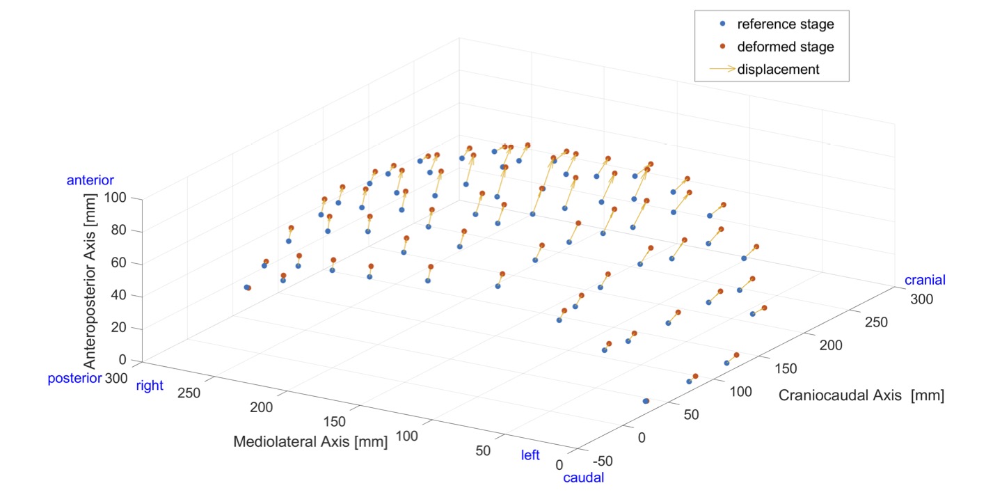
Figure 16: Patient P3 displacements (range from 0.6 to 19.3 mm)

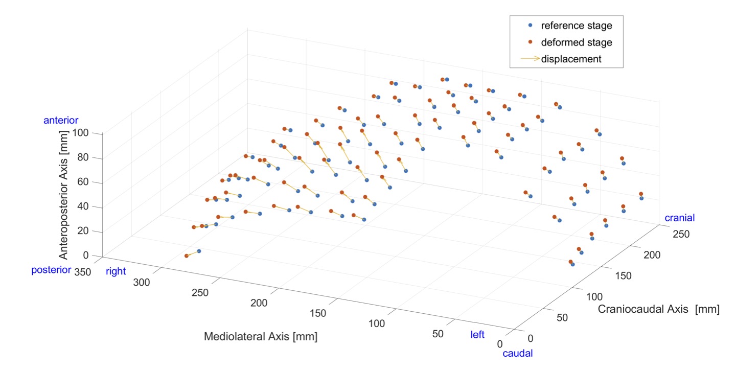
Figure 17: Patient P4 displacements (range from 3.3 to 19.9 mm)

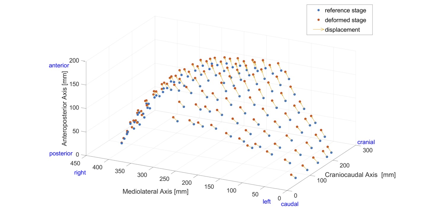
Figure 18: Patient P5 displacements (range from 4.0 to 21.5 mm)

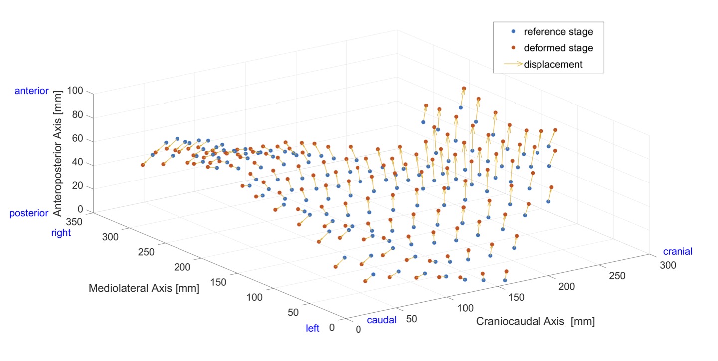
Figure 19: Patient P6 displacements (range from 6.2 to 22.4 mm)

Although other studies presented principal strains of abdominal wall under diverse conditions (in or ex vivo, loading condition etc.), the present results are partially referred to the values reported in literature.

• our past study [Szymczak et al., 2012] adressed strains on the living abdominal wall under activities like bending or stretching were analysed. That study also shows a high inter patients variability. The observed range of strains is higher there, in a given oblique direction the mean values of strains reaches even 34%. However, the investigated group was younger (23–25 years old) and healthy. Nevertheless, a high difference in strain ranges in this study and in the present research, was mainly caused by different loading conditions, inducing active muscle behaviour, while the present study refers to their mostly passive behaviour under slow change of intraabdominal pressure. Furthermore, torso bending is considered decisive to trigger high deformations of he abdominal wall. This was shown in the in vivo study by Lubowiecka et al. [2020], here the elongation of surgical meshes implanted to the abdomen was tested while under torso bending. A numerical study by Szymczak et al. [2017] suggests that deformation of abdominal wall caused by such activities may provoke higher forces in the joints connecting surgical mesh to the abdominal wall than the loading produced by intraabdominal pressure.

• Le Ruyet et al. [2020] presented strains in myofascial abdominal walls (without fat and subcutaneous fat) of human cadavers subjected to cycles of pressure, reporting high variability amongst studied samples. The research was aimed at comparing suturing techniques, the results for intact linea alba were also shown. The maximum strains and their directions of this inquiry are similar to the present study when refer to a similar range of pressure applied to the abdominal wall. A single sample reveals larger strain value in the sample domain (Green-Lagrange strains close to 20% in the point in the midline).

• In the in vivo research on protruded and contracted human abdominal walls described by Breier et al. [2017], the maximum observed strain reached 60%. Similarly to our study, the authors observed high variability among the patients.

• Podwojewski et al. [2013] obtained, in their in vitro study, an average value of 13.7% of the first principal Lagrange strain on the outer surface of the abdominal wall of a porcine abdominal wall subjected to pressure. The pressure was equal to 50 mmHg (around 68 cmH₂0), higher compared to the present research.

It can be stated that the range of principal strains of the ongoing research is consistent with the results reported in the literature related to strain in the abdominal wall subjected to similar loading.

It should be noted that the abdominal wall is a complex multi-layered structure of components with different fibers alignments. It contains the: skin, subcutaneous tissue, superficial fascia, rectus abdominis muscle, external oblique muscle, internal oblique muscle, transversus abdominis muscle, transversalis fascia, preperitoneal adipose and areolar tissue, and peritoneum. Nerves, blood vessels, and lymphatics are present throughout. The contour and thickness of the abdomen is dependent upon age, muscle mass, muscle tone, obesity, intra-abdominal pathology, parity, and posture. Integrity of the anterior abdominal wall is primarily dependent upon the abdominal muscles and their conjoined tendons. The average thickness of rectus abdominis muscle and abdominal subcutaneous fat tissue measured by Kim et al. [2012] with the use of computer tomography, was 10 mm, and the average subcutaneous tissue thickness equalled 24 mm. Nevertheless, in our study only the strains of the outer surface of the abdominal wall are investigated. Therefore the connective tissues and muscles considered important are not directly observed. The latter issue is a possible limitation of the study. However Tran et al. [2014] showed that the contribution of skin and adipose tissue in the strains of the abdominal wall under pressure is not as decisive as, say, rectus sheath.

Next limitation is that nonlinear behaviour of the abdominal wall in response to intra-abdominal pressure is not captured in this study. Our aim was to interfere with the medical procedure as little as possible. Therefore, since standard methodology of peritoneal dialysis does not assume measurements of IAP in intermediate states, the pressure measurements have been performed after filling peritoneal cavity with 2000 ml of dialysis fluid.The measurements need to be limited for the sake of patient’s safety because additional measurements of intra-abdominal pressure would have been associated with an increased risk of peritoneal infection.

This study is focused on strains. However, the results can be further used in the identification of the mechanical properties of abdominal wall. That will require deep consideration of various aspects of this issue, such as nonlinearity, anisotropy, etc. In addition, residual stresses can affect the mechanical response of the entire system, which should be considered in future simulations and the identification of abdominal stiffness [Rausch and Kuhl, 2013]. The reference configuration of drained abdominal wall analysed in the current study may not be stress free.

It should be noted that intraabdominal pressure is considered a load in much of the research on numerical abdominal wall modelling [Pachera et al., 2016, Hernández-Gascón et al., 2013]. The presented results can be incorporated to validate numerical models of the anterior abdominal wall.

4 Conclusions

The methodology proposed in the study brings the deformation of the living human abdominal wall corresponding to the intraabdominal pressure measured during peritoneal dialysis. This approach is successfully applied for a group of patients with various abdominal wall health status. The dedicated experimental stand simplifies geometry measurement of a living object. Although, the post-processing of the photogrammetric data is more time consuming when compared to commercial digital image correlation systems, the measurement alone can be performed relatively quickly. This fact, combined with the ease and quick assembly, the absence of wires and the relatively small room required, makes the mobile experimental stand suitable for use in hospitals during standard PD fluid exchange.

The study presents the values and spatial distribution of strains observed on external surface of abdominal wall of each patient. Cauchy and Green-Lagrange strains are shown. The maximum principal Cauchy strains vary from 7.3 to 17%, the median of first principal directions varies from 4.1 to 7.7% throughout the patients. The set of maximum values shows a mean 12.7%. The observed intraabdominal pressure ranges from 11 to 18.5 cmH₂O. The obtained principal strains and their directions indicate variability in a patient domain.

High variability observed between the subjects in each study indicates high mechanical parameter variability of the abdominal wall. This justifies a need for patient-specific approach towards treatment optimisation of ventral hernias. However, in the future, a larger group of patients should be tested to investigate the effect of various parameters, e.g. the age, BMI or health condition, to possibly affect the range of strains of human living abdominal wall.

The presented work is the next step towards the recognition of mechanics of living human abdominal wall. The presented approach can be further expanded to identify the mechanical properties of human abdominal wall based on in vivo measurements, performed in non-invasive and relatively inexpensive way. The results can also be applied to validate other computational models of the abdominal wall. The research entirety is aimed at improving abdominal hernia repair as reliable computational models will enable in silico analysis and optimisation of abdominal hernia treatment parameters.

References

- Al-Hwiesh et al. [2011] Al-Hwiesh, A., Al-Mueilo, S., Saeed, I., Al-Muhanna, F.A., 2011. Intraperitoneal pressure and intra-abdominal pressure: Are they the same? Peritoneal Dialysis International 31, 315–319. PMID: 21357935.
- Anurov et al. [2012] Anurov, M., Titkova, S., Oettinger, A., 2012. Biomechanical compatibility of surgical mesh and fascia being reinforced: dependence of experimental hernia defect repair results on anisotropic surgical mesh positioning. Hernia 16, 199–210.
- Armesto et al. [2009] Armesto, J., Lubowiecka, I., Ordóñez, C., Rial, F.I., 2009. Fem modeling of structures based on close range digital photogrammetry. Automation in Construction 18, 559–569.
- Astruc et al. [2018] Astruc, L., De Meulaere, M., Witz, J.F., Nováček, V., Turquier, F., Hoc, T., Brieu, M., 2018. Characterization of the anisotropic mechanical behavior of human abdominal wall connective tissues. Journal of the Mechanical Behavior of Biomedical Materials 82, 45–50.
- Avril et al. [2008] Avril, S., Bonnet, M., Bretelle, A.S., Grédiac, M., Hild, F., Ienny, P., Latourte, F., Lemosse, D., Pagano, S., Pagnacco, E., et al., 2008. Overview of identification methods of mechanical parameters based on full-field measurements. Experimental Mechanics 48, 381–402.
- Barone et al. [2015] Barone, W.R., Amini, R., Maiti, S., Moalli, P.A., Abramowitch, S.D., 2015. The impact of boundary conditions on surface curvature of polypropylene mesh in response to uniaxial loading. Journal of Biomechanics 48, 1566–1574.
- Breier et al. [2017] Breier, A., Bittrich, L., Hahn, J., Spickenheuer, A., 2017. Evaluation of optical data gained by aramis-measurement of abdominal wall movements for an anisotropic pattern design of stress-adapted hernia meshes produced by embroidery technology, in: IOP Conference Series: Materials Science and Engineering, IOP Publishing. p. 062002.
- Calvo et al. [2014] Calvo, B., Sierra, M., Grasa, J., Munoz, M., Pena, E., 2014. Determination of passive viscoelastic response of the abdominal muscle and related constitutive modeling: Stress-relaxation behavior. Journal of the Mechanical Behavior of Biomedical Materials 36, 47–58.
- Cook et al. [2014] Cook, D., Julias, M., Nauman, E., 2014. Biological variability in biomechanical engineering research: Significance and meta-analysis of current modeling practices. Journal of Biomechanics 47, 1241–1250.
- Cooney et al. [2016] Cooney, G.M., Lake, S.P., Thompson, D.M., Castile, R.M., Winter, D.C., Simms, C.K., 2016. Uniaxial and biaxial tensile stress–stretch response of human linea alba. Journal of the Mechanical Behavior of Biomedical Materials 63, 134–140.
- Deeken and Lake [2017] Deeken, C.R., Lake, S.P., 2017. Mechanical properties of the abdominal wall and biomaterials utilized for hernia repair. Journal of the Mechanical Behavior of Biomedical Materials 74, 411–427.
- Durand et al. [1996] Durand, P.Y., Chanliau, J., Gambéroni, J., Hestin, D., Kessler, M., 1996. Measurement of hydrostatic intraperitoneal pressure: a necessary routine test in peritoneal dialysis. Peritoneal Dialysis International 16, 84–87.
- Fung and Tong [2001] Fung, Y.C., Tong, P., 2001. Classical and Computational Solid Mechanics (Advanced Series in Engineering Science). World Scientific Publishing Company.
- Grasa et al. [2016] Grasa, J., Sierra, M., Lauzeral, N., Munoz, M., Miana-Mena, F., Calvo, B., 2016. Active behavior of abdominal wall muscles: Experimental results and numerical model formulation. Journal of the Mechanical Behavior of Biomedical Materials 61, 444–454.
- He et al. [2020] He, W., Liu, X., Wu, S., Liao, J., Cao, G., Fan, Y., Li, X., 2020. A numerical method for guiding the design of surgical meshes with suitable mechanical properties for specific abdominal hernias. Computers in Biology and Medicine 116, 103531.
- Hernández et al. [2011] Hernández, B., Pena, E., Pascual, G., Rodriguez, M., Calvo, B., Doblaré, M., Bellón, J., 2011. Mechanical and histological characterization of the abdominal muscle. a previous step to modelling hernia surgery. Journal of the Mechanical Behavior of Biomedical Materials 4, 392–404.
- Hernández-Gascón et al. [2013] Hernández-Gascón, B., Mena, A., Pena, E., Pascual, G., Bellón, J., Calvo, B., 2013. Understanding the passive mechanical behavior of the human abdominal wall. Annals of Biomedical Engineering 41, 433–444.
- Holzapfel [2000] Holzapfel, G.A., 2000. Nonlinear solid mechanics : a continuum approach for engineering. Wiley.
- Jourdan et al. [2021] Jourdan, A., Le Troter, A., Daude, P., Rapacchi, S., Masson, C., Bège, T., Bendahan, D., 2021. Semiautomatic quantification of abdominal wall muscles deformations based on dynamic mri image registration. NMR in Biomedicine 34, e4470.
- Jourdan et al. [2020] Jourdan, A., Soucasse, A., Scemama, U., Gillion, J.F., Chaumoitre, K., Masson, C., Bege, T., For "Club Hernie", 2020. Abdominal wall morphometric variability based on computed tomography: Influence of age, gender, and body mass index. Clinical Anatomy 33, 1110–1119.
- Junge et al. [2001] Junge, K., Klinge, U., Prescher, A., Giboni, P., Niewiera, M., Schumpelick, V., 2001. Elasticity of the anterior abdominal wall and impact for reparation of incisional hernias using mesh implants. Hernia 5, 113–118.
- Kahan et al. [2018] Kahan, L.G., Lake, S.P., McAllister, J.M., Tan, W.H., Yu, J., Thompson, D., Brunt, L.M., Blatnik, J.A., 2018. Combined in vivo and ex vivo analysis of mesh mechanics in a porcine hernia model. Surgical Endoscopy 32, 820–830.
- Kim et al. [2012] Kim, J., Lim, H., Lee, S.I., Kim, Y.J., 2012. Thickness of rectus abdominis muscle and abdominal subcutaneous fat tissue in adult women: correlation with age, pregnancy, laparotomy, and body mass index. Archives of Plastic Surgery 39, 528.
- Kirilova et al. [2011] Kirilova, M., Stoytchev, S., Pashkouleva, D., Kavardzhikov, V., 2011. Experimental study of the mechanical properties of human abdominal fascia. Medical Engineering & Physics 33, 1–6.
- Le Ruyet et al. [2020] Le Ruyet, A., Yurtkap, Y., den Hartog, F., Vegleur, A., Turquier, F., Lange, J., Kleinrensink, G., 2020. Differences in biomechanics of abdominal wall closure with and without mesh reinforcement: A study in post mortem human specimens. Journal of the Mechanical Behavior of Biomedical Materials 105, 103683.
- Levillain et al. [2016] Levillain, A., Orhant, M., Turquier, F., Hoc, T., 2016. Contribution of collagen and elastin fibers to the mechanical behavior of an abdominal connective tissue. Journal of the Mechanical Behavior of Biomedical Materials 61, 308–317.
- Linek et al. [2019] Linek, P., Wolny, T., Sikora, D., Klepek, A., 2019. Supersonic shear imaging for quantification of lateral abdominal muscle shear modulus in pediatric population with scoliosis: A reliability and agreement study. Ultrasound in Medicine & Biology .
- Lubowiecka et al. [2018] Lubowiecka, I., Tomaszewska, A., Szepietowska, K., Szymczak, C., Lochodziejewska-Niemierko, M., Chmielewski, M., 2018. Membrane model of human abdominal wall. simulations vs. in vivo measurements, in: Shell Structures. Theory and Applications, pp. 503–506.
- Lubowiecka et al. [2020] Lubowiecka, I., Tomaszewska, A., Szepietowska, K., Szymczak, C., Śmietański, M., 2020. In vivo performance of intraperitoneal onlay mesh after ventral hernia repair. Clinical Biomechanics 78, 105076.
- Mahalingam et al. [2017] Mahalingam, V., Syverud, B., Myers, A., VanDusen, K., Larkin, L., Kuzon, W., Arruda, E., 2017. Burst inflation test for measuring biomechanical properties of rat abdominal walls. Hernia 21, 643–648.
- Maurer et al. [2014] Maurer, M., Röhrnbauer, B., Feola, A., Deprest, J., Mazza, E., 2014. Mechanical biocompatibility of prosthetic meshes: A comprehensive protocol for mechanical characterization. Journal of the Mechanical Behavior of Biomedical Materials 40, 42–58.
- Pachera et al. [2016] Pachera, P., Pavan, P., Todros, S., Cavinato, C., Fontanella, C., Natali, A., 2016. A numerical investigation of the healthy abdominal wall structures. Journal of Biomechanics 49, 1818–1823.
- Pérez Díaz et al. [2017] Pérez Díaz, V., Sanz Ballesteros, S., Hernández García, E., Descalzo Casado, E., Herguedas Callejo, I., Ferrer Perales, C., 2017. Intraperitoneal pressure in peritoneal dialysis. Nefrologia : Publicacion Oficial de la Sociedad Española de Nefrologia 37, 579–586.
- Podwojewski et al. [2013] Podwojewski, F., Ottenio, M., Beillas, P., Guerin, G., Turquier, F., Mitton, D., 2013. Mechanical response of animal abdominal walls in vitro: evaluation of the influence of a hernia defect and a repair with a mesh implanted intraperitoneally. Journal of Biomechanics 46, 561–566.
- Podwojewski et al. [2014] Podwojewski, F., Ottenio, M., Beillas, P., Guerin, G., Turquier, F., Mitton, D., 2014. Mechanical response of human abdominal walls ex vivo: effect of an incisional hernia and a mesh repair. Journal of the Mechanical Behavior of Biomedical Materials 38, 126–133.
- Rausch and Kuhl [2013] Rausch, M.K., Kuhl, E., 2013. On the effect of prestrain and residual stress in thin biological membranes. Journal of the Mechanics and Physics of Solids 61, 1955–1969.
- Santamaría et al. [2015] Santamaría, V.A., Siret, O., Badel, P., Guerin, G., Novacek, V., Turquier, F., Avril, S., 2015. Material model calibration from planar tension tests on porcine linea alba. Journal of the Mechanical Behavior of Biomedical Materials 43, 26–34.
- Simón-Allué et al. [2017] Simón-Allué, R., Calvo, B., Oberai, A., Barbone, P., 2017. Towards the mechanical characterization of abdominal wall by inverse analysis. Journal of the Mechanical Behavior of Biomedical Materials 66, 127–137.
- Simón-Allué et al. [2016] Simón-Allué, R., Hernández-Gascón, B., Lèoty, L., Bellón, J., Peña, E., Calvo, B., 2016. Prostheses size dependency of the mechanical response of the herniated human abdomen. Hernia 20, 839–848.
- Simón-Allué et al. [2015] Simón-Allué, R., Montiel, J., Bellón, J., Calvo, B., 2015. Developing a new methodology to characterize in vivo the passive mechanical behavior of abdominal wall on an animal model. Journal of the Mechanical Behavior of Biomedical Materials 51, 40–49.
- Simón-Allué et al. [2018] Simón-Allué, R., Ortillés, A., Calvo, B., 2018. Mechanical behavior of surgical meshes for abdominal wall repair: In vivo versus biaxial characterization. Journal of the Mechanical Behavior of Biomedical Materials 82, 102–111.
- Song et al. [2006a] Song, C., Alijani, A., Frank, T., Hanna, G., Cuschieri, A., 2006a. Elasticity of the living abdominal wall in laparoscopic surgery. Journal of Biomechanics 39, 587–591.
- Song et al. [2006b] Song, C., Alijani, A., Frank, T., Hanna, G., Cuschieri, A., 2006b. Mechanical properties of the human abdominal wall measured in vivo during insufflation for laparoscopic surgery. Surgical Endoscopy and Other Interventional Techniques 20, 987–990.
- Straub and Papaioannou [2015] Straub, D., Papaioannou, I., 2015. Bayesian analysis for learning and updating geotechnical parameters and models with measurements, in: Phoon, K.K., Ching, J. (Eds.), Risk and Reliability in Geotechnical Engineering. CRC Press. chapter 5, pp. 221–264.
- Szepietowska et al. [2020] Szepietowska, K., Lubowiecka, I., Magnain, B., Florentin, E., 2020. Modelling of abdominal wall under uncertainty of material properties, in: Ateshian, G.A., Myers, K.M., Tavares, J.M.R.S. (Eds.), Computer Methods, Imaging and Visualization in Biomechanics and Biomedical Engineering, Springer International Publishing, Cham. pp. 305–316.
- Szepietowska et al. [2018] Szepietowska, K., Magnain, B., Lubowiecka, I., Florentin, E., 2018. Sensitivity analysis based on non-intrusive regression-based polynomial chaos expansion for surgical mesh modelling. Structural and Multidisciplinary Optimization 57, 1391–1409.
- Szymczak et al. [2017] Szymczak, C., Lubowiecka, I., Szepietowska, K., Tomaszewska, A., 2017. Two-criteria optimisation problem for ventral hernia repair. Computer Methods in Biomechanics and Biomedical Engineering 20, 760–769.
- Szymczak et al. [2012] Szymczak, C., Lubowiecka, I., Tomaszewska, A., Śmietański, M., 2012. Investigation of abdomen surface deformation due to life excitation: implications for implant selection and orientation in laparoscopic ventral hernia repair. Clinical Biomechanics 27, 105–110.
- Todros et al. [2019] Todros, S., de Cesare, N., Pianigiani, S., Concheri, G., Savio, G., Natali, A.N., Pavan, P.G., 2019. 3d surface imaging of abdominal wall muscular contraction. Computer Methods and Programs in Biomedicine 175, 103–109.
- Todros et al. [2018] Todros, S., Pachera, P., Baldan, N., Pavan, P.G., Pianigiani, S., Merigliano, S., Natali, A.N., 2018. Computational modeling of abdominal hernia laparoscopic repair with a surgical mesh. International Journal of Computer Assisted Radiology and Surgery 13, 73–81.
- Tran et al. [2014] Tran, D., Mitton, D., Voirin, D., Turquier, F., Beillas, P., 2014. Contribution of the skin, rectus abdominis and their sheaths to the structural response of the abdominal wall ex vivo. Journal of Biomechanics 47, 3056–3063.
- Tran et al. [2016] Tran, D., Podwojewski, F., Beillas, P., Ottenio, M., Voirin, D., Turquier, F., Mitton, D., 2016. Abdominal wall muscle elasticity and abdomen local stiffness on healthy volunteers during various physiological activities. Journal of the Mechanical Behavior of Biomedical Materials 60, 451–459.
- Tuset et al. [2019] Tuset, L., Fortuny, G., Herrero, J., Puigjaner, D., Lopez, J.M., 2019. Implementation of a new constitutive model for abdominal muscles. Computer Methods and Programs in Biomedicine 179, 104988.
- Wriggers [2008] Wriggers, P., 2008. Nonlinear finite element methods. Springer Science & Business Media.
- Zhou et al. [2020] Zhou, R., Cao, H., Gao, Q., Guo, Y., Zhang, Q., Wang, Z., Ma, L., Zhou, X., Tao, T., Zhang, Y., et al., 2020. Abdominal wall elasticity of children during pneumoperitoneum. Journal of Pediatric Surgery 55, 742–746.
- Zienkiewicz [1971] Zienkiewicz, O.C., 1971. The finite element method in engineering science. McGraw-Hill, London.