AENET-LAMMPS and AENET-TINKER: Interfaces for Accurate and Efficient Molecular Dynamics Simulations with Machine Learning Potentials

Abstract

Machine learning potentials (MLPs) trained on data from quantum-mechanics based first-principles methods can approach the accuracy of the reference method at a fraction of the computational cost. To facilitate efficient MLP-based molecular dynamics (MD) and Monte Carlo (MC) simulations, an integration of the MLPs with sampling software is needed. Here we develop two interfaces that link the atomic energy network (ænet) MLP package with the popular sampling packages TINKER and LAMMPS. The three packages, ænet, TINKER, and LAMMPS, are free and open-source software that enable, in combination, accurate simulations of large and complex systems with low computational cost that scales linearly with the number of atoms. Scaling tests show that the parallel efficiency of the ænet-TINKER interface is nearly optimal but is limited to shared-memory systems. The ænet-LAMMPS interface achieves excellent parallel efficiency on highly parallel distributed memory systems and benefits from the highly optimized neighbor list implemented in LAMMPS. We demonstrate the utility of the two MLP interfaces for two relevant example applications, the investigation of diffusion phenomena in liquid water and the equilibration of nanostructured amorphous battery materials.

I Introduction

Atomistic simulations based on molecular dynamics (MD) or Monte Carlo (MC) techniques Frenkel and Smit (2001); Allen and Tildesley (2017) have become standard tools for the in silico characterization and prediction of materials and molecular properties. Due to their ability to include realistic experimental conditions, such as solvent effects, temperature, and pressure, they are routinely employed in a wide range of research areas in both academic and industrial settings. Prominent examples are the identification of novel materials for energy applications Curtarolo et al. (2013); Jain et al. (2016); Urban et al. (2016); Seh et al. (2017); Oganov et al. (2019) or the design of novel drugs Jorgensen (2004); Van Drie (2007); Aminpour et al. (2019); Morawietz and Artrith (2020). To perform these simulations, reliable interatomic potentials (or force fields) are required that describe the atomic interactions Becker et al. (2013); Jorgensen and Tirado-Rives (2005). They need to be accurate to capture the atomistic process of interest but also efficient to generate simulations on sufficient time and length scales using reasonable compute resources. Machine-learning potentials (MLPs) Behler and Parrinello (2007); Bartók et al. (2010); Artrith et al. (2011); Jose et al. (2012); Botu and Ramprasad (2015); Artrith and Urban (2016); Shapeev (2016); Khorshidi and Peterson (2016); S. Smith et al. (2017); Unke and Meuwly (2018); Schütt et al. (2018); Mori and Ozaki (2020); Miksch et al. (2021), including approaches based on artificial neural networks (ANNs), learn the interatomic interactions from accurate quantum mechanical (QM) calculations such as density-functional theory (DFT) Burke (2012) and have shown great promise in combining accuracy and affordability allowing to simulate complex systems under realistic conditionsArtrith et al. (2011, 2013); Artrith (2019); Mueller et al. (2020); Morawietz and Artrith (2020).

In this work, we discuss interfaces of two popular freely available simulation codes, the TINKER molecular modeling software Ponder and Richards (1987) and the Large-scale Atomic/Molecular Massively Parallel Simulator (LAMMPS) Plimpton (1995), with the atomic energy network (ænet) ANN potential package Artrith and Urban (2016). In combination, these tools enable routine long-time simulations of large and complex systems with computational cost that scales linearly with system size and can be distributed across compute cores without significant loss of efficiency.

We note that there are already several MLP methods available in LAMMPS, for example, the Spectral Neighbor Analysis Potential (SNAP) Thompson et al. (2015) and the Gaussian Approximation Potential (GAP) Bartók et al. (2010) approaches, each with their own strengths and weaknesses. Potentials trained with the GAP approach provide an intrinsic estimate of the prediction error. An advantage of the SNAP method is its computational efficiency for simple (especially elemental) compounds. The Behler-Parrinello ANN potential method Behler and Parrinello (2007) that is subject of the present work is computationally more demanding but can often achieve greater accuracy Zuo et al. (2020). Another advantage of the ANN potential method is that it can be trained on large reference data sets with millions of samples, complex structures, and many chemical elements S. Smith et al. (2017).

In the following section (Sec. II) we briefly review the ANN potential method. The basic functionality of the simulation framework and the required input for incorporating ænet ANN interatomic potentials are described in Sec. III. Section IV.1 illustrates the need for computationally efficient simulation tools with accurate ANN potentials as demonstrated for two examples of complex atomic systems: amorphous lithium-silicon (a-LiSi) alloys and liquid water. The computational efficiency of both interfaces is discussed in Sec. IV.2. All code interfaces presented here are freely available and shared, together with the corresponding input files, user instructions, and ANNs for LiSi Artrith et al. (2018, 2019) and liquid water Morawietz et al. (2018, 2019).

II Methods

II.1 The artificial neural network (ANN) potential method

A feedforward ANN is a vector function that can be expressed as the recurrence relation

$$\mathbf{x}^{l}=f_{\textup{a}}^{l}\bigl{(}\mathbf{w}^{l}\cdot\mathbf{x}^{l-1}+\mathbf{b}^{l}\bigr{)}\quad,$$ (1)

where the values of the neurons $\mathbf{x}^{l}$ in the $(l)$th layer depend on the values of the neurons $\mathbf{x}^{l-1}$ in the $(l-1)$th layer, and the elements of matrix $\mathbf{w}^{l}$ and vector $\mathbf{b}^{l}$ are parameter sets called weights and biases, respectively. $f_{\textup{a}}^{l}$ is the activation function of layer $l$, which acts on each component of its input vector. It has been shown that ANNs of the form of equation (1) can represent any function with arbitrary accuracy if suitable non-linear activation functions are used Cybenko (1989).

The initial layer of the ANN, i.e., $\mathbf{x}^{0}$ in Eq. (1), is given by the function input (input layer). The final output layer of the ANN corresponds to the function value. The layers between the input and output do not have any intuitive meaning and are often referred to as hidden layers. Together, the dimensions of all layers define the architecture of the ANN, e.g., $n_{\textup{in}}$-$n_{\textup{h},1}$-$n_{\textup{h},2}$-$n_{\textup{out}}$ is the architecture of an ANN with input dimension $n_{\textup{in}}$, output dimension $n_{\textup{out}}$ and two hidden layers with dimensions $n_{\textup{h},1}$ and $n_{\textup{h},2}$.

Behler and Parrinello Behler and Parrinello (2007) introduced a technique for the representation of interatomic potentials with ANNs by expressing the total energy $E$ of an atomic structure as the sum of atomic energies $E_{i}$

$$E=\sum_{i}^{\textup{atoms}}E_{i}\approx\sum_{t}^{\textup{types}}\sum_{i}^{\textup{atoms}}\textup{ANN}_{t}\Bigl{(}\widetilde{\sigma}_{i}^{R_{\textup{c}}}\Bigr{)}\quad,$$ (2)

where $\textup{ANN}_{t}$ is an ANN trained to predict the atomic energies of atoms with type/species $t$. The ANN input $\widetilde{\sigma}_{i}^{R_{\textup{c}}}$ is a descriptor vector of the local atomic environment of atom $i$ within a cutoff radius of $R_{\textup{c}}$.

II.2 Descriptors of the local atomic environment

The potential energy is invariant with respect to rotation and translation of the entire structure as well as to the permutation of equivalent atoms, and the descriptor $\widetilde{\sigma}_{i}^{R_{\textup{c}}}$ also needs to satisfy these symmetries. Additionally, the size of the descriptor vector determines the dimension of the ANN input layer and must not vary with the number of atoms in an atomic structure. Therefore, the Cartesian atomic coordinates cannot be directly used as ANN inputs and need first be transformed into an invariant representation.

In the present work, we use the descriptor by Artrith, Urban, and Ceder Artrith et al. (2017), in which the radial and angular distribution functions (RDF and ADF) of the local atomic environment are expanded in a basis set of Chebyshev polynomials. The expansion coefficients are a suitable invariant descriptor of the local atomic environment and can be used as the inputs for the ANN potential. The coefficients of the RDF expansion are given by

$$c^{\textup{pair}}_{\alpha}=\sum_{j\neq i}T_{\alpha}\left(\frac{2r_{ij}}{R_{c}}-1\right)f_{c}(r_{ij})\quad,$$ (3)

where $r_{ij}$ is the atomic distance between atoms $i$ and $j$, $R_{c}$ is the cutoff radius, and $T_{\alpha}$ is the Chebyshev polynomial of the first kind with order $\alpha$ Artrith et al. (2017). The Chebyshev polynomials $T_{n}$ are defined by a recurrence relation

$$T_{n+1}(x)=2xT_{n}(x)-T_{n-1}(x)\quad,$$ (4)

where $T_{0}(x)$ and $T_{1}(x)$ are 1 and $x$, respectively. We use a cosine cutoff function defined as

$$f_{c}(r_{ij})=\left\{\begin{array}[]{ll}\frac{1}{2}\left[\cos\left(\frac{\pi r_{ij}}{R_{c}}\right)+1\right]\nobreak\leavevmode\nobreak\leavevmode\nobreak\leavevmode&(r_{ij}\leq R_{c})\\ 0\nobreak\leavevmode\nobreak\leavevmode\nobreak\leavevmode&(r_{ij}>R_{c})\end{array}\right.\quad.$$ (7)

The coefficients from the expansion of the ADF are similarly given by

$$c^{\textup{triple}}_{\alpha}=\sum_{j\neq i,k\neq i,j}T_{\alpha}\left(\cos\theta_{ijk}\right)f_{c}(r_{ij})f_{c}(r_{ik})\quad,$$ (8)

where $r_{ij}$, $r_{ik}$, and $r_{jk}$ are the atomic distances between atoms $i$, $j$, and $k$, and $\theta_{ijk}$ is the angle defined by the three atoms.

II.3 ANN potential training

Training an ANN potential requires the optimization of the weight and bias parameters $\mathbf{w}^{l}$ and $\mathbf{b}^{l}$ of equation (1) to reproduce reference energies as closely as possible. In the present work, this was achieved by minimizing the cost function $C$ defined as follows

$$C\left(\left\{\mathbf{w},\mathbf{b}\right\}\right)=\frac{1}{2}\sum^{N_{\rm s}}_{t=1}\left[E^{\rm ANN}_{t}\left(\left\{\mathbf{w},\mathbf{b}\right\}\right)-E^{\rm DFT}_{t}\right]^{2}\quad,$$ (9)

where $N_{\rm s}$ is the number of structures in the training set, and $E^{\rm ANN}_{t}$ and $E^{\rm DFT}_{t}$ are potential energies of the $t$th structure of the ANN potential and the reference DFT calculation, respectively. The limited memory Broyden-Fletcher-Goldfarb-Shanno (LM-BFGS) method was used for the actual optimization Broyden (1970); Fletcher (1970); Goldfarb (1970); Shanno (1970); Liu and Nocedal (1989), and the gradients of the cost function, $\frac{\partial C}{\partial\mathbf{w}}$ and $\frac{\partial C}{\partial\mathbf{b}}$, were obtained using the conventional back-propagation technique LeCun et al. (2012).

III Implementation

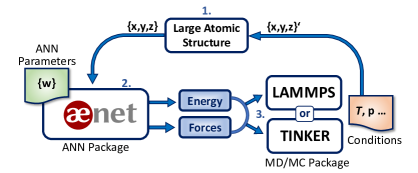
Figure 1: Schematic overview of the ænet-LAMMPS / ænet-TINKER program interfaces for efficient atomistic simulations with artificial neural network (ANN) potentials. The Cartesian coordinates $\bigl{\{}x,y,z\bigr{\}}$ of a large (periodic or non-periodic) atomic system (1) are mapped to total energy and atomic forces by a previously trained ANN potential (2) defined by a set of model parameters $\bigl{\{}w\bigr{\}}$. Via an interface (3) between the open-source ANN code ænet Artrith and Urban (2016), using the ænet library (ænetLib), and the molecular dynamics (MD) / Monte Carlo (MC) codes LAMMPS Plimpton (1995) or TINKER Ponder and Richards (1987), force and/or energy information are used to propagate the initial atomic positions to a new structure with coordinates $\bigl{\{}x,y,z\bigr{\}}^{\prime}$ under a set of specified thermodynamic conditions such as temperature, $T$, and pressure, p. The cycle repeats until a trajectory of sufficient length has been generated from which the properties of interest can be obtained.

The ænet package Artrith and Urban (2016) is a free and open source software for the construction (training) and evaluation of ANN-based machine-learning potentials. ænet implements a variant of the high-dimensional neural network potential method by Behler and Parrinello Behler and Parrinello (2007) described in the previous section II. The cost of computing ænet’s structure descriptors, detailed in section II.2, does not scale with the number of atomic species. This enables the systematic construction of efficient and accurate ANN potentials without manual parametrization for compositions with a large number of atom types Artrith et al. (2017). With the Chebyshev descriptor the cumbersome setup of hand-crafted descriptors is avoided and replaced by just a single line of code in the ænet input.

The ænet package can be compiled into a library (ænetLib) that is compatible with the Python, C/C++, and FORTRAN programming languages, facilitating the integration with simulation software. A Python interface to the Atomic Simulation Environment (ASE) Larsen et al. (2017) is provided in Ref. 19. ASE is a Python framework for atomistic simulations and provides a simple API together with calculators for interfacing with third-party software for the evaluation of structural energies and atomic forces. The ænet package includes an implementation of an ASE calculator linked to ænetLib. A C++ interface to the LAMMPS code is also provided in Ref 25. This interface is designed for the metallurgical analysis in structural materials, such as BCC iron. For example, this interface extends ænetLib so that the stress tensor of the entire system can be calculated using the functionality in LAMMPS Thompson et al. (2009).

In this work, we describe two interfaces with aenetLib coupled to software code written in Fortran and C++: the TINKER and LAMMPS codes, respectively. These simulation software packages are designed with different use cases in mind: TINKER is implemented in the FORTRAN programming language and is structured into small command-line utilities, each with distinct purpose (e.g., MD simulations, geometry optimizations, MC simulations, etc.). From a user perspective, TINKER is comparatively easy to learn and install from source code, which makes it a popular choice for desktop or laptop computers. The standard distribution of TINKER is shared memory parallelized with the Open Multi-Processing (OpenMP) Dagum and Menon (1998) standard, so that simulations can make optimal use of modern consumer-grade processors. LAMMPS, on the other hand, is a highly optimized MD software designed for massively parallel high-performance computer (HPC) systems. LAMMPS input files are scriptable, which adds flexibility but also steepens the learning curve. LAMMPS is distributed-memory parallelized using the message passing interface (MPI) standard and can scale to thousands of distributed processor cores. We note that a TINKER distribution for HPC systems has recently been released, named Tinker-HP Lagardère et al. (2018); Adjoua et al. (2021). Data reported here was, however, obtained with the standard TINKER distribution.

Fig. 1 shows the general workflow for performing efficient atomistic simulations with MLPs: The Cartesian coordinates of an initial atomic structure are mapped to their corresponding total energy and atomic forces via the MLP package ænet given an MLP that is parametrized for all elements in the system. Employing an interface coupling the ænetLib library to either the TINKER or LAMMPS simulation package, the system of interest is propagated to a new set of coordinates under a specified set of thermodynamic conditions. Both LAMMPS and standard TINKER were interfaced with ænet by linking against the ænetLib library, so that ænet routines are used for evaluating structural energies and interatomic forces. In the following section, we describe the implementation and usage of these interfaces.

Note that ænet-TINKER uses the neighbor list from ænet, which is implemented by a comparatively simple algorithm, while ænet-LAMMPS makes direct use of the highly optimized LAMMPS neighbor list.

III.1 Building TINKER with ænet support

Three new files were created to connect the ænet libraries with TINKER: aenettinker.f90, extra.f, and extra1.f.

Using an ANN potential with the TINKER MD code requires to copy the following files to the TINKER source directory,

⬇

1aenettinker.f90

2extra.f

3extra1.f

and to compile the TINKER source code using the provided Makefile, e.g.,

⬇

1Makefile.aenetlib_ifort

2Makefile.aenetlib_gfortran.

III.2 Running TINKER simulations using ænet potentials

To run simulations using ænet ANN potentials, the TINKER parameter file aenet.prm is used. It only contains the masses of all chemical species, as no further information is required.

All ANN potential files have to be present in the working directory and need to follow the naming convention

⬇

1<species>.ann,

where $<$species$>$ is the chemical symbol (H, He, Li, etc.). In the principal TINKER key input file, ænet potentials are activated with the keyword

⬇

1EXTRATERM only.

The number of threads used in parallel runs can be controlled with the keyword OPENMP-THREADS. We refer also to the example Tinker input file tinker.key on our shared repository.

III.3 Building LAMMPS with ænet support

Similar to the TINKER package, two new files,

⬇

1pair_aenet.h

2pair_aenet.cpp,

were written as part of the USER-AENET package to build ænet-LAMMPS by connecting with the ænet libraries.

For building the ænet-LAMMPS interface, the USER-AENET package has to be copied into the LAMMPS source directory and the default Makefile in the LAMMPS source directory needs to be replaced by the one we provide. The user needs to include this package when building LAMMPS by calling,

⬇

1make yes-user-aenet

in the LAMMPS source directory and then compile LAMMPS using the Makefile.

III.4 Running LAMMPS simulations using ænet potentials

The ænet library files, as well as any other dependencies, need to be properly loaded (i.e. by setting the $LD$\_$LIBRARY$\_$PATH). The LAMMPS input script also needs to be configured so as to use the ænet pair style and to specify which neural network parameter (.ann) files to use.

A partial input example for water is provided below:

⬇

1units metal

2mass 1 1.007825

3mass 2 15.999491

4pair_style aenet H.ann O.ann

5pair_coeff * *

The user must specify the order of the $<$species$>$.ann potential files such that they correspond to the mass values defined above. In the example above, element 1 is designated to be hydrogen and element 2 is oxygen. Consequently, the ænet parameter file for hydrogen (H.ann) needs to be specified first and then followed by the parameter file for oxygen (O.ann).

The selected LAMMPS unit system should match the units of the reference data used for training the MLP by ænet. In the example above metal units are used, meaning that the ænet potentials were fitted to training data for which the energies were reported in electron-volts and the positions in Angstroms. If instead the training data is provided in units of Hartrees and Bohrs, then the corresponding LAMMPS unit system electron should be chosen. Further details on the unit systems can be looked up in the LAMMPS manual.

IV Results and Discussion

IV.1 Complex systems require efficient and accurate simulation tools

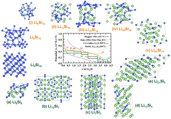
Figure 2: Complex phases of LiSi alloys. Different crystalline and quasi-amorphous Li_xSi structures (color codes: Li$=$green and Si$=$blue) that can occur during the lithiation and delithiation of silicon anodes and exhibit a wide variety of structural motifs and chemical bonds. The relative lithium content x in the amorphous Li_xSi alloys varies during battery charge and discharge (experimental values from Refs. 52 and 53). The structure models were taken from Refs. 35 and 36.

The accurate modeling of complex materials at experimental conditions often requires the use of large simulation cells containing thousands of atoms. Long simulation times on the order of nanoseconds are needed if the dynamics of the systems are of interest. In addition to these efficiency requirements, the complex bonding patterns that govern the atomic interactions need to be described by an appropriate method of sufficient accuracy. MLPs trained to accurate QM calculations can fulfill both the efficiency and the accuracy requirements. Two examples that demonstrate the need for efficient and accurate simulation tools are the transport of Li in nanostructured amorphous Si for high-energy-density batteries and diffusion phenomena in liquid water.

Diffusion in complex amorphous Li_xSi materials: Nanostructured silicon (Si) is a promising alternative to graphite as high-capacity anode material for Li-ion batteries McDowell et al. (2013); Su et al. (2013); Zamfir et al. (2013); Domi et al. (2020, 2021); Cangaz et al. (2020); Cao et al. (2019); Zhu et al. (2019). Nanoscaled materials are required to overcome mechanical limitations and avoid fracturing Wang et al. (2015). In addition, the rate-capability of silicon anodes is 2–4 orders of magnitude lower Ding et al. (2009); Xie et al. (2010); Li et al. (2012) compared to graphite anodes Park et al. (2010) owing to lower Li diffusivity. The lithiation of crystalline Si (c-Si) results in amorphization of the silicon crystal structure McDowell et al. (2013). The amorphous structure of silicon anodes, the length-scale dependence of its mechanical properties, and the comparatively low lithium conductivity make the investigation of lithium transport in silicon electrodes challenging for computation and experiment. We have previously employed ANN potentials to investigate the complex phase diagram of amorphous LiSi alloys Artrith et al. (2018) and the delithiation of entire Li_xSi nanoparticles Artrith et al. (2019). Fig. 2 shows examples of different crystalline and quasi-amorphous Li_xSi structures that can occur during the lithiation and delithiation of silicon anodes, which exhibit a wide variety of structural motifs and chemical bonds.

These considerations make this system a prototypical complex material that cannot easily be modeled with either first principles methods or conventional interatomic potentials but can be successfully described by ANN potentials Artrith et al. (2018, 2019).

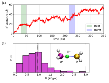
Figure 3: Importance of long-time simulations for predicting proton defect diffusion. (a) The diffusion process of a hydronium ($H_{3}O^{+}$) defect in liquid water, shown as the distance of the defect position at time $t_{i}$ from its position at time $t_{0}$, is characterized by alternating periods of rapid defect movement (burst phase highlighted in blue) and little change in position ($rest$ phase highlighted in green) which can extend over 10s of picoseconds. (b) Defect diffusion coefficients obtained from 20 picosecond segments extracted from the 350 ps trajectory shown in (a) are distributed across a large value range indicating that a single trajectory of that length is insufficient to estimate the proton defect diffusion coefficient. Results from periodic AIMD simulations containing 63 H2O molecules and a single H3O defect. Napoli et al. (2018)

Diffusion in liquid water: The need for efficient simulation tools coupled to MLPs becomes also apparent when studying diffusion phenomena in complex molecular systems. One example is the transport of proton defectsVoth (2006); Marx et al. (2010), a crucial process for the understanding of electrochemical reactions and enzymatic mechanisms that requires a simulation method with the ability to break and form chemical bonds. Ab initio molecular dynamics (AIMD) simulations are in principle able to describe the diffusion of protons in hydrogen-bond networks but are limited to short time-scales and often neglect nuclear quantum effectsMarkland and Ceriotti (2018). As demonstrated in Fig. 3 short simulations with a length of 10s of picoseconds are not sufficient to reliably obtain proton defect diffusion coefficients in liquid water. This is a consequence of the Grotthuss mechanism in which structural diffusion occurs in a stepwise fashion with periods of rapid defect diffusion followed by rest states with little movement Hassanali et al. (2013); Tse et al. (2015) that makes it necessary to follow the defect trajectories over several nanoseconds. The issue is further complicated by the fact that periodic simulation cells are usually small in size to save computing resources and therefore often contain only a single defect. Even when averaging over multiple atoms is possible, as in case of molecular diffusion in pure liquid water, an accurate prediction and comparison to the experimentally observed property is not straightforward. While structural properties of liquid water such as pair distribution functions can be routinely obtained from direct AIMD simulations employing relatively small simulation cells and moderate simulation times, dynamical properties are more challenging since they have a strong system size dependence and require longer times to converge Kühne et al. (2009).

As these two examples demonstrate, efficient tools to generate long trajectories for complex atomistic system are a prerequisite for obtaining reliable molecular and materials properties. In the next section we show how the ænet-TINKER and ænet-LAMMPS interfaces can meet these requirements while making efficient use of modern compute hardware distributing compute load across CPUs.

We demonstrate the computational efficiency of the combination of MLPs with the MD codes TINKER (Fig. 4) and LAMMPS (Fig. 5) for amorphous LiSi and bulk water with simulation cells of increasing size containing up to millions of atoms. ANN potentials for both systems trained to publicly available datasets Chen et al. (2020) are provided with the implementation together with the corresponding input files and reference output to facilitate a quick set up of the simulation and guarantee reproducibility Artrith et al. (2021). In brief, these ANNs are trained to reference DFT calculations, for LiSi with the PBE Perdew et al. (1996) density-functional on data covering bulk, surface, and cluster structures at various LiSi compositions, see details in Refs. 35 and 36. The liquid water ANN was trained on liquid water structures across the full liquid temperature range described by the revPBE-D3 Perdew et al. (1996); Zhang and Yang (1998); Grimme et al. (2010) density-functional. We have previously shown that an ANN potential trained to this same dataset with a different set of descriptors yields accurate results across the full liquid temperature range Morawietz et al. (2018). A recent study also found that local environments sampled in liquid water are sufficiently similar to the environments in different ice phases that an MLP trained on only liquid water configurations is able reproduce many properties of ice Monserrat et al. (2020). For details on the availability of potentials and data sets see section Data Availability.

IV.2 Performance of ænet-TINKER and ænet-LAMMPS interfaces

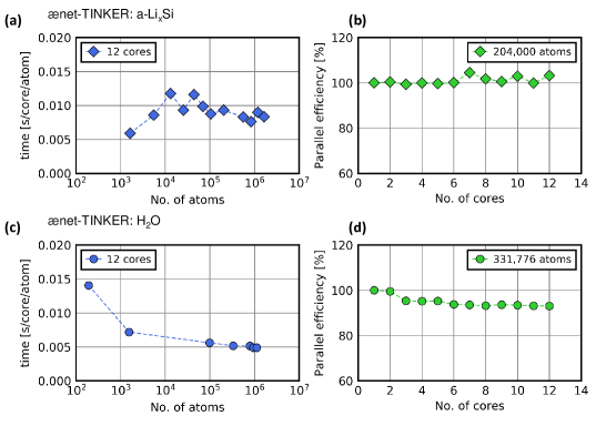
Figure 4: Computational efficiency of molecular dynamics simulations with the ænet-TINKER interface. (a-b) a-LiSi and (c-d) water. Computer cluster specifications: Dell C6420 nodes with dual Intel Xeon Gold 6126 Processor (2.6 Ghz) with Intel compiler 2017, EDR Infiniband, Red Hat Enterprise Linux 7.

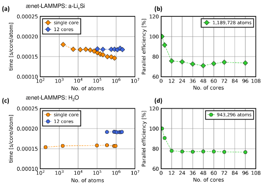
Figure 5: Computational efficiency of molecular dynamics simulations with the ænet-LAMMPS interface. (a-b) a-LiSi and (c-d) water. Computer cluster specifications: Dell C6420 nodes with dual Intel Xeon Gold 6126 Processor (2.6 Ghz) with Intel compiler 2017, EDR Infiniband, Red Hat Enterprise Linux 7.

A major drawback of direct AIMD simulations is their steep increase in compute time with the number of atoms in the system. Common DFT calculations have an algorithmic scaling of order $\mathcal{O}(N^{3})$ or $\mathcal{O}(N\log{}N)$ with the number of electrons $N$ in the system.

To demonstrate the impact of system size on compute cost for our MLP-based simulation interfaces we compare the compute time per atom for periodic simulation cells of crystalline LiSi, panel (a) of Figs. 4-5, and bulk H₂O, panel (c) of Figs. 4-5, ranging from a few hundred atoms all the way up to millions of atoms. All scaling tests were performed on the Columbia HPC cluster Terremoto, using Dell C6420 nodes (24 cores per node) with dual Intel Xeon Gold 6126 Processors (2.6 Ghz) using the Intel 2017 compiler, EDR Infiniband, and Red Hat Enterprise Linux 7.

As can be seen from the results in Figs. 4-5 computational costs for both interfaces scale strictly linearly with system size, even up to very large unit cells, which is a result of the employed ANN approach in which the total atomic interactions are represented by local, atom-centered ANNs Behler and Parrinello (2007); Artrith and Urban (2016). Even though we evaluate performance on two very different systems (an amorphous solid and a molecular liquid) both display very similar compute requirements, with single core compute times per atoms of $\sim$10 milliseconds with TINKER (Fig. 4) and $<$ 1 millisecond for LAMMPS (Fig. 5). As discussed, the current TINKER interface is based on the original implementation making use of OpenMP parallelization. Even higher efficiency can be expected with the recently released TINKER-HP package Lagardère et al. (2018). To translate these numbers into compute times: to generate a 1 ns-long trajectory of a system of 1536 atoms (for H₂O) takes 134 h on a single compute core with ænet-LAMMPS.

We note that the overall efficiency difference of the ænet-TINKER and ænet-LAMMPS interfaces is mainly due to the evaluation of the particle neighbor lists that are used to determined which atoms are in the local atomic environment of each atom. The ænet-TINKER interface currently uses the neighbor list implemented in ænet, which is not optimized for MD simulations and is rebuilt at each step of the simulation. In contrast, the ænet-LAMMPS interface makes use of LAMMPS’ highly optimized neighbor list implementation, which can reduce the computational cost for MD simulations significantly for large atomic structures.

To further reduce the wait time the compute load can be distributed across cores. In panels (b,d) of Figs. 4- 5 we report the parallel efficiency, i.e. the loss of compute power due to the distribution of tasks and the communication between the compute cores. Due to OpenMP parallelization the ænet-TINKER simulations (Fig. 4) have an efficiency very close to 100% on a single node. For ænet-LAMMPS (Fig. 5) efficiency drops more but still stays at high values of around 70-80% using up to 96 CPU cores on multiple nodes and with an overall better efficiency than the ænet-TINKER interface. Parallelization over multiple cores reduces the real wait time for our example system of 1536 atom to 3.6 h on 48 cores and just 1.8 h on 96 cores.

Apart from size and composition of the system of interest, the simulation performance is also dependent on the specifications of the ANN potential which in turn has a direct impact on the accuracy of the calculated properties. In contrast to other MLP approaches, such as Gaussian Approximation Potentials Bartók et al. (2010), the efficiency of ANN-based models does not depend on the size of the training dataset since the parameters that determine the potentials are only optimized once before the simulation. For ANN potentials a main factor that determines both simulation efficiency and accuracy is the complexity of the model as defined by the number of nodes per layer. The size of the input layer is given by the number of descriptors while the hidden layer size is a separate hyperparameter that has to be tuned during model construction.

To investigate these effects and provide guidance for the construction of new ANN potentials we have trained two additional potentials for water with gradually decreased complexity. The optimal ANN potential model that was used for benchmarking the computational efficiency in Figs. 4 and 5 and the diffusion analysis shown in the following section has a 52-25-25-1 architecture. First, the size of the descriptor was reduced from 52 to 20 dimensions and then, in addition, the hidden layer width was decreased from 25 to 5, i.e., the architecture was reduced to 20-25-25-1 and 20-5-5-1, respectively. In Fig. 6 the performance of the reduced models is compared to the optimal model (52-25-25-1) as a default.

As can be seen, the descriptor size is a major factor determining model accuracy (Fig. 6a–e) and simulation speed (Fig. 6f). While cutting the descriptor leads to a simulation speed-up of a factor of 3 (Fig. 6f), the energy and force accuracy decreases (Fig. 6a–b) and deviations in dynamics properties become visible. Although, the structural properties (as exemplified by the oxygen-oxygen RDF) show only a low variance across models (Fig. 6c), the reduced model shows a broadening and shift of the OH bending region of the hydrogen vibrational density of states (VDOS, Fig. 6d). Further simplifying the ANN potential by reducing the hidden layer width only marginally improves the efficiency but results in greater deviations of the VDOS now also effecting the OH stretch region.

In the following, we directly demonstrate the impact of the two efficient simulation interfaces: making use of ænet-TINKER to equilibrate a large nanoparticle of LiSi and using ænet-LAMMPS to calculate the liquid water diffusivity at experimental conditions.

IV.3 ænet-TINKER applied to LiSi

To demonstrate the feasibility of large-scale simulations of nanostructures, we performed an MD equilibration simulation of a Li_xSi nanoparticle with 11,000 atoms (8 nm diameter) at 500 K using the ænet-TINKER interface. The initial structure (truncated from the Li15Si4 crystal structure), and the final equilibrated structure are shown in Fig. 7. The progression of the potential energy during the MD simulation and its gliding average over 10 ps is illustrated in Fig. 8. After around 2 ns the potential energy is within 2 meV/atom of the final structure, indicating that the system has reached thermal equilibrium. This example further illustrates the need for efficient long-time MD simulations to investigate the properties of LiSi anodesArtrith et al. (2018, 2019).

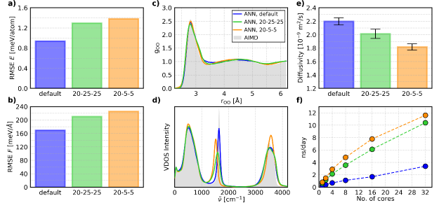
Figure 6: Impact of model complexity on accuracy and simulation efficiency. (a-b) Test set accuracy of energies (panel a) and forces (panel b) for three ANN potentials with decreasing model complexity (specified as [number of input nodes] – [number of nodes in hidden layer 1] – [number of nodes in hidden layer 2]; default model complexity: 52-25-25). (c-d) Oxygen-oxygen radial distribution functions (panel c) and vibrational density of states (VDOS) of the hydrogen atoms (panel d) compared to results from direct AIMD simulations Marsalek and Markland (2017). (e) System-size dependent diffusion coefficients, $D(L)$, at a box size of 64 H2O molecules. (f) Simulation time in nanoseconds accumulated on one day of compute as a function of the number of employed cores.

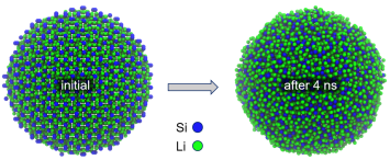
Figure 7: LiSi nanoparticle equilibrated with the ænet-TINKER interface. Molecular dynamics (MD) simulation of a Li₈₄₂₉Si₂₅₇₁ nanoparticle structure (11,000 atoms, diameter 8 nm). Left: initial structure before MD; right: final structure after 4 ns MD simulation.

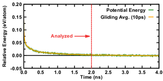
Figure 8: Equilibration of a LiSi nanoparticle with the ænet-TINKER interface. The amorphous LiSi nanoparticle structure (11,000 atoms, structure shown in Fig. 7) has reached thermal equilibrium after 2 ns long molecular dynamics (MD) simulations at 500 K. The MD trajectory was used to analyze properties between 2 - 4 ns. Gliding average (10 ps) of the potential energy during MD simulation of the nanoparticle model with composition Li₈₄₂₉Si₂₅₇₁ at 500 K.

IV.4 ænet-LAMMPS applied to H₂O

As an additional demonstration of the benefits of an efficient, linear scaling MD setup for ab initio-quality simulations we report results on molecular diffusion in liquid water employing the ænet-LAMMPS interface. Diffusion coefficients were calculated from the mean square displacement of the oxygen positions

$$D=\lim_{t\rightarrow\infty}\frac{1}{6}\frac{d}{dt}\left<\left|r(t)-r(0)\right|^{2}\right>\quad.$$ (10)

As discussed above the accurate prediction of dynamic properties such as diffusion coefficients is particularly challenging due to their system size dependence resulting from hydrodynamic interactions Dünweg and Kremer (1993). For the small system sizes still affordable by direct AIMD this can lead do deviations between the diffusion coefficient computed at finite system size and the infinite-system limit that should be compared to the experiment Yeh and Hummer (2004). A common solution is to apply a correction formula that extrapolates the diffusion coefficient at finite system size, $D\bigl{(}L\bigr{)}$, to the infinite system size limit,

$$D\bigl{(}\infty\bigr{)}=D\bigl{(}L\bigr{)}+\frac{\xi}{6\pi\beta}\frac{1}{\eta L},$$ (11)

with $\beta=(k_{\text{B}}T)^{-1}$, the length of the cubic simulation cell $L$, the shear viscosity $\eta$, and a constant $\xi$ $=$ 2.837297 Dünweg and Kremer (1993); Yeh and Hummer (2004). However this formula requires a value for the viscosity which is often taken from experiment and might not correspond to the value one would obtain from simulations with a particular computational method (density-functional, interatomic potential, or force field).

Using the ænet-LAMMPS interface we performed MD simulations with increasingly larger simulation cells (containing up to 3072 atoms with a total time of 1 ns per system) to estimate the diffusion coefficient of liquid water at experimental conditions. As shown in Fig. 9 the size-independent diffusion coefficient $D\bigl{(}\infty\bigr{)}$ that should be compared to experiment is obtained directly by extrapolating the diffusivity obtained from finite simulation cells to infinite system size employing the linear relationship between diffusion and inverse box length. Compared to the estimate obtained with the correction formula, Eq. 11, the $D\bigl{(}\infty\bigr{)}$ value from direct extrapolation (line fit to $D(L)$ vs. $1/L$) is lower, indicating that the viscosity of revPBE-based ANN water is higher than the experimental one at 300 K.

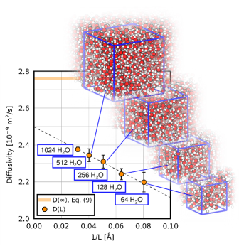
Figure 9: Calculation of the liquid water diffusivity with the ænet-LAMMPS interface. Liquid water diffusion coefficients as function of the inverse length of the simulation cell, $1/L$, (shown as orange circle) obtained from ANN simulations with increasingly larger simulations cells. Error bars represent the standard error of the mean from a set of diffusion coefficients obtained from five independent runs (of length 200 ps each) per system size. Extrapolation to infinite system size employing the linear relationship between diffusion and inverse box length yields an estimate of the diffusion coefficient at experimental conditions $D(\infty)=2.5\times{}10^{-9}$ m²/s (dashed line at $1/L=0.0$). A corrected diffusion coefficient based on the ANN results for 64 H2O obtained with the correction formula of Eq. 11 using the experimental viscosity value is displayed as orange shaded line.

V Conclusion

To realize the full potential of machine learning accelerated atomistic simulations, MLPs need to be made compatible with existing highly optimized simulation software. Here, we reported interfaces of the ænet ANN potential software with the LAMMPS and TINKER simulation packages for accurate and efficient simulations of complex atomic systems. We detailed the installation and usage and discussed implementation differences. Both interfaces facilitate large-scale molecular dynamics simulations on modern parallel computer architectures with single step compute times of (sub-)milliseconds for both systems, an amorphous material and a molecular liquid. The shared-memory parallelized ænet-TINKER interface shows nearly perfect parallel efficiency on a single computer node. The distributed-memory parallelized ænet-LAMMPS interface scales with excellent efficiency ($\sim$80%) on multi-node architectures as tested here with up to $\sim$100 computer cores. The ænet-LAMMPS interface further shows generally a higher efficiency than the ænet-TINKER interface owing to the highly optimized neighbor list implementation in LAMMPS. The ænet-TINKER currently uses ænet’s internal neighbor list that is not optimized for MD simulations, and the efficiency of the interface for large structures could be further improved by making use of TINKER’s own implementation. Both interfaces make it possible to simulate atomic structures with several hundreds of thousands to millions of atoms with an accuracy close to first principles calculations. Further improvement in the efficiency of such simulations can be expected in the future when support for graphical processor units (GPUs) becomes available.

Data availability

DFT reference data: The reference datasets of the crystalline/amorphous LiSi and liquid water systems can be obtained from the Materials Cloud repository (https://doi.org/10.24435/materialscloud:dx-ct). These datasets contain atomic structures and interatomic forces in the XCrySDen Kokalj (Aug) structure format (XSF), and total energies are included as additional meta information.

Code availability: The ænet source code and its documentation can be obtained either from the ænet website (http://ann.atomistic.net) or from GitHub (https://github.com/atomisticnet/aenet). The implementation and examples including ANN potentials for crystalline/amorphous LiSi and liquid water can be found here: 1. ænet-LAMMPS code (https://github.com/atomisticnet/aenet-lammps); 2. ænet-TINKER code (https://github.com/atomisticnet/aenet-tinker).

Tutorials: Jupyter notebooks with tutorials demonstrating the usage of the TINKER and LAMMPS interfaces for three different example systems can be found at:

• ænet-tinker (amorphous LiSi): https://github.com/atomisticnet/aenet-tinker/tree/master/tutorial;

• ænet-lammps (liquid bulk water): https://github.com/atomisticnet/aenet-lammps/tree/master/tutorial;

• ænet-lammps (BCC iron): https://github.com/HidekiMori-CIT/aenet-lammps/tree/master/tutorial.

References

- Frenkel and Smit (2001) D. Frenkel and B. Smit, Understanding Molecular Simulation: From Algorithms to Applications (Elsevier, 2001).
- Allen and Tildesley (2017) M. P. Allen and D. J. Tildesley, Computer Simulation of Liquids (Oxford University Press, 2017).
- Curtarolo et al. (2013) S. Curtarolo, G. L. W. Hart, M. B. Nardelli, N. Mingo, S. Sanvito, and O. Levy, Nature Materials 12, 191 (2013).
- Jain et al. (2016) A. Jain, Y. Shin, and K. A. Persson, Nature Reviews Materials 1, 1 (2016).
- Urban et al. (2016) A. Urban, D.-H. Seo, and G. Ceder, npj Computational Materials 2, 1 (2016).
- Seh et al. (2017) Z. W. Seh, J. Kibsgaard, C. F. Dickens, I. Chorkendorff, J. K. Nørskov, and T. F. Jaramillo, Science 355 (2017), 10.1126/science.aad4998.
- Oganov et al. (2019) A. R. Oganov, C. J. Pickard, Q. Zhu, and R. J. Needs, Nature Reviews Materials 4, 331 (2019).
- Jorgensen (2004) W. L. Jorgensen, Science 303, 1813 (2004).
- Van Drie (2007) J. H. Van Drie, Journal of Computer-Aided Molecular Design 21, 591 (2007).
- Aminpour et al. (2019) M. Aminpour, C. Montemagno, and J. A. Tuszynski, Molecules 24, 1693 (2019).
- Morawietz and Artrith (2020) T. Morawietz and N. Artrith, Journal of Computer-Aided Molecular Design (2020), 10.1007/s10822-020-00346-6.
- Becker et al. (2013) C. A. Becker, F. Tavazza, Z. T. Trautt, and R. A. Buarque de Macedo, Current Opinion in Solid State and Materials Science Frontiers in Methods for Materials Simulations, 17, 277 (2013).
- Jorgensen and Tirado-Rives (2005) W. L. Jorgensen and J. Tirado-Rives, Proceedings of the National Academy of Sciences 102, 6665 (2005).
- Behler and Parrinello (2007) J. Behler and M. Parrinello, Physical Review Letters 98, 146401 (2007).
- Bartók et al. (2010) A. P. Bartók, M. C. Payne, R. Kondor, and G. Csányi, Physical Review Letters 104, 136403 (2010).
- Artrith et al. (2011) N. Artrith, T. Morawietz, and J. Behler, Physical Review B 83 (2011), 10.1103/PhysRevB.83.153101.
- Jose et al. (2012) K. V. J. Jose, N. Artrith, and J. Behler, The Journal of Chemical Physics 136, 194111 (2012).
- Botu and Ramprasad (2015) V. Botu and R. Ramprasad, International Journal of Quantum Chemistry 115, 1074 (2015).
- Artrith and Urban (2016) N. Artrith and A. Urban, Computational Materials Science 114, 135 (2016).
- Shapeev (2016) A. V. Shapeev, Multiscale Modeling & Simulation 14, 1153 (2016).
- Khorshidi and Peterson (2016) A. Khorshidi and A. A. Peterson, Computer Physics Communications 207, 310 (2016).
- S. Smith et al. (2017) J. S. Smith, O. Isayev, and A. E. Roitberg, Chemical Science 8, 3192 (2017).
- Unke and Meuwly (2018) O. T. Unke and M. Meuwly, The Journal of Chemical Physics 148, 241708 (2018).
- Schütt et al. (2018) K. T. Schütt, H. E. Sauceda, P.-J. Kindermans, A. Tkatchenko, and K.-R. Müller, The Journal of Chemical Physics 148, 241722 (2018).
- Mori and Ozaki (2020) H. Mori and T. Ozaki, Physical Review Materials 4, 040601 (2020).
- Miksch et al. (2021) A. M. Miksch, T. Morawietz, J. Kästner, A. Urban, and N. Artrith, Machine Learning: Science and Technology (2021), 10.1088/2632-2153/abfd96.
- Burke (2012) K. Burke, The Journal of Chemical Physics 136, 150901 (2012).
- Artrith et al. (2013) N. Artrith, B. Hiller, and J. Behler, physica status solidi (b) 250, 1191 (2013).
- Artrith (2019) N. Artrith, Journal of Physics: Energy 1, 032002 (2019).
- Mueller et al. (2020) T. Mueller, A. Hernandez, and C. Wang, The Journal of Chemical Physics 152, 050902 (2020).
- Ponder and Richards (1987) J. W. Ponder and F. M. Richards, Journal of Computational Chemistry 8, 1016 (1987).
- Plimpton (1995) S. Plimpton, Journal of Computational Physics 117, 1 (1995).
- Thompson et al. (2015) A. P. Thompson, L. P. Swiler, C. R. Trott, S. M. Foiles, and G. J. Tucker, Journal of Computational Physics 285, 316 (2015).
- Zuo et al. (2020) Y. Zuo, C. Chen, X. Li, Z. Deng, Y. Chen, J. Behler, G. Csányi, A. V. Shapeev, A. P. Thompson, M. A. Wood, and S. P. Ong, The Journal of Physical Chemistry A 124, 731 (2020).
- Artrith et al. (2018) N. Artrith, A. Urban, and G. Ceder, The Journal of Chemical Physics 148, 241711 (2018).
- Artrith et al. (2019) N. Artrith, A. Urban, Y. Wang, and G. Ceder, arXiv:1901.09272 [cond-mat, physics:physics] (2019), arXiv:1901.09272 [cond-mat, physics:physics] .
- Morawietz et al. (2018) T. Morawietz, O. Marsalek, S. R. Pattenaude, L. M. Streacker, D. Ben-Amotz, and T. E. Markland, The Journal of Physical Chemistry Letters 9, 851 (2018).
- Morawietz et al. (2019) T. Morawietz, A. S. Urbina, P. K. Wise, X. Wu, W. Lu, D. Ben-Amotz, and T. E. Markland, The Journal of Physical Chemistry Letters 10, 6067 (2019).
- Cybenko (1989) G. Cybenko, Mathematics of Control, Signals, and Systems 2, 303 (1989).
- Artrith et al. (2017) N. Artrith, A. Urban, and G. Ceder, Physical Review B 96 (2017), 10.1103/PhysRevB.96.014112.
- Broyden (1970) C. G. Broyden, IMA Journal of Applied Mathematics 6, 76 (1970).
- Fletcher (1970) R. Fletcher, Comput. J. 13, 317 (1970).
- Goldfarb (1970) D. Goldfarb, Math. Comp. 24, 23 (1970).
- Shanno (1970) D. F. Shanno, Math. Comp. 24, 647 (1970).
- Liu and Nocedal (1989) D. C. Liu and J. Nocedal, Math. Program. 45, 503 (1989).
- LeCun et al. (2012) Y. A. LeCun, L. Bottou, G. B. Orr, and K.-R. Müller, “Efficient backprop,” in Neural Networks: Tricks of the Trade: Second Edition, edited by G. Montavon, G. B. Orr, and K.-R. Müller (Springer Berlin Heidelberg, Berlin, Heidelberg, 2012) pp. 9–48.
- Larsen et al. (2017) A. H. Larsen, J. J. Mortensen, J. Blomqvist, I. E. Castelli, R. Christensen, M. Du\lak, J. Friis, M. N. Groves, B. Hammer, C. Hargus, E. D. Hermes, P. C. Jennings, P. B. Jensen, J. Kermode, J. R. Kitchin, E. L. Kolsbjerg, J. Kubal, K. Kaasbjerg, S. Lysgaard, J. B. Maronsson, T. Maxson, T. Olsen, L. Pastewka, A. Peterson, C. Rostgaard, J. Schiøtz, O. Schütt, M. Strange, K. S. Thygesen, T. Vegge, L. Vilhelmsen, M. Walter, Z. Zeng, and K. W. Jacobsen, Journal of Physics: Condensed Matter 29, 273002 (2017).
- Thompson et al. (2009) A. P. Thompson, S. J. Plimpton, and W. Mattson, The Journal of chemical physics 131, 154107 (2009).
- Dagum and Menon (1998) L. Dagum and R. Menon, IEEE Computational Science and Engineering 5, 46 (1998).
- Lagardère et al. (2018) L. Lagardère, L.-H. Jolly, F. Lipparini, F. Aviat, B. Stamm, Z. F. Jing, M. Harger, H. Torabifard, G. Andrés Cisneros, M. J. Schnieders, N. Gresh, Y. Maday, P. Y. Ren, J. W. Ponder, and J.-P. Piquemal, Chemical Science 9, 956 (2018).
- Adjoua et al. (2021) O. Adjoua, L. Lagardère, L.-H. Jolly, A. Durocher, T. Very, I. Dupays, Z. Wang, T. J. Inizan, F. Célerse, P. Ren, J. W. Ponder, and J.-P. Piquemal, arXiv:2011.01207 [physics] (2021), arXiv:2011.01207 [physics] .
- Wen and Huggins (1981) C. J. Wen and R. A. Huggins, Journal of Solid State Chemistry 37, 271 (1981).
- Hatchard and Dahn (2004) T. D. Hatchard and J. R. Dahn, Journal of The Electrochemical Society 151, A838 (2004).
- McDowell et al. (2013) M. T. McDowell, S. W. Lee, W. D. Nix, and Y. Cui, Adv. Mater. 25, 4966 (2013).
- Su et al. (2013) X. Su, Q. Wu, J. Li, X. Xiao, A. Lott, W. Lu, B. W. Sheldon, and J. Wu, Adv. Energy Mater. 4 (2013), 10.1002/aenm.201300882.
- Zamfir et al. (2013) M. R. Zamfir, H. T. Nguyen, E. Moyen, Y. H. Lee, and D. Pribat, J. Mater. Chem. A 1, 9566 (2013).
- Domi et al. (2020) Y. Domi, H. Usui, A. Ando, K. Nishikawa, and H. Sakaguchi, ACS Applied Energy Materials 3, 8619 (2020).
- Domi et al. (2021) Y. Domi, H. Usui, N. Ieuji, K. Nishikawa, and H. Sakaguchi, ACS Applied Materials & Interfaces 13, 3816 (2021).
- Cangaz et al. (2020) S. Cangaz, F. Hippauf, F. S. Reuter, S. Doerfler, T. Abendroth, H. Althues, and S. Kaskel, Advanced Energy Materials 10, 2001320 (2020).
- Cao et al. (2019) C. Cao, I. I. Abate, E. Sivonxay, B. Shyam, C. Jia, B. Moritz, T. P. Devereaux, K. A. Persson, H.-G. Steinrück, and M. F. Toney, Joule 3, 762 (2019).
- Zhu et al. (2019) B. Zhu, G. Liu, G. Lv, Y. Mu, Y. Zhao, Y. Wang, X. Li, P. Yao, Y. Deng, Y. Cui, and J. Zhu, Science Advances 5, eaax0651 (2019).
- Wang et al. (2015) B. Wang, X. Li, B. Luo, L. Hao, M. Zhou, X. Zhang, Z. Fan, and L. Zhi, Adv. Mater. 27, 1526 (2015).
- Ding et al. (2009) N. Ding, J. Xu, Y. Yao, G. Wegner, X. Fang, C. Chen, and I. Lieberwirth, Solid State Ionics 180, 222 (2009).
- Xie et al. (2010) J. Xie, N. Imanishi, T. Zhang, A. Hirano, Y. Takeda, and O. Yamamoto, Mater. Chem. Phys. 120, 421 (2010).
- Li et al. (2012) J. Li, X. Xiao, F. Yang, M. W. Verbrugge, and Y.-T. Cheng, J. Phys. Chem. C 116, 1472 (2012).
- Park et al. (2010) M. Park, X. Zhang, M. Chung, G. B. Less, and A. M. Sastry, J. Power Sources 195, 7904 (2010).
- Napoli et al. (2018) J. A. Napoli, O. Marsalek, and T. E. Markland, The Journal of Chemical Physics 148, 222833 (2018).
- Voth (2006) G. A. Voth, Accounts of Chemical Research 39, 143 (2006).
- Marx et al. (2010) D. Marx, A. Chandra, and M. E. Tuckerman, Chemical Reviews 110, 2174 (2010).
- Markland and Ceriotti (2018) T. E. Markland and M. Ceriotti, Nature Reviews Chemistry 2, 1 (2018).
- Hassanali et al. (2013) A. Hassanali, F. Giberti, J. Cuny, T. D. Kühne, and M. Parrinello, Proceedings of the National Academy of Sciences 110, 13723 (2013).
- Tse et al. (2015) Y.-L. S. Tse, C. Knight, and G. A. Voth, The Journal of Chemical Physics 142, 014104 (2015).
- Kühne et al. (2009) T. D. Kühne, M. Krack, and M. Parrinello, Journal of Chemical Theory and Computation 5, 235 (2009).
- Chen et al. (2020) M. S. Chen, T. Morawietz, T. E. Markland, and N. Artrith, Materials Cloud Archive 2020.92 (2020), doi.org/10.24435/materialscloud:dx-ct.
- Artrith et al. (2021) N. Artrith, K. T. Butler, F.-X. Coudert, S. Han, O. Isayev, A. Jain, and A. Walsh, Nature Chemistry 13, 505 (2021).
- Perdew et al. (1996) J. P. Perdew, K. Burke, and M. Ernzerhof, Physical Review Letters 77, 3865 (1996).
- Zhang and Yang (1998) Y. Zhang and W. Yang, Physical Review Letters 80, 890 (1998).
- Grimme et al. (2010) S. Grimme, J. Antony, S. Ehrlich, and H. Krieg, The Journal of Chemical Physics 132, 154104 (2010).
- Monserrat et al. (2020) B. Monserrat, J. G. Brandenburg, E. A. Engel, and B. Cheng, Nature Communications 11, 5757 (2020).
- Marsalek and Markland (2017) O. Marsalek and T. E. Markland, The Journal of Physical Chemistry Letters 8, 1545 (2017).
- Dünweg and Kremer (1993) B. Dünweg and K. Kremer, The Journal of Chemical Physics 99, 6983 (1993).
- Yeh and Hummer (2004) I.-C. Yeh and G. Hummer, The Journal of Physical Chemistry B 108, 15873 (2004).
- Kokalj ( Aug) A. Kokalj, Journal of Molecular Graphics & Modelling 17, 176 (1999 Jun-Aug).