Human Pose Regression with Residual Log-likelihood Estimation

Abstract

Heatmap-based methods dominate in the field of human pose estimation by modelling the output distribution through likelihood heatmaps. In contrast, regression-based methods are more efficient but suffer from inferior performance. In this work, we explore maximum likelihood estimation (MLE) to develop an efficient and effective regression-based methods. From the perspective of MLE, adopting different regression losses is making different assumptions about the output density function. A density function closer to the true distribution leads to a better regression performance. In light of this, we propose a novel regression paradigm with Residual Log-likelihood Estimation (RLE) to capture the underlying output distribution. Concretely, RLE learns the change of the distribution instead of the unreferenced underlying distribution to facilitate the training process. With the proposed reparameterization design, our method is compatible with off-the-shelf flow models. The proposed method is effective, efficient and flexible. We show its potential in various human pose estimation tasks with comprehensive experiments. Compared to the conventional regression paradigm, regression with RLE bring 12.4 mAP improvement on MSCOCO without any test-time overhead. Moreover, for the first time, especially on multi-person pose estimation, our regression method is superior to the heatmap-based methods. Our code is available at https://github.com/Jeff-sjtu/res-loglikelihood-regression.

1 Introduction

Human pose estimation has been extensively studied in the area of computer vision [23, 24, 1, 32, 21]. Recently, with deep convolutional neural networks, significant progress has been achieved. Existing methods can be divided into two categories: heatmap-based [60, 59, 65, 4, 67, 57, 49, 55] and regression-based [61, 5, 56, 73, 45, 64]. Heatmap-based methods are dominant in the field of human pose estimation. These methods generate a likelihood heatmap for each joint and locate the joint as the point with the argmax [59, 67, 49] or soft-argmax [43, 34, 57] operations. Despite the excellent performance, heatmap-based methods suffer from high computation and storage demands. Expanding the heatmap to 3D or 4D (spatial + temporal) will be costly. Additionally, it is hard to deploy heatmap in modern one-stage methods.

Regression-based methods directly map the input to the output joints coordinates, which is flexible and efficient for various human pose estimation tasks and real-time applications, especially on edge devices. A standard heatmap head (3 deconv layers) costs 1.4$\times$ FLOPs of the ResNet-50 backbone, while the regression head costs only 1/20000 FLOPs of the same backbone. Nevertheless, regression suffer from inferior performance. In challenging cases like occlusions, motion blur, and truncations, the ground-truth labels are inherently ambiguous. Heatmap-based methods are robust to these ambiguities by leveraging the likelihood heatmap. But current regression methods are vulnerable to these noisy labels.

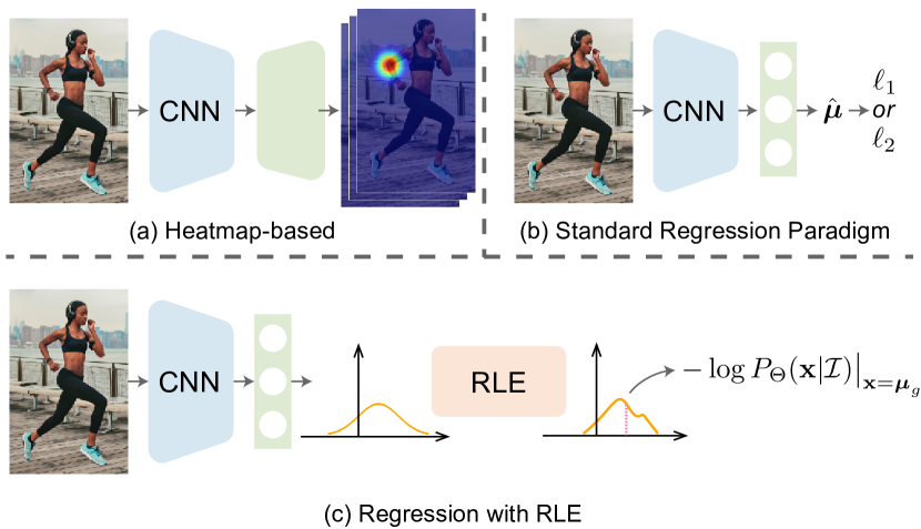
Figure 1: Illustrasion of (a) heatmap-based method, (b) standard regression paradigm, and (c) regression with the proposed RLE.

In this work, we facilitate human pose regression by exploring maximum likelihood estimation (MLE) to model the output distribution. From the perspective of MLE, standard Euclidean distance loss ($\ell_{1}$ or $\ell_{2}$) can be viewed as a particular assumption that the output conforms to a distribution family (Laplace or Gaussian distribution) with constant variance. Intuitively, the regression performance can be improved if we construct the likelihood function with the true underlying distribution instead of the inappropriate hypothesis.

To this end, we propose a novel and effective regression paradigm, named Residual Log-likelihood Estimation (RLE), that leverages normalizing flows to estimate the underlying distribution and boosts human pose regression. Given a tractable preset assumption of the likelihood function, RLE estimates the residual log-likelihood, i.e. the change of the distribution. It is easier to be optimized compared to the original unreferenced underlying distribution. Besides, we design a reparameterization strategy for the flow model to learn the intrinsic characteristics of the underlying distribution. This strategy makes our regression framework feasible and allows us to utilize the off-the-shelf flow model to approximate the distribution without a sophisticated network architecture.

During training, the regression model and the RLE module can be optimized simultaneously. Since the form of the underlying distribution is unknown, the RLE module is also trained via the maximum likelihood estimation process. Besides, the RLE module does not participate in the inference phase. In other words, the proposed method can bring significant improvement to the regression model without any test-time overhead.

The proposed regression framework is general. It can be applied to various human pose estimation algorithms (e.g. two-stage approaches [48, 15, 13, 67, 55], one-stage approaches [73, 45, 64]) and various tasks (e.g. single and multi-person 2D/3D pose estimation [1, 32, 21, 38, 23, 24]). We benchmark the proposed method on three pose estimation datasets, including MPII [1], MSCOCO [32] and Human3.6M [21]. With a simple yet effective architecture, RLE boosts the conventional regression method by 12.4 mAP and achieves superior performance to the heatmap-based methods. Moreover, it is more computation and storage efficient than heatmap-based methods. Specifically, on the MSCOCO dataset [32], our regression-based model with ResNet-50 [16] backbone achieves 71.3 mAP with 4.0 GFLOPs, compared to 71.0 mAP with 9.7 GFLOPs of heatmap-based SimplePose [67]. We hope our method will inspire the field to rethink the potential of regression-based methods.

The contributions of our approach can be summarized as follows:

• We propose a novel and effective regression paradigm with the reparameterization design and Residual Log-likelihood Estimation (RLE). The proposed method boosts human pose regression without any test-time overhead.

• For the first time, regression-based methods achieve superior performance to the heatmap-based methods, and it is more computation and storage efficient.

• We show the potential of the proposed paradigm by applying it to various human pose estimation methods. Considerable improvements are observed in all these methods.

2 Related Work

Heatmap-based Pose Estimation.

The idea of utilizing likelihood heatmaps to represent human joint locations is proposed by Tompson et al. [60]. Since then, heatmap-based approaches dominate in the field of 2D human pose estimation. Pioneer works [60, 59, 65, 42] design powerful CNN models to estimate heatmaps for single-person pose estimation. Many works [48, 15, 13, 67, 30, 55] extend this idea to multi-person pose estimation following the top-down framework, i.e. detection and single-person pose estimation. In the bottom-up framework [51, 20, 22, 4, 41, 47, 8], multiple body joints are retrieved from the heatmaps and grouped into different human poses. Pavlakos et al. [49] first extend the heatmap to 3D space. The 3D heatmap representation is followed by several works [57, 39, 7, 72, 62, 31]. Sun et al. [57] leverage the soft-argmax operation to retrieve joint locations from heatmaps in a differentiable manner, which allows end-to-end training. It prevents quantization error, but the model is still required to generate high-resolution features and heatmaps.

Regression-based Pose Estimation.

In the context of human pose estimation, only a few works are regression-based. Toshev et al. [61] first leverage the convolutional network for human pose estimation. Carreira et al. [5] propose an Iterative Error Feedback (IEF) network to improve the performance of the regression model. Zhou et al. [73] and Tian et al. [58] propose direct pose regression in the one-stage object detection framework. Nie et al. [45] factorize the long-range displacement into accumulative shorter ones. However, it is vulnerable to occlusions. Wei et al. [64] regress the displacement w.r.t. the pre-defined pose anchors. In 3D pose estimation, Sun et al. [56] propose compositional pose regression to learn the internal structures of 3D human pose. Rogez et al. [53, 54] classify the human pose into a set of K anchor-poses and a regression module is proposed to refine the anchor to the final prediction. Two-stage methods [36, 14, 50, 71, 63, 10, 33, 70] lift the 2D poses to 3D space by regression. But the 2D poses are still predicted by the heatmap-based 2D pose estimator. Despite lots of progress that have been made by previous works, there is still a huge performance gap between the pure regression-based approaches and the heatmap-based approaches.

In this work, for the first time, we improve the performance of the regression-based approach to a comparable level of the heatmap-based approaches. Our method is flexible and can be applied to various human pose estimation algorithms.

Normalizing Flow in Human Pose Estimation.

Some recent works leverage normalizing flows to build priors in 3D human pose estimation. Xu et al. [68] propose new 3D human shape and articulated pose models with the kinematic prior based on normalizing flows. Zanfir et al. [69] use normalizing flows to build a prior on SMPL joint angles for their weakly-supervised method. Biggs et al. [3] learn a pose prior by normalizing flows to sample the best output from the ambiguous image. Different from previous methods, we leverage normalizing flows to estimate the underlying output distribution.

Adaptive Loss Function.

In our method, the output distribution is learnable, which resulting in a learnable loss function. There have been several works towards adaptive loss functions. Imani et al. [19] propose histogram loss, which use histogram (i.e. heatmap) to represent the output distribution. Some works define a superset of loss functions and change the loss by tuning the parameters of the function. Wu et al. [66] using a teacher model to dynamically change the loss function of the student model. Barron [2] presents a generalization of common loss functions, which automatically adapts itself during training. Different from previous methods, we do not set the form of the distribution family in advance. The loss function can learn to be arbitrary forms within the maximum likelihood estimation framework.

3 Method

In this work, we aim at improving the performance of the regression-based method to a competitive level of the heatmap-based method. Compared with the heatmap-based method, regression-based method has lots of merits: i) It gets rid of the high-resolution heatmaps and has low computation and storage complexity. ii) It has a continuous output and does not suffer from the quantization problem. iii) It can be extended to a wide variety of scenarios (e.g. one-stage methods, video-based methods, 3D scenes) at a minimal cost. However, existing regression-based methods suffer from poor performance, which is fatal and restricts its wide usage.

In this section, before introducing our solution, we first review the general formulation of regression from the perspective of maximum likelihood estimation in §3.1. Then, in §3.2, we present the Residual Log-likelihood Estimation (RLE), an approach that leverages normalizing flows to capture the underlying residual log-likelihood function and facilitate human pose regression. Finally, the necessary implementation details are provided in §3.3.

3.1 General Formulation of Regression

The standard regression paradigm is to apply $\ell_{1}$ or $\ell_{2}$ loss to the regressed output $\hat{\boldsymbol{\mu}}$. Loss functions are empirically chosen for different tasks. Here, we review the regression problem from the perspective of maximum likelihood estimation (MLE). Given an input image $\mathcal{I}$, the regression model predicts a distribution $P_{\Theta}(\mathbf{x}|\mathcal{I})$ that indicates the probability of the ground truth appearing in the location $\mathbf{x}$, where $\Theta$ denotes the learnable model parameters. Due to the inherent ambiguities in the labels, the labelled location $\boldsymbol{\mu}_{g}$ can be viewed as an observation sampled near the ground truth by the human annotator. The learning process is to optimize the model parameters $\Theta$ that makes the observed label $\boldsymbol{\mu}_{g}$ most probable. Therefore, the loss function of this maximum likelihood estimation (MLE) process is defined as:

$$\mathcal{L}_{\textit{mle}}=-\log P_{\Theta}(\mathbf{x}|\mathcal{I})\Big{|}_{\mathbf{x}=\boldsymbol{\mu}_{g}}.$$ (1)

In this formulation, different regression losses are essentially different hypotheses of the output probability distribution. For example, in some works of object detection [18, 29, 28] and dense correspondences [40], the density is assumed to be a Gaussian distribution. The model needs to predict two values, $\hat{\boldsymbol{\mu}}$ and $\hat{\boldsymbol{\sigma}}$, to construct the density function $P_{\Theta}(\mathbf{x}|\mathcal{I})=\frac{1}{\sqrt{2\pi}\hat{\boldsymbol{\sigma}}}e^{-\frac{(\mathbf{x}-\hat{\boldsymbol{\mu}})^{2}}{2\hat{\boldsymbol{\sigma}}^{2}}}$. To maximize the likelihood of the observed label $\boldsymbol{\mu}_{g}$, the loss function becomes:

$$\mathcal{L}=-\log P_{\Theta}(\mathbf{x}|\mathcal{I})\Big{|}_{\mathbf{x}=\boldsymbol{\mu}_{g}}\propto\log\hat{\boldsymbol{\sigma}}+\frac{(\boldsymbol{\mu}_{g}-\hat{\boldsymbol{\mu}})^{2}}{2\hat{\boldsymbol{\sigma}}^{2}}.$$ (2)

If we assume the density function has a constant variance, i.e. $\hat{\boldsymbol{\sigma}}$ is a constant, the loss degenerates to standard $\ell_{2}$ loss: $\mathcal{L}=(\boldsymbol{\mu}_{g}-\hat{\boldsymbol{\mu}})^{2}$. Further, if we assume the density follows the Laplace distribution with a constant variance, the loss function becomes the standard $\ell_{1}$ loss. In the inference phase, the value $\hat{\boldsymbol{\mu}}$ used to control the location of distribution serves as the regressed output.

From this perspective, the loss function depends on the shape of the distribution $P_{\Theta}(\mathbf{x}|\mathcal{I})$. Therefore, a more accurate density function could lead to better results. However, since the analytical expression of the underlying distribution is unknown, the model can not simply regress several values to construct the density function like Eq. 2. To estimate the underlying distribution and facilitate human pose regression, in the following section, we propose a novel regression paradigm by leveraging normalizing flow.

3.2 Regression with Normalizing Flows

In this subsection, we introduce three variants of the proposed paradigm that utilize normalizing flows for regression (see Fig. 2).

Basic Design.

The basic design of the proposed regression paradigm with normalizing flows is illustrated in Fig. 2(a). Here, normalizing flows [52, 11, 26, 46, 25] learn to construct a complex distribution by transforming a simple distribution through an invertible mapping. We consider the distribution $P_{\Theta}(\mathbf{z}|\mathcal{I})$ on a random variable $\mathbf{z}$ as the initial density function. It is defined by the output $\hat{\boldsymbol{\mu}}$ and $\hat{\boldsymbol{\sigma}}$ from the regression model $\Theta$. For simplicity, we assume $P_{\Theta}(\mathbf{z}|\mathcal{I})=\frac{1}{\sqrt{2\pi}\hat{\boldsymbol{\sigma}}}e^{-\frac{(\mathbf{z}-\hat{\boldsymbol{\mu}})^{2}}{2\hat{\boldsymbol{\sigma}}^{2}}}$, i.e. the Gaussian distribution. A smooth and invertible mapping $f_{\phi}:\mathbb{R}^{2}\rightarrow\mathbb{R}^{2}$ is chosen to transform $\mathbf{z}$ to $\mathbf{x}$, i.e. $\mathbf{x}=f_{\phi}(\mathbf{z})$, where $\phi$ is the learnable parameters of the flow model.

The transformed variable $\mathbf{x}$ follows another distribution $P_{\Theta,\phi}(\mathbf{x}|\mathcal{I})$. The probability density function $P_{\Theta,\phi}(\mathbf{x}|\mathcal{I})$ depends on both the regression model $\Theta$ and the flow model $f_{\phi}$, which can be calculated as:

$$\log P_{\Theta,\phi}(\mathbf{x}|\mathcal{I})=\log P_{\Theta}(\mathbf{z}|\mathcal{I})+\log\left|\det\frac{\partial f_{\phi}^{-1}}{\partial\mathbf{x}}\right|,$$ (3)

where $f_{\phi}^{-1}$ is the inverse of $f_{\phi}$ and $\mathbf{z}=f_{\phi}^{-1}(\mathbf{x})$. In this way, given arbitrary $\mathbf{x}$, the corresponding log-probability can be estimated through Eq. 3 by reversely computing $\mathbf{z}$. Besides, $P_{\Theta,\phi}(\mathbf{x}|\mathcal{I})$ is learnable and can fit arbitrary distribution as long as $f_{\phi}$ is complex enough. In practice, we can compose several simple mappings successively to construct arbitrarily complex functions, i.e. $\mathbf{x}=f_{\phi}(\mathbf{z})=f_{K}\circ\cdots\circ f_{2}\circ f_{1}(\mathbf{z})$.

The maximum likelihood process is performed on the learned distribution $P_{\Theta,\phi}(\mathbf{x}|\mathcal{I})$. Hence, the loss function is formulated as:

$$\mathcal{L}_{\textit{mle}} =-\log P_{\Theta,\phi}(\mathbf{x}|\mathcal{I})\Big{|}_{\mathbf{x}=\boldsymbol{\mu}_{g}}$$ (4)

$$=-\log P_{\Theta}(f_{\phi}^{-1}(\boldsymbol{\mu}_{g})~{}|~{}\mathcal{I})-\log\left|\det\frac{\partial f_{\phi}^{-1}}{\partial\boldsymbol{\mu}_{g}}\right|.$$

Note that the underlying optimal distribution $P_{\textit{opt}}(\mathbf{x}|\mathcal{I})$ is unknown. The flow model is learned in an unsupervised manner by maximizing the likelihood of the labelled locations. For example, for the challenging cases (e.g. occlusions) with larger deviations in the labels from human annotators, the predicted distribution should have a large variance to maximize the log-probability.

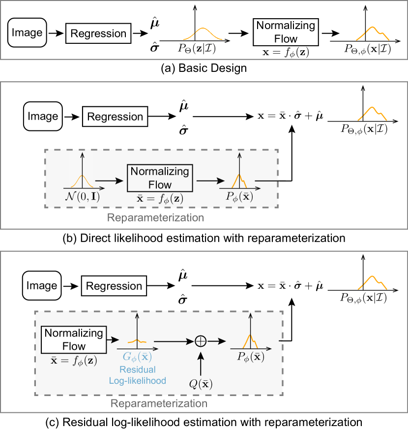
Figure 2: Illustrasion of the proposed regression frameworks. (a) The basic design. (b) Direct likelihood estimation with reparameterization. (c) Residual log-likelihood estimation with reparameterization.

Reparameterization.

Although the basic design seems reasonable, it is not feasible in practice. The learning of $f_{\phi}$ relies on the terms $\log\left|\det\frac{\partial f_{\phi}^{-1}}{\partial\boldsymbol{\mu}_{g}}\right|$ and $f^{-1}_{\phi}(\boldsymbol{\mu}_{g})$ in the loss function (Eq. 4). Therefore, $\phi$ will learn to fit the distribution of $\boldsymbol{\mu}_{g}$ across all images. Nevertheless, the distribution that we want to learn is about how the output deviates from the ground truth conditioning on the input image, not the distribution of the ground truth itself across all images.

Here, to make our regression framework feasible and compatible with the off-the-shelf flow models, we further design the regression paradigm with the reparameterization strategy. The new paradigm is illustrated in Fig. 2(b). We assume all the underlying distribution share the same density function family but with different mean and variance conditioning on the input $\mathcal{I}$. Firstly, the flow model $f_{\phi}$ is leveraged to map a zero-mean initial distribution $\bar{\textbf{z}}\sim\mathcal{N}(0,\mathbf{I})$ to a zero-mean deformed distribution $\bar{\textbf{x}}\sim P_{\phi}(\bar{\textbf{x}})$. Then the regression model $\Theta$ predicts two values, $\hat{\boldsymbol{\mu}}$ and $\hat{\boldsymbol{\sigma}}$, to control the position and scale of the distribution. The final distribution $P_{\Theta,\phi}(\mathbf{x}|\mathcal{I})$ is obtained by shifting and rescaling $\bar{\mathbf{x}}$ to $\mathbf{x}$, where $\mathbf{x}=\bar{\mathbf{x}}\cdot\hat{\boldsymbol{\sigma}}+\hat{\boldsymbol{\mu}}$.

Therefore, the loss function with reparameterization can be written as:

$$\mathcal{L}_{\textit{mle}} =-\log P_{\Theta,\phi}(\mathbf{x}|\mathcal{I})\Big{|}_{\mathbf{x}=\boldsymbol{\mu}_{g}}$$ (5)

$$=-\log P_{\phi}(\bar{\boldsymbol{\mu}}_{g})-\log\left|\det\frac{\partial\bar{\boldsymbol{\mu}}_{g}}{\partial{\boldsymbol{\mu}_{g}}}\right|$$

$$=-\log P_{\phi}(\bar{\boldsymbol{\mu}}_{g})+\log\hat{\boldsymbol{\sigma}},$$

where $\bar{\boldsymbol{\mu}}_{g}=(\boldsymbol{\mu}_{g}-\hat{\boldsymbol{\mu}})/\hat{\boldsymbol{\sigma}}$, and ${\partial\bar{\boldsymbol{\mu}}_{g}}/{\partial{\boldsymbol{\mu}_{g}}}=1/\hat{\boldsymbol{\sigma}}$. With the reparameterization design, now the flow model can focus on learning the distribution of $\bar{\boldsymbol{\mu}}_{g}$, which reflects the deviation of the output from the ground truth.

Residual Log-likelihood Estimation.

After reparameterization, the regression framework can be trained in an end-to-end manner. The training of the regressed value $\hat{\boldsymbol{\mu}}$ and the flow model $f_{\phi}$ are coupled together, depending on the term $\log P_{\phi}(\bar{\boldsymbol{\mu}}_{g})$ in the loss function (Eq. 5). However, there are intricate dependencies between these two models. The training of the regression model entirely relies on the distribution estimated by the flow model $f_{\phi}$. At the beginning stage of training, the shape of the distribution is far from correct, which increases the difficulty to train the regression model and might degrade the model performance.

To facilitate the training process, we develop a gradient shortcut to reduce the dependence between these two models. Formally, the distribution estimated by the flow model $P_{\phi}(\bar{\mathbf{x}})$ is trying to fit the optimal underlying distribution $P_{\textit{opt}}(\bar{\mathbf{x}})$, which can be split into three terms:

$$\log P_{\textit{opt}}(\bar{\mathbf{x}}) =\log\left(Q(\bar{\mathbf{x}})\cdot\frac{P_{\textit{opt}}(\bar{\mathbf{x}})}{s\cdot Q(\bar{\mathbf{x}})}\cdot s\right)$$ (6)

$$=\log Q(\bar{\mathbf{x}})+\log\frac{P_{\textit{opt}}(\bar{\mathbf{x}})}{s\cdot Q(\bar{\mathbf{x}})}+\log s,$$

where the term $Q(\bar{\mathbf{x}})$ can be a simple distribution, e.g. Gaussian distribution $Q(\bar{\mathbf{x}})=\mathcal{N}(0,\mathbf{I})$, the term $\log\frac{P_{\textit{opt}}(\bar{\mathbf{x}})}{s\cdot Q(\bar{\mathbf{x}})}$ is what we call residual log-likelihood, and the constant $s$ is to make sure the residual term is a distribution. We assume that $Q(\bar{\mathbf{x}})$ can roughly match the underlying distribution but not perfectly. The residual log-likelihood is to compensate for the difference. Thus, we split the log-probability of $P_{\phi}(\bar{\mathbf{x}})$ the same way as Eq. 6:

$$\log P_{\phi}(\bar{\mathbf{x}})=\log Q(\bar{\mathbf{x}})+\log G_{\phi}(\bar{\mathbf{x}})+\log s,$$ (7)

where $G_{\phi}(\bar{\mathbf{x}})$ is the distribution learned by the flow model. The value of $s={\frac{1}{\int G_{\phi}(\bar{\mathbf{x}})Q(\bar{\mathbf{x}})d\bar{\mathbf{x}}}}$ can be approximated by the Riemann sum. The derivation of $s$ is provided in the supplemental document.

In this way, $G_{\phi}(\bar{\mathbf{x}})$ will try to fit the underlying residual likelihood $\frac{P_{\textit{opt}}(\bar{\mathbf{x}})}{s\cdot Q(\bar{\mathbf{x}})}$ instead of learning the entire distribution. Finally, combining the reparameterization design (Eq. 5) and residual log-likelihood estimation (Eq. 7), the total loss function can be defined as:

$$\mathcal{L}_{\textit{rle}} =-\log P_{\Theta,\phi}(\mathbf{x}|\mathcal{I})\Big{|}_{\mathbf{x}=\boldsymbol{\mu}_{g}}$$ (8)

$$=-\log P_{\phi}(\bar{\boldsymbol{\mu}}_{g})+\log\hat{\boldsymbol{\sigma}}$$

$$=-\log Q(\bar{\boldsymbol{\mu}}_{g})-\log G_{\phi}(\bar{\boldsymbol{\mu}}_{g})-\log s+\log\hat{\boldsymbol{\sigma}}.$$

This process is illustrated in Fig. 2(c).

During training, the backward propagated gradients from $Q(\bar{\boldsymbol{\mu}}_{g})$ do not depend on the flow model, which accelerates the training of the regression model. Besides, as the hypothesis of ResNet [16], it is easier to optimize the residual mapping than to optimize the original unreferenced mapping. To the extreme, if the preset approximation $Q(\bar{\mathbf{x}})$ is optimal, it would be easier to push the residual log-probability to zero than to fit an identity mapping by a stack of invertible mappings in $f_{\phi}$. The effectiveness of the residual log-likelihood estimation is validated in §4.1.

3.3 Implementation Details

In the training phase, the regression model and the flow model are simultaneously optimized in an end-to-end manner. We replace the standard regression loss ($\ell_{1}$ and $\ell_{2}$) with the proposed residual log-likelihood estimation loss $\mathcal{L}_{\textit{rle}}$. The initial density is set to Laplace distribution by default. In the testing phase, the predicted mean $\hat{\boldsymbol{\mu}}$ serves as the regressed output. Therefore, the flow model does not need to be run during inference. This characteristic makes the proposed method flexible and easy to apply to various regression algorithms without any test-time overhead. Besides, the prediction confidence can be obtained from $\hat{\boldsymbol{\sigma}}$:

$$\hat{c}=1-\frac{1}{K}\sum_{i}^{K}\hat{\boldsymbol{\sigma}}_{i},$$ (9)

where $\hat{\boldsymbol{\sigma}}_{i}$ is the learned deviation of the $i$th joint, and $K$ denotes the total number of joints. The deviation $\hat{\boldsymbol{\sigma}}_{i}$ is predicted with a sigmoid function. Hence we have $\hat{\boldsymbol{\sigma}}_{i}\in(0,1)$ and $\hat{c}\in(0,1)$.

Flow Model.

The proposed regression paradigm is agnostic to the flow models. Hence, various off-the-shelf flow models [52, 11, 26, 46, 25] can be applied. In the experiments, we adopt RealNVP [11] for fast training. We denote the invertible function with $L_{\textit{fc}}$ fully-connected layers with $N_{n}$ neurons as $L_{\textit{fc}}\times N_{n}$. We set $L_{\textit{fc}}=3$ and $N_{n}=64$ by default. The flow model is light-weighted and barely affects the training speed. More detailed descriptions of the flow model architecture are provided in the supplemental document (§A).

Tasks.

The proposed regression paradigm is general and is ready for various human pose estimation tasks. In the experiments, we validate the proposed regression paradigm on seven different algorithms in five tasks: single-person 2D pose estimation, top-down 2D pose estimation, one-stage 2D pose estimation, single-stage 3D pose estimation and two-stage 3D pose estimation. Detailed training settings are provided in §4 and §5. The experiments on single-person 2D pose estimation are provided in the supplemental document.

4 Experiments on COCO

We first evaluate the proposed regression paradigm on a large-scale in-the-wild 2D human pose benchmark COCO Keypoint [32].

Implementation Details.

We embed RLE into the top-down approaches and a one-stage approach. For the top-down approach, we adopt a simple architecture consisting of a ResNet-50 [16] backbone, followed by an average pooling layer and an FC layer. The FC layer consists of $K\times 4$ neurons, where $4$ is for $\hat{\boldsymbol{\mu}}$ and $\hat{\boldsymbol{\sigma}}$, and $K=17$ denotes the number of body keypoints. For human detection, we use the person detectors provided by SimplePose [67] for both the validation set and the test-dev set. Data augmentations and training settings follow previous work [55]. The end-to-end approach, Mask R-CNN [15], is also adopted for ablation study. Implementation is based on Detectron2 [12]. The keypoint head is a stack of $8$ convolutional layers, followed by an average pooling layer and an FC layer. We train for $270,000$ iterations, with 4 images per GPU and 4 GPUs in total. Other parameters are the same as the original Detectron2.

For the one-stage approach, we adopt the state-of-the-art method [64]. We replace its 2K-channel regression head with a 4K-channel head for the prediction of both $\hat{\boldsymbol{\mu}}$ and $\hat{\boldsymbol{\sigma}}$. Implementation is based on the official code of [64]. The other training details are the same as them.

Method	# Params	GFLOPs	AP	AP50	AP75
Direct Regression (with $\ell_{1}$)	23.6M	4.0	58.1	82.7	65.0
Regression with DLE	23.6M	4.0	62.7	86.1	70.4
Regression with RLE	23.6M	4.0	70.5	88.5	77.4
Regression with RLE	23.6M	4.0	71.3	88.9	78.3

Table 1: Comparison with the conventional regression paradigm. RLE provides significant improvements with the same test-time computational complexity.

	Method	AP	AP50	AP75
(a)	SimplePose [67]	71.0	89.3	79.0
	Integral Pose [57]	63.0	85.6	70.0
	*Regression with RLE	71.3	88.9	78.3
(b)	HRNet-W32 [55]	74.1	90.0	81.5
	HRNet-W32 + RLE (Regression)	74.3	89.7	80.8
(c)	Mask R-CNN [15]	66.0	86.9	71.5
	Mask R-CNN + RLE	66.7	86.7	72.6
(d)	PointSet Anchor [64]	67.0	87.3	73.5
	PointSet Anchor + RLE	67.4	87.5	73.9

Table 2: Comparison with heatmap-based methods on COCO validation set. The proposed paradigm achieves competitive performance to the heatmap-based methods.

4.1 Main Results

Comparison with Conventional Regression.

To study the effectiveness of the proposed regression paradigm, we compare it with the conventional direct regression method. The direct regression model has the same “ResNet-50 + FC” architecture, and $\ell_{1}$ loss is adopted. The experimental results on COCO validation set are shown in Tab. 1. As shown, the proposed method brings significant improvement (12.4 mAP) to the regression-based method. Then we compare the result with direct likelihood estimation (DLE) to study the effectiveness of residual log-likelihood estimation. The DLE model only adopts the reparameterization strategy and no residual log-likelihood estimation. It is seen that the residual manner provides 7.8 mAP improvements. Like previous work [57], we further adopt the network backbone that pre-trained by the heatmap loss. This model achieves the best performance with 71.3 mAP, which is denoted with $*$.

Note that the flow model does not participate in the inference phase. Therefore, no extra computation is introduced in testing. Besides, the training overhead of the flow model is negligible. Detailed results are reported in the supplemental document (§B). These experiments demonstrate the superiority of the proposed regression paradigm.

Method	Backbone	AP	AP50	AP75	APM	APL
Heatmap-based
CMU-Pose [4]	3CM-3PAF	61.8	84.9	67.5	57.1	68.2
Mask R-CNN [15]	ResNet-50	63.1	87.3	68.7	57.8	71.4
G-RMI [48]	ResNet-101	64.9	85.5	71.3	62.3	70.0
RMPE [13]	PyraNet	72.3	89.2	79.1	68.0	78.6
AE [41]	Hourglass-4	65.5	86.8	72.3	60.6	72.6
PersonLab [47]	ResNet-152	68.7	89.0	75.4	64.1	75.5
CPN [6]	ResNet-Inception	72.1	91.4	80.0	68.7	77.2
SimplePose [67]	ResNet-152	73.7	91.9	81.1	70.3	80.0
Integral [57]	ResNet-101	67.8	88.2	74.8	63.9	74.0
HRNet [55]	HRNet-W48	75.5	92.5	83.3	71.9	81.5
EvoPose [37]	EvoPose2D-L	75.7	91.9	83.1	72.2	81.5
Regression-based
CenterNet [73]	Hourglass-2	63.0	86.8	69.6	58.9	70.4
SPM [45]	Hourglass-8	66.9	88.5	72.9	62.6	73.1
PointSet Anchor [64]	HRNet-W48	68.7	89.9	76.3	64.8	75.3
ResNet + RLE (Ours)	ResNet-152	74.2	91.5	81.9	71.2	79.3
*ResNet + RLE (Ours)	ResNet-152	75.1	91.8	82.8	72.0	80.2
HRNet + RLE (Ours)	HRNet-W48	75.7	92.3	82.9	72.3	81.3

Table 3: Comparison with the SOTA on COCO test-dev.

Comparison with Heatmap-based Methods.

We further compare our regression method with heatmap-based methods. As shown in Tab. 2(a), our regression method outperforms Integral Pose [57] by 7.5 mAP, and the heatmap supervised SimplePose [67] by 0.3 mAP. For the first time, the direct regression method achieves superior performance to the heatmap-based method.

In Tab. 2(b), we also implement RLE with HRNet [55] to show our approach is flexible and can be easily embedded into various backbone networks. Since HRNet maintains high resolution throughout the whole process, we adopt soft-argmax to produce coordinates $\hat{\boldsymbol{\mu}}$ and an FC layer to produce $\hat{\boldsymbol{\sigma}}$. It shows that integral with RLE surpasses conventional heatmap by 0.2 mAP.

Tab. 2(c) shows the superiority of RLE on Mask R-CNN, the end-to-end top-down approach. Our regression version outperforms the heatmap-based Mask R-CNN by 0.7 mAP. In Tab. 2(d), RLE brings 0.4 mAP improvement to the state-of-the-art one-stage approach. Note that the output of PointSet Anchor [64] relies on the heatmap predictions. The regressed values are used for joint association. The superiority of RLE is demonstrated by embedding it in various approaches.

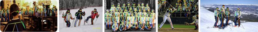
Figure 3: Qualitative results on COCO dataset: containing crowded scenes, occlusions and appearance change.

Comparison with the SOTA on COCO test-dev

In this experiment, we compare the proposed RLE with the state-of-the-art methods on COCO test-dev. Quantitative results are reported in Tab. 3. The proposed regression paradigm significantly outperforms other regression-based methods by 7.0 mAP and achieves state-of-the-art performance. Compared to the same backbone heatmap-based methods, our regression method is 1.4 mAP higher with ResNet-152 and 0.2 mAP higher with HRNet-W48. We demonstrate that heatmap is not the only solution to human pose estimation. Regression-based methods have great potential and can achieve superior performance than heatmap-based methods. Qualitative results are shown in Fig. 3.

Method	Correlation
SimplePose (Heatmap)	0.479
Regression with Gaussian	0.476
Regression with Laplace	0.522
RLE ($Q(\bar{\mathbf{x}})\sim$ Gaussian)	0.540
RLE ($Q(\bar{\mathbf{x}})\sim$ Laplace)	0.553

Table 4: Correlation testing on different methods.

Method	#Params	GFLOPs	GFLOPs of Net. Head	AP
Heatmap-based
Integral Pose [57]	34.0M	9.7	5.7	63.4
SimplePose [67]	34.0M	9.7	5.7	71.0
Regression-based
Regression with RLE	23.6M	4.0	0.0002	71.3

Table 5: Computation complexity and model parameters.

$L_{\textit{fc}}\times N_{n}$	AP	AP50	AP75
$3\times 64$	70.5	88.5	77.4
$3\times 128$	70.2	88.5	77.3
$3\times 256$	69.6	87.9	76.5
$5\times 32$	70.0	88.2	76.8
$5\times 64$	70.3	88.7	77.4

Table 6: Different RealNVP Architecture.

Distribution	AP	AP50	AP75
Const. Variance Gaussian ($\ell_{2}$)	36.6	70.9	33.6
Const. Variance Laplace ($\ell_{1}$)	58.1	82.7	65.0
Gaussian	60.2	82.9	66.6
Laplace	67.4	86.8	74.2
RLE ($Q(\bar{\mathbf{x}})\sim$ Gaussian)	70.0	88.1	76.7
RLE ($Q(\bar{\mathbf{x}})\sim$ Laplace)	70.5	88.5	77.4

Table 7: Initial Density: Performance with different hypotheses of the output distribution.

Correlation with Prediction Correctness.

The estimated standard deviation $\hat{\boldsymbol{\sigma}}$ establishes the correlation with the prediction correctness. The model will output a larger $\hat{\boldsymbol{\sigma}}$ for a more uncertain result. Therefore, $\hat{\boldsymbol{\sigma}}$ plays the same role as the confidence score in the heatmap. We transform the deviation to confidence with Eq. 9. To analysis the correlation of $\hat{\boldsymbol{\sigma}}$ and the prediction correctness, we calculate the Pearson correlation coefficient between the confidence and the OKS to the ground truth on the COCO validation set. The confidence of the heatmap-based prediction [67] is the maximum value of the heatmap. Tab. 6 reveals that RLE has much a stronger correlation to OKS than the heatmap-based method (relative 15.2% improvement). In real-world applications and other downstream tasks, a reliable confidence score is useful and necessary. RLE address the lack of confidence scores in regression-based methods and provide a more reliable score than the heatmap-based methods.

Computation Complexity.

The experimental results of computation complexity and model parameters are listed in Tab. 6. The proposed method achieves comparable results to the heatmap-based methods with significantly lower computation complexity and fewer model parameters. Specifically, the total FLOPs are reduced by 58.8%, and the parameters are reduced by 30.6%. We further calculate the FLOPs of the network head to remove the influence of the network backbone. It shows that the FLOPs of the regression head is only 1/28500 of the heatmap head, which is almost negligible. The computational superiority of our proposed regression paradigm is of great value in the industry.

4.2 Ablation Study

RealNVP Architecture.

In Tab. 11, we compare different network architectures of the RealNVP [11] model. It shows that the final AP keeps stable with different RealNVP architectures. We argue that learning the residual log-likelihood is easy for the flow model. Thus the results are robust to the change of the architecture.

Initial Density.

To examine how the assumption of the output distribution affects the regression performance in the context of MLE, we compare the results of different density functions with our method. The Laplace distribution and Gaussian distribution will degenerate to standard $\ell_{1}$ and $\ell_{2}$ loss if they are assumed to have constant variances. As shown in Tab. 7, the learned distributions of our method provide more than 21.3% improvements. Besides, we study the baselines that assuming the output follows the Gaussian and Laplace distributions with the learnable deviation $\sigma$. The distributions with learnable $\sigma$ outperform those with constant variance, but are still inferior to RLE.

Moreover, different initial densities $Q(\bar{\mathbf{x}})$ for RLE are also tested. There is a large gap between the original Gaussian and Laplace distribution. However, with RLE to learn the change of the density, the difference between these two distributions is significantly reduced. It demonstrates that RLE is robust to different assumptions of the initial density.

5 Experiments on Human3.6M

Human3.6M [21] is an indoor benchmark for 3D pose estimation. For evaluation, MPJPE and PA-MPJPE are used. Following typical protocols [57, 39], we use (S1, S5, S6, S7, S8) for training and (S9, S11) for evaluation.

Implementation Details.

For the single-stage approach, we adopt the same ResNet-50 + FC architecture. The input image is resized to $256\times 256$. Data augmentation includes random scale ($\pm 30\%$), rotation ($\pm 30^{\circ}$), color ($\pm 20\%$) and flip. The learning rate is set to $1\times 10^{-3}$ at first and reduced by a factor of $10$ at the $90$th and $120$ epoch. We use the Adam solver and train for $140$ epochs, with a mini-batch size of $32$ per GPU and $8$ GPUs in total. The 2D and 3D mixed data training strategy (MPII + Human3.6M) is applied. The testing procedure is the same as the previous works [57].

For the two-stage approach, we embed the proposed regression paradigm into the classic baseline [36] and the state-of-the-art model [70]. 2D ground-truth poses are taken as inputs. For data normalization, we follow previous works [70, 50, 71]. The initial learning rate is $1\times 10^{-3}$ and decays $5\%$ after each epoch. We use the Adam solver and train for $80$ epochs, with a mini-batch size of $1024$.

Ablation Study.

In Tab. 8, we report the performance comparison between RLE and the baselines on both single-stage and two-stage approaches. It is seen that RLE reduces the error of single-stage regression baseline by 1.5 mm and the heatmap-based Integral Pose [57] by 0.6 mm. Besides, without 3D heatmaps, our regression method significantly reduces the FLOPs by 61.7% and the model parameters by 30.6%. For the two-stage approach, RLE brings 2.7 mm improvement to the regression baseline without any test-time overhead.

Method	#Params	GFLOPs	MPJPE $\downarrow$	PA-MPJPE $\downarrow$
Single-stage
Direct Regression	23.8M	5.4	50.1	39.3
Integral Pose [57]	34.3M	14.1	49.2	39.1
Regression with RLE	23.8M	5.4	48.6	38.5
Two-stage
FC Baseline	4.3M	0.275	43.6	33.2
FC Baseline + RLE	4.3M	0.275	40.9	31.1

Table 8: Ablation study on Human3.6M.

Method	Sun [56]	Nibali [44]	Sun [57]	Moon [39]	Zhou [72]	Ours
#Params	-	57.9M	34.3M	34.3M	49.6M	23.8M
GFLOPs	-	29.3	14.1	14.1	41.4	5.4
MPJPE	59.1	49.5	49.6	53.3	47.7	48.6

Table 9: Single-stage Results on Human3.6M.

Method	Choi [10]	Martinez [36]	Zhao [71]	Fang [14]	Liu [33]	Zeng [70]	Ours
MPJPE	55.5	45.5	43.8	42.5	37.8	36.5	36.3

Table 10: Two-stage Results on Human3.6M. Our result is based on SRNet [70] with RLE.

Comparison with the State-of-the-art.

In this experiment, we compare the proposed regression paradigm with both single-stage and two-stage state-of-the-art methods in Tab. 9 and Tab. 10. For single-stage, our method achieves comparable performance to the state-of-the-art methods while reducing the FLOPs by 86.7%. The model parameters and FLOPs are calculated using the official code of these methods. Note that [72] only releases the testing code. For fare comparison, we re-train the model with the same training settings as ours. For two-stage, our method is based on SRNet [70] with RLE. It achieves state-of-the-art performance by 0.2 mm improvement to the original SRNet.

6 Conclusion

In this paper, we propose a novel and effective regression paradigm from the perspective of maximum likelihood estimation. The learning process is to maximize the probability of the observation. We leverage the normalizing flow model to learn the residual log-likelihood w.r.t. to the tractable initial density function. Comprehensive experiments are conducted to validate the efficacy of the proposed paradigm. For the first time, the regression-based methods achieve superior performance to the heatmap-based methods. Regression-based methods are efficient and flexible. We hope our method would inspire the field to rethink the potential of regression.

Appendix

In the supplemental document, we provide:

• A more detailed explanation of normalizing flows and RealNVP [11].

• Experiments on MPII dataset.

• Additional ablation experiments.

• Visualization of the learn distribution.

• The derivation of $s$ in RLE.

• Pseudocode for the proposed method.

• Qualitative results on COCO, MPII and Human3.6M datasets.

• Extended experiments on retina OCT segmantation dataset.

Appendix A Normalizing Flows

The idea of normalizing flows is to represent a complex distribution $P_{\phi}(\bar{\mathbf{x}})$ by transforming a much simpler distribution $P({\bar{\mathbf{z}}})$ with a learnable function $\bar{\mathbf{x}}=f_{\phi}(\bar{\mathbf{z}})$. As described in §3.2, the probability of $P_{\phi}(\mathbf{x})$ is calculated as:

$$\log P_{\phi}(\bar{\mathbf{x}})=\log P({\bar{\mathbf{z}}})+\log\left|\det\frac{\partial f_{\phi}^{-1}}{\partial\bar{\mathbf{x}}}\right|.$$ (10)

The function $f_{\phi}$ must be invertible since we need to calculate $\bar{\mathbf{z}}=f_{\phi}^{-1}(\bar{\mathbf{x}})$. In practice, we can compose several simple mappings successively to construct arbitrarily complex functions, i.e. $\mathbf{x}=f_{\phi}(\mathbf{z})=f_{K}\circ\cdots\circ f_{2}\circ f_{1}(\mathbf{z})$, where $K$ denotes the number of mapping functions and $\mathbf{z}_{K}=\mathbf{x}$. The log-probability of $\mathbf{x}$ becomes:

$$\log P_{\Theta}(\mathbf{x}|\mathcal{I})=\log P_{\Theta}(\mathbf{z}|\mathcal{I})+\sum_{k=1}^{K}\log\left|\det\frac{\partial f_{k}^{-1}}{\partial\mathbf{z}_{k}}\right|.$$ (11)

RealNVP.

In our paper, we adopt RealNVP [11] to learn the underlying residual log-likelihood. RealNVP design each layer $f_{k}$ as:

$$f_{k}(\bar{\mathbf{z}}_{{k-1},0:d},\bar{\mathbf{z}}_{{k-1},d:D})$$ (12)

$$= (\bar{\mathbf{z}}_{{k-1},0:d},\bar{\mathbf{z}}_{{k-1},d:D}\odot e^{g_{k}(\bar{\mathbf{z}}_{{k-1},0:d}}+h_{k}(\bar{\mathbf{z}}_{{k-1},0:d})),$$

where $g_{k},h_{k}:\mathbb{R}^{d}\rightarrow\mathbb{R}^{D-d}$ are two arbitrary neural networks, $D$ is the dimension of the input vectors, and $d$ is the splitting location of the $D$-dimensional variable. The $\odot$ operator represents the pointwise product. In order to chain multiple functions $f_{k}$, the input is permuted before each step. $K$ is set to $6$ in our experiments. In each function $f_{k}$, we adopt $L_{\textit{fc}}$ fully-connected layers with $N_{n}$ neurons for both $g_{k}$ and $h_{k}$. Each fully-connected layer is followed by a Leaky-RELU [35] layer.

	FLOPs	#Params	AP	AP50	AP75
$3\times 64$	1.8M	53.8K	70.5	88.5	77.4
$3\times 128$	6.9M	205.8K	70.2	88.5	77.3
$3\times 256$	27.3M	804.8K	69.6	87.9	76.5
$5\times 32$	1.3M	40.0K	70.0	88.2	76.8
$5\times 64$	5.2M	153.6K	70.3	88.7	77.4

Table 11: Computation complexity and parameters of RealNVP during training.

Computation Complexity.

The RealNVP model is fast and light-weighted. The computation complexity and model parameters during training are listed in Tab. 11. It is seen that the flow models are computational and storage efficient. The overhead during training is negligible.

Appendix B Experiments on MPII

In multi-person pose estimation, the final mAP is affected by both the location accuracy and the confidence score. To study how RLE affect the location accuracy and eliminate the impact of the confidence score, we evaluate the proposed regression paradigm on MPII [1] dataset. Following previous settings [57], PCK and AUC are used for evaluation. We adopt the same ResNet-50 + FC model for single-person 2D pose estimation. Data augmentations and training settings are similar to the experiments on COCO.

Method	PCKh@0.5	PCKh@0.1	AUC
Direct Regression	83.8	23.6	52.6
SimplePose (Heatmap) [67]	87.1	25.4	56.2
Regression with RLE	85.5	26.7	55.1
Regression with RLE	85.8	27.1	55.5

Table 12: Effect of Residual Log-likelihood Estimation on MPII validation set.

Ablation Study.

Tab. 12 shows the comparison among methods using heatmaps, direct regression and RLE. RLE surpasses the direct regression baseline. While MPII is less challenging than COCO, the improvement is still significant on PCKh@0.1 (relative 13.1%) with high localization accuracy requirement. Compared to the heatmap-based method, RLE achieves comparable performance (5.1% PCKh@0.1 higher, 1.8% PCKh@0.5 lower and 1.9% AUC lower), and the pre-trained model achieves the best PCKh@0.1 results. RLE shows the superiority in high precision localization.

Appendix C Ablation Study

Method	MPII			Human3.6M
	PCKh@0.5	PCKh@0.1	AUC	MPJPE	PA-MPJPE
DLE	84.3	25.3	53.5	51.0	39.8
RLE	85.5	26.7	55.1	48.6	38.5

Table 13: Comparison between DLE and RLE on MPII and Human3.6M.

Comparison between DLE and RLE.

In this work, direct likelihood estimation (DLE) refers to the model that only adopts the reparameterization strategy to estimate the likelihood function. The comparison is conducted on COCO [32] validation set in the paper. Here, we provide more comparison results on MPII [1] and Human3.6M [21] datasets (Tab. 13). It is seen that RLE shows consistent improvements over DLE.

Method	reg. loss weight	hm. loss weight	AP
Direct Regression ($\ell_{1}$)	1	1	57.5
Direct Regression ($\ell_{1}$)	1	0.5	56.7
Direct Regression ($\ell_{1}$)	1	0	58.1
RLE	1	1	70.4
RLE	1	0.5	70.2
RLE	1	0	70.5

Table 14: Effect of the auxiliary heatmap loss.

Auxiliary Heatmap Loss.

In this experiment, we add an auxiliary heatmap loss to the regression model and study its effect. The regression models follow the top-down framework with the “ResNet-50 + FC” architecture. To train the model with the auxiliary loss, the ResNet-50 backbone is followed by 3 deconv layers as SimplePose [67] to generate heatmaps. The deconv layers are parallel to the FC layer. Thus the model can predict both heatmaps and the regressed coordinates. It shows that multi-task loss barely brings performance improvements.

Robustness to Occlusion.

The regression-based methods predict the body joints in a holistic manner, meaning that they would predict all joints even in cases of occlusions and truncations. In this experiment, we study the impact of occlusion on RLE compared with the heatmap-based method. Similar to PARE [27], we add gray squares on the areas of various joints and study the impact on other joints. Results of Integral Pose [57] and RLE are reported in Table. 15 and Table. 16, respectively. It is seen that RLE improves the occlusion robustness of all joints.

	Ankle	Knee	Hip	Wrist	Elbow	Shoulder	Head
Ankle	135.79	60.2	22.72	86.71	70.05	52.09	50.16
Knee	91.45	70.56	23.73	94.64	72.31	55.71	53.58
Hip	87.98	64.04	28.78	153.02	107	78.98	77.15
Wrist	80.77	56.05	27.44	216.17	127.28	74.29	77.85
Elbow	80.25	57.46	27.87	212.46	156.66	77.71	68.85
Shoulder	73.3	48.01	24.5	146.64	113.5	97.39	159.67
Head	68.71	44.44	21.62	85.87	69.43	52.25	53.39

Table 15: Per joint occlusion sensitivity analysis of Integral Pose [57].

	Ankle	Knee	Hip	Wrist	Elbow	Shoulder	Head
Ankle	117.86	59.69	19.76	83.93	66.68	51.08	48.83
Knee	94.96	68.27	20.64	92.77	72.96	54.24	50.69
Hip	88.39	57.46	19.98	139.47	100.86	75.25	75.79
Wrist	83.06	53.64	21.3	200.18	125.16	73.51	74.73
Elbow	81.45	55.05	24.38	208.01	154.6	76.82	67.06
Shoulder	95.77	54.76	20.93	152.28	118.28	96.01	162.34
Head	72.27	44.44	18.65	83.34	66.14	49.81	48.73

Table 16: Per joint occlusion sensitivity analysis of RLE.

Robustness to Truncation.

When facing truncations, regression-based methods can infer the joints outside the input image, while heatmap-based methods failed. This characteristic of regression-based methods makes them robust to crowded cases, where human detection methods are prone to fail. Qualitative comparison between the heatmap-based method and RLE on truncations are shown in Fig. 5. Only the contents inside the bounding boxes are fed to the pose estimation models.

Figure 4: Visualization of (a) the learned distribution, (b) Laplace distribution, and (c) Gaussian distribution.

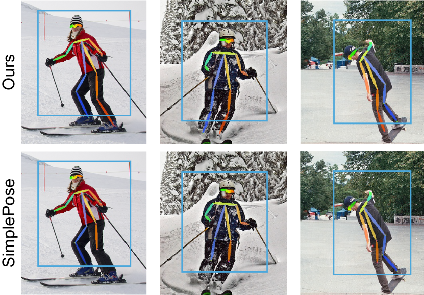
Figure 5: Qualitative comparison on truncations. Top: RLE. Bottom: Heatmap-based SimplePose. Only the contents inside the bounding boxes (blue) are fed to models.

Appendix D Visualization of the Learned Distribution

The visualization of the learned distribution is illustrated in Fig. 4. The learned distribution has a more sharp peak than the Gaussian distribution and a more smooth edge than the Laplace distribution.

Appendix E Derivation of $s$ in RLE

As Eq. 7 in the paper, we have:

$$\log P_{\phi}(\bar{\mathbf{x}})d\bar{\mathbf{x}}=\log Q(\bar{\mathbf{x}})+\log G_{\phi}(\bar{\mathbf{x}})+\log s.$$ (13)

Thus $P_{\phi}(\bar{\mathbf{x}})=Q(\bar{\mathbf{x}})G_{\phi}(\bar{\mathbf{x}})s$. Since $P_{\phi}(\bar{\mathbf{x}})$ should be a distribution, its integral equals to one:

$$\int P_{\phi}(\bar{\mathbf{x}}) =\int Q(\bar{\mathbf{x}})G_{\phi}(\bar{\mathbf{x}})sd\bar{\mathbf{x}}$$ (14)

$$=s\int Q(\bar{\mathbf{x}})G_{\phi}(\bar{\mathbf{x}})d\bar{\mathbf{x}}=1.$$

We obtain:

$$s=\frac{1}{\int Q(\bar{\mathbf{x}})G_{\phi}(\bar{\mathbf{x}})d\bar{\mathbf{x}}}.$$ (15)

The integral is approximate by the Riemann sum. Therefore, within the interval $[a,b]$, the value of $s$ can be calculated as:

$$s\approx\frac{1}{\sum_{i=1}^{N}Q(a+i\Delta\mathbf{x})G_{\phi}(a+i\Delta\mathbf{x})\Delta\mathbf{x}},$$ (16)

where $\Delta\mathbf{x}=\frac{b-a}{N}$ and $N$ is the total number of subintervals. The interval can set to $[-5,5]$ in practice, since the value of $Q(\bar{\mathbf{x}})$ is close to zero outside this interval. To accurately calculate $s$, $N$ should be large enough to obtain a small step $\Delta\mathbf{x}$. In other words, the flow model needs to run $N$ times for calculation, which takes additional computation resources. Interestingly, in our experiments, we find that the term $\log s$ in the loss function is not necessary. As shown in Tab. 17, the effectiveness of RLE over DLE comes from the gradient shortcut in $Q(\bar{\mathbf{x}})$. The term $s$ barely affects the results and can be removed to save computation resources. Therefore, in our implementation, we drop the term $\log s$ for simplicity.

Loss	FLOPs of RealNVP	AP	AP50	AP75
DLE	1.8M	62.7	86.1	70.4
RLE ($Q+G$)	1.8M	70.5	88.5	77.4
RLE ($Q+G+s$)	44.2M	70.5	88.6	77.4

Table 17: Effectiveness of RLE on COCO validation set. FLOPs in the training phase are reported.

Appendix F Pseudocode for the Proposed Method

The pseudocode of the proposed regression paradigm is given in Alg. 1 (training) and Alg. 2 (inference). It is seen in Alg. 2 that the flow model does not participate in the inference phase. Thus the proposed method won’t cause any test-time overhead.

Algorithm 1 Pseudocode for training in a PyTorch-like style.

⬇

# Training

for imgs, gt_mu in train_loader:

# Regression model predicts ‘hat_mu’, ‘hat_sigma’ to control the position and scale

hat_mu, hat_sigma = reg_model(imgs)

# Calculate the deviation ‘bar_mu’

bar_mu = (gt_mu - hat_mu) / hat_sigma

# Estimate the log-probability of ‘bar_mu’ from the flow model

log_phi = flow_model.log_prob(bar_mu)

if use_residual:

# Loss for residual log-likelihood estimation

# Q is the preset density function

loss = - torch.log(Q(bar_mu)) - log_phi + torch.log(hat_sigma)

else:

# Loss for direct log-likelihood estimation

loss = - log_phi + torch.log(hat_sigma)

Algorithm 2 Pseudocode for inference in a PyTorch-like style.

⬇

# Inference

for imgs in test_loader:

# Run the regression model

hat_mu, hat_sigma = reg_model(imgs)

# Calculate the confidence scores

conf = 1 - torch.mean(hat_sigma, dim=1)

output = dict(

coord=hat_mu,

confidence=conf

)

Appendix G Qualitative Results

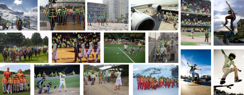
Figure 6: Qualitative results on COCO dataset: containing crowded scenes, occlusions, appearance change and motion blur.

Figure 7: Qualitative results on MPII dataset.

Figure 8: Qualitative results on Human3.6M dataset.

Additional qualitative results on COCO, MPII and Human3.6M datasets are shown in Fig. 6, Fig. 7 and Fig. 8.

Appendix H Experiments on Retina Segmentation

To study the effectiveness and generalization of the proposed regression paradigm, we conduct experiments on boundary regression for retina segmentation from optical coherence tomography (OCT). We evaluate our methods on the publicly available DME dataset [9]. It contains $110$ B-scans from $10$ patients with severe DME pathology.

We follow the model architecture of the previous method [17] and replace the output layer with a fully-connected layer for regression. The learning rate is set to $1\times 10^{-4}$. We use the Adam solver and train for $200$ epochs, with a mini-batch size of $2$. Quantitative results are reported in Tab. 18. It shows that RLE significantly reduces the regression error. We hope our method can be extended to more areas and bring a new perspective to the community.

Method	Mean Error
Direct Regression	18.1
Regression with RLE	3.1

Table 18: Effect of Residual Log-likelihood Estimation on DME dataset.

References

- [1] Mykhaylo Andriluka, Leonid Pishchulin, Peter Gehler, and Bernt Schiele. 2d human pose estimation: New benchmark and state of the art analysis. In CVPR, 2014.
- [2] Jonathan T Barron. A general and adaptive robust loss function. In CVPR, 2019.
- [3] Benjamin Biggs, Sébastien Ehrhadt, Hanbyul Joo, Benjamin Graham, Andrea Vedaldi, and David Novotny. 3d multi-bodies: Fitting sets of plausible 3d human models to ambiguous image data. In NeurIPS, 2020.
- [4] Zhe Cao, Tomas Simon, Shih-En Wei, and Yaser Sheikh. Realtime multi-person 2d pose estimation using part affinity fields. In CVPR, 2017.
- [5] Joao Carreira, Pulkit Agrawal, Katerina Fragkiadaki, and Jitendra Malik. Human pose estimation with iterative error feedback. In CVPR, 2016.
- [6] Yilun Chen, Zhicheng Wang, Yuxiang Peng, Zhiqiang Zhang, Gang Yu, and Jian Sun. Cascaded pyramid network for multi-person pose estimation. In CVPR, 2018.
- [7] Zerui Chen, Yiru Guo, Yan Huang, and Liang Wang. Learning depth-aware heatmaps for 3d human pose estimation in the wild. In BMVC, 2019.
- [8] Bowen Cheng, Bin Xiao, Jingdong Wang, Honghui Shi, Thomas S Huang, and Lei Zhang. Higherhrnet: Scale-aware representation learning for bottom-up human pose estimation. In CVPR, 2020.
- [9] Stephanie J Chiu, Michael J Allingham, Priyatham S Mettu, Scott W Cousins, Joseph A Izatt, and Sina Farsiu. Kernel regression based segmentation of optical coherence tomography images with diabetic macular edema. Biomedical optics express, 2015.
- [10] Hongsuk Choi, Gyeongsik Moon, and Kyoung Mu Lee. Pose2mesh: Graph convolutional network for 3d human pose and mesh recovery from a 2d human pose, 2020.
- [11] Laurent Dinh, Jascha Sohl-Dickstein, and Samy Bengio. Density estimation using real nvp. In ICRL, 2016.
- [12] facebookresearch. Detectron2. https://github.com/facebookresearch/detectron2, 2021.
- [13] Hao-Shu Fang, Shuqin Xie, Yu-Wing Tai, and Cewu Lu. Rmpe: Regional multi-person pose estimation. In ICCV, 2017.
- [14] Hao-Shu Fang, Yuanlu Xu, Wenguan Wang, Xiaobai Liu, and Song-Chun Zhu. Learning pose grammar to encode human body configuration for 3d pose estimation. In AAAI, 2018.
- [15] Kaiming He, Georgia Gkioxari, Piotr Dollár, and Ross Girshick. Mask r-cnn. In ICCV, 2017.
- [16] Kaiming He, Xiangyu Zhang, Shaoqing Ren, and Jian Sun. Deep residual learning for image recognition. In CVPR, 2016.
- [17] Yufan He, Aaron Carass, Yihao Liu, Bruno M Jedynak, Sharon D Solomon, Shiv Saidha, Peter A Calabresi, and Jerry L Prince. Fully convolutional boundary regression for retina oct segmentation. In MICCAI, 2019.
- [18] Yihui He, Chenchen Zhu, Jianren Wang, Marios Savvides, and Xiangyu Zhang. Bounding box regression with uncertainty for accurate object detection. In CVPR, 2019.
- [19] Ehsan Imani and Martha White. Improving regression performance with distributional losses. In ICML, 2018.
- [20] Eldar Insafutdinov, Leonid Pishchulin, Bjoern Andres, Mykhaylo Andriluka, and Bernt Schiele. Deepercut: A deeper, stronger, and faster multi-person pose estimation model. In ECCV, 2016.
- [21] Catalin Ionescu, Dragos Papava, Vlad Olaru, and Cristian Sminchisescu. Human3.6m: Large scale datasets and predictive methods for 3D human sensing in natural environments. TPAMI, 2014.
- [22] Umar Iqbal and Juergen Gall. Multi-person pose estimation with local joint-to-person associations. In ECCV, 2016.
- [23] Sam Johnson and Mark Everingham. Clustered pose and nonlinear appearance models for human pose estimation. In BMVC, 2010.
- [24] Sam Johnson and Mark Everingham. Learning effective human pose estimation from inaccurate annotation. In CVPR, 2011.
- [25] Diederik P Kingma and Prafulla Dhariwal. Glow: Generative flow with invertible 1x1 convolutions. In NeurIPS, 2018.
- [26] Diederik P Kingma, Tim Salimans, Rafal Jozefowicz, Xi Chen, Ilya Sutskever, and Max Welling. Improving variational inference with inverse autoregressive flow, 2016.
- [27] Muhammed Kocabas, Chun-Hao P Huang, Otmar Hilliges, and Michael J Black. Pare: Part attention regressor for 3d human body estimation. arXiv preprint arXiv:2104.08527, 2021.
- [28] Youngwan Lee, Joong-won Hwang, Hyung-Il Kim, Kimin Yun, and Joungyoul Park. Localization uncertainty estimation for anchor-free object detection. arXiv preprint arXiv:2006.15607, 2020.
- [29] Chen Li and Gim Hee Lee. Generating multiple hypotheses for 3d human pose estimation with mixture density network. In CVPR, 2019.
- [30] Jiefeng Li, Can Wang, Hao Zhu, Yihuan Mao, Hao-Shu Fang, and Cewu Lu. Crowdpose: Efficient crowded scenes pose estimation and a new benchmark. In CVPR, 2019.
- [31] Jiefeng Li, Chao Xu, Zhicun Chen, Siyuan Bian, Lixin Yang, and Cewu Lu. Hybrik: A hybrid analytical-neural inverse kinematics solution for 3d human pose and shape estimation. In CVPR, 2021.
- [32] Tsung-Yi Lin, Michael Maire, Serge Belongie, James Hays, Pietro Perona, Deva Ramanan, Piotr Dollár, and C Lawrence Zitnick. Microsoft COCO: Common objects in context. In ECCV, 2014.
- [33] Kenkun Liu, Rongqi Ding, Zhiming Zou, Le Wang, and Wei Tang. A comprehensive study of weight sharing in graph networks for 3d human pose estimation, 2020.
- [34] Diogo C Luvizon, Hedi Tabia, and David Picard. Human pose regression by combining indirect part detection and contextual information. Computers & Graphics, 2019.
- [35] Andrew L Maas, Awni Y Hannun, and Andrew Y Ng. Rectifier nonlinearities improve neural network acoustic models. In ICML, 2013.
- [36] Julieta Martinez, Rayat Hossain, Javier Romero, and James J Little. A simple yet effective baseline for 3d human pose estimation. In ICCV, 2017.
- [37] William McNally, Kanav Vats, Alexander Wong, and John McPhee. Evopose2d: Pushing the boundaries of 2d human pose estimation using neuroevolution. arXiv preprint arXiv:2011.08446, 2020.
- [38] Dushyant Mehta, Helge Rhodin, Dan Casas, Pascal Fua, Oleksandr Sotnychenko, Weipeng Xu, and Christian Theobalt. Monocular 3D human pose estimation in the wild using improved cnn supervision, 2017.
- [39] Gyeongsik Moon, Ju Yong Chang, and Kyoung Mu Lee. Camera distance-aware top-down approach for 3D multi-person pose estimation from a single rgb image. In ICCV, 2019.
- [40] Natalia Neverova, David Novotny, and Andrea Vedaldi. Correlated uncertainty for learning dense correspondences from noisy labels. In NeurIPS, 2019.
- [41] Alejandro Newell, Zhiao Huang, and Jia Deng. Associative embedding: End-to-end learning for joint detection and grouping. In NeurIPS, 2017.
- [42] Alejandro Newell, Kaiyu Yang, and Jia Deng. Stacked hourglass networks for human pose estimation. In ECCV, 2016.
- [43] Aiden Nibali, Zhen He, Stuart Morgan, and Luke Prendergast. Numerical coordinate regression with convolutional neural networks. arXiv preprint arXiv:1801.07372, 2018.
- [44] Aiden Nibali, Zhen He, Stuart Morgan, and Luke Prendergast. 3d human pose estimation with 2d marginal heatmaps. In WACV, 2019.
- [45] Xuecheng Nie, Jiashi Feng, Jianfeng Zhang, and Shuicheng Yan. Single-stage multi-person pose machines. In ICCV, 2019.
- [46] George Papamakarios, Theo Pavlakou, and Iain Murray. Masked autoregressive flow for density estimation, 2017.
- [47] George Papandreou, Tyler Zhu, Liang-Chieh Chen, Spyros Gidaris, Jonathan Tompson, and Kevin Murphy. Personlab: Person pose estimation and instance segmentation with a bottom-up, part-based, geometric embedding model. In ECCV, 2018.
- [48] George Papandreou, Tyler Zhu, Nori Kanazawa, Alexander Toshev, Jonathan Tompson, Chris Bregler, and Kevin Murphy. Towards accurate multi-person pose estimation in the wild. In CVPR, 2017.
- [49] Georgios Pavlakos, Xiaowei Zhou, Konstantinos G Derpanis, and Kostas Daniilidis. Coarse-to-fine volumetric prediction for single-image 3d human pose, 2017.
- [50] Dario Pavllo, Christoph Feichtenhofer, David Grangier, and Michael Auli. 3d human pose estimation in video with temporal convolutions and semi-supervised training. In CVPR, 2019.
- [51] Leonid Pishchulin, Eldar Insafutdinov, Siyu Tang, Bjoern Andres, Mykhaylo Andriluka, Peter V Gehler, and Bernt Schiele. Deepcut: Joint subset partition and labeling for multi person pose estimation. In CVPR, 2016.
- [52] Danilo Rezende and Shakir Mohamed. Variational inference with normalizing flows. In ICML, 2015.
- [53] Gregory Rogez, Philippe Weinzaepfel, and Cordelia Schmid. Lcr-net: Localization-classification-regression for human pose. In CVPR, 2017.
- [54] Gregory Rogez, Philippe Weinzaepfel, and Cordelia Schmid. Lcr-net++: Multi-person 2d and 3d pose detection in natural images. TPAMI, 2019.
- [55] Ke Sun, Bin Xiao, Dong Liu, and Jingdong Wang. Deep high-resolution representation learning for human pose estimation. In CVPR, 2019.
- [56] Xiao Sun, Jiaxiang Shang, Shuang Liang, and Yichen Wei. Compositional human pose regression. In ICCV, 2017.
- [57] Xiao Sun, Bin Xiao, Fangyin Wei, Shuang Liang, and Yichen Wei. Integral human pose regression. In ECCV, 2018.
- [58] Zhi Tian, Hao Chen, and Chunhua Shen. Directpose: Direct end-to-end multi-person pose estimation. arXiv preprint arXiv:1911.07451, 2019.
- [59] Jonathan Tompson, Ross Goroshin, Arjun Jain, Yann LeCun, and Christoph Bregler. Efficient object localization using convolutional networks. In CVPR, 2015.
- [60] Jonathan J Tompson, Arjun Jain, Yann LeCun, and Christoph Bregler. Joint training of a convolutional network and a graphical model for human pose estimation. NeurIPS, 2014.
- [61] Alexander Toshev and Christian Szegedy. Deeppose: Human pose estimation via deep neural networks. In CVPR, 2014.
- [62] Can Wang, Jiefeng Li, Wentao Liu, Chen Qian, and Cewu Lu. Hmor: Hierarchical multi-person ordinal relations for monocular multi-person 3d pose estimation. In ECCV, 2020.
- [63] Luyang Wang, Yan Chen, Zhenhua Guo, Keyuan Qian, Mude Lin, Hongsheng Li, and Jimmy S Ren. Generalizing monocular 3d human pose estimation in the wild, 2019.
- [64] Fangyun Wei, Xiao Sun, Hongyang Li, Jingdong Wang, and Stephen Lin. Point-set anchors for object detection, instance segmentation and pose estimation. In ECCV, 2020.
- [65] Shih-En Wei, Varun Ramakrishna, Takeo Kanade, and Yaser Sheikh. Convolutional pose machines. In CVPR, 2016.
- [66] Lijun Wu, Fei Tian, Yingce Xia, Yang Fan, Tao Qin, Jianhuang Lai, and Tie-Yan Liu. Learning to teach with dynamic loss functions. In NeurIPS, 2018.
- [67] Bin Xiao, Haiping Wu, and Yichen Wei. Simple baselines for human pose estimation and tracking. In ECCV, 2018.
- [68] Hongyi Xu, Eduard Gabriel Bazavan, Andrei Zanfir, William T Freeman, Rahul Sukthankar, and Cristian Sminchisescu. Ghum & ghuml: Generative 3d human shape and articulated pose models. In CVPR, 2020.
- [69] Andrei Zanfir, Eduard Gabriel Bazavan, Hongyi Xu, Bill Freeman, Rahul Sukthankar, and Cristian Sminchisescu. Weakly supervised 3d human pose and shape reconstruction with normalizing flows. ECCV, 2020.
- [70] Ailing Zeng, Xiao Sun, Fuyang Huang, Minhao Liu, Qiang Xu, and Stephen Lin. Srnet: Improving generalization in 3d human pose estimation with a split-and-recombine approach. In ECCV, 2020.
- [71] Long Zhao, Xi Peng, Yu Tian, Mubbasir Kapadia, and Dimitris N. Metaxas. Semantic graph convolutional networks for 3d human pose regression. In CVPR, 2019.
- [72] Kun Zhou, Xiaoguang Han, Nianjuan Jiang, Kui Jia, and Jiangbo Lu. Hemlets pose: Learning part-centric heatmap triplets for accurate 3d human pose estimation. In ICCV, 2019.
- [73] Xingyi Zhou, Dequan Wang, and Philipp Krähenbühl. Objects as points. arXiv preprint arXiv:1904.07850, 2019.