Limiter-based entropy stabilization of semi-discrete and fully discrete schemes for nonlinear hyperbolic problems

Abstract

The algebraic flux correction (AFC) schemes presented in this work constrain a standard continuous finite element discretization of a nonlinear hyperbolic problem to satisfy relevant maximum principles and entropy stability conditions. The desired properties are enforced by applying a limiter to antidiffusive fluxes that represent the difference between the high-order baseline scheme and a property-preserving approximation of Lax–Friedrichs type. In the first step of the limiting procedure, the given target fluxes are adjusted in a way that guarantees preservation of local and/or global bounds. In the second step, additional limiting is performed, if necessary, to ensure the validity of fully discrete and/or semi-discrete entropy inequalities. The limiter-based entropy fixes considered in this work are applicable to finite element discretizations of scalar hyperbolic equations and systems alike. The underlying inequality constraints are formulated using Tadmor’s entropy stability theory.

The proposed limiters impose entropy-conservative or entropy-dissipative bounds on the rate of entropy production by antidiffusive fluxes and Runge–Kutta (RK) time discretizations. Two versions of the fully discrete entropy fix are developed for this purpose. The first one incorporates temporal entropy production into the flux constraints, which makes them more restrictive and dependent on the time step. The second algorithm interprets the final stage of a high-order AFC-RK method as a constrained antidiffusive correction of an implicit low-order scheme (algebraic Lax–Friedrichs in space + backward Euler in time). In this case, iterative flux correction is required, but the inequality constraints are less restrictive and limiting can be performed using algorithms developed for the semi-discrete problem. To motivate the use of limiter-based entropy fixes, we prove a finite element version of the Lax–Wendroff theorem and perform numerical studies for standard test problems. In our numerical experiments, entropy-dissipative schemes converge to correct weak solutions of scalar conservation laws, of the Euler equations, and of the shallow water equations.

tcb@breakable

1 Introduction

It is well known that nonlinear hyperbolic problems may have multiple weak solutions but the one corresponding to the vanishing viscosity limit is unique and satisfies a weak form of an entropy inequality. Moreover, the conserved variables or derived quantities are often known to be bounded in a certain manner. It is therefore essential to use numerical methods that are bound preserving and entropy dissipative. Failure to do so may cause occurrence of nonphysical states or convergence to wrong weak solutions [3, 8, 12, 26, 54].

Many modern high-resolution schemes use limiters to ensure preservation of local bounds or at least positivity preservation for scalar quantities of interest. In the context of finite element approximations, such schemes can be constructed using geometric slope limiting [56] or the framework of algebraic flux correction (AFC) [27] and its extensions to hyperbolic systems [17, 20, 29, 28]. The additional requirement of entropy stability implies that a (semi-)discrete entropy inequality should hold for at least one entropy pair. Entropy-dissipative space discretizations of second and higher order can be designed as in [9, 47, 31] using Tadmor’s criterion [53] of entropy stability for semi-discrete problems. Recent years have witnessed significant advances in the development of high-order entropy-stable schemes that exploit the summation-by-parts (SBP) property of discrete operators collocated at quadrature points [7, 10, 13, 16, 45]. A way to penalize semi-discrete entropy production by solution gradients inside mesh cells was proposed by Abgrall [1] and generalized in [2, 32]. To ensure global entropy stability of a fully discrete scheme, relaxation Runge–Kutta methods were developed by Ketcheson et al. [23, 46]. The fully discrete TECNO-SSP schemes proposed in [55] are globally entropy stable under mild time step restrictions. Methods that ensure the validity of local fully discrete entropy inequalities are still rare. Their development was recently advanced by the work of Kivva [25] and Berthon et al. [5, 6]. The algorithms developed in these publications are closely related to our approach. However, they are currently restricted to explicit finite volume schemes on uniform meshes in 1D.

As of this writing, very few bound-preserving schemes for nonlinear hyperbolic problems are provably entropy stable and vice versa. The AFC scheme proposed in [31] constrains a continuous finite element discretization of a scalar conservation law using a bound-preserving flux limiter and a semi-discrete entropy fix based on Tadmor’s condition. In the present paper, we extend the underlying methodology to arbitrary fluxes, hyperbolic systems, and fully discrete schemes. Instead of constructing entropy-conservative fluxes and adding second-order entropy viscosity, we limit the antidiffusive flux that transforms a property-preserving low-order method into a high-order baseline scheme. We show that the bounds of the inequality constraints for limiter-based entropy fixes can be defined to produce an entropy-conservative or entropy-dissipative scheme. We derive sufficient conditions for the validity of local entropy inequalities and constrain the antidiffusive fluxes accordingly. In addition to a generalized entropy fix for the spatial semi-discretization, we present two algorithms that ensure fully discrete entropy stability. The first one limits entropy production by forward Euler stages of a strong stability preserving Runge–Kutta (RK) method, while the second one constrains the final stage of a general RK method in an iterative manner. We study the effectiveness of each limiter-based entropy fix numerically and prove a Lax–Wendroff-type theorem about convergence of finite element approximations to entropy solutions.

In Section 2 of this paper, we discretize a generic hyperbolic problem (a scalar conservation law or a system) using the continuous Galerkin method and (multi-)linear finite elements. Next, we review the basic principles of algebraic flux correction for space discretizations of this kind. Existing extensions to high-order finite elements and discontinuous Galerkin (DG) methods are cited as well. The new limiter-based entropy fixes are presented in Section 4. The importance of entropy stability for convergence to vanishing viscosity solutions is illustrated by the results of theoretical studies in Section 5 and numerical experiments in Section 6. We close this paper with concluding remarks in Section 7.

2 Continuous FEM for hyperbolic problems

Let $u(\mathbf{x},t)\in\mathbb{R}^{m\times 1}$ denote the local density of $m\in\mathbb{N}$ conserved quantities at the space location $\mathbf{x}\in\mathbb{R}^{d},d\in\{1,2,3\}$ and time $t\geq 0$. Imposing periodic boundary conditions on the boundaries of a spatial domain $\Omega\subset\mathbb{R}^{d}$, we consider the initial value problem

$$\frac{\partial u}{\partial t}+\nabla\cdot\mathbf{f}(u) =0\quad\mbox{in}\ \Omega\times\mathbb{R}^{+},$$ (2.1a)

$$\qquad u(\cdot,0) =u_{0}\quad\mbox{in}\ \Omega,$$ (2.1b)

where $\mathbf{f}(u)=(f_{ki})\in\mathbb{R}^{m\times d}$ is an array of inviscid fluxes and $\nabla\cdot\mathbf{f}=\left(\sum_{i=1}^{d}\frac{\partial f_{ki}}{\partial x_{i}}\right)\in\mathbb{R}^{m\times 1}$. The flux and Jacobian of a projection onto a vector $\mathbf{n}=(n_{i})\in\mathbb{R}^{d\times 1}$ are defined by

$$\mathbf{f}(u)\cdot\mathbf{n}=\left(\sum\limits_{i=1}^{d}f_{ki}n_{i}\right)\in\mathcal{\mathbb{R}}^{m\times 1},\qquad\mathbf{f}^{\prime}(u)\cdot\mathbf{n}=\left(\sum\limits_{i=1}^{d}\frac{\partial f_{ki}}{\partial u_{l}}n_{i}\right)\in\mathbb{R}^{m\times m}.$$

In the multidimensional case ($d>1$), the array $\mathbf{f}^{\prime}(u)=\left(\frac{\partial f_{ki}}{\partial u_{l}}\right)\in\mathbb{R}^{m\times m\times d}$ is composed from Jacobian matrices $\mathbf{f}^{\prime}(u)\cdot\mathbf{e}_{1},\ldots,\mathbf{f}^{\prime}(u)\cdot\mathbf{e}_{d}$, where $\mathbf{e}_{i}$ is the $i$-th unit vector in $\mathbb{R}^{d}$. We assume that (2.1a) is hyperbolic, i.e., that any directional Jacobian $\mathbf{f}^{\prime}(u)\cdot\mathbf{n}$ is diagonalizable with real eigenvalues $\lambda_{1},\ldots,\lambda_{m}$ representing $m$ finite speeds of wave propagation.

Because of hyperbolicity, there exists a convex entropy $\eta:\mathbb{R}^{m}\to\mathbb{R}$ and associated entropy flux $\mathbf{q}:\mathbb{R}^{m}\to\mathbb{R}^{1\times d}$ such that $\mathbf{q}^{\prime}(u)=\eta^{\prime}(u)^{T}\mathbf{f}^{\prime}(u)$ for $\eta^{\prime}(u)=\left(\frac{\partial\eta}{\partial u_{k}}\right)\in\mathbb{R}^{m\times 1}$. If problem (2.1) has a smooth classical solution $u$, the entropy conservation law

$$\frac{\partial\eta(u)}{\partial t}+\nabla\cdot\mathbf{q}(u)=0\qquad\mbox{in}\ \Omega\times\mathbb{R}^{+}$$ (2.2)

can be derived from (2.1a) using multiplication by the vector $v(u)=\eta^{\prime}(u)$ of entropy variables, the chain rule, and the definition of an entropy pair $\{\eta(u),\mathbf{q}(u)\}$. In general, the vanishing viscosity solution of (2.1a) satisfies a weak form of the entropy inequality

$$\frac{\partial\eta(u)}{\partial t}+\nabla\cdot\mathbf{q}(u)\leq 0\qquad\mbox{in}\ \Omega\times\mathbb{R}^{+}$$ (2.3)

for any entropy pair. Hence, entropy is conserved in smooth regions and dissipated at shocks. For the derivation of (2.3) and further details, we refer the reader to Tadmor [53].

When it comes to solving (2.1a) numerically, it is essential to guarantee that a (semi-) discrete version of (2.3) holds for at least one entropy pair. Moreover, a good numerical method should ensure preservation of invariant domains, i.e., produce approximations belonging to a convex set $\mathcal{G}$ if the exact solution of (2.1a) is known to stay in this set [18].

2.1 Consistent Galerkin discretization

We discretize (2.1a) in space using the continuous Galerkin method on a conforming mesh $\mathcal{T}_{h}=\{K^{1},\ldots,K^{E_{h}}\}$ of linear ($\mathbb{P}_{1}$) or multilinear ($\mathbb{Q}_{1}$) finite elements. The numerical solution $u_{h}=\sum_{j=1}^{N_{h}}u_{j}\varphi_{j}$ is expressed in terms of Lagrange basis functions $\varphi_{1},\ldots,\varphi_{N_{h}}$ such that $\sum_{i=1}^{N_{h}}\varphi_{i}\equiv 1$. The basis function $\varphi_{i}$ is associated with a vertex $\mathbf{x}_{i}$ of $\mathcal{T}_{h}$. It has the property that $\varphi_{i}(\mathbf{x}_{j})=\delta_{ij}$. The indices of elements containing $\mathbf{x}_{i}$ are stored in the integer set $\mathcal{E}_{i}$. The global indices of nodes belonging to $K^{e}\in\mathcal{T}_{h}$ are stored in the integer set $\mathcal{N}^{e}$. The computational stencil of node $i$ is defined by the index set $\mathcal{N}_{i}=\bigcup_{e\in\mathcal{E}_{i}}\mathcal{N}^{e}$.

The semi-discrete weak form of (2.1a) with periodic boundary conditions is given by

$$\sum_{e=1}^{E_{h}}\int_{K^{e}}v_{h}\left[\frac{\partial u_{h}}{\partial t}+\nabla\cdot\mathbf{f}(u_{h})\right]\,\mathrm{d}\mathbf{x}=0\qquad\forall v_{h}\in V_{h},$$ (2.4)

where $V_{h}$ is the finite-dimensional space spanned by the basis functions $\varphi_{1},\ldots,\varphi_{N_{h}}$. For any entropy pair $\{\eta(u),\mathbf{q}(u)\}$ and $v(u)=\eta^{\prime}(u)$, the evolution of $\eta(u_{h})$ is governed by [32]

$$\sum_{e=1}^{E_{h}}\int_{K^{e}}\left[\frac{\partial\eta(u_{h})}{\partial t}+\nabla\cdot\mathbf{q}(u_{h})\right]\,\mathrm{d}\mathbf{x}=\sum_{e=1}^{E_{h}}\int_{K^{e}}v(u_{h})\left[\frac{\partial u_{h}}{\partial t}+\nabla\cdot\mathbf{f}(u_{h})\right]\,\mathrm{d}\mathbf{x}.$$ (2.5)

In the scalar case ($m=1$), the right-hand side of (2.5) vanishes due to (2.4) for $v(u_{h})=u_{h}$ corresponding to $\eta(u)=\frac{u^{2}}{2}$. It follows that the continuous Galerkin discretization of (2.1a) satisfies an integral form of (2.2), i.e., is entropy conservative in this particular case [32]. This remarkable property was first discovered by Tadmor [52, 53] in the context of finite volume schemes written as lumped-mass $\mathbb{P}_{1}$ finite element approximations.

Invoking the definition of $u_{h}$ and using the test function $v_{h}=\varphi_{i}$ in (2.4), we obtain

$$\sum_{j\in\mathcal{N}_{i}}m_{ij}\frac{\,\mathrm{d}u_{j}}{\,\mathrm{d}t}+\sum_{e\in\mathcal{E}_{i}}\int_{K^{e}}\varphi_{i}\nabla\cdot\mathbf{f}(u_{h})\,\mathrm{d}\mathbf{x}=0,$$ (2.6)

where

$$m_{ij}=\sum_{e\in\mathcal{E}_{i}\cap\mathcal{E}_{j}}\int_{K^{e}}\varphi_{i}\varphi_{j}\,\mathrm{d}\mathbf{x}$$

is an entry of the consistent mass matrix $M_{C}=(m_{ij})_{i,j=1}^{N_{h}}$. Since $u_{h}$ is differentiable on $K^{e}$, equation (2.4) can be written in the equivalent quasi-linear form

$$\sum_{j\in\mathcal{N}_{i}}\left[m_{ij}\frac{\,\mathrm{d}u_{j}}{\,\mathrm{d}t}+a_{ij}(u_{h})u_{j}\right]=0,$$ (2.7)

where

$$a_{ij}(u_{h})=\sum_{e\in\mathcal{E}_{i}\cap\mathcal{E}_{j}}\int_{K^{e}}\varphi_{i}\mathbf{f}^{\prime}(u_{h})\cdot\nabla\varphi_{j}\,\mathrm{d}\mathbf{x}$$

is an entry of the solution-dependent discrete Jacobian operator $A(u_{h})=(a_{ij}(u_{h}))_{i,j=1}^{N_{h}}$.

2.2 Quadrature-based approximations

The properties of a finite element discretization may change if the integrals are calculated numerically. For example, the use of inexact nodal quadrature transforms the matrix $M_{C}$ into its lumped counterpart $M_{L}=(\delta_{ij}m_{i})_{i,j=1}^{N_{h}}$ with diagonal entries

$$m_{i}=\sum_{e\in\mathcal{E}_{i}}\int_{K^{e}}\varphi_{i}\,\mathrm{d}\mathbf{x}=\sum_{e\in\mathcal{E}_{i}}\int_{K^{e}}\varphi_{i}\underbrace{\left(\sum_{j\in\mathcal{N}_{i}}\varphi_{j}\right)}_{\equiv 1}\,\mathrm{d}\mathbf{x}=\sum_{j\in\mathcal{N}_{i}}m_{ij}.$$

The second-order accurate group finite element approximation [4, 15, 30]

$$\mathbf{f}(u_{h})\approx\mathbf{f}_{h}(u_{h})=\sum_{j=1}^{N_{h}}\mathbf{f}_{j}\,\varphi_{j},\qquad\mathbf{f}_{j}=\mathbf{f}(u_{j})$$ (2.8)

yields a useful inexact quadrature rule for calculating $\int_{K^{e}}\varphi_{i}\nabla\cdot\mathbf{f}(u_{h})\,\mathrm{d}\mathbf{x}$. Replacing $\mathbf{f}(u_{h})$ by $\mathbf{f}_{h}(u_{h})$ in the lumped-mass version of (2.6), we obtain the semi-discrete scheme

$$m_{i}\frac{\,\mathrm{d}u_{i}}{\,\mathrm{d}t}+\sum_{j\in\mathcal{N}_{i}}\mathbf{f}_{j}\cdot\mathbf{c}_{ij}=0,$$ (2.9)

where

$$\mathbf{c}_{ij}=\sum_{e\in\mathcal{E}_{i}\cap\mathcal{E}_{j}}\int_{K^{e}}\varphi_{i}\nabla\varphi_{j}\,\mathrm{d}\mathbf{x}$$

denotes a vector-valued entry of the discrete gradient operator $\mathbf{C}=(\mathbf{c}_{ij})_{i,j=1}^{N_{h}}$. Note that $\sum_{j\in\mathcal{N}_{i}}\mathbf{c}_{ij}=\sum_{j=1}^{N_{h}}\mathbf{c}_{ij}=\mathbf{0}$ since $\sum_{j=1}^{N_{h}}\nabla\varphi_{j}\equiv\nabla 1=\mathbf{0}$ for Lagrange basis functions $\varphi_{j}$. Moreover, $\mathbf{c}_{ji}=-\mathbf{c}_{ij}$ unless $i$ or $j$ is a node on a non-periodic boundary. It follows that

$$\sum_{j\in\mathcal{N}_{i}}\mathbf{f}_{j}\cdot\mathbf{c}_{ij}=\sum_{j\in\mathcal{N}_{i}\backslash\{i\}}(\mathbf{f}_{j}-\mathbf{f}_{i})\cdot\mathbf{c}_{ij}=\sum_{j\in\mathcal{N}_{i}\backslash\{i\}}(\mathbf{f}_{j}+\mathbf{f}_{i})\cdot\mathbf{c}_{ij}=\sum_{j\in\mathcal{N}_{i}}(\mathbf{f}_{j}+\mathbf{f}_{i})\cdot\mathbf{c}_{ij}.$$ (2.10)

As shown in [48, 49], the quadrature-based approximation (2.9) is equivalent to a vertex-centered finite volume method with a centered numerical flux. Many edge-based finite element schemes for compressible flow problems exploit this relationship to finite volumes when it comes to the design of artificial viscosities and flux limiting [27, 40, 41].

Remark 1.

Similarly to DG schemes with inexact quadrature [9], the use of the group finite element formulation (2.8) may cause a lack of entropy stability even in the case $m=1,$ $\eta(u)=\frac{u^{2}}{2}$, in which the consistent Galerkin approximation is entropy stable.

2.3 Algebraic flux correction

The concept of algebraic flux correction (AFC) provides a general framework for converting (2.9) into a property-preserving space discretization of the form [27, 29, 36]

$$m_{i}\frac{\,\mathrm{d}u_{i}}{\,\mathrm{d}t}=\sum_{j\in\mathcal{N}_{i}\backslash\{i\}}[d_{ij}(u_{j}-u_{i})-(\mathbf{f}_{j}-\mathbf{f}_{i})\cdot\mathbf{c}_{ij}+f_{ij}^{*}].$$ (2.11)

The coefficients of the artificial viscosity operator $D=(d_{ij})_{i,j=1}^{N_{h}}$ have the property that

$$\sum_{j\in\mathcal{N}_{i}}d_{ij}=0,\qquad d_{ij}=d_{ji},\qquad i,j=1,\ldots,N_{h}$$

and are chosen in such a way that all relevant inequality constraints (maximum principles, entropy stability conditions etc.) are satisfied in the case $f_{ij}^{*}=0$. We define such artificial viscosity coefficients $d_{ij}$ in Section 3.1. In general, $f_{ij}^{*}=-f_{ji}^{*}$ is supposed to approximate a target flux $f_{ij}=-f_{ji}$ in a property-preserving manner. We discuss the corresponding limiting procedures in Sections 3.2, 3.3, and 4.1–4.3. The discretization to which (2.11) reduces in the case $f_{ij}^{*}=f_{ij}\ \forall j\in\mathcal{N}_{i}\backslash\{i\}$ is typically a stabilized version of (2.6). It may use the group finite element approximation (2.8) and/or high-order stabilization provided that the order of accuracy is preserved. Definitions of (stabilized) target fluxes $f_{ij}$ for $\mathbb{P}_{1}/\mathbb{Q}_{1}$ and higher-order finite element discretizations of (2.1a) can be found in [28, 31, 32]. The fluxes that we constrain in the numerical experiments of this work are defined in Section 6.

3 Invariant domain preserving schemes

3.1 Algebraic Lax–Friedrichs method

As explained above, the definition of the scalar artificial viscosity coefficient $d_{ij}$ for the flux-corrected scheme (2.11) should ensure that its low-order counterpart

$$m_{i}\frac{\,\mathrm{d}u_{i}}{\,\mathrm{d}t}=\sum_{j\in\mathcal{N}_{i}\backslash\{i\}}[d_{ij}(u_{j}-u_{i})-(\mathbf{f}_{j}-\mathbf{f}_{i})\cdot\mathbf{c}_{ij}]$$ (3.1)

is property preserving. An algebraic version of the local Lax–Friedrichs method uses [18, 28]

$$d_{ij}=\begin{cases}\max\{\lambda_{ij}|\mathbf{c}_{ij}|,\lambda_{ji}|\mathbf{c}_{ji}|\}&\mbox{if}\ j\neq i,\\ -\sum_{k\in\mathcal{N}_{i}\backslash\{i\}}d_{ik}&\mbox{if}\ j=i,\end{cases}$$ (3.2)

where $\lambda_{ij}$ is an upper bound for the spectral radius of $A_{ij}(\hat{u})=\mathbf{f}^{\prime}(\hat{u})\cdot\frac{\mathbf{c}_{ij}}{|\mathbf{c}_{ij}|}$ evaluated at an arbitrary convex combination $\hat{u}$ of the states $u_{i}$ and $u_{j}$. As shown by Guermond and Popov [18], this definition of the maximum wave speed $\lambda_{ij}$ guarantees preservation of invariant domains and entropy stability. The first property is a generalized maximum principle. If there is a convex invariant set $\mathcal{G}$ such that $u_{h}(\mathbf{x},0)\in\mathcal{G}$ a.e. in $\Omega$, an invariant domain preserving (IDP) scheme keeps $u_{h}(\mathbf{x},t)$ in $\mathcal{G}$ for all $t>0$. The entropy stability property is needed to avoid convergence to wrong weak solutions. Entropy stable schemes produce approximations that satisfy a (semi-)discrete entropy inequality consistent with (2.3).

Remark 2.

In earlier versions [29, 30, 40] of the algebraic Lax–Friedrichs (ALF) scheme (3.1),(3.2) for nonlinear problems, $\lambda_{ij}$ was taken to be the spectral radius of the Jacobian $A_{ij}(u_{i})$ or of the Roe matrix $\hat{A}_{ij}\in\mathbb{R}^{m\times m}$ such that $\hat{A}_{ij}(u_{j}-u_{i})=(\mathbf{f}_{j}-\mathbf{f}_{i})\cdot\mathbf{c}_{ij}$. Although these definitions work well in practice, the resulting schemes are not provably property-preserving for systems. For linear advection of a scalar conserved quantity with constant velocity, all versions of the ALF method reduce to the discrete upwinding procedure described in [27].

3.2 Bound-preserving convex limiting

To formulate a sufficient condition for an AFC scheme of the form (2.11) to inherit the IDP property of the ALF method (3.1), we consider the equivalent representation

$$m_{i}\frac{\,\mathrm{d}u_{i}}{\,\mathrm{d}t}=\sum_{j\in\mathcal{N}_{i}\backslash\{i\}}2d_{ij}(\bar{u}_{ij}^{*}-u_{i}),\qquad\bar{u}_{ij}^{*}=\bar{u}_{ij}+\frac{f_{ij}^{*}}{2d_{ij}}$$ (3.3)

of (2.11) in terms of the property-preserving intermediate states

$$\bar{u}_{ij}=\frac{u_{j}+u_{i}}{2}-\frac{(\mathbf{f}_{j}-\mathbf{f}_{i})\cdot\mathbf{c}_{ij}}{2d_{ij}}.$$ (3.4)

Let $\mathcal{G}$ be a convex invariant set of the initial value problem (2.1). As noticed by Guermond and Popov [18], the ALF bar state $\bar{u}_{ij}$ represents an averaged exact solution of a one-dimensional Riemann problem with the initial states $u_{i}$ and $u_{j}$. It follows that $\bar{u}_{ij}\in\mathcal{G}$ whenever $u_{i},u_{j}\in\mathcal{G}$. Hence, a space discretization of the form (3.3) is IDP if $f_{ij}^{*}$ is limited in such a way that $\bar{u}_{ij}^{*}\in\mathcal{G}$ for $\bar{u}_{ij}\in\mathcal{G}$. The monolithic convex limiting (MCL) algorithm proposed in [28] is designed to ensure this property and validity of local maximum principles for scalar quantities of interest. Extensions of the MCL methodology to high-order Bernstein finite elements and discontinuous Galerkin methods can be found in [20, 32].

3.3 Bound-preserving time integration

If the system of semi-discrete equations (3.3) is integrated in time using an explicit strong stability preserving (SSP) Runge–Kutta method, each Shu–Osher stage is of the form

$$u_{i}^{\mathrm{SSP}}=u_{i}+\frac{\Delta t}{m_{i}}\sum_{j\in\mathcal{N}_{i}\backslash\{i\}}2d_{ij}(\bar{u}_{ij}^{*}-u_{i})=(1-c_{i})u_{i}+c_{i}\bar{u}_{i}^{*},$$ (3.5)

where

$$c_{i}=\frac{\Delta t}{m_{i}}\sum_{j\in\mathcal{N}_{i}\backslash\{i\}}2d_{ij},\qquad\bar{u}_{i}^{*}=\frac{1}{\sum_{j\in\mathcal{N}_{i}\backslash\{i\}}2d_{ij}}\sum_{j\in\mathcal{N}_{i}\backslash\{i\}}2d_{ij}\bar{u}_{ij}^{*}.$$

Note that $\bar{u}_{i}^{*}$ is a convex combination of $\bar{u}_{ij}^{*},\ j\in\mathcal{N}_{i}\backslash\{i\}$. If the time step $\Delta t$ satisfies the CFL-like condition $c_{i}\leq 1$, then $u_{i}^{\mathrm{SSP}}$ is a convex combination of $u_{i}$ and $\bar{u}_{i}^{*}$. Thus

$$u_{j}\in\mathcal{G}\ \forall j\in\mathcal{N}_{i}\ \implies\ \bar{u}_{ij}^{*}\in\mathcal{G}\ \forall j\in\mathcal{N}_{i}\backslash\{i\}\ \implies\ \bar{u}_{i}^{*}\in\mathcal{G}\ \implies\ u_{i}^{\mathrm{SSP}}\in\mathcal{G}.$$

The final stage of a general high-order Runge–Kutta method for (3.3) can also be written in the form (3.5) and constrained to produce $\bar{u}_{i}^{*}\in\mathcal{G}$; see [33] for details.

Remark 3.

The IDP property of the fully discrete scheme can also be enforced using convex limiting of predictor-corrector type [17, 44]. However, such flux-corrected transport (FCT) algorithms are not well suited for entropy fixes that we propose in Section 4 because the underlying theory requires monolithic flux correction at the semi-discrete level.

4 Entropy stabilization via limiting

Since the low-order ALF method (3.1) is property-preserving, entropy stability of the AFC scheme (2.11) can always be enforced by further reducing the magnitude of the fluxes $f_{ij}^{*}$ if necessary. In this section, we extend the limiter-based entropy correction techniques proposed in [31, 32] to arbitrary target fluxes and fully discrete nonlinear schemes.

4.1 Semi-discrete entropy correction

An entropy-corrected version of the semi-discrete AFC scheme (2.11) is defined by

$$m_{i}\frac{\,\mathrm{d}u_{i}}{\,\mathrm{d}t}=\sum_{j\in\mathcal{N}_{i}\backslash\{i\}}[d_{ij}(u_{j}-u_{i})-(\mathbf{f}_{j}-\mathbf{f}_{i})\cdot\mathbf{c}_{ij}+\alpha_{ij}f_{ij}^{*}].$$ (4.1)

To make it entropy conservative/dissipative w.r.t. an entropy pair $\{\eta(u),\mathbf{q}(u)\}$, we apply correction factors $\alpha_{ij}\in[0,1]$ satisfying $\alpha_{ij}=\alpha_{ji}$ and Tadmor’s condition [53]

$$\frac{(v_{i}-v_{j})^{T}}{2}[d_{ij}(u_{j}-u_{i})-(\mathbf{f}_{j}+\mathbf{f}_{i})\cdot\mathbf{c}_{ij}+\alpha_{ij}f_{ij}^{*}]\leq(\boldsymbol{\psi}_{j}-\boldsymbol{\psi}_{i})\cdot\mathbf{c}_{ij},$$ (4.2)

where $v_{i}=\eta^{\prime}(u_{i})$ and $\boldsymbol{\psi}_{j}=v_{j}^{T}\mathbf{f}_{j}-\mathbf{q}_{j}$ is the entropy potential corresponding to $\mathbf{q}_{j}=\mathbf{q}(u_{j})$.

Following the proofs in [47] and [31], we multiply (4.1) by $v_{i}^{T}$ and use the zero sum property $\sum_{j\in\mathcal{N}_{i}}\mathbf{c}_{ij}=\mathbf{0}$ of the discrete gradient operator to show that (4.2) implies

$$m_{i}v_{i}^{T}\frac{\,\mathrm{d}u_{i}}{\,\mathrm{d}t} =\sum_{j\in\mathcal{N}_{i}\backslash\{i\}}v_{i}^{T}[d_{ij}(u_{j}-u_{i})-(\mathbf{f}_{j}-\mathbf{f}_{i})\cdot\mathbf{c}_{ij}+\alpha_{ij}f_{ij}^{*}]$$

$$=\sum_{j\in\mathcal{N}_{i}\backslash\{i\}}v_{i}^{T}[d_{ij}(u_{j}-u_{i})-(\mathbf{f}_{j}+\mathbf{f}_{i})\cdot\mathbf{c}_{ij}+\alpha_{ij}f_{ij}^{*}]-2v_{i}^{T}\mathbf{f}_{i}\cdot\mathbf{c}_{ii}$$

$$=\sum_{j\in\mathcal{N}_{i}\backslash\{i\}}\frac{(v_{i}+v_{j})^{T}}{2}[d_{ij}(u_{j}-u_{i})-(\mathbf{f}_{j}+\mathbf{f}_{i})\cdot\mathbf{c}_{ij}+\alpha_{ij}f_{ij}^{*}]$$

$$+\sum_{j\in\mathcal{N}_{i}\backslash\{i\}}\frac{(v_{i}-v_{j})^{T}}{2}[d_{ij}(u_{j}-u_{i})-(\mathbf{f}_{j}+\mathbf{f}_{i})\cdot\mathbf{c}_{ij}+\alpha_{ij}f_{ij}^{*}]-2v_{i}^{T}\mathbf{f}_{i}\cdot\mathbf{c}_{ii}$$

$$\leq\sum_{j\in\mathcal{N}_{i}\backslash\{i\}}\frac{(v_{i}+v_{j})^{T}}{2}[d_{ij}(u_{j}-u_{i})-(\mathbf{f}_{j}+\mathbf{f}_{i})\cdot\mathbf{c}_{ij}+\alpha_{ij}f_{ij}^{*}]$$

$$+\sum_{j\in\mathcal{N}_{i}\backslash\{i\}}(\boldsymbol{\psi}_{j}-\boldsymbol{\psi}_{i})\cdot\mathbf{c}_{ij}-2v_{i}^{T}\mathbf{f}_{i}\cdot\mathbf{c}_{ii}$$

$$=\sum_{j\in\mathcal{N}_{i}\backslash\{i\}}\frac{(v_{i}+v_{j})^{T}}{2}[d_{ij}(u_{j}-u_{i})-(\mathbf{f}_{j}+\mathbf{f}_{i})\cdot\mathbf{c}_{ij}+\alpha_{ij}f_{ij}^{*}]$$

$$+\sum_{j\in\mathcal{N}_{i}\backslash\{i\}}[v_{j}^{T}\mathbf{f}_{j}+v_{i}^{T}\mathbf{f}_{i}-(\mathbf{q}_{j}-\mathbf{q}_{i})]\cdot\mathbf{c}_{ij}$$

$$=\sum_{j\in\mathcal{N}_{i}\backslash\{i\}}[G_{ij}-(\mathbf{q}_{j}-\mathbf{q}_{i})\cdot\mathbf{c}_{ij}].$$ (4.3)

The fluxes $G_{ij}$ that appear on the right-hand side of the last equation are given by [31]

$$G_{ij}=\frac{(v_{i}+v_{j})^{T}}{2}[d_{ij}(u_{j}-u_{i})+\alpha_{ij}f_{ij}^{*}]-\frac{(v_{i}-v_{j})^{T}}{2}(\mathbf{f}_{j}-\mathbf{f}_{i})\cdot\mathbf{c}_{ij}.$$

Since $v_{i}^{T}\frac{\,\mathrm{d}u_{i}}{\,\mathrm{d}t}=\frac{\,\mathrm{d}\eta(u_{i})}{\,\mathrm{d}t}$ by definition of the entropy variable $v_{i}$ and the chain rule, the semi-discrete entropy inequality (4.3) represents a consistent space discretization of (2.3).

Remark 4.

In the case of periodic boundary conditions, we have $\mathbf{c}_{ji}=-\mathbf{c}_{ij}$ and therefore $G_{ji}=-G_{ij}$ for all $j\in\mathcal{N}_{i}\backslash\{i\}$. Moreover, periodicity implies that

$$\sum_{i=1}^{N_{h}}\sum_{j\in\mathcal{N}_{i}\backslash\{i\}}[G_{ij}-(\mathbf{q}_{j}-\mathbf{q}_{i})\cdot\mathbf{c}_{ij}]=\sum_{i=1}^{N_{h}}\sum_{j\in\mathcal{N}_{i}\backslash\{i\}}[G_{ij}-(\mathbf{q}_{j}+\mathbf{q}_{i})\cdot\mathbf{c}_{ij}]=0.$$ (4.4)

Although we do assume periodicity for ease of presentation, the below fix is derived for the general case and can be used for element-level entropy corrections (as in [31, 32]).

Let us now discuss the practical calculation of $\alpha_{ij}\in[0,1]$. Condition (4.2) holds if the rate of entropy production $\frac{1}{2}(v_{i}-v_{j})^{T}\alpha_{ij}f_{ij}^{*}$ by the flux $\alpha_{ij}f_{ij}^{*}$ does not exceed

$$Q_{ij}\leq Q_{ij}^{\mathrm{EC}}:=(\boldsymbol{\psi}_{j}-\boldsymbol{\psi}_{i})\cdot\mathbf{c}_{ij}-\frac{(v_{i}-v_{j})^{T}}{2}[d_{ij}(u_{j}-u_{i})-(\mathbf{f}_{j}+\mathbf{f}_{i})\cdot\mathbf{c}_{ij}].$$ (4.5)

As shown by Chen and Shu [9] in the context of DG methods, the stability condition (4.2) is satisfied for $\alpha_{ij}=0$. Hence, the entropy conservative upper bound $Q_{ij}^{\mathrm{EC}}$ is nonnegative.

The limiter-based entropy correction procedure proposed in [31] multiplies $f_{ij}^{*}$ by

$$\alpha_{ij}=\begin{cases}\displaystyle\min\left\{1,\frac{\min\{Q_{ij},\frac{1}{2}(v_{i}-v_{j})^{T}f_{ij}^{*},Q_{ji}\}}{\frac{1}{2}(v_{i}-v_{j})^{T}f_{ij}^{*}}\right\}&\mbox{if}\ (v_{i}-v_{j})^{T}f_{ij}^{*}>0,\\ 1&\mbox{otherwise}\end{cases}$$ (4.6)

with $Q_{ij}=Q_{ij}^{\mathrm{EC}}$ and adds second-order entropy viscosity to the target flux $f_{ij}$ before IDP limiting. In the present work, we leave $f_{ij}$ unchanged but impose an entropy-dissipative bound $Q_{ij}\leq Q_{ij}^{\mathrm{EC}}$ on the rate of entropy production by $\alpha_{ij}f_{ij}^{*}$. Adapting the entropy viscosity formula that was used to stabilize the target fluxes in [31], we define

$$Q_{ij}^{\mathrm{ED}}=\max\left\{0,Q_{ij}^{\mathrm{EC}}+\min\left\{0,\frac{(v_{i}-v_{j})^{T}}{2}\left[\mathbf{f}_{j}+\mathbf{f}_{i}-2\mathbf{f}\left(\frac{u_{j}+u_{i}}{2}\right)\right]\cdot\mathbf{c}_{ij}\right\}\right\}$$ (4.7)

and use $Q_{ij}=Q_{ij}^{\mathrm{ED}}$ in (4.6) to generate sufficient amounts of entropy viscosity at shocks.

Remark 5.

The limiter-based approach makes it possible to satisfy (4.2) for multiple entropies by using the minimum of the corresponding correction factors $\alpha_{ij}$.

Remark 6.

In practice, we calculate the entropy correction factors $\alpha_{ij}$ as follows:

$$\alpha_{ij}=\begin{cases}\displaystyle\frac{2\min\{Q_{ij},Q_{ji}\}+\delta|f_{ij}^{*}|}{(v_{i}-v_{j})^{T}f_{ij}^{*}+\delta|f_{ij}^{*}|}&\mbox{if}\ (v_{i}-v_{j})^{T}f_{ij}^{*}>2\min\{Q_{ij},Q_{ji}\},\\ 1&\mbox{otherwise},\end{cases}$$

where $\delta$ is a small positive number (we use $\delta=10^{-2}$ in the numerical experiments of Section 6). This definition produces $\alpha_{ij}=1$ in the limits $|v_{i}-v_{j}|\to 0$ and $|f_{ij}^{*}|\to 0$. Importantly, it ensures continuity of $\alpha_{ij}f_{ij}^{*}$ which is needed for well-posedness of fully discrete nonlinear problems and convergence of iterative solvers for implicit schemes.

4.2 Fully discrete explicit correction

The entropy fixes presented so far are designed to ensure that the semi-discrete AFC scheme is entropy stable. However, discretization in time may increase the rate of entropy production, leading to a fully discrete scheme that lacks entropy stability [42, 53]. While the fully implicit backward Euler discretization of (4.1) is property preserving for any time step, it is only first-order accurate in time and requires iterative solution of nonlinear systems. As shown by Guermond and Popov [18], forward Euler stages (3.5) of an explicit SSP Runge–Kutta method are entropy stable in the case $\bar{u}_{ij}^{*}:=\bar{u}_{ij}$, i.e., if all fluxes $f_{ij}^{*}$ are set to zero. Nonvanishing fluxes $\alpha_{ij}f_{ij}^{*}$ may produce too much entropy even if they satisfy Tadmor’s stability condition (4.2). In this section, we limit them in a way that ensures fully discrete entropy stability under suitable assumptions. In the next section, we present an iterative fix based on (4.2). For further discussion and analysis of fully discrete entropy stability, we refer the interested reader to LeFloch et al. [34], Lozano [38, 39], and Merriam [42].

Each forward Euler stage of an explicit SSP-RK method for (4.1) can be written as

$$u_{i}^{\mathrm{SSP}}=u_{i}+\Delta t\dot{u}_{i}^{*},$$ (4.8)

$$\dot{u}_{i}^{*}=\frac{1}{m_{i}}\sum_{j\in\mathcal{N}_{i}\backslash\{i\}}[d_{ij}(u_{j}-u_{i})-(\mathbf{f}_{j}-\mathbf{f}_{i})\cdot\mathbf{c}_{ij}+\alpha_{ij}f_{ij}^{*}].$$

Using Taylor’s theorem, we find that (cf. [42], Section 4.2)

$$\frac{\eta(u_{i}^{\mathrm{SSP}})-\eta(u_{i})}{\Delta t}=v_{i}^{T}\dot{u}_{i}^{*}+\frac{\Delta t}{2}(\dot{u}_{i}^{*})^{T}\eta^{\prime\prime}(\hat{u}_{i})\dot{u}_{i}^{*},$$ (4.9)

where $\eta^{\prime\prime}(\hat{u}_{i})$ is the entropy Hessian evaluated at a convex combination $\hat{u}_{i}$ of $u_{i}$ and $u_{i}^{\mathrm{SSP}}$.

By virtue of (4.3), the semi-discrete entropy fix guarantees the validity of

$$m_{i}v_{i}^{T}\dot{u}_{i}^{*}\leq\sum_{j\in\mathcal{N}_{i}\backslash\{i\}}[G_{ij}-(\mathbf{q}_{j}-\mathbf{q}_{i})\cdot\mathbf{c}_{ij}]$$

under the sufficient condition (sum of inequalities (4.2) over $j\in\mathcal{N}_{i}\backslash\{i\}$)

$$P_{i}^{\mathrm{SD}}\leq\sum_{j\in\mathcal{N}_{i}\backslash\{i\}}(\boldsymbol{\psi}_{j}-\boldsymbol{\psi}_{i})\cdot\mathbf{c}_{ij},$$ (4.10)

where

$$P_{i}^{\mathrm{SD}}=\sum_{j\in\mathcal{N}_{i}\backslash\{i\}}\frac{(v_{i}-v_{j})^{T}}{2}[d_{ij}(u_{j}-u_{i})-(\mathbf{f}_{j}+\mathbf{f}_{i})\cdot\mathbf{c}_{ij}+\alpha_{ij}f_{ij}^{*}]$$

is the rate of entropy production by the spatial semi-discretization. The second term on the right-hand side of (4.9) is the rate of extra entropy production by the forward Euler time discretization. The fully discrete scheme is at least entropy conservative if

$$P_{i}^{\mathrm{SD}}+\frac{\Delta t}{2}m_{i}\,(\dot{u}_{i}^{*})^{T}\eta^{\prime\prime}(\hat{u}_{i})\dot{u}_{i}^{*}\leq P_{i}^{\mathrm{FD}}\leq\sum_{j\in\mathcal{N}_{i}\backslash\{i\}}[(\boldsymbol{\psi}_{j}-\boldsymbol{\psi}_{i})\cdot\mathbf{c}_{ij}+\dot{G}_{ij}]$$ (4.11)

for an entropy production term $P_{i}^{\mathrm{FD}}$ and a flux $\dot{G}_{ij}$ to be defined below. Under this condition, which may be more restrictive than (4.10), the fully discrete entropy inequality

$$\eta(u_{i}^{\mathrm{SSP}})\leq\eta(u_{i})+\frac{\Delta t}{m_{i}}\sum_{j\in\mathcal{N}_{i}\backslash\{i\}}[G_{ij}+\dot{G}_{ij}-(\mathbf{q}_{j}-\mathbf{q}_{i})\cdot\mathbf{c}_{ij}]$$ (4.12)

follows from (4.3) and (4.9). Given an array of fluxes $f_{ij}^{*}$ preconstrained to satisfy (4.2), condition (4.11) can be enforced using correction factors $\alpha_{ij}\in[0,1]$. To avoid dependence of $\alpha_{ij}$ on the unknown state $\hat{u}$, we define the entropy production bound

$$P_{i}^{\mathrm{FD}}:=P_{i}^{\mathrm{SD}}+\frac{\Delta t}{2}m_{i}\,\langle\dot{u}_{i}^{*},\dot{u}_{i}^{*}\rangle_{\eta^{\prime\prime}_{i}}$$

using a generic Hessian-induced scalar product $\langle\cdot,\cdot\rangle_{\eta^{\prime\prime}_{i}}$. For a scalar conservation law, a natural choice is $\langle f,g\rangle_{\eta_{i}^{\prime\prime}}:=\eta^{\prime\prime}_{\max}fg$, where $\eta^{\prime\prime}_{\max}=\max\{\eta^{\prime\prime}(\hat{u})\,:\,\hat{u}\in\mathcal{G}\}>0$. The scalar product of the bound $P_{i}^{\mathrm{FD}}$ for a hyperbolic system could formally be defined using the Hessian $\eta^{\prime\prime}(\hat{u})$ evaluated at a state $\hat{u}\in\mathcal{G}$ such that $\dot{u}^{T}\eta^{\prime\prime}(\hat{u})\dot{u}\geq\dot{u}^{T}\eta^{\prime\prime}(u)\dot{u}$ for all $u\in\mathcal{G}$ and arbitrary $\dot{u}$. The existence of such a maximizer was conjectured in [42]. In this work, we approximate the unknown state $\hat{u}_{i}$ by $u_{i}$ and use $\langle f,g\rangle_{\eta_{i}^{\prime\prime}}:=f^{T}\eta^{\prime\prime}(u_{i})g$ for systems.

Let the flux $\dot{G}_{ij}$ of the fully discrete entropy stability condition (4.11) be defined by

$$\dot{G}_{ij}=\frac{\Delta t}{2}\langle\dot{u}_{i}^{L}+\dot{u}_{j}^{L},\alpha_{ij}f_{ij}^{*}\rangle_{\eta^{\prime\prime}_{i}}.$$

To transform (4.11) into a condition for calculating $\alpha_{ij}$, we consider the decomposition

$$\dot{u}_{i}^{*}=\dot{u}_{i}^{L}+\frac{1}{m_{i}}\sum_{j\in\mathcal{N}_{i}\backslash\{i\}}\alpha_{ij}f_{ij}^{*},$$

where

$$\dot{u}_{i}^{L}=\frac{1}{m_{i}}\sum_{j\in\mathcal{N}_{i}\backslash\{i\}}[d_{ij}(u_{j}-u_{i})-(\mathbf{f}_{j}-\mathbf{f}_{i})\cdot\mathbf{c}_{ij}]$$ (4.13)

is the low-order approximation corresponding to $\alpha_{ij}=0\ \forall j\in\mathcal{N}_{i}\backslash\{i\}$. We have

$$\langle\dot{u}_{i}^{*},\dot{u}_{i}^{*}\rangle_{\eta^{\prime\prime}_{i}} =\langle\dot{u}_{i}^{L},\dot{u}_{i}^{L}\rangle_{\eta^{\prime\prime}_{i}}+2\langle\dot{u}_{i}^{L},\dot{u}_{i}^{*}-\dot{u}_{i}^{L}\rangle_{\eta^{\prime\prime}_{i}}+\langle\dot{u}_{i}^{*}-\dot{u}_{i}^{L},\dot{u}_{i}^{*}-\dot{u}_{i}^{L}\rangle_{\eta^{\prime\prime}_{i}}=\langle\dot{u}_{i}^{L},\dot{u}_{i}^{L}\rangle_{\eta^{\prime\prime}_{i}}$$

$$+\frac{1}{m_{i}}\sum_{j\in\mathcal{N}_{i}\backslash\{i\}}2\langle\dot{u}_{i}^{L},\alpha_{ij}f_{ij}^{*}\rangle_{\eta^{\prime\prime}_{i}}+\frac{1}{m_{i}^{2}}\left\langle\sum_{j\in\mathcal{N}_{i}\backslash\{i\}}\alpha_{ij}f_{ij}^{*},\sum_{k\in\mathcal{N}_{i}\backslash\{i\}}\alpha_{ik}f_{ik}^{*}\right\rangle_{\eta^{\prime\prime}_{i}}$$

$$=\langle\dot{u}_{i}^{L},\dot{u}_{i}^{L}\rangle_{\eta^{\prime\prime}_{i}}+\frac{1}{m_{i}}\sum_{j\in\mathcal{N}_{i}\backslash\{i\}}[\langle\dot{u}_{i}^{L}+\dot{u}_{j}^{L},\alpha_{ij}f_{ij}^{*}\rangle_{\eta^{\prime\prime}_{i}}+\langle\dot{u}_{i}^{L}-\dot{u}_{j}^{L},\alpha_{ij}f_{ij}^{*}\rangle_{\eta^{\prime\prime}_{i}}]$$

$$+\frac{1}{m_{i}^{2}}\left\langle\sum_{j\in\mathcal{N}_{i}\backslash\{i\}}\alpha_{ij}f_{ij}^{*},\sum_{k\in\mathcal{N}_{i}\backslash\{i\}}\alpha_{ik}f_{ik}^{*}\right\rangle_{\eta^{\prime\prime}_{i}}.$$

Invoking the definition of $\dot{G}_{ij}$, the stability condition (4.11) can be written as

$$\sum_{j\in\mathcal{N}_{i}\backslash\{i\}}\alpha_{ij}\left[\frac{(v_{i}-v_{j})^{T}}{2}f_{ij}^{*}\right. +\left.\frac{\Delta t}{2}\langle\dot{u}_{i}^{L}-\dot{u}_{j}^{L},f_{ij}^{*}\rangle_{\eta^{\prime\prime}_{i}}\right]$$

$$+\frac{\Delta t}{2m_{i}}\left\langle\sum_{j\in\mathcal{N}_{i}\backslash\{i\}}\alpha_{ij}f_{ij}^{*},\sum_{k\in\mathcal{N}_{i}\backslash\{i\}}\alpha_{ik}f_{ik}^{*}\right\rangle_{\eta^{\prime\prime}_{i}}$$

$$\leq\sum_{j\in\mathcal{N}_{i}\backslash\{i\}}Q_{ij}^{\mathrm{EC}}-\frac{\Delta t}{2}m_{i}\langle\dot{u}_{i}^{L},\dot{u}_{i}^{L}\rangle_{\eta^{\prime\prime}_{i}},$$ (4.14)

where $Q_{ij}^{\mathrm{EC}}$ is the entropy-conservative bound defined by (4.5). Note that if all terms proportional to $\Delta t$ are set to zero, (4.14) reduces to the sum of (4.2) over $j\in\mathcal{N}_{i}\backslash\{i\}$.

The triangle inequality for the norm induced by the scalar product $\langle\cdot,\cdot\rangle_{\eta^{\prime\prime}_{i}}$ yields

$$\left\langle\sum_{j\in\mathcal{N}_{i}\backslash\{i\}}\alpha_{ij}f_{ij}^{*},\sum_{k\in\mathcal{N}_{i}\backslash\{i\}}\alpha_{ik}f_{ik}^{*}\right\rangle_{\eta^{\prime\prime}_{i}}\leq\left(\sum_{j\in\mathcal{N}_{i}\backslash\{i\}}\alpha_{ij}\sqrt{\langle f_{ij}^{*},f_{ij}^{*}\rangle_{\eta^{\prime\prime}_{i}}}\right)^{2}.$$

It follows that a sufficient condition for the validity of (4.14) is given by

$$\sum_{j\in\mathcal{N}_{i}\backslash\{i\}}\alpha_{ij}\left[\frac{(v_{i}-v_{j})^{T}}{2}f_{ij}^{*}\right. +\left.\frac{\Delta t}{2}\langle\dot{u}_{i}^{L}-\dot{u}_{j}^{L},f_{ij}^{*}\rangle_{\eta^{\prime\prime}_{i}}\right]+\frac{\Delta t}{2m_{i}}\left(\sum_{j\in\mathcal{N}_{i}\backslash\{i\}}\alpha_{ij}\sqrt{\langle f_{ij}^{*},f_{ij}^{*}\rangle_{\eta^{\prime\prime}_{i}}}\right)^{2}$$

$$\leq\sum_{j\in\mathcal{N}_{i}\backslash\{i\}}Q_{ij}-\frac{\Delta t}{2}m_{i}\langle\dot{u}_{i}^{L},\dot{u}_{i}^{L}\rangle_{\eta^{\prime\prime}_{i}}.$$ (4.15)

It can be configured to use the entropy-conservative bound $Q_{ij}=Q_{ij}^{\mathrm{EC}}$, as defined by (4.5), or the entropy-dissipative bound $Q_{ij}=Q_{ij}^{\mathrm{ED}}\leq Q_{ij}^{\mathrm{EC}}$, as defined by (4.7).

Following the derivation of the pressure limiter proposed in [37], we estimate the left-hand side of (4.15) using the fact that $\alpha_{ij}^{2}\leq\alpha_{ij}$ for $\alpha_{ij}\in[0,1]$. The correction factors $\alpha_{ij}$ of the fully discrete entropy fix can then be calculated using the auxiliary quantities

$$P_{i}=\sum_{j\in\mathcal{N}_{i}\backslash\{i\}}\max\left\{0,\frac{(v_{i}-v_{j})^{T}}{2}f_{ij}^{*}+\frac{\Delta t}{2}\langle\dot{u}_{i}^{L}-\dot{u}_{j}^{L},f_{ij}^{*}\rangle_{\eta^{\prime\prime}_{i}}\right\}+\frac{\Delta t}{2m_{i}}\left(\sum_{j\in\mathcal{N}_{i}\backslash\{i\}}\sqrt{\langle f_{ij}^{*},f_{ij}^{*}\rangle_{\eta^{\prime\prime}_{i}}}\right)^{2},$$

$$Q_{i}=\sum_{j\in\mathcal{N}_{i}\backslash\{i\}}Q_{ij}-\frac{\Delta t}{2}m_{i}\langle\dot{u}_{i}^{L},\dot{u}_{i}^{L}\rangle_{\eta^{\prime\prime}_{i}},\qquad R_{i}=\min\left\{1,\frac{\max\{0,Q_{i}\}}{P_{i}}\right\}.$$

It is easy to verify that (4.15) holds if $\alpha_{ij}\leq R_{i}$ for all $j\in\mathcal{N}_{i}\backslash\{i\}$. The choice of $\alpha_{ij}=\alpha_{ji}$ should also guarantee the validity of (4.15) for node $j$. Thus we limit $f_{ij}^{*}=-f_{ji}^{*}$ using

$$\alpha_{ij}=\min\{R_{i},R_{j}\}.$$ (4.16)

By the Taylor theorem, there is an intermediate state $\hat{u}$ such that $(v_{i}-v_{j})^{T}(u_{j}-u_{i})=(u_{j}-u_{i})^{T}\eta^{\prime\prime}(\hat{u})(u_{i}-u_{j})<0$ for $u_{i}\neq u_{j}$ and any convex entropy $\eta(u)$. It follows that $Q_{i}\geq 0$ for $Q_{ij}$ defined by (4.5) or (4.7), provided that the artificial viscosity coefficients $d_{ij}$ are chosen sufficiently large. To avoid a priori verification for $d_{ij}$ defined by (3.2), we use $\max\{0,Q_{i}\}$ to calculate $R_{i}$. In the case $Q_{i}\leq 0$, formula (4.16) produces $\alpha_{ij}=0$, and a fully discrete entropy inequality follows from the analysis of the ALF method in [18].

Remark 7.

Since we assumed that the fluxes $f_{ij}^{*}$ are prelimited to satisfy (4.2), i.e., that the semi-discrete entropy fix is performed prior to the fully discrete one, the optional use of the latter can only make the AFC scheme more entropy dissipative.

Remark 8.

Condition (4.14) ensures fully discrete entropy stability of each SSP Runge–Kutta stage. The rate of temporal entropy production is proportional to the time step $\Delta t$, so the fully discrete entropy fix may cause a loss of second-order accuracy in applications to problems with smooth solutions. The resolution of shocks is not affected because the spatial discretization error dominates in the presence of shocks. Lozano [38] showed that high-order explicit Runge–Kutta methods produce much less entropy than individual stages. However, there is no simple way to limit the rate of entropy production in a manner that exploits possible cancellation effects. Moreover, the cost of a sophisticated second-order explicit fix may be higher than that of the iterative correction procedure proposed in Section 4.3.

4.3 Fully discrete implicit correction

Let us now discretize (4.1) in time using a general $S$-stage Runge–Kutta method and constrain the final stage in an iterative manner using the representation

$$u_{i}^{n+1}=u_{i}^{n}+\frac{\Delta t}{m_{i}}\sum_{j\in\mathcal{N}_{i}\backslash\{i\}}[d_{ij}^{n+1}(u_{j}^{n+1}-u_{i}^{n+1})-(\mathbf{f}(u^{n+1}_{j})-\mathbf{f}(u^{n+1}_{i}))\cdot\mathbf{c}_{ij}+\alpha_{ij}^{n+1}f_{ij}^{n+1}],$$ (4.17)

where $\alpha_{ij}^{n+1}\in[0,1]$ are implicitly defined correction factors. The space-time target flux

$$f_{ij}^{n+1} =d_{ij}^{n+1}(u_{i}^{n+1}-u_{j}^{n+1})+(\mathbf{f}(u^{n+1}_{j})+\mathbf{f}(u^{n+1}_{i}))\cdot\mathbf{c}_{ij}$$

$$+\sum_{s=1}^{S}b_{s}[d_{ij}^{(s)}(u_{j}^{(s)}-u_{i}^{(s)})-(\mathbf{f}(u^{(s)}_{j})+\mathbf{f}(u^{(s)}_{i}))\cdot\mathbf{c}_{ij}+\alpha_{ij}^{(s)}f_{ij}^{*}(u^{(s)})]$$ (4.18)

is defined using the Butcher weights $b_{s}$ and property (2.10). The intermediate stage approximations $u^{(s)}$ are calculated using the bound-preserving MCL limiter. The use of the semi-discrete entropy fix at intermediate stages is optional. The high-order Runge–Kutta time discretization of (4.1) is recovered in the case $\alpha_{ij}^{n+1}=1\ \forall j\in\mathcal{N}_{i}\backslash\{i\}$.

In the process of flux correction for the final stage (4.17), the IDP property is enforced (as in [33]) using the MCL limiter for $f_{ij}^{n+1}$. To prevent a loss of accuracy at this stage, the bounds should be global (as in [33]) or defined using all states $u_{j}^{n}$ that may influence $u_{i}^{n+1}$ if time integration is performed using the high-order Runge–Kutta scheme.

The entropy correction factor $\alpha_{ij}^{n+1}$ to be used in (4.17) is defined by (4.6). This definition ensures fully discrete entropy stability without additional fixes since (4.17) has the structure of the backward Euler (BE) method for an AFC scheme of the form (4.1). Note that the first-order BE scheme for (4.1) would use $f_{ij}^{*}(u^{n+1})$ instead of $f_{ij}^{n+1}$ defined by (4.18).

In the numerical studies of Section 6, we use the second-order SSP-RK method

$$u^{(1)}=u^{n},\qquad u^{(2)}=u^{n}+\Delta t\dot{u}^{(1)},\qquad u^{n+1}=u^{n}+\Delta t\frac{\dot{u}^{(1)}+\dot{u}^{(2)}}{2}\qquad$$

and solve (4.17) using the simple fixed-point iteration $u_{i}^{[k+1]}=u_{i}^{n}+\Delta t\dot{u}_{i}^{[k]},$ where

$$\dot{u}_{i}^{[k]}=\frac{1}{m_{i}}\sum_{j\in\mathcal{N}_{i}\backslash\{i\}}[d_{ij}^{[k]}(u_{j}^{[k]}-u_{i}^{[k]})-(\mathbf{f}(u^{[k]}_{j})-\mathbf{f}(u^{[k]}_{i}))\cdot\mathbf{c}_{ij}+\alpha_{ij}^{[k]}f_{ij}^{[k]}].$$

Fully discrete entropy stability of the converged solution $u_{i}^{n+1}$ follows from

$$\frac{\eta(u_{i}^{n+1})-\eta(u_{i}^{n})}{\Delta t}=(v_{i}^{n+1})^{T}\dot{u}_{i}^{n+1}-\frac{\Delta t}{2}(\dot{u}_{i}^{n+1})^{T}\eta^{\prime\prime}(\hat{u}_{i})\dot{u}_{i}^{n+1},$$ (4.19)

where $\dot{u}_{i}^{n+1}$ satisfies a semi-discrete entropy inequality (cf. [42], Section 4.3). The IDP property is guaranteed for any $\Delta t$, even if the underlying RK scheme is explicit. However, instability of the baseline discretization may trigger aggressive flux limiting. Therefore, the RK method corresponding to $\alpha_{ij}^{n+1}=1\ \forall j\in\mathcal{N}_{i}\backslash\{i\}$ should be at least linearly stable. Moreover, the time step should be small enough for the fixed-point iteration to converge.

5 Convergence to entropy solutions

To further motivate the use of bound-preserving and entropy-stable schemes, we prove a finite element version of the Lax–Wendroff theorem in this section. To that end, we introduce some additional notation and auxiliary results that are needed in the proof.

First, we recognize that approximations $u_{h}$ produced by the aforementioned fully discrete schemes have only been defined at discrete time instants, i. e., for $t\in\{0,\Delta t,2\Delta t,\ldots\}$ so far. However, for analysis purposes, we interpret the numerical solution $u_{h}$ as an element of $C^{0}(\Omega\times\mathbb{R}^{+}_{0})$. Using linear interpolation between the time levels, we set

$$u_{h}(\mathbf{x},t)=\frac{((n+1)\Delta t-t)u_{h}(\mathbf{x},n\Delta t)+(t-n\Delta t)u_{h}(\mathbf{x},(n+1)\Delta t)}{\Delta t}$$ (5.1)

for $\mathbf{x}\in\bar{\Omega}$ and $t\in(n\Delta t,(n+1)\Delta t)$. This extension enables us to interpret $u_{h}(\cdot,t)$ as a piecewise-linear or multilinear finite element function on $\mathcal{T}_{h}$ at time $t\in\mathbb{R}_{0}^{+}$ and $u_{h}(\mathbf{x},\cdot)$ as a continuous piecewise-linear interpolant of the discrete values $u_{h}(\mathbf{x},n\Delta t),\ n=0,1,2,\ldots$ at the nodes of a uniform time grid (denoted by $\mathcal{I}_{\Delta t}$) for $\mathbb{R}^{0}_{+}$ at $\mathbf{x}\in\bar{\Omega}$. In this sense, we have extended $u_{h}$ to be a continuous space-time finite element approximation.

Second, $u_{h}$ depends both on the mesh size $h$ and on the time step $\Delta t$. The sequence of approximations $u_{h}$ should converge to a weak solution $u$ of (2.1) in the limit $h\to 0$ and $\Delta t\to 0$. In view of the CFL condition, we choose sequences $(h_{k})$ and $((\Delta t)_{k})$ such that

$$h_{k}\to 0\quad\text{ as }k\to\infty\quad\implies\quad(\Delta t)_{k}\to 0\quad\text{ as }\ k\to\infty.$$ (5.2)

This refinement strategy makes it possible to avoid indeterminancies in ratios involving $h_{k}$ and $(\Delta t)_{k}$. Moreover, it is consistent with the common practice of choosing a time step $(\Delta t)_{k}$ that depends on the mesh size $h_{k}$ in real-world simulations.

Let us now define some functional spaces and discuss their properties. In this section, $\tilde{V}_{h}$ denotes the finite element space of continuous piecewise-linear functions for a conforming triangulation $\mathcal{T}_{h}$ of a domain $\Omega\subset\mathbb{R}^{d}$. As before, we assume that $\Omega$ has periodic boundaries. The spatial interpolation operator $\tilde{}\mathcal{I}_{h}:C^{0}(\Omega)\to\tilde{V}_{h}$ is defined in the usual sense. The Bochner space $V_{h_{k}}:=C^{0}_{c}(\mathbb{R}^{+}_{0};\tilde{V}_{h_{k}})$ consists of functions that are continuous and have compact support as functions of $t\in\mathbb{R}^{+}_{0}$, while being continuous finite element functions of the space variable $\mathbf{x}\in\bar{\Omega}$. The interpolation operator for $V_{h_{k}}$ is defined by

$$\mathcal{I}_{h_{k}}:C^{2}_{c}(\Omega\times\mathbb{R}^{+}_{0})\to V_{h_{k}},\qquad\varphi(\cdot,t)\mapsto\tilde{}\mathcal{I}_{h_{k}}\varphi(\cdot,t)\quad\forall t\in\mathbb{R}^{+}_{0}.$$ (5.3)

That is, for any fixed time $t\in\mathbb{R}^{+}_{0}$, the operator $\mathcal{I}_{h_{k}}$ interpolates a given function to the finite element space $\tilde{V}_{h}$. The subscript $c$ is again used to indicate that functions belonging to the space have compact support in time. This has several immediate consequences:

1. Interpolation and time derivatives commute: $\tfrac{\partial}{\partial t}\mathcal{I}_{h_{k}}\varphi=\mathcal{I}_{h_{k}}\tfrac{\partial\varphi}{\partial t}$, $\tfrac{\partial^{2}}{\partial t^{2}}\mathcal{I}_{h_{k}}\varphi=\mathcal{I}_{h_{k}}\tfrac{\partial^{2}\varphi}{\partial t^{2}}$. This property also implies that $\mathcal{I}_{h_{k}}$ is well defined.

2. We have $\|\mathcal{I}_{h_{k}}\varphi(\cdot,t)\|_{L^{\infty}(\Omega)}\leq\|\varphi(\cdot,t)\|_{L^{\infty}(\Omega)}$, $\|\tfrac{\partial}{\partial t}\mathcal{I}_{h_{k}}\varphi(\cdot,t)\|_{L^{\infty}(\Omega)}\leq\|\tfrac{\partial\varphi}{\partial t}(\cdot,t)\|_{L^{\infty}(\Omega)}$, and $\|\tfrac{\partial^{2}}{\partial t^{2}}\mathcal{I}_{h_{k}}\varphi(\cdot,t)\|_{L^{\infty}(\Omega)}\leq\|\tfrac{\partial^{2}\varphi}{\partial t^{2}}(\cdot,t)\|_{L^{\infty}(\Omega)}$ for all $t\in\mathbb{R}^{+}$.

3. There exists a constant $C_{\varphi}>0$ such that

   $$\|\mathcal{I}_{h_{k}}\varphi\|_{L^{\infty}(\Omega\times\mathbb{R}^{+})}+\|\varphi\|_{L^{\infty}(\Omega\times\mathbb{R}^{+})} +\|\tfrac{\partial}{\partial t}\mathcal{I}_{h_{k}}\varphi\|_{L^{\infty}(\Omega\times\mathbb{R}^{+})}+\|\tfrac{\partial\varphi}{\partial t}\|_{L^{\infty}(\Omega\times\mathbb{R}^{+})}$$

   $$+\|\tfrac{\partial^{2}\varphi}{\partial t^{2}}\mathcal{I}_{h_{k}}\|_{L^{\infty}(\Omega\times\mathbb{R}^{+})}+\|\tfrac{\partial^{2}\varphi}{\partial t^{2}}\|_{L^{\infty}(\Omega\times\mathbb{R}^{+})}\leq C_{\varphi}.$$

Finally, let us define the total variation of a space-time finite element function $u_{h_{k}}$ as follows:

$$\operatorname{TV}(u_{h_{k}}):=\sup_{t\in\mathbb{R}^{+}_{0}}\sum_{K\in\mathcal{T}_{h}}\left[\sup\left\{u_{h_{k}}(t,\mathbf{x}_{1})-u_{h_{k}}(t,\mathbf{x}_{2})\mid\mathbf{x}_{1},\mathbf{x}_{2}\in K\right\}\right]^{2}.$$ (5.4)

This definition generalizes the one given in [35, (12.40)] to functions from the space $V_{h_{k}}$.

With these preliminaries, we are now ready to prove a finite element version of the Lax–Wendroff theorem [35, Theorem 12.1] about convergence to weak solutions.

Theorem 1 (Convergence of finite element schemes to weak solutions).

Consider
problem (2.1) with periodic boundary conditions. Suppose that $u_{0}\in C^{0}(\bar{\Omega})$ and
$\mathbf{f}\in C^{0}(\mathbb{R})^{d}$ is Lipschitz with constant $C_{\mathbf{f}}>0$. Initialize the numerical solutions $u_{h_{k}}$
by $u_{h_{k}}(\cdot,0)=\mathcal{I}_{h_{k}}u_{0}$ and evolve them using a fully discrete scheme of the form

$$\sum_{i=1}^{N_{h_{k}}}(u^{n+1}_{h_{k},i}-u^{n}_{h_{k},i})\int_{\Omega}\tilde{}\varphi_{k,i}\,\mathrm{d}\mathbf{x} +(\Delta t)_{k}\int_{\Omega}\tilde{}\varphi_{h_{k}}(\nabla\cdot\mathbf{f}^{n}_{h_{k}})\,\mathrm{d}\mathbf{x}$$

$$=(\Delta t)_{k}\mathbb{S}_{k}(u_{h_{k}}^{n},\tilde{}\varphi_{h_{k}})\qquad\forall\tilde{\varphi}_{h_{k}}\in\tilde{V}_{h_{k}},\ n\in\mathbb{N}_{0},$$ (5.5)

where $\mathbb{S}_{k}$ is a stabilization term. Assume that there exist a time $T>0$, a function
$u\in L^{2}(\Omega\times(0,T))$, and a constant $C_{u}>0$ independent of $k\in\mathbb{N}$ such that

$$\|u_{h_{k}}-u\|_{L^{2}(\Omega\times(0,T))}\to 0\qquad\text{as}\ k\to\infty,$$ (5.6)

$$\|u_{h_{k}}\|_{L^{\infty}(\Omega\times(0,T))}+\operatorname{TV}(u_{h_{k}})\leq C_{u}.$$ (5.7)

Furthermore, assume that $\sum_{i=1}^{N_{h_{k}}}\mathbb{S}_{k,i}=0$ and the Ritz projections

$$\int_{\Omega}\nabla\varphi_{h_{k}}\cdot\nabla q_{h_{k}}^{n}\,\mathrm{d}\mathbf{x}=\mathbb{S}_{k}(u^{n}_{k},\varphi_{h_{k}})\qquad\forall\varphi_{h_{k}}\in\tilde{V}_{h_{k}}$$ (5.8)

produce flux potentials $q_{h_{k}}^{n}$ such that

$$\|\nabla q_{h_{k}}^{n}\|_{L^{2}(\Omega)}\to 0\qquad\text{ as }k\to\infty.$$ (5.9)

Then $u$ is a weak solution to (2.1) in the sense that

$$\int_{0}^{T}\int_{\Omega}\left[\tfrac{\partial\varphi}{\partial t}u+\nabla\varphi\cdot\mathbf{f}(u)\right]\,\mathrm{d}\mathbf{x}\,\mathrm{d}t=-\int_{\Omega}\varphi(\mathbf{x},0)u(\mathbf{x},0)\,\mathrm{d}\mathbf{x}$$ (5.10)

for all test functions $\varphi\in C^{2}_{c}(\Omega\times[0,T))$ (compact support in time, periodic in space).

Remark 9.

The left-hand side of (5.5) corresponds to a fully discrete version of the lumped-mass group finite element method (2.9). Inexact quadrature introduces a consistency error which vanishes as $k\to\infty$. The global conservation property $\sum_{i=1}^{N_{h_{k}}}\mathbb{S}_{k,i}=0$ ensures solvability of (5.8). The flux potential $q_{h_{k}}^{n}$ is defined up to a constant which has no influence on the value of $\nabla q_{h_{k}}^{n}$. The use of $\mathbb{S}_{k}$ in (5.5) has the same effect as addition of $-\nabla q_{h_{k}}^{n}$ to $\mathbf{f}_{h_{k}}^{n}$.

Proof of Theorem 1.

The test functions $\tilde{\varphi}_{h_{k}}$ of the discrete problem (5.5) are arbitrary elements of $\tilde{V}_{h_{k}}$. In particular, they may represent projections of $\varphi\in C^{2}_{c}(\Omega\times[0,T))$ into $\tilde{V}_{h_{k}}$ at discrete time levels $n(\Delta t)_{k}$ or intermediate time instants $t\in(n(\Delta t)_{k},(n+1)(\Delta t)_{k})$. Let us construct a sequence of functions $\varphi_{h_{k}}\in V_{h_{k}}$ that converges to $\varphi$. Then we may choose $\varphi_{h_{k}}^{n}:=\varphi_{h_{k}}(\cdot,n(\Delta t)_{k})$ to be the test function $\tilde{\varphi}_{h_{k}}\in\tilde{V}_{h_{k}}$ for (5.5).

We need to show that (5.10) holds for functions $u$ and $\varphi$, which are supposed to be limits of the sequences $(u_{h_{k}})$ and $(\varphi_{h_{k}})$. The space-time finite element approximations $u_{h_{k}}$ are defined by the numerical scheme, while $\varphi_{h_{k}}\in V_{h_{k}}$ can be chosen arbitrarily. Using the test functions $\varphi_{h_{k}}:=\mathcal{I}_{h_{k}}\varphi$, we will show that $\varphi_{h_{k}}\to\varphi$ in an appropriate sense.

Let us first cast (5.5) into a form that better resembles (5.10). Summing the discretized equations over all time steps and using transformations to be explained below, we obtain

$$\begin{split}0=&-\underbrace{\int_{\Omega}u^{0}_{h_{k}}\varphi_{h_{k}}^{0}\,\mathrm{d}\mathbf{x}}_{=:\Xi^{k}_{1}}-\underbrace{(\Delta t)_{k}\sum_{n=1}^{\infty}\int_{\Omega}\frac{\varphi_{h_{k}}^{n}-\varphi_{h_{k}}^{n-1}}{(\Delta t)_{k}}u^{n}_{h_{k}}\,\mathrm{d}\mathbf{x}}_{=:\Xi_{2}^{k}}\\ &-\underbrace{(\Delta t)_{k}\sum_{n=0}^{\infty}\int_{\Omega}\nabla\varphi^{n}_{h_{k}}\cdot(\mathbf{f}_{h_{k}}-\nabla q_{h_{k}})\,\mathrm{d}\mathbf{x}}_{=:\Xi_{3}^{k}}\\ &+\underbrace{\sum_{n=0}^{\infty}\left[\sum_{i=1}^{N_{h_{k}}}(u^{n+1}_{h_{k},i}-u^{n}_{h_{k},i})\int_{\Omega}\varphi^{n}_{h_{k},i}\,\mathrm{d}\mathbf{x}-\int_{\Omega}(u_{h_{k}}^{n+1}-u_{h_{k}}^{n})\varphi^{n}_{h_{k}}\,\mathrm{d}\mathbf{x}\right].}_{=:\Xi_{4}^{k}.}\end{split}$$ (5.11)

To derive the term $\Xi^{k}_{3}$, we used integration by parts in the volume integral involving the divergence of $\mathbf{f}^{n}_{h_{k}}$, added the stabilization term $\mathbb{S}_{k}$, and expressed the result in terms of flux potentials $q_{h_{k}}$ using (5.8). The terms $\Xi^{k}_{1}$ and $\Xi_{2}^{k}$ were obtained using summation by parts, a discrete version of integration by parts for sums with a finite number of nonzero terms. For a more detailed description of this procedure, we refer to [35, (12.45)–(12.47)].

The remainder of the proof consists of four steps. In each step, we show that a term present in (5.11) converges to its counterpart in (5.10) or to zero in the case of $\Xi_{4}^{k}$.

Step 1: $\Xi_{1}^{k}\to\int_{\Omega}\varphi(\mathbf{x},0)u(\mathbf{x},0)\,\mathrm{d}\mathbf{x}$

This follows directly from $u_{h_{k}}(\cdot,0)=\mathcal{I}_{h_{k}}u_{0}$, $\varphi_{h_{k}}(\cdot,0)=\mathcal{I}_{h_{k}}\varphi(\cdot,0)$ and standard convergence results for linear interpolation operators.

Step 2: $\Xi_{2}^{k}\to\int_{0}^{T}\int_{\Omega}\tfrac{\partial\varphi}{\partial t}u\,\mathrm{d}\mathbf{x}\,\mathrm{d}t$

We observe that $\int_{0}^{T}\int_{\Omega}\tfrac{\partial\varphi}{\partial t}u\,\mathrm{d}\mathbf{x}\,\mathrm{d}t-\Xi^{2}_{k}$ can be written as

$$\int_{0}^{T}\int_{\Omega} \frac{\partial\varphi}{\partial t}u\,\mathrm{d}\mathbf{x}\,\mathrm{d}t-\int_{0}^{T}\int_{\Omega}\frac{\partial\varphi_{h_{k}}}{\partial t}u_{h_{k}}\,\mathrm{d}\mathbf{x}\,\mathrm{d}t$$ (5.12a)

$$+\int_{0}^{T}\int_{\Omega}\frac{\partial\varphi_{h_{k}}}{\partial t}u_{h_{k}}\,\mathrm{d}\mathbf{x}\,\mathrm{d}t-(\Delta t)_{k}\sum_{n=1}^{\infty}\int_{\Omega}\frac{\partial\varphi^{n}_{h_{k}}}{\partial t}u^{n}_{h_{k}}\,\,\mathrm{d}\mathbf{x}\,\mathrm{d}t$$ (5.12b)

$$+(\Delta t)_{k}\sum_{n=1}^{\infty}\int_{\Omega}\frac{\partial\varphi^{n}_{h_{k}}}{\partial t}u^{n}_{h_{k}}\,\,\mathrm{d}\mathbf{x}-(\Delta t)_{k}\sum_{n=1}^{\infty}\int_{\Omega}\frac{\varphi_{h_{k}}^{n}-\varphi_{h_{k}}^{n-1}}{(\Delta t)_{k}}u^{n}_{h_{k}}\,\,\mathrm{d}\mathbf{x}.$$ (5.12c)

To prove the desired result, we show that the three lines of (5.12) go to zero:

1. We know that $u_{h_{k}}\to u$ in the sense of (5.6), and that $\tfrac{\partial\varphi_{h_{k}}}{\partial t}\to\tfrac{\partial\varphi}{\partial t}$ by the approximation property of the interpolation operator that we used to construct $\varphi_{h_{k}}$.

2. This line is the error of the trapezoidal quadrature rule. We estimate it as follows:

   $$|\eqref{EQ:xi_22}|\leq \|u_{h_{k}}\|_{L^{\infty}(\Omega\times\mathbb{R}^{+})}\sum_{n=0}^{\infty}\int_{n(\Delta t)_{k}}^{(n+1)(\Delta t)_{k}}\int_{\Omega}\left|\tfrac{\partial\varphi_{h_{k}}}{\partial t}-\tfrac{\partial\varphi^{n+1}_{h_{k}}}{\partial t}\right|\,\textup{$\,\mathrm{d}\mathbf{x}$}\,\textup{d}t$$

   $$\leq C_{u}T|\Omega|\max_{n\in\mathbb{N}_{0}}\underbrace{\left\|\tfrac{\partial\varphi_{h_{k}}}{\partial t}-\tfrac{\partial}{\partial t}\varphi_{h_{k}}(\cdot,(n+1)(\Delta t)_{k})\right\|_{L^{\infty}(\Omega\times(n(\Delta t)_{k},(n+1)(\Delta t)_{k})}}_{\leq(\Delta t)_{k}\left\|\tfrac{\partial^{2}\varphi}{\partial t^{2}}\right\|_{L^{\infty}(\Omega\times(n(\Delta t)_{k},(n+1)(\Delta t)_{k})}}.$$

   The first two estimates are consequences of Hölder’s inequality. The underbraced inequality is a uniform bound for the remainder of a Taylor expansion with respect to time. The total quadrature error goes to zero as $(\Delta t)_{k}\to 0$.

3. A similar argument using a Taylor expansion with a remainder yields the estimate

   $$|\eqref{EQ:xi_23}|\leq \left[\sum_{n=1}^{T/(\Delta t)_{k}}(\Delta t)_{k}\right]\|u_{h_{k}}\|_{L^{\infty}(\Omega\times\mathbb{R}^{+})}\max_{n\in\mathbb{N}}\int_{\Omega}\left|\tfrac{\partial\varphi^{n}_{h_{k}}}{\partial t}-\frac{\varphi_{h_{k}}^{n}-\varphi_{h_{k}}^{n-1}}{(\Delta t)_{k}}\right|\,\mathrm{d}\mathbf{x}$$

   $$\leq TC_{u}\max_{n\in\mathbb{N}}\int_{\Omega}\left|\tfrac{\partial\varphi^{n}_{h_{k}}}{\partial t}-\tfrac{\partial\varphi_{h_{k}}}{\partial t}(\mathbf{x},\xi(\mathbf{x}))\right|\,\mathrm{d}\mathbf{x},$$

   where $\xi(\mathbf{x})\in(n(\Delta t)_{k},(n+1)(\Delta t)_{k})$. The last term goes to zero as shown above.

Step 3: $\Xi^{3}_{k}\to\int_{0}^{T}\int_{\Omega}\nabla\varphi\cdot\mathbf{f}(u)\,\mathrm{d}\mathbf{x}\,\mathrm{d}t$

To prove this, we write $\int_{0}^{T}\int_{\Omega}\nabla\varphi\cdot\mathbf{f}(u)\,\mathrm{d}\mathbf{x}\ \,\mathrm{d}t-\Xi_{3}^{k}$ as

$$\int_{0}^{T}\int_{\Omega} \nabla\varphi\cdot\mathbf{f}(u)\,\mathrm{d}\mathbf{x}\,\mathrm{d}t-\int_{0}^{T}\int_{\Omega}\nabla\varphi\cdot\mathbf{f}(u_{h_{k}})\,\mathrm{d}\mathbf{x}\,\mathrm{d}t$$ (5.13a)

$$+\int_{0}^{T}\int_{\Omega}\nabla\varphi\cdot\mathbf{f}(u_{h_{k}})\,\mathrm{d}\mathbf{x}\,\mathrm{d}t-\int_{0}^{T}\int_{\Omega}\nabla\varphi\cdot\mathbf{f}_{h_{k}}\,\mathrm{d}\mathbf{x}\,\mathrm{d}t$$ (5.13b)

$$+\int_{0}^{T}\int_{\Omega}\nabla\varphi\cdot\mathbf{f}_{h_{k}}\,\mathrm{d}\mathbf{x}\,\mathrm{d}t-\int_{0}^{T}\int_{\Omega}\nabla\varphi\cdot(\mathbf{f}_{h_{k}}-\nabla q_{h_{k}})\,\mathrm{d}\mathbf{x}\,\mathrm{d}t$$ (5.13c)

$$+\int_{0}^{T}\int_{\Omega}\nabla\varphi\cdot(\mathbf{f}_{h_{k}}-\nabla q_{h_{k}})\,\mathrm{d}\mathbf{x}\,\mathrm{d}t-\int_{0}^{T}\int_{\Omega}\nabla\varphi_{h_{k}}\cdot(\mathbf{f}_{h_{k}}-\nabla q_{h_{k}})\,\mathrm{d}\mathbf{x}\,\mathrm{d}t$$ (5.13d)

$$+\int_{0}^{T}\int_{\Omega}\nabla\varphi_{h_{k}}\cdot(\mathbf{f}_{h_{k}}-\nabla q_{h_{k}})\,\mathrm{d}\mathbf{x}\,\mathrm{d}t-(\Delta t)_{k}\sum_{n=0}^{\infty}\int_{\Omega}\nabla\varphi^{n}_{h_{k}}\cdot(\mathbf{f}_{h_{k}}-\nabla q_{h_{k}})\,\mathrm{d}\mathbf{x},$$ (5.13e)

where $\mathcal{N}_{K}$ denotes the integer set in which the indices of nodes $\mathbf{x}_{j_{k}}$ belonging to $K\in\mathcal{T}_{h_{k}}$ are stored. Next, we use the following arguments to show that the five lines go to zero.

1. This follows immediately, since $\mathbf{f}$ is Lipschitz continuous and $u_{h_{k}}\to u$ in $L^{2}$ by assumption. It follows that $\|\mathbf{f}(u)-\mathbf{f}(u_{h_{k}})\|_{L^{2}(\Omega\times(0,T))}\to 0$.

2. This is the difference between the standard and group finite element formulations. It tends to zero for any $t\in(0,T)$ because

   $$\sum_{K\in\mathcal{T}_{h_{k}}}\int_{K} \left|\mathbf{f}(u_{h_{k}})-\sum_{j\in\mathcal{N}_{K}}\mathbf{f}(u_{h_{k}}(\mathbf{x}_{j_{k}}))\varphi_{kj}\right|^{2}\,\mathrm{d}\mathbf{x}\leq\sum_{K\in\mathcal{T}_{h_{k}}}|K|\max_{j\in\mathcal{N}_{K}}\|\mathbf{f}(u_{h_{k}})-\mathbf{f}(u_{h_{k}}(\mathbf{x}_{j_{k}}))\|^{2}_{L^{\infty}(K)}$$

   $$\qquad\leq\sum_{K\in\mathcal{T}_{h_{k}}}|K|C_{\mathbf{f}}\max_{j\in\mathcal{N}_{K}}\|u_{h_{k}}-u_{h_{k}}(\mathbf{x}_{j_{k}})\|^{2}_{L^{\infty}(K)}\leq\max_{K\in\mathcal{T}_{h_{k}}}|K|C_{\mathbf{f}}C_{u}.$$

3. Using the Cauchy-Schwarz inequality and assumption (5.9), we find that the difference of the two integrals goes to zero.

4. Since convergent sequences are bounded and $\nabla\varphi^{n}_{h_{k}}\to\nabla\varphi$ in $L^{2}$, this line goes to zero too.

5. The fact that this line goes to zero can be verified similarly to (5.12b).

Step 4: $\Xi_{4}^{k}\to 0$

This term goes to zero since the difference between the lumped and consistent mass version is the quadrature error of a low-order Newton–Cotes rule.

The assertion of the Theorem follows from the convergence results for all steps. ∎ Theorem 1 does not rule out convergence to a wrong weak solution. However, if (5.5) is entropy stable w. r. t. an entropy pair, it can only converge to a solution satisfying a continuous weak form of the corresponding entropy inequality. This property of finite element approximations to hyperbolic problems is guaranteed by the following theorem.

Theorem 2 (Convergence of finite element schemes to entropy solutions).

Under the assumptions of Theorem 1, let $\{\eta(u),\mathbf{q}(u)\}$ be an entropy pair such that $\eta\in C^{1}(\mathbb{R})$, the corresponding entropy variable $v=\eta^{\prime}(u)$ is Lipschitz, and so is $\mathbf{q}\in C^{0}(\Omega)^{d}$. Assume that

$$\sum_{i=1}^{N_{h_{k}}}\left(\eta(u^{n+1}_{h_{k},i})-\eta(u^{n}_{h_{k},i})\right)\int_{\Omega}\tilde{\varphi}_{h_{k},i}\,\mathrm{d}\mathbf{x} +(\Delta t)_{k}\int_{\Omega}\tilde{\varphi}_{h_{k}}(\nabla\cdot\mathbf{q}^{n}_{h_{k}})\,\mathrm{d}\mathbf{x}$$

$$\leq(\Delta t)_{k}\mathbb{S}^{\eta}_{k}(\eta(u^{n}_{h_{k}}),\tilde{}\varphi_{h_{k}})\qquad\forall\tilde{\varphi}_{k}\in\tilde{V}_{h_{k}},\ n\in\mathbb{N}_{0}.$$ (5.14)

Furthermore, assume that $\sum_{k=1}^{N_{h_{k}}}\mathbb{S}^{\eta}_{k}=0$ and the Ritz projections

$$\int_{\Omega}\nabla\varphi_{h_{k}}\cdot\nabla r_{h_{k}}^{n}\,\mathrm{d}\mathbf{x}=\mathbb{S}^{\eta}_{k}(\eta(u^{n}_{h_{k}}),\varphi_{h_{k}})\qquad\forall\varphi_{h_{k}}\in\tilde{V}_{h_{k}}$$

produce flux potentials $r_{h_{k}}^{n}$ such that

$$\|\nabla r_{h_{k}}^{n}\|_{L^{2}(\Omega)}\to 0\qquad\text{ as }k\to\infty.$$

Then the weak entropy inequality

$$\int_{0}^{T}\int_{\Omega}\left[\tfrac{\partial\varphi}{\partial t}\eta(u)+\nabla\varphi\cdot\mathbf{q}(u)\right]\,\mathrm{d}\mathbf{x}\,\mathrm{d}t\geq-\int_{\Omega}\varphi(\mathbf{x},0)\eta(u(\mathbf{x},0))\,\mathrm{d}\mathbf{x}$$ (5.15)

holds for all $\varphi\in C^{2}_{c}(\Omega\times[0,T);\mathbb{R}^{+}_{0})$.

Remark 10.

The weak form (5.15) of the entropy inequality can be derived from (2.3) using multiplication by a nonnegative, smooth test functions with compact support with respect to time, integration over the space-time domain $\Omega\times(0,T)$, and integration by parts.

Proof.

The proof of this theorem is similar to that of Theorem 1. Thus, we skip the details of steps that involve the same arguments. Summing the discrete entropy inequalities (5.14) over all time steps and following the proof of Theorem 1, we arrive at

$$0\geq -\underbrace{\int_{\Omega}\eta(u^{0}_{h_{k}})\varphi_{h_{k}}^{0}\,\mathrm{d}\mathbf{x}}_{=:\Xi^{k}_{1}}-\underbrace{(\Delta t)_{k}\sum_{n=1}^{\infty}\int_{\Omega}\frac{\varphi_{h_{k}}^{n}-\varphi_{h_{k}}^{n-1}}{(\Delta t)_{k}}\eta(u^{n}_{h_{k}})\,\mathrm{d}\mathbf{x}}_{=:\Xi_{2}^{k}}$$

$$-\underbrace{(\Delta t)_{k}\sum_{n=0}^{\infty}\int_{\Omega}\nabla\varphi^{n}_{k}\cdot(\mathbf{q}_{h_{k}}-\nabla r_{h_{k}})\,\mathrm{d}\mathbf{x}}_{=:\Xi_{3}^{k}}$$

$$+\underbrace{\sum_{n=0}^{\infty}\left[\sum_{i=1}^{N_{h_{k}}}(\eta(u^{n+1}_{h_{k},i})-\eta(u^{n}_{h_{k},i}))\int_{\Omega}\varphi^{n}_{h_{k},i}\,\mathrm{d}\mathbf{x}-\int_{\Omega}(\eta(u_{h_{k}}^{n+1})-\eta(u_{h_{k}}^{n}))\varphi^{n}_{h_{k}}\,\mathrm{d}\mathbf{x}\right].}_{=:\Xi_{4}^{k}.}$$

We choose $\varphi_{h_{k}}$ as above and prove that the terms in the first line converge to their continuous counterparts. The convergence proofs for $\Xi_{k}^{1}$ and $\Xi^{2}_{k}$ repeat those in Theorem 1 using Lipschitz continuity to show that $\eta(u_{h_{k}})\to\eta(u)$ in $L^{2}$ if $u_{h_{k}}\to u$ in $L^{2}$. The estimation of $\Xi_{k}^{3}$ is also performed along similar lines using $r_{h_{k}}$ and $\mathbf{q}(u_{h_{k}})$ in place of $q_{h_{k}}$ and $\mathbf{f}^{n}_{k}$. Again, Lipschitz continuity implies that $\mathbf{q}(u_{h_{k}})\to\mathbf{q}(u)$ in $L^{2}$ if $u_{h_{k}}\to u$ in $L^{2}$. The quadrature error $\Xi_{k}^{4}$ converges to zero, which concludes the outline of the proof. ∎

6 Numerical experiments

To illustrate the numerical behavior of limiter-based entropy correction procedures, we apply them to a suite of standard nonlinear test problems in this section. Unless mentioned otherwise, we integrate in time using a second-order explicit SSP Runge–Kutta scheme (Heun’s method) and perform algebraic flux correction using the target fluxes

$$f_{ij}=m_{ij}(\dot{u}_{i}^{L}-\dot{u}_{j}^{L})+d_{ij}(u_{i}-u_{j}),$$ (6.1)

where $\dot{u}_{i}^{L}$ is defined by (4.13). This choice corresponds to a stabilized Galerkin approximation; see [28] for details. To better illustrate the effectiveness of entropy fixes for systems, we also use Roe’s approximate Riemann solver (a generalization of which to finite element discretizations can be found in [29, 40, 41]) as the target scheme in some examples.

In figures and descriptions of numerical results, we use various combinations of the following acronyms to distinguish between different methods under investigation:

• HO: high-order scheme without flux correction;

• LO: low-order ALF scheme defined by (3.1);

• BP: bound-preserving AFC without entropy fixes;

• EC: entropy fix using $Q_{ij}=Q_{ij}^{\mathrm{EC}}$ defined by (4.5);

• ED: entropy fix using $Q_{ij}=Q_{ij}^{\mathrm{ED}}$ defined by (4.7);

• SD: semi-discrete entropy fix of Section 4.1;

• FDE: fully discrete explicit fix of Section 4.2;

• FDI: fully discrete implicit fix of Section 4.3.

Additionally, the type of the target flux (GT:= Galerkin target, RT:=Roe target) may be specified for a given AFC scheme. The default is GT, i.e., $f_{ij}$ defined by (6.1).

6.1 One-dimensional KPP problem

We begin with numerical studies for one-dimensional scalar equations. The objective of the test proposed in [26] is to assess the ability of numerical methods to produce approximations that converge to the vanishing viscosity solution of the conservation law

$$\frac{\partial u}{\partial t}+\frac{\partial f(u)}{\partial x}=0,\qquad f(u)=\begin{cases}\frac{1}{4}u(1-u)&\mbox{if }u\leq 0.5,\\ \frac{1}{2}u(u-1)+\frac{3}{16}&\mbox{otherwise.}\end{cases}$$

Following Kurganov et al. [26], we consider the following two Riemann problems:

$$\text{RP1:}\quad u_{0}(x)=\begin{cases}0&\mbox{if }x<0.25,\\ 1&\mbox{otherwise,}\end{cases}\qquad\qquad\text{RP2:}\quad u_{0}(x)=\begin{cases}1&\mbox{if }x<0.25,\\ 0&\mbox{otherwise.}\end{cases}$$

The corresponding vanishing viscosity solutions

RP1: $$u(x,t)=\begin{cases}0&\mbox{if }x<\frac{1+(\sqrt{6}-2)t}{4},\\ \frac{1}{2}+\frac{x-1/4}{t}&\mbox{if }\frac{1+(\sqrt{6}-2)t}{4}<x<(1+2t)/4,\\ 1&\mbox{otherwise,}\end{cases}$$

RP2: $$u(x,t)=\begin{cases}1&\mbox{if }x<\frac{1}{4}(1+(\sqrt{3}-1)t),\\ \frac{1}{2}-\frac{2(x-1/4)}{t}&\mbox{if }\frac{1}{4}(1+(\sqrt{3}-1)t)<x<(2+t)/4,\\ 0&\mbox{otherwise}\end{cases}$$

can be derived using the family of Kruzkov entropy-entropy flux pairs $\eta_{\tilde{u}}(u)=|u-\tilde{u}|$, $q(u)=\mathrm{sgn}(u-\tilde{u})(f(u)-f(\tilde{u}))$, where $\tilde{u}\in\mathbb{R}$ [26].

We solve both Riemann problems numerically using the LO, BP, SD, and FD versions of the AFC scheme. We also vary the definition of the entropy production bound (EC vs. ED) and the type of the fully discrete fix (FDE vs. FDI) to study how these choices affect the entropy stability properties of the methods under investigation. All profiles shown in Fig. 1 were computed on a uniform mesh with 128 cells using the fixed time step $\Delta t=5\cdot 10^{-3}$. In the RP1 and RP2 test alike, the BP scheme without entropy correction produces a wrong approximation in the post-shock region. The spurious plateaus in the red curves remain present as the mesh size and time step are refined. Hence, failure to perform an entropy fix inhibits convergence to vanishing viscosity solutions of RP1 and RP2. Activation of the semi-discrete entropy fix is sufficient to cure this unsatisfactory behavior, while additional fully discrete fixes seem to be unnecessary in this example. Another interesting observation is that flux-corrected solutions of both Riemann problems are rather insensitive to the choice of the entropy bounds, as the EC and ED curves are almost indistinguishable.

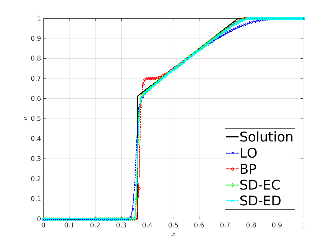
(a) RP1 at $t=1.0$, no fully discrete entropy fixes

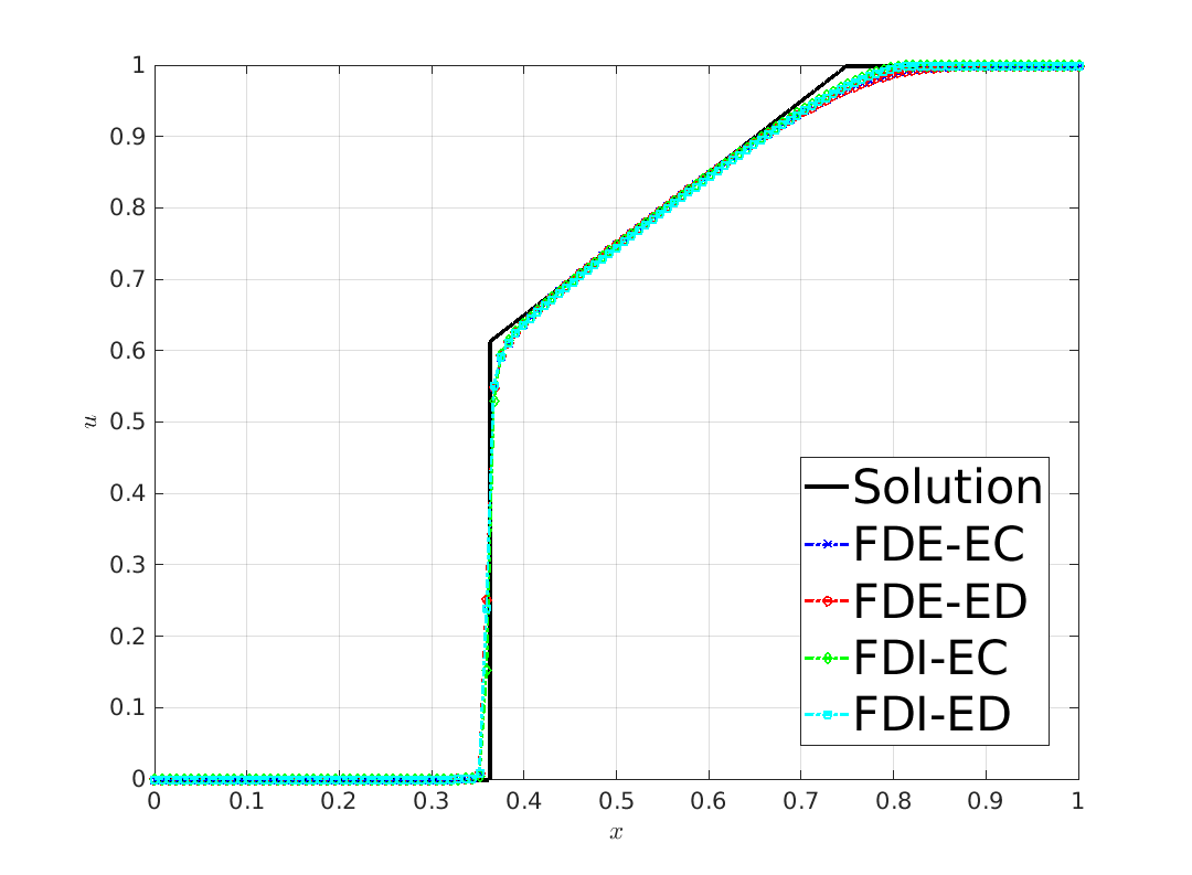
(b) RP1 at $t=1.0$ with fully discrete entropy fixes

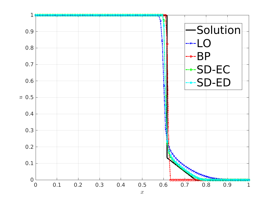
(c) RP2 at $t=2.0$, no fully discrete entropy fixes

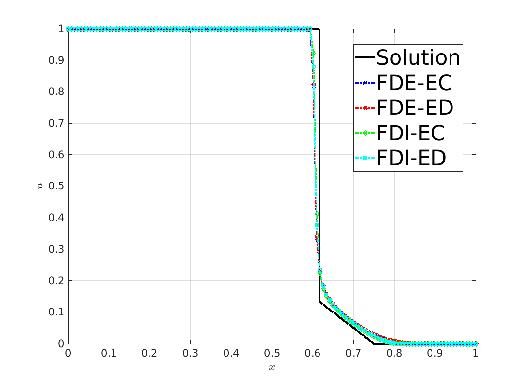
(d) RP2 at $t=2.0$ with fully discrete entropy fixes

Figure 1: 1D KPP problem, numerical solutions of RP1 and RP2 calculated with LO, BP, SD, and FD schemes on a uniform mesh of $\mathbb{P}_{1}$ finite elements using $h=\frac{1}{128}$ and $\Delta t=5\cdot 10^{-3}$. The acronyms used in the caption and legends are defined at the beginning of Section 6.

6.2 Two-dimensional KPP equation

The two-dimensional KPP problem [18, 19, 26] is a particularly challenging test for high-order numerical schemes. Equation (2.1a) with the nonconvex flux function

$$\mathbf{f}(u)=(\sin(u),\cos(u))$$ (6.2)

is solved in the computational domain $\Omega_{h}=(-2,2)\times(-2.5,1.5)$ using the initial condition

$$u_{0}(x,y)=\begin{cases}\frac{7\pi}{2}&\mbox{if}\quad\sqrt{x^{2}+y^{2}}\leq 1,\\ \frac{\pi}{4}&\mbox{otherwise}.\end{cases}$$ (6.3)

The entropy flux corresponding to the square entropy $\eta(u)=\frac{u^{2}}{2}$ is given by

$$\mathbf{q}(u)=(u\sin(u)+\cos(u),u\cos(u)-\sin(u)).$$

The maximum wave speed is bounded by $\lambda=1$. We use this value in formula (3.2) for the artificial viscosity coefficients $d_{ij}$. More accurate estimates can be found in [19].

The entropy solution of the KPP problem exhibits a two-dimensional rotating wave structure. The main challenge of this test is to avoid convergence to wrong weak solutions. All results displayed in Figs 3–4 were calculated on a uniform mesh of $128\times 128$ bilinear finite elements using the time step $10^{-3}$ and the final time $t=1.0$. The oscillatory and qualitatively incorrect numerical solution shown in Fig. 3(a) was produced by the high-order baseline scheme, i.e., (2.11) with $\alpha_{ij}=1$ and $f_{ij}^{*}=f_{ij}$ defined by (6.1). The low-order approximation shown in Fig. 3(b) was obtained with $\alpha_{ij}=0$. It reproduces the rotating wave structure of the entropy solution correctly (cf. [19, 32]) but is very diffusive. The result of bound-preserving MCL flux correction without entropy fixes is presented in Fig. 3(c). There are no spurious oscillations but the AFC scheme converges to a wrong weak solution.

In the next series of numerical experiments, we apply the entropy correction factors $\alpha_{ij}$ to the unconstrained target fluxes $f_{ij}^{*}=f_{ij}$, i.e., we deactivate the bound-preserving (BP) flux limiter to study the effect of limiter-based entropy stabilization separately. The results are shown in Fig. 3. It can be seen that entropy-conservative (EC) fixes are insufficiently dissipative, while their entropy-dissipative (ED) counterparts perform well. The numerical solutions presented in Fig. 4 demonstrate that BP flux limiting eliminates undershoots and overshoots but convergence to a wrong weak solution is possible if the EC bound is used in the entropy fix. The nonoscillatory approximations produced by the BP-ED versions of the SD, FDE, and FDI schemes preserve the wave structure of the entropy-stable LO result and are less diffusive. In this example, no significant differences are observed between the outcomes of semi-discrete and fully discrete fixes based on the same definition of $Q_{ij}$.

To study the convergence behavior of different algorithms for a nonlinear problem with a smooth exact solution, we replace the discontinuous initial condition (6.3) by

$$u_{0}(x,y)=\begin{cases}\frac{\pi}{4}\left(1+\frac{1}{20}\left(1+\cos(\pi\sqrt{x^{2}+y^{2}}\right)\right)&\mbox{if}\quad\sqrt{x^{2}+y^{2}}\leq 1,\\ \frac{\pi}{4}&\mbox{otherwise}\end{cases}$$ (6.4)

and determine the experimental order of convergence (EOC) for $h=\frac{1}{256}$ using the formula

$$\mathrm{EOC}=\frac{\log\left(\frac{\|u_{4h}-u_{2h}\|}{\|u_{2h}-u_{h}\|}\right)}{\log 2}.$$

(a) HO

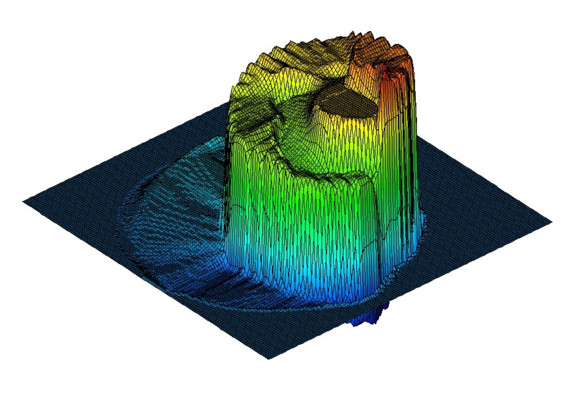
(b) LO

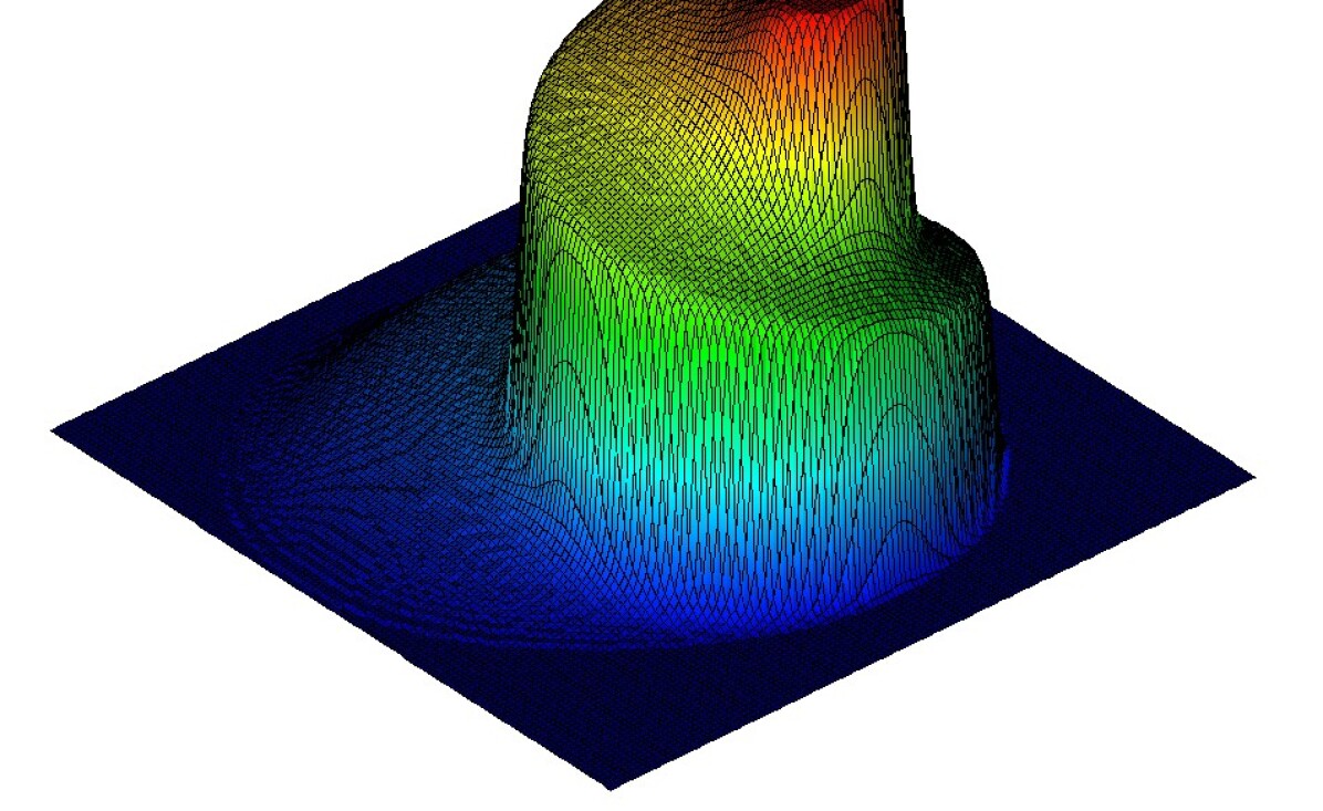
(c) BP

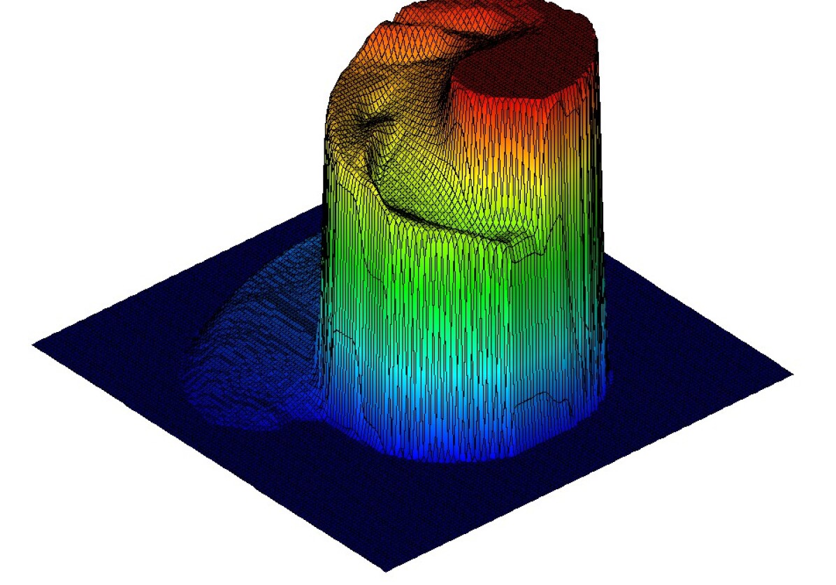
Figure 2: KPP problem with initial condition (6.3), (a) high-order, (b) low-order, and (c) flux-corrected $\mathbb{Q}_{1}$ approximations at $t=1.0$ calculated on a uniform mesh using $h=\frac{1}{128}$, $\Delta t=10^{-3}$ without entropy fixes.

(a) SD-EC

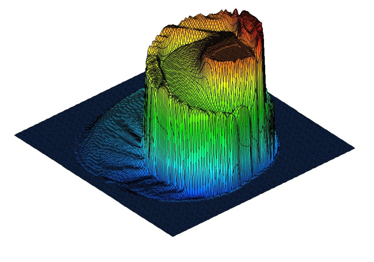
(b) FDE-EC

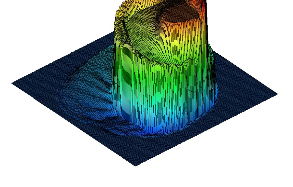
(c) SD-ED

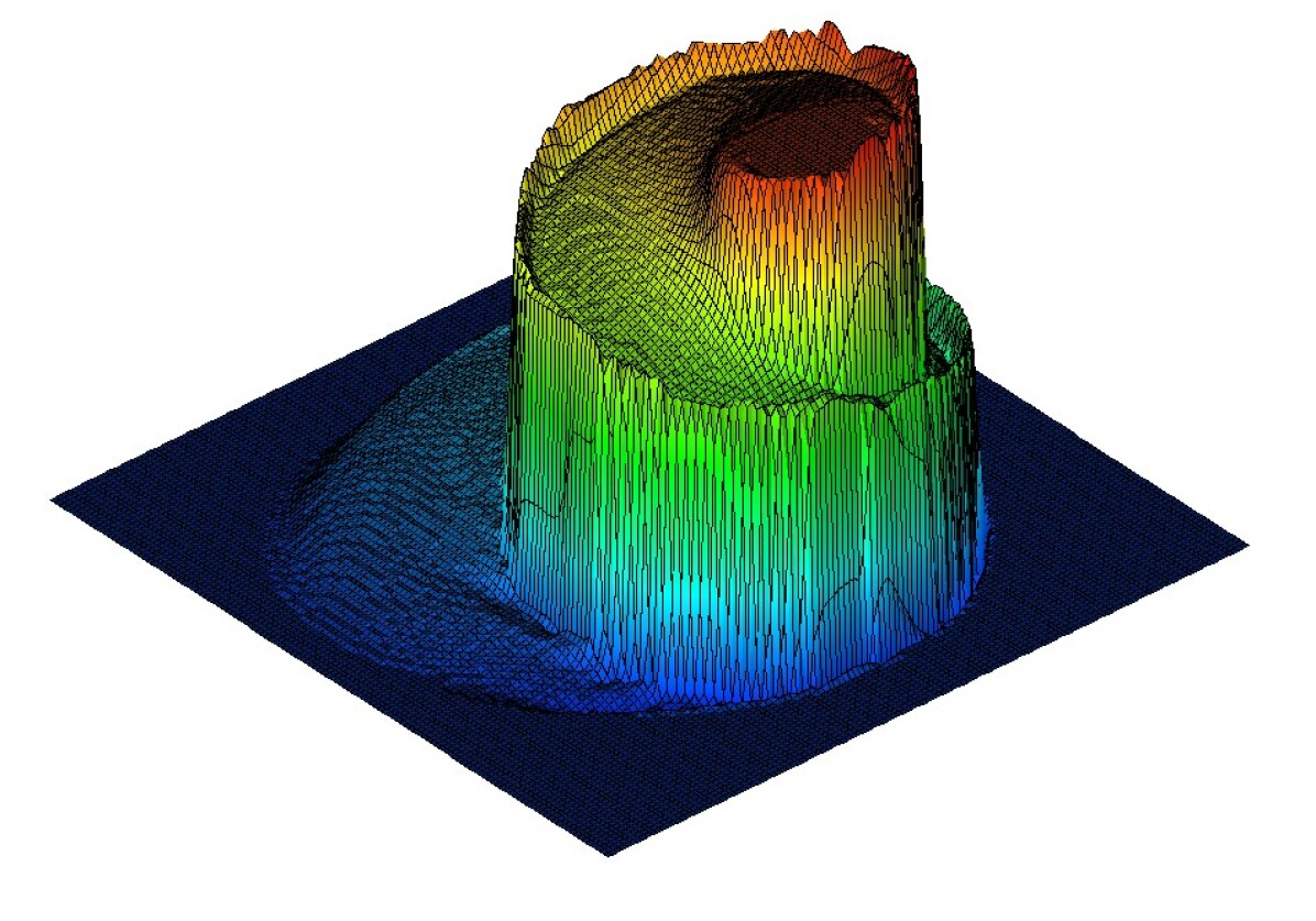
(d) FDE-ED

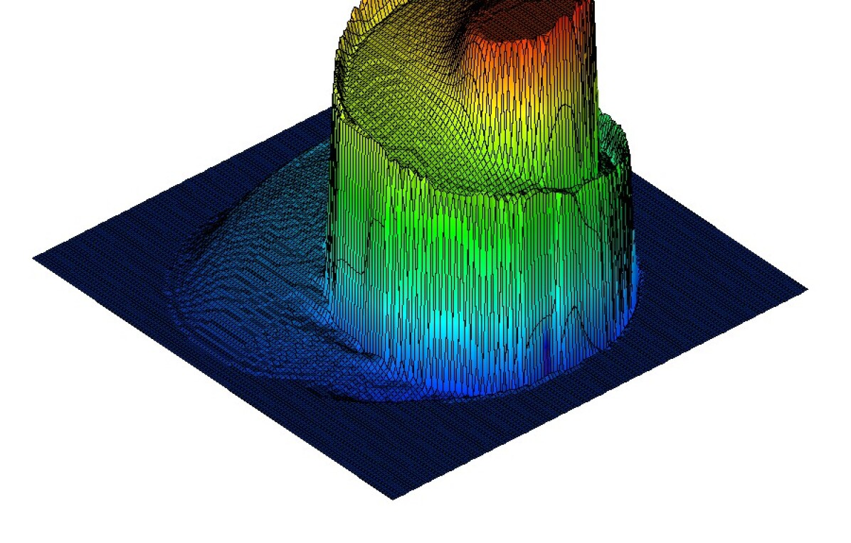
Figure 3: KPP problem with initial condition (6.3), flux-corrected $\mathbb{Q}_{1}$ approximations at $t=1.0$ calculated on a uniform mesh using $h=\frac{1}{128}$, $\Delta t=10^{-3}$ and entropy stabilization without BP limiting.

	LO	HO	BP	SD	FDE	FDI
$\mathrm{EOC}_{L^{1}}$	0.75	2.28	2.39	2.40	1.28	2.13
$\mathrm{EOC}_{L^{2}}$	0.71	2.06	2.25	2.30	1.24	2.11

Table 1: KPP problem with initial condition (6.4), $L^{1}$ and $L^{2}$ convergence rates.

(a) SD-EC

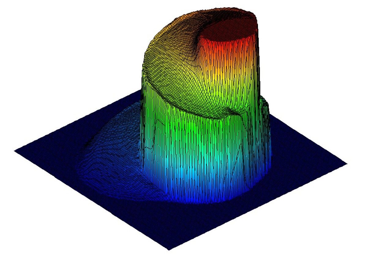
(b) FDE-EC

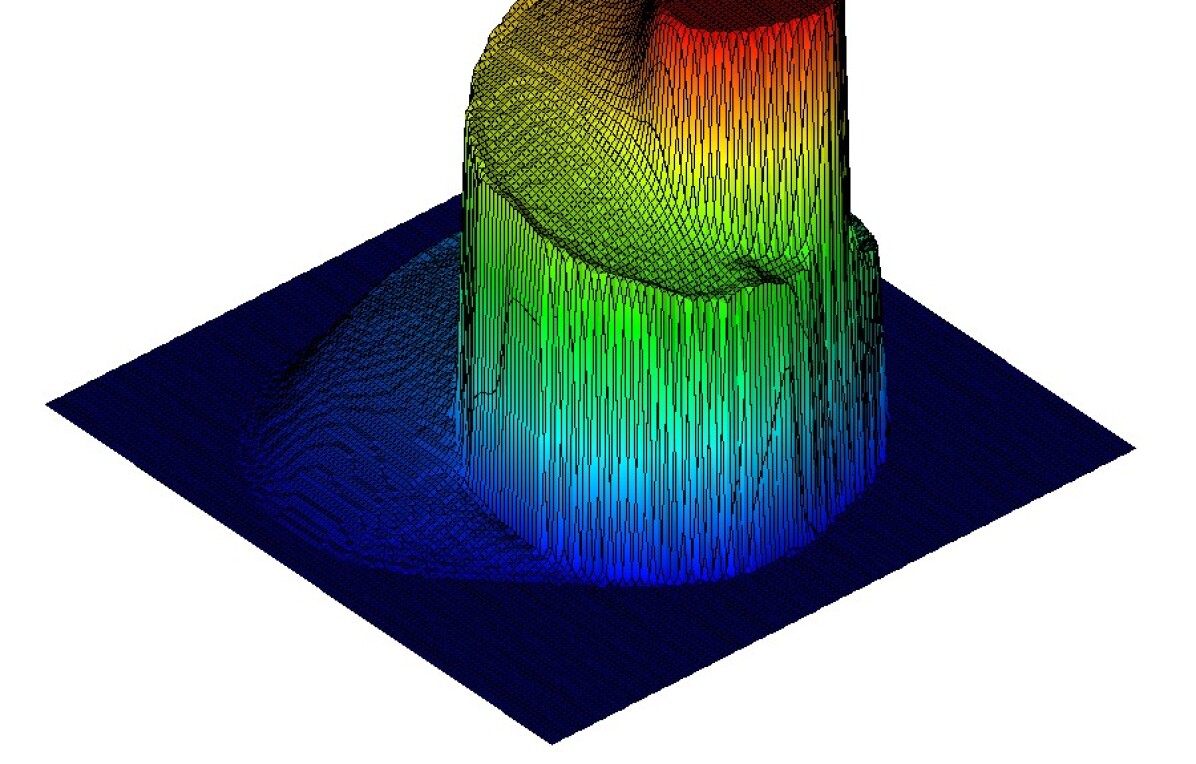
(c) FDI-EC

(d) SD-ED

(e) FDE-ED

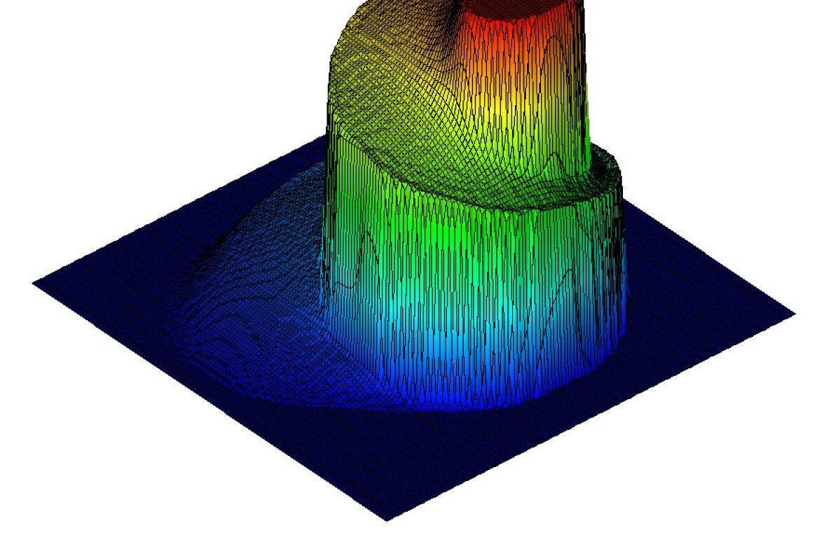
(f) FDI-ED

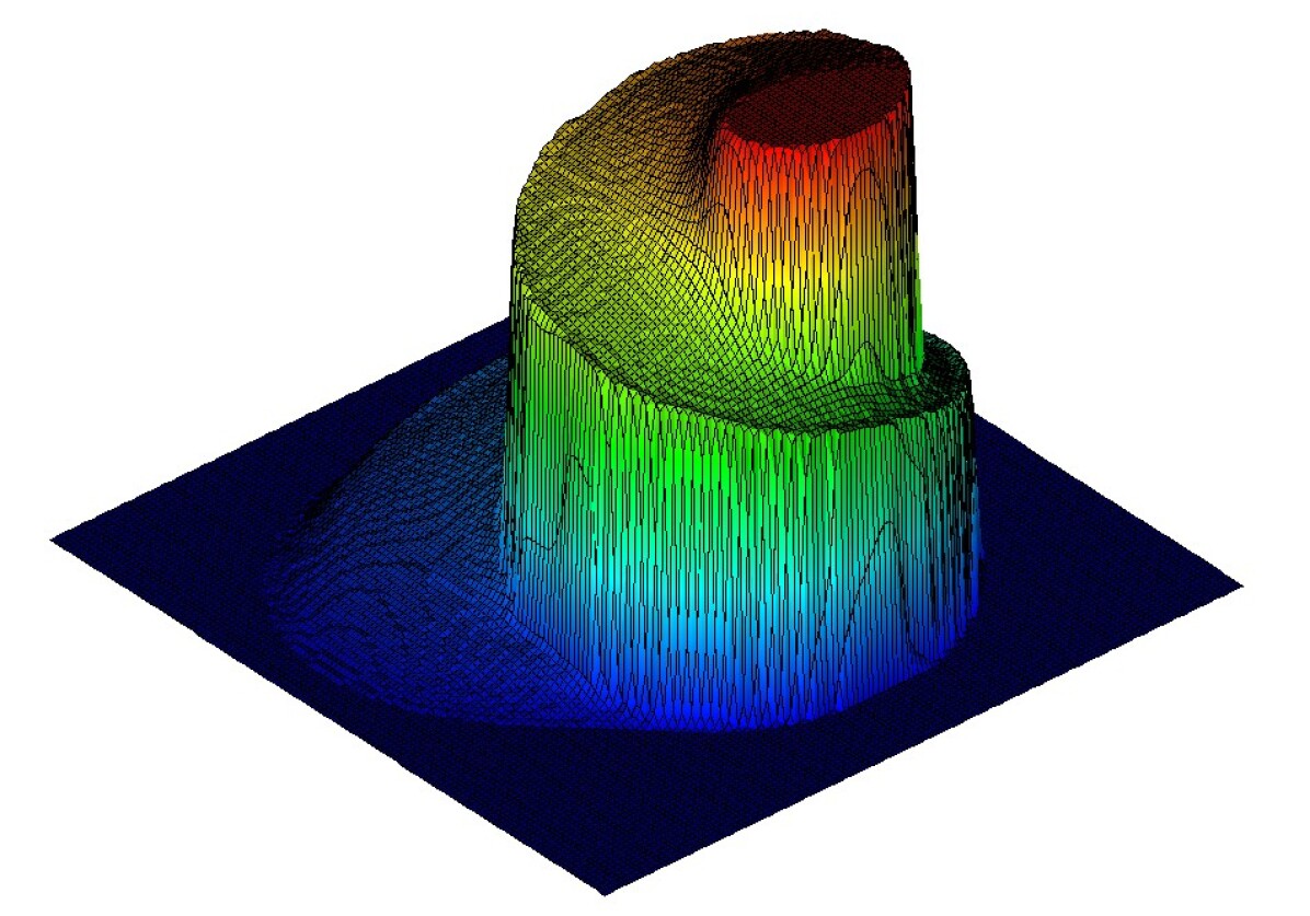
Figure 4: KPP problem with initial condition (6.3), flux-corrected $\mathbb{Q}_{1}$ approximations at $t=1.0$ calculated on a uniform mesh using $h=\frac{1}{128}$, $\Delta t=10^{-3}$ and entropy stabilization with BP limiting.

In the process of mesh refinement, we keep the ratio $\frac{\Delta t}{h}=0.256$ fixed. The rates of convergence w.r.t. discrete $L^{1}$ and $L^{2}$ norms are reported in Table 1. In this experiment, all entropy fixes use BP prelimiting and the ED bound defined by (4.7). The EOC of the unconstrained HO scheme is slightly higher than 2 due to superconvergence of consistent-mass approximations using linear or bilinear finite elements. The BP, SD, and FDI algorithms preserve second-order accuracy. The first-order convergence behavior of the FDE version is caused by the failure of stagewise explicit fixes to exploit cancellation of entropy production and dissipation in high-order Runge–Kutta schemes (see Remark 8). If the time step is chosen so that $\frac{\Delta t}{h^{2}}=128^{2}\cdot 10^{-3}$ remains fixed, the FDE version delivers $\mathrm{EOC}_{L^{1}}$=1.95 and $\mathrm{EOC}_{L^{2}}$=1.85. To achieve second-order accuracy without using $\Delta t=\mathcal{O}(h^{2})$, the entropy correction factors of the FDE fix could be redefined as

$$\alpha_{ij}=\max\{1-\max\{\beta_{i},\beta_{j}\},\min\{R_{i},R_{j}\}\},$$

where $\beta_{i}\in[0,1]$ is a smoothness indicator such as the entropy residual sensor used in [31] to stabilize the target flux as originally proposed in [17]. The FDI fix can also be configured to use $\alpha_{ij}\geq 1-\max\{\beta_{i},\beta_{j}\}$. In this way, the use of fully discrete fixes can be restricted to subdomains with large entropy residuals and the cost of calculating $\alpha_{ij}$ can be reduced.

To compare our new approaches with an existing FD fix, we used the method of Berthon et al. [5, 6] to construct localized artificial viscosities $d_{ij}^{\mathrm{FD}}$ for the entropy-corrected fluxes $\alpha_{ij}f_{ij}^{*}+d_{ij}^{\mathrm{FD}}(u_{j}-u_{i})$, where $\alpha_{ij}$ is the correction factor of the semi-discrete entropy fix (4.6). In our AFC notation, the formula for $d_{ij}^{\mathrm{FD}}$ is given by (cf. [6, eq.(12)–(14)])

$$d_{ij}^{\mathrm{FD}}=\begin{cases}-\frac{P_{ij}}{2D_{ij}}&\mbox{if}\ P_{ij}D_{ij}<0,\\ 0&\mbox{otherwise},\end{cases}$$ (6.5)

$$P_{ij} =d_{ij}[\eta(u_{j}^{*})+\eta(u_{i}^{*})-\eta(u_{j})+\eta(u_{i})]+(\mathbf{q}_{j}-\mathbf{q}_{i})\cdot\mathbf{c}_{ij},$$

$$D_{ij} =2\eta\left(\frac{u_{j}+u_{i}}{2}\right)-\eta(u_{j})-\eta(u_{i}),$$

$$u_{j}^{*} =u_{j}-\frac{(\mathbf{f}_{j}-\mathbf{f}_{i})\cdot\mathbf{c}_{ij}+d_{ij}(u_{j}-u_{i})+\alpha_{ij}f_{ij}^{*}}{2d_{ij}},$$

$$u_{i}^{*} =u_{i}-\frac{(\mathbf{f}_{j}-\mathbf{f}_{i})\cdot\mathbf{c}_{ij}-d_{ij}(u_{j}-u_{i})-\alpha_{ij}f_{ij}^{*}}{2d_{ij}}.$$

Note that $u_{j}^{*}+u_{i}^{*}=2\bar{u}_{ij}$ and $D_{ij}\leq 0$ since $\eta(u)$ is convex. The analysis in [5, 6] is restricted to 1D and assumes that the same global value of $d_{ij}^{\mathrm{FD}}$ is used for all fluxes. Hence, the multidimensional generalization (6.5) may fail to enforce fully discrete entropy stability. Nevertheless, it provides an interesting alternative to the limiter-based FDE fix.

Lemma 2 in [6] ensures that $d_{ij}^{\mathrm{FD}}=\gamma d_{ij}$, where $\gamma=\mathcal{O}(1)$, for target fluxes of the form $f_{ij}=d_{ij}(u_{i}-u_{j})$. However, the ones defined by (6.1) do not necessarily vanish if $u_{i}=u_{j}$. As a consequence, $\gamma$ can become unbounded or large enough to violate the CFL condition. For that reason, we use $d_{ij}$ defined by (3.2) as upper bound for $d_{ij}^{\mathrm{FD}}$ in the consistent-mass version. The results for the KPP problem with the discontinuous initial condition (6.3) are similar to those obtained with the FDE fix (not shown here). As expected, the artificial viscosity method also exhibits first-order convergence ($\mathrm{EOC}_{L^{1}}=0.98$, $\mathrm{EOC}_{L^{2}}$=0.95) in the smooth KPP test with the initial condition (6.4) and $\frac{\Delta t}{h}=0.256$ refinements.

6.3 One-dimensional shallow water equations

Having studied the KPP problem in the one- and two-dimensional setting, we now move on to the case of 1D systems of conservation laws. First, we consider the shallow water equations. In the case of a flat bottom topography, this hyperbolic system reads

$$\frac{\partial}{\partial t}\begin{bmatrix}h\\ hv\end{bmatrix}+\frac{\partial}{\partial x}\begin{bmatrix}hv\\ hv^{2}+\frac{g}{2}h^{2}\end{bmatrix}=0.$$

Here $h$ is the total water height, $v$ is the depth-integrated velocity, and $g$ is the gravitational acceleration, which we set equal to 1. An entropy-entropy flux pair and the corresponding entropy potential for the shallow water system are given by [9, 14]

$$\eta(u)=\frac{1}{2}(hv^{2}+gh^{2}),\qquad q(u)=\frac{1}{2}hv^{3}+gh^{2}v,\qquad\psi(u)=\frac{1}{2}gh^{2}v.$$

We test the numerical behavior of the proposed flux correction methods for a wet dam break example corresponding to the initial condition

$$u_{0}(x)=\begin{cases}(1,0)&\mbox{if }x<0,\\ (0.1,0)&\mbox{otherwise.}\end{cases}$$ (6.6)

In this Riemann problem, two water columns of different height are initially separated by a dam, which is removed at the start of the simulation. After the dam break, the higher water column expands into a rarefaction fan, and a shock front propagates into the lower water level region. The height of the plateau between the shock and the rarefaction wave is given by $c_{m}^{2}/g$, where $c_{m}$ is a root of a sixth-degree polynomial. For the particular initial condition (6.6), we use the value $c_{m}\approx 0.6294$ to approximate the analytical solution of this problem as in [11] (the expressions in the journal version of this reference are incorrect).

We simulate the dam break in the computational domain $\Omega=(-0.5,0.5)$ and impose reflecting wall boundary conditions at $x=\pm 0.5$. The final time is $t=0.3$. To compare the accuracy of individual approaches, we run simulations on a sequence of successively refined uniform meshes using the time step $\Delta t=0.25h$. The scalar quantity of interest

$$e_{1}(t)=\|u(t)-u_{h}(t)\|_{L^{1}(\Omega)^{2}}$$

is defined as the sum of $L^{1}(\Omega)$ errors in the conserved variables. It measures the accuracy of a given approximation at $t\geq 0$. The values of $e_{1}(0.3)$ and the corresponding EOCs are summarized in Tables 2 and 3. Because of the discontinuity in (6.6), first-order accuracy of the BP scheme equipped with the Galerkin target flux is optimal. The semi-discrete entropy fix using either (4.5) or (4.7) does not degrade the rate of convergence. The high-resolution GT versions of the BP, SD, and FD approaches are clearly superior to the low-order method, which is significantly more diffusive. All numerical results obtained with the Roe target flux are also less accurate than the corresponding Galerkin approximations.

It is well known that Roe’s scheme applied to the Euler equations can produce nonphysical stationary shocks at sonic points [3, 8, 12, 43, 54]. The same is true for the shallow water equations [22, 24]. In fact, an entropy-violating shock can form even in our simple example. To show this and study the convergence behavior of GT-BP, RT-BP, RT-SD, and RT-FDE approximations, we performed a sequence of simulations with increased spatial and temporal resolution. The results for the water height are shown in Fig. 5. Since the errors and EOCs in Tables 2 and 3 indicate that EC and ED versions of entropy fixes perform similarly for this benchmark, we only show the results obtained with entropy-conservative bounds. The use of Galerkin target fluxes produces profiles that are in very good agreement with the analytical solution, while solutions for Roe target fluxes exhibit small nonphysical shocks within the rarefaction wave region. The semi-discrete entropy fix reduces the magnitude of spurious jumps but only the additional fully discrete fix produces qualitatively correct profiles.

$E_{h}$	LO	EOC	GT-BP	EOC	GT-SD-EC	EOC	GT-SD-ED	EOC
32	1.38E-01		5.99E-02		6.50E-02		6.57E-02
64	8.43E-02	0.71	3.16E-02	0.92	3.42E-02	0.93	3.46E-02	0.92
128	4.98E-02	0.76	1.61E-02	0.98	1.75E-02	0.97	1.77E-02	0.97
256	2.91E-02	0.78	8.19E-03	0.97	8.88E-03	0.98	8.99E-03	0.98

Table 2: Wet dam break with initial condition (6.6), convergence history for $e_{1}(0.3)$ and corresponding EOCs of low- and high-order schemes using Galerkin target fluxes.

$E_{h}$	RT-BP	EOC	RT-SD	EOC	RT-FD-EC	EOC	RT-FD-ED	EOC
32	1.33E-01		1.33E-01		1.33E-01		1.33E-01
64	7.90E-02	0.75	7.90E-02	0.75	7.97E-02	0.74	7.97E-02	0.74
128	4.57E-02	0.79	4.57E-02	0.79	4.62E-02	0.79	4.62E-02	0.79
256	2.62E-02	0.80	2.61E-02	0.81	2.65E-02	0.80	2.65E-02	0.80

Table 3: Wet dam break with initial condition (6.6), convergence history for $e_{1}(0.3)$ and corresponding EOCs high-order schemes using Roe target fluxes.

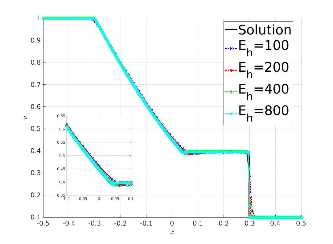
(a) GT-BP

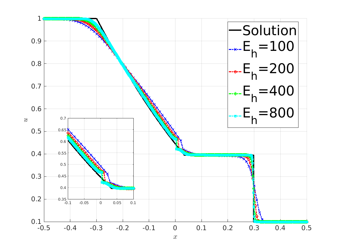
(b) RT-BP

(c) RT-SD

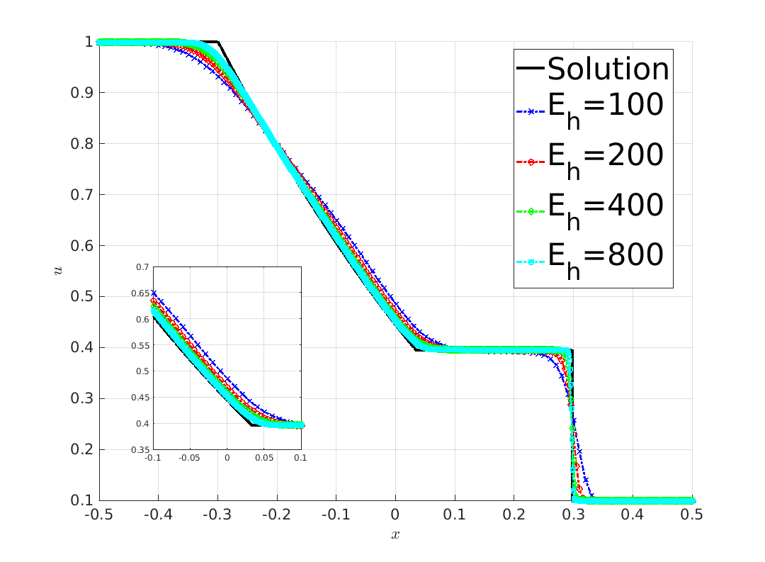
(d) RT-FDE

Figure 5: Vanishing viscosity solution and approximations to the water height of the wet dam break with initial condition (6.6). Results at $t=0.3$ on four refinement levels using $\Delta t=0.25h$.

6.4 One-dimensional Euler equations of gas dynamics

Another hyperbolic model of particular importance are the Euler equations of gas dynamics. In the 1D case, this system of conservation laws reads

$$\frac{\partial}{\partial t}\begin{bmatrix}\varrho\\ \varrho v\\ \varrho E\end{bmatrix}+\frac{\partial}{\partial x}\begin{bmatrix}\varrho v\\ \varrho v^{2}+p\\ (\varrho E+p)v\end{bmatrix}=0,$$

where $\varrho$ is the fluid density, $v$ is the velocity, and $E$ is the specific total energy. The pressure $p$ of a polytropic ideal gas is given by the equation of state

$$p(u)=(\gamma-1)\left(\varrho E-\frac{\varrho v^{2}}{2}\right)$$

in which $\gamma$ denotes the adiabatic constant. For diatomic gases and air, $\gamma$ is approximately equal to $1.4$. We use this value in our simulations. An entropy-entropy flux pair and the corresponding entropy potential for the Euler system are given by [9, 21]

$$\eta(u)=\frac{\varrho s(u)}{1-\gamma},\qquad q(u)=\frac{\varrho vs(u)}{1-\gamma},\qquad\psi(u)=\varrho v,$$

where $s(u)=\log(p\varrho^{-\gamma})$ is the specific entropy. Note that $s(u)$ and $\eta(u)$ have opposite signs, since the physical entropy is concave while the mathematical one is convex.

6.4.1 Shock tube problems

In the first numerical experiment for the one-dimensional Euler equations, we solve the classical shock tube problem with Sod’s [51] initial condition

$$u_{0}(x)=\begin{cases}(1,0,2.5)&\mbox{if }x<0.5,\\ (0.125,0,0.25)&\mbox{otherwise}\end{cases}$$ (6.7)

in the computational domain $\Omega=(0,1)$ with reflecting wall boundaries. The analytical solution is qualitatively similar to that of the dam break problem considered in Section 6.3 but features a contact discontinuity in addition to the shock and rarefaction. To facilitate direct comparison with the results presented in [28], we stop simulations at $t=0.231$ and run them on a uniform mesh with $h=\frac{1}{128}$ using the constant time step $\Delta t=10^{-3}$.

For this simple test problem, all high-resolution schemes based on the same definition of the target flux produce similar results. That is why only numerical solutions obtained with the GT and RT versions of the SD-EC algorithm are compared in Fig. 6. The GT profiles are very similar to the ones obtained without the semi-discrete entropy fix (cf. Fig. 4(a) in [28]) and less diffusive than the corresponding RT approximations. In this example, all approaches produce qualitatively correct results which converge to the entropy solution.

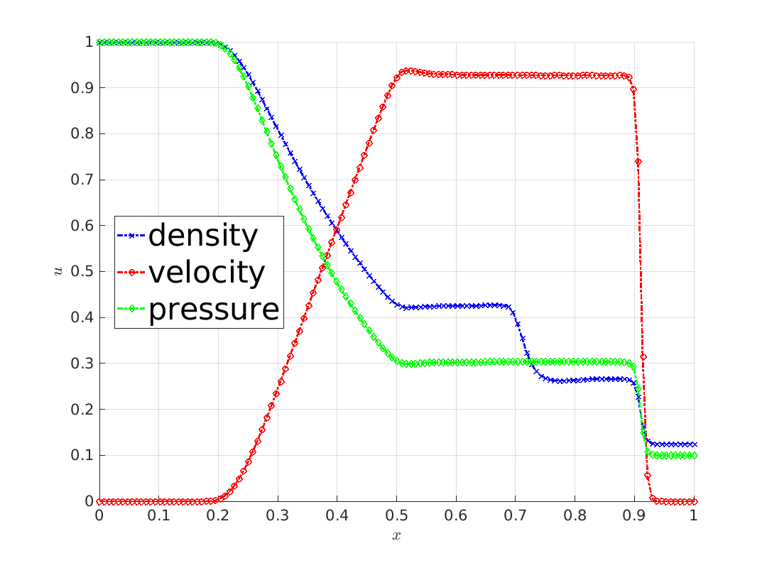
(a) GT-SD-EC

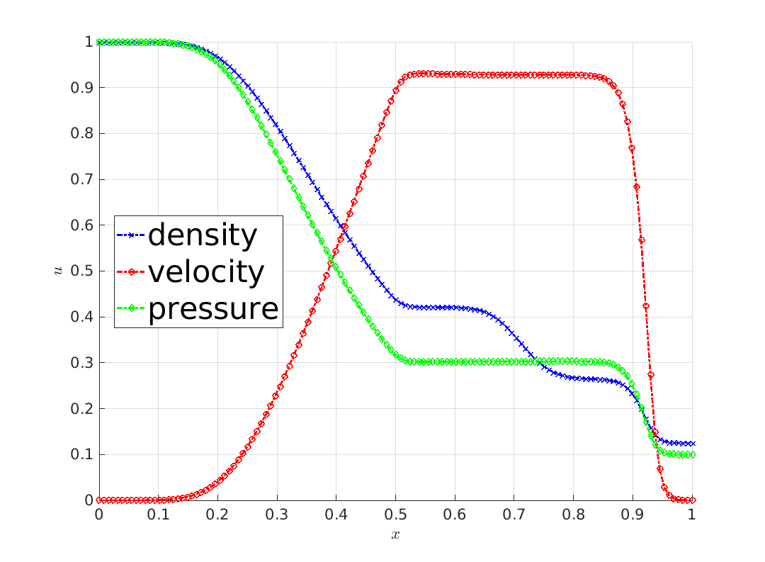
(b) RT-SD-EC

Figure 6: Sod’s shock tube [51], primitive variables at $t=0.231$ calculated on a uniform mesh with $h=\frac{1}{128}$ and $\Delta t=10^{-3}$. The SD-EC scheme constrains the Galerkin or Roe target flux using bound-preserving convex limiting and the semi-discrete entropy fix with EC bounds (4.5).

Let us now repeat the above shock tube experiment using the initial condition

$$u_{0}(x)=\begin{cases}(1,0.75,89/32)&\mbox{if }x<0.3,\\ (0.125,0,0.25)&\mbox{otherwise}.\end{cases}$$ (6.8)

The Riemann problem with this initial data is known as modified Sod’s shock tube [54] and is specifically designed to have a sonic point within the rarefaction wave. Another difference to the classical shock tube problem is that the left boundary is now an inlet.

The results in Fig. 7 depict approximations to the primitive variables $\varrho,v$, and $E$ at $t=0.2$. No entropy fixes are used for Galerkin target fluxes. As in the dam break example, the GT-BP results are qualitatively correct, so there is no need for entropy correction. Although Roe’s scheme without an entropy fix is considerably more diffusive, it produces an entropy shock at the sonic point, as in the case of the shallow water equations. The semi-discrete fix reduces the magnitude of the spurious jump, and the resulting approximations do converge to the correct solution as the mesh and time step are refined. However, only the fully discrete fix prevents formation of the entropy shock already on coarse meshes.

(a) GT-BP

(b) RT-BP

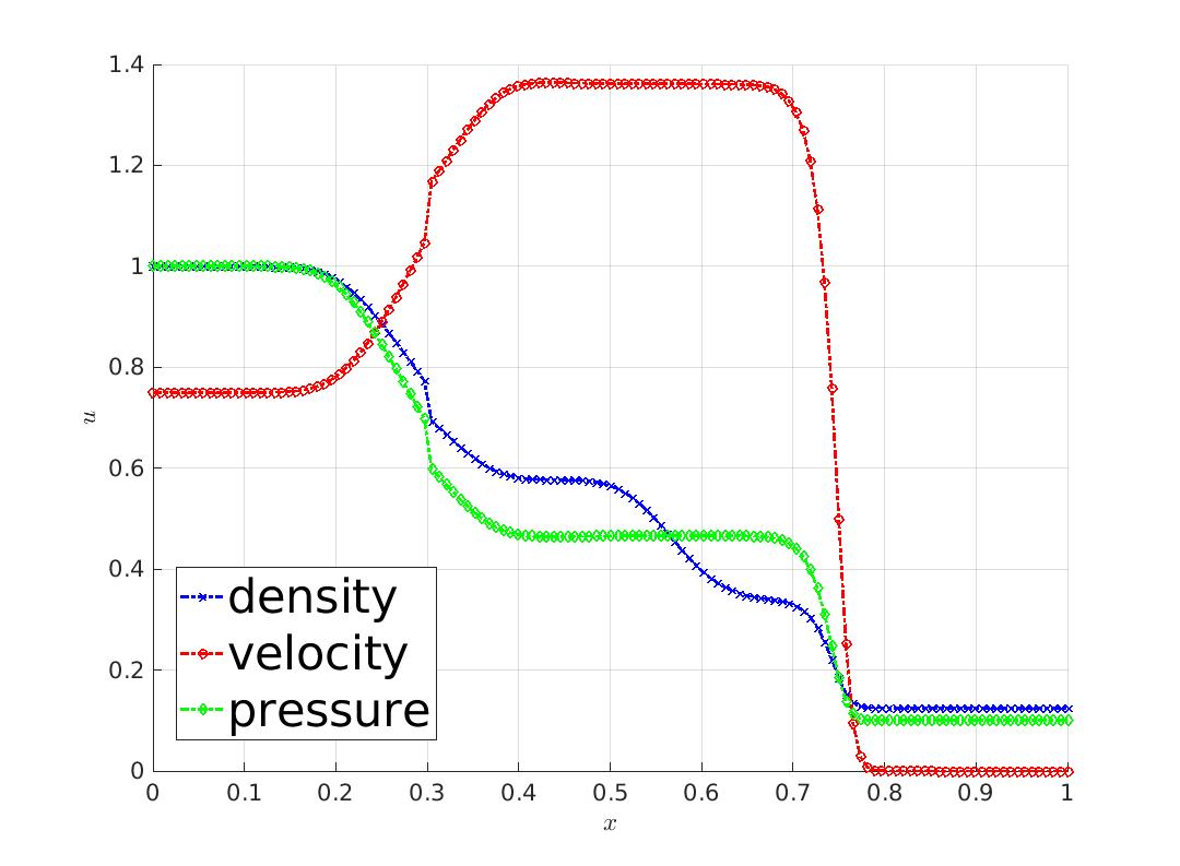
(c) RT-SD-ED

(d) RT-FDE-ED

Figure 7: Modified Sod’s shock tube [54], primitive variables at $t=0.2$ calculated on a uniform mesh with $h=\frac{1}{128}$ and $\Delta t=10^{-3}$. No entropy fix is performed in the BP version. The SD and FDE entropy fixes for Roe target fluxes use ED bounds (4.7).

6.4.2 Other benchmarks for the Euler equations

Among the benchmarks considered so far, only the 1D and 2D KPP problems did require entropy fixes for BP schemes using Galerkin fluxes. Indeed, all GT results for hyperbolic systems were qualitatively correct. While the semi-discrete fix did not significantly increase the levels of diffusivity, the fully discrete explicit fix did but was found to be a better cure for entropy shocks generated by Roe target fluxes. To show that this behavior is not unique to the problems considered in Section 6.3 and Section 6.4.1, we apply the GT-BP, GT-SD, RT-BP and RT-FDE methods to four additional 1D benchmarks for the Euler equations. The resulting density approximations are presented in Fig. 8. For a detailed description and setup of each test problem, we refer the reader to the references cited below.

The diagram in Fig. 8(a) shows the results for the final test in [12, Sec. 6 A]. We remark that the parameter $c_{R}$ in the setup of this problem is left unspecified in the reference. Based on the results presented in [12], we use $c_{R}=4$. The results in Figs. 8(b) and 8(c) correspond to test cases 1 and 2 in [43]. The problem solved in Fig. 8(d) is the classical Shu–Osher sine-shock interaction [50]. Again, approximations obtained with Galerkin target fluxes are free of artifacts, and their accuracy is not affected by the optional semi-discrete fix. The use of Roe target fluxes makes the baseline scheme more diffusive and entropy unstable but the latter deficiency can be cured by applying a limiter-based entropy fix. This study confirms our previous observations that, in practice, the semi-discrete entropy fix for Galerkin fluxes is sufficient to avoid convergence to entropy-violating weak solutions. It does not degrade the overall accuracy and even the entropy-conservative version converges to the vanishing viscosity solution, while reducing the magnitude of spurious jumps on coarse meshes. The fully discrete explicit fix makes it possible to suppress nonphysical effects completely but introduces additional numerical dissipation. Remarkably, the methods under investigation exhibit this behavior for all conservation laws and initial data considered in this work.

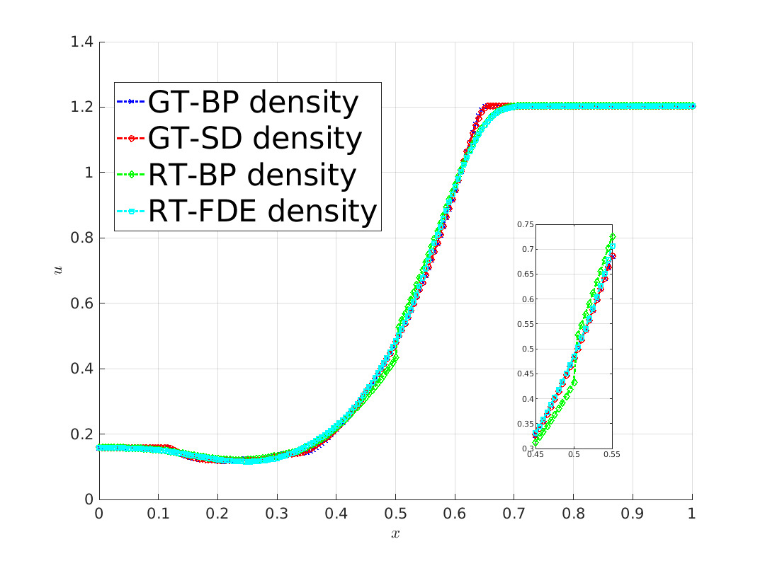
(a) [12], $E_{h}=200,\leavevmode\nobreak\ \Delta t=4\cdot 10^{-4}$

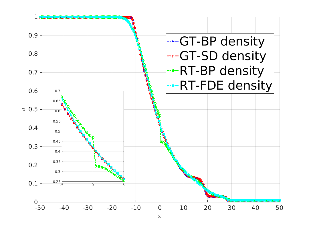
(b) [43], $E_{h}=200,\leavevmode\nobreak\ \Delta t=4\cdot 10^{-4}$

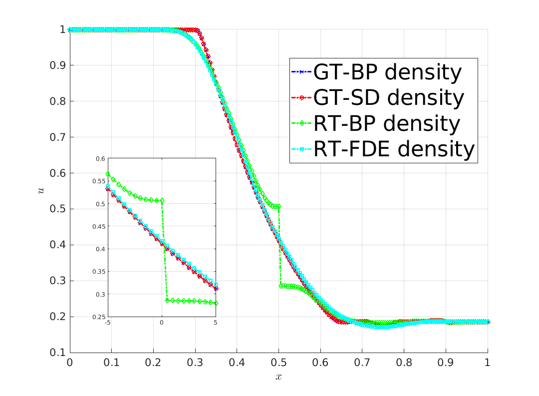
(c) [43], $E_{h}=200,\leavevmode\nobreak\ \Delta t=5\cdot 10^{-6}$

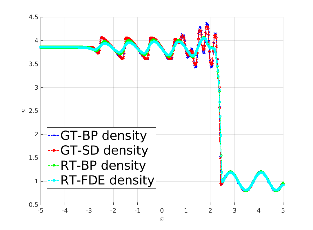
(d) [50], $E_{h}=500,\leavevmode\nobreak\ \Delta t=2\cdot 10^{-3}$

Figure 8: Density profiles of the GT-BP, GT-SD, RT-BP, and RT-FDE solutions to the 1D Euler equations for standard test problems referenced in the text of Section 6.4.2.

7 Conclusions

The main outcome of this work is a general framework for constraining a continuous finite element approximation to satisfy entropy stability conditions. Combining a property-preserving algebraic Lax–Friedrichs method with a high-order target scheme, we designed algebraic flux correction procedures that ensure not only preservation of invariant domains but also validity of local entropy inequalities. The semi-discrete entropy production limiter proposed in [31] was extended to systems and fully discrete schemes. The results of our numerical experiments indicate that a semi-discrete entropy fix is usually sufficient for convergence to correct weak solutions if the underlying inequality constraints are formulated using a dissipative bound for entropy production by antidiffusive fluxes. The fully discrete explicit fix for forward Euler stages of an SSP Runge–Kutta method was found to stabilize an entropy-conservative space discretization but degrade the rate of convergence to smooth solutions. As an alternative, we proposed an implicit iterative fix for the final stage of a general Runge–Kutta method. In terms of accuracy, this algorithm performs similarly to the semi-discrete fix for RK stages. However, fully discrete entropy stability is required by the presented generalization of the Lax–Wendroff theorem to finite elements. Hence, it is at least a desirable theoretical property which may need to be enforced if the baseline scheme is highly unstable. The Galerkin group approximation considered in this work is almost entropy conservative for $\mathbb{P}_{1}$ and $\mathbb{Q}_{1}$ finite elements. For such target schemes, the benefits of a fully discrete fix may not be worth the effort. The entropy-conservative version of our semi-discrete fix has already been extended to high-order continuous finite element discretizations of scalar conservation laws in [32], while a high-order DG version of the bound-preserving MCL limiter without entropy fixes was developed in [20]. We envisage that entropy stability of such high-order AFC schemes can also be enforced using the proposed methodology.

References

- [1] R. Abgrall (2018) A general framework to construct schemes satisfying additional conservation relations. Application to entropy conservative and entropy dissipative schemes J. Comput. Phys. 372: 640–666 doi: 10.1016/j.jcp.2018.06.031
- [2] R. Abgrall, P. Öffner, H. Ranocha (2019) Reinterpretation and extension of entropy correction terms for residual distribution and discontinuous Galerkin schemes Preprint, arXiv:1908.04556v3 [math.NA]
- [3] J. W. Banks, W. D. Henshaw, J. N. Shadid (2009) An evaluation of the FCT method for high-speed flows on structured overlapping grids J. Comput. Phys. 228: 5349–5369 doi: 10.1016/j.jcp.2009.04.033
- [4] G. R. Barrenechea, P. Knobloch (2017) Analysis of a group finite element formulation Appl. Numer. Math. 118: 238–248 doi: 10.1016/j.apnum.2017.03.008
- [5] C. Berthon, M. J. Castro Díaz, , A. Duran, T. Morales de Luna, K. Saleh (2021) Artificial viscosity to get both robustness and discrete entropy inequalities Preprint, http://math.univ-lyon1.fr/~saleh/papers/Artificial-Viscosity.pdf
- [6] C. Berthon, A. Duran, K. Saleh (2020) An easy control of the artificial numerical viscosity to get discrete entropy inequalities when approximating hyperbolic systems of conservation laws. in G. V. Demidenko, E. Romenski, E. Toro, M. Dumbser (eds.), Continuum Mechanics, Applied Mathematics and Scientific Computing: Godunov’s Legacy 29–36 Springer Nature Switzerland AG doi: 10.1007/978-3-030-38870-6_5
- [7] M. H. Carpenter, T. C. Fisher, E. J. Nielsen, S. H. Frankel (2014) Entropy stable spectral collocation schemes for the Navier–Stokes equations: Discontinuous interfaces SIAM J. Sci. Comput. 36: B835–B867 doi: 10.1137/130932193
- [8] P. Chandrashekar (2013) Kinetic energy preserving and entropy stable finite volume schemes for compressible Euler and Navier–Stokes equations Commun. Comput. Phys. 14: 1252–1286 doi: 10.4208/cicp.170712.010313a
- [9] T. Chen, C.-W. Shu (2017) Entropy stable high order discontinuous Galerkin methods with suitable quadrature rules for hyperbolic conservation laws J. Comput. Phys. 345: 427–461 doi: 10.1016/j.jcp.2017.05.025
- [10] T. Chen, C.-W. Shu (2020) Review of entropy stable discontinuous Galerkin methods for systems of conservation laws on unstructured simplex meshes CSIAM Trans. Appl. Math. 1: 1–52 doi: 10.4208/csiam-am.2020-0003
- [11] O. Delestre, C. Lucas, P.-A. Ksinant, F. Darboux, C. Laguerre, T.-N.-T. Vo, F. James, S. Cordier (2016) SWASHES: a compilation of shallow water analytic solutions for hydraulic and environmental studies Preprint, arXiv:1110.0288v7 [math.NA]
- [12] B. Einfeldt (1988) On Godunov-type methods for gas dynamics SIAM J. Numer. Anal. 25: 294–318 doi: 10.1137/0725021
- [13] T. C. Fisher, M. H. Carpenter (2013) High-order entropy stable finite difference schemes for nonlinear conservation laws: Finite domains J. Comput. Phys. 252: 518–557 doi: 10.1016/j.jcp.2013.06.014
- [14] U. S. Fjordholm, S. Mishra, E. Tadmor (2011) Well-balanced and energy stable schemes for the shallow water equations with discontinuous topography J. Comput. Phys. 230: 5587–5609 doi: 10.1016/j.jcp.2011.03.042
- [15] C. Fletcher (1983) The group finite element formulation Comput. Method. Appl. M. 37: 225–244 doi: 10.1016/0045-7825(83)90122-6
- [16] G. J. Gassner (2013) A skew-symmetric discontinuous Galerkin spectral element discretization and its relation to SBP-SAT finite difference methods SIAM J. Sci. Comput. 35: A1233–A1253 doi: 10.1137/120890144
- [17] J.-L. Guermond, M. Nazarov, B. Popov, I. Tomas (2018) Second-order invariant domain preserving approximation of the Euler equations using convex limiting SIAM J. Sci. Comput. 40: A3211–A3239 doi: 10.1137/17M1149961
- [18] J.-L. Guermond, B. Popov (2016) Invariant domains and first-order continuous finite element approximation for hyperbolic systems SIAM J. Numer. Anal. 54: 2466–2489 doi: 10.1137/16M1074291
- [19] J.-L. Guermond, B. Popov (2017) Invariant domains and second-order continuous finite element approximation for scalar conservation equations SIAM J. Numer. Anal. 55: 3120–3146 doi: 10.1137/16M1106560
- [20] H. Hajduk (2021) Monolithic convex limiting in discontinuous Galerkin discretizations of hyperbolic conservation laws Comput. Math. Appl. 87: 120–138 doi: 10.1016/j.camwa.2021.02.012
- [21] A. Harten (1983) On the symmetric form of systems of conservation laws with entropy J. Comput. Phys. 49: 151–164 doi: 10.1016/0021-9991(83)90118-3
- [22] F. Kemm (2014) A note on the carbuncle phenomenon in shallow water simulations J. Appl. Math. Mech. 94: 516–521 doi: 10.1002/zamm.201200176
- [23] D. I. Ketcheson (2019) Relaxation Runge-Kutta Methods: Conservation and stability for Inner-Product Norms SIAM J. Numer. Anal. 57: 2850–2870 doi: 10.1137/19M1263662
- [24] D. I. Ketcheson, M. Quezada de Luna (2021) Numerical simulation and entropy dissipative cure of the carbuncle instability for the shallow water circular hydraulic jump Preprint, arXiv:2103.09664 [physics.flu-dyn]
- [25] S. Kivva (2020) Entropy stable flux correction for scalar hyperbolic conservation laws Preprint, arXiv:2004.02258 [math.NA]
- [26] A. Kurganov, G. Petrova, B. Popov (2007) Adaptive semidiscrete central-upwind schemes for nonconvex hyperbolic conservation laws SIAM J. Sci. Comput. 29: 2381–2401 doi: 10.1137/040614189
- [27] D. Kuzmin (2012) Algebraic flux correction I. Scalar conservation laws in D. Kuzmin, R. Löhner, S. Turek (eds.), Flux-Corrected Transport: Principles, Algorithms, and Applications 145–192 Springer 2nd ed. doi: 10.1007/978-94-007-4038-9_6
- [28] D. Kuzmin (2020) Monolithic convex limiting for continuous finite element discretizations of hyperbolic conservation laws Comput. Method. Appl. M. 361: 112804 doi: 10.1016/j.cma.2019.112804
- [29] D. Kuzmin, M. Möller, M. Gurris (2012) Algebraic flux correction II. Compressible flow problems in D. Kuzmin, R. Löhner, S. Turek (eds.), Flux-Corrected Transport: Principles, Algorithms, and Applications 193–238 Springer 2nd ed. doi: 10.1007/978-94-007-4038-9_7
- [30] D. Kuzmin, M. Möller, J. N. Shadid, M. Shashkov (2010) Failsafe flux limiting and constrained data projections for equations of gas dynamics J. Comput. Phys. 229: 8766–8779 doi: 10.1016/j.jcp.2010.08.009
- [31] D. Kuzmin, M. Quezada de Luna (2020) Algebraic entropy fixes and convex limiting for continuous finite element discretizations of scalar hyperbolic conservation laws Comput. Method. Appl. M. 372: 113370 doi: 10.1016/j.cma.2020.113370
- [32] D. Kuzmin, M. Quezada de Luna (2020) Entropy conservation property and entropy stabilization of high-order continuous Galerkin approximations to scalar conservation laws Comput. Fluids 213: 104742 doi: 10.1016/j.compfluid.2020.104742
- [33] D. Kuzmin, M. Quezada de Luna, D. I. Ketcheson, J. Grüll (2020) Bound-preserving convex limiting for high-order Runge–Kutta time discretizations of hyperbolic conservation laws Preprint, arXiv:2009.01133 [math.NA]
- [34] P. G. Lefloch, J.-M. Mercier, C. Rohde (2002) Fully discrete, entropy conservative schemes of arbitrary order SIAM J. Numer. Anal. 40: 1968–1992 doi: 10.1137/S003614290240069X
- [35] R. J. LeVeque (1992) Numerical methods for conservation laws Birkhäuser doi: 10.1007/978-3-0348-8629-1
- [36] C. Lohmann (2019) Physics-Compatible Finite Element Methods for Scalar and Tensorial Advection Problems Springer Spektrum doi: 10.1007/978-3-658-27737-6
- [37] C. Lohmann, D. Kuzmin (2016) Synchronized flux limiting for gas dynamics variables J. Comput. Phys. 326: 973–990 doi: 10.1016/j.jcp.2016.09.025
- [38] C. Lozano (2018) Entropy production by explicit Runge–Kutta schemes J. Sci. Comput. 76: 521–564 doi: 10.1007/s10915-017-0627-0
- [39] C. Lozano (2019) Entropy production by implicit Runge–Kutta schemes J. Sci. Comput. 79: 1832–1853 doi: 10.1007/s10915-019-00914-5
- [40] P. R. M. Lyra, K. Morgan (2002) A review and comparative study of upwind biased schemes for compressible flow computation. III: Multidimensional extension on unstructured grids Arch. Comput. Methods Eng. 9: 207–256 doi: 10.1007/BF02818932
- [41] R. Löhner (2008) Applied Computational Fluid Dynamics Techniques: An Introduction Based on Finite Element Methods John Wiley & Sons doi: 10.1002/9780470989746
- [42] M. L. Merriam (1989) An entropy-based approach to nonlinear stability NASA Technical Memorandum 10186 https://core.ac.uk/download/pdf/42824928.pdf
- [43] J.-M. Moschetta, J. Gressier (2000) A Cure for the Sonic Point Glitch Int. J. Comut. Fluid. Dyn. 13: 143–159 doi: 10.1080/10618560008940895
- [44] W. Pazner (2021) Sparse invariant domain preserving discontinuous Galerkin methods with subcell convex limiting Comput. Method. Appl. M. 382: 113876 doi: 10.1016/j.cma.2021.113876
- [45] W. Pazner, P.-O. Persson (2019) Analysis and Entropy Stability of the Line-Based Discontinuous Galerkin Method J. Sci. Comput. 80: 376–402 doi: 10.1007/s10915-019-00942-1
- [46] H. Ranocha, M. Sayyari, L. Dalcin, M. Parsani, D. I. Ketcheson (2020) Relaxation Runge–Kutta methods: Fully discrete explicit entropy-stable schemes for the compressible Euler and Navier–Stokes equations SIAM J. Sci. Comput. 42: A612–A638 doi: 10.1137/19M1263480
- [47] D. Ray, P. Chandrashekar, U. S. Fjordholm, S. Mishra (2016) Entropy stable scheme on two-dimensional unstructured grids for Euler equations Commun. Comput. Phys. 19: 1111–1140 doi: 10.4208/cicp.scpde14.43s
- [48] V. Selmin (1993) The node-centred finite volume approach: Bridge between finite differences and finite elements Comput. Methods Appl. Mech. Engrg. 102: 107–138 doi: 10.1016/0045-7825(93)90143-L
- [49] V. Selmin, L. Formaggia (1996) Unified construction of finite element and finite volume discretizations for compressible flows Int. J. Numer. Methods Eng. 39: 1–32 doi: 10.1002/(SICI)1097-0207(19960115)39:1<1::AID-NME837>3.0.CO;2-G
- [50] C.-W. Shu, S. Osher (1989) Efficient implementation of essentially non-oscillatory shock-capturing schemes, II in Upwind and High-Resolution Schemes 328–374 Springer doi: 10.1007/978-3-642-60543-7_14
- [51] G. A. Sod (1978) A survey of several finite difference methods for systems of nonlinear hyperbolic conservation laws J. Comput. Phys. 27: 1–31 doi: 10.1016/0021-9991(78)90023-2
- [52] E. Tadmor (1986) Entropy conservative finite element schemes in T. E. Tezduyar, T. J. R. Hughes (eds.), Numerical Methods for Compressible Flows: Finite Difference Element and Volume Techniques Proc. Winter Annual Meeting of the Amer. Soc. Mech. Eng. AMD 149–158
- [53] E. Tadmor (2003) Entropy stability theory for difference approximations of nonlinear conservation laws and related time-dependent problems Acta Numer. 12: 451–512 doi: 10.1017/S0962492902000156
- [54] E. F. Toro (2009) Riemann Solvers and Numerical Methods for Fluid Dynamics Springer 3rd ed. doi: 10.1007/b79761
- [55] H. Zakerzadeh, U. S. Fjordholm (2016) High-order accurate, fully discrete entropy stable schemes for scalar conservation laws IMA J. Numer. Anal. 36: 633–654 doi: 10.1093/imanum/drv020
- [56] X. Zhang, C.-W. Shu (2011) Maximum-principle-satisfying and positivity-preserving high-order schemes for conservation laws: survey and new developments Proc. R. Soc. A 467: 2752–2776 doi: 10.1098/rspa.2011.0153