Machine Learning with a Reject Option: A survey

Abstract

Machine learning models always make a prediction, even when it is likely to be inaccurate. This behavior should be avoided in many decision support applications, where mistakes can have severe consequences. Albeit already studied in 1970, machine learning with rejection recently gained interest. This machine learning subfield enables machine learning models to abstain from making a prediction when likely to make a mistake.

This survey aims to provide an overview on machine learning with rejection. We introduce the conditions leading to two types of rejection, ambiguity and novelty rejection, which we carefully formalize. Moreover, we review and categorize strategies to evaluate a model’s predictive and rejective quality. Additionally, we define the existing architectures for models with rejection and describe the standard techniques for learning such models. Finally, we provide examples of relevant application domains and show how machine learning with rejection relates to other machine learning research areas.

1 Introduction

The canonical task in machine learning is to learn a predictive model that captures the relationship between a set of input variables and a target variable on the basis of training data. Machine-learned models are powerful because, after training, they offer the ability to make accurate predictions about future examples. Since this enables automating a number of tasks that are difficult and/or time-consuming, such models are ubiquitously deployed.

However, their key functionality of always returning a prediction for a given novel input is also a drawback. While the model may produce accurate predictions in general, in certain circumstances this may not be the case. For instance, there could be certain regions of the feature space where the model struggles to differentiate among the different classes. Or the current test example could be highly dissimilar to the data used to train the model. In certain application domains, such as medical diagnostics (Kotropoulos and Arce,, 2009) and engineering (Zou et al.,, 2011), mispredictions can have serious consequences. Therefore, it would be beneficial for a model to be cautious in situations where it is uncertain about its predictions. The prediction task could be deferred to a human expert in these situations.

One way to accomplish this is to use machine learning models with rejection. Such models assess their confidence in each prediction and have the option to abstain from making a prediction when they are likely to make a mistake. This ability to abstain from making a prediction has several benefits. First, by only making predictions when it is confident, it can result in improved performance for the retained examples (Pudil et al.,, 1992). Second, avoiding mispredictions can increase a user’s trust in the system (El-Yaniv and Wiener,, 2010). Third, it can still result in time savings by only requiring human interventions to make decisions in a small number of cases. Fourth, avoiding strongly biased predictions helps build a more fair model (Lee et al.,, 2021; Ruggieri et al.,, 2023). This machine learning sub-field was already studied in 1970 by Chow, (1970) and Hellman, (1970). However, the proliferation of applications has resulted in renewed interest in this area.

This survey aims to provide an overview of the subfield of machine learning with rejection, which we structure around eight key research questions.

1. How can we formalize the conditions for which a model should abstain from making a prediction?

2. How can we evaluate the performance of a model with rejection?

3. What architectures are possible for operationalizing (i.e., putting this into practice) the ability to abstain from making a prediction?

4. How do we learn models with rejection?

5. What are the main pros and cons of using a specific architecture?

6. How can we combine multiple rejectors?

7. Where does the need for machine learning with rejection methods arise in real-world applications?

8. How does machine learning with rejection relate to other research areas?

In addition to the individual contributions of addressing each of these research questions, our major contribution is that we identify the main characteristics of machine learning models with rejection, allowing us to structure the methods in this research field. By providing an overview of the research field as well as deeper insights into the various techniques, we aid in further advance this research area, as well as its adaptation to real-world applications.

The remainder of this paper is structured as follows. In Section 2, we formalize the setting in which machine learning with rejection operates and identify the two main motivations to abstain from making a prediction (Q1). Section 3 introduces the means to evaluate the performance of models with rejection (Q2). Sections 4, 5, and 6 provide a structured overview of the actionable techniques to reject based on the relevant literature. In these sections, we focus on describing the architecture (Q3), the rejector’s learning (Q4), and the key pros and cons (Q5). In Section 7 we explore how to combine multiple rejectors to allow different types of rejection (Q6) Section 8 discusses the main application fields (Q7), while Section 9 explores the relation of machine learning with rejection with other research areas (Q8). Finally, Section 10 summarizes our conclusions and lists the main open research questions.

2 The learning with reject problem setting

In the standard supervised setting, a learner has access to a training set $D=\{(x_{1},y_{1}),\ldots,(x_{n},y_{n})\}$, where each $x_{i}$ is a $d$ dimensional vector and $y_{i}$ is the target. The training data is assumed to be independent and identically distributed (i.i.d.) according to some unknown probability measure $P$ (with density $p(X,Y)$). More generally, we denote the feature space as $\mathcal{X}$ and the target space as $\mathcal{Y}$, which could be discrete $\mathcal{Y}=\{1,2,\ldots,K\}$, continuous $\mathcal{Y}=\mathbb{R}$, or even probabilistic $\mathcal{Y}=[0,1]$.

The assumption is that there is an unknown, non-deterministic function $f\colon\mathcal{X}\to\mathcal{Y}$ that maps the examples to their target value. Given a hypothesis space $\mathcal{H}$ of functions $h\colon\mathcal{X}\to\mathcal{Y}$, the goal of a learner is to find a good approximation to $f$. Typically, this can be done by finding a model $h\in\mathcal{H}$ with a small expected risk $R$ which is usually approximated using the training data

$$R(h)\coloneqq\int_{\mathcal{X}\times\mathcal{Y}}L(h(x),y)dP(x,y)\approx\sum_{i=1}^{n}\frac{L(h(x_{i}),y_{i})}{n},$$ (1)

where $L$ is a suitable loss function such as the squared or zero-one loss.

2.1 Models with a reject option

In learning with rejection, the output space of the model is extended to include a new value ® (Cortes et al., 2016a, ; Cortes et al.,, 2018; Gamelas Sousa et al., 2014a, ). This new symbol means that the model abstains from making a prediction. Conceptually, since $h$ only approximates the true underlying model, there are likely regions of $\mathcal{X}$ where $h$ systematically differs from $f$. Specifically, discrepancies between $h$ and $f$ can be due to inconsistent data (e.g., classes overlapping), insufficient data (e.g., unexplored regions), or even incorrect model assumptions (e.g., $h$ must be linear while $f$ is not). Therefore, the goal of rejection is to determine such regions in order to abstain from making likely inaccurate predictions.

Formally, a model with rejection $m\colon\mathcal{X}\to\mathcal{Y}\cup\{\text{\textregistered}\}$ is represented by a pair $(h,r)$, where $h\colon\mathcal{X}\to\mathcal{Y}$ is the predictor and $r\colon\mathcal{R}\to\mathbb{R}$ is the rejector. Note that the rejector may use a variety of different inputs such as examples ($\mathcal{R}=\mathcal{X}$), confidence or probability values ($\mathcal{R}=[0,1]$), or even both ($\mathcal{R}=\mathcal{X}\times[0,1]$). At prediction time, $m$ outputs the symbol ® and abstains from making predictions when the rejector $r$ determines that the predictor is at a heightened risk of making a misprediction and otherwise returns the predictor’s output:

$$m(x)=\begin{cases}\text{\textregistered}&\text{if the prediction is \emph{rejected}};\\ h(x)&\text{if the prediction is \emph{accepted}}.\end{cases}$$ (2)

At prediction time, the key design decision for a model with rejection is how to structure the relationship between the predictor and rejector. Based on our analysis of the literature, we have identified three common architectural principles.

Separated rejector architecture.

The rejector operates independently from the predictor. The most typical operationalization of this architecture lets the rejector serve as a filter that decides whether to pass a test example to the predictor. Figure 1 shows the test time data flow of a separated rejector.

Dependent rejector architecture.

Here, the rejector bases its decision on the output of the predictor. For instance, the dependent rejector can look at how close a prediction is to the predictor’s decision boundary and abstain if it is too close. Figure 2 shows the data flow for the dependent rejector.

Integrated rejector architecture.

This principle involves integrating the rejector and predictor into a single model $m$ by treating rejection as an additional class that can be returned by the model $m$. Thus, it is impossible to distinguish between the role of the predictor $h$ and the rejector $r$. Figure 3 illustrates this scenario.

Figure 1: Data flow in a separated rejector, in which both the predictor and the rejector are stand-alone models. The rejector is a filter and only passes accepted examples to the predictor.

Figure 2: Data flow in a dependent rejector. First, the predictor processes the example at hand. Next, the rejector assesses the confidence in the prediction based on the predictor’s representation of the example.

Figure 3: Data flow in an integrated rejector, in which the predictor and rejector are one model. This model embeds the reject and predict functions and directly outputs a prediction or a rejection.

2.2 Types of rejection

One way to view the notion of the predictor being at a heightened risk of making a mistake is through the prism of the bias-variance decomposition (Geman and Doursat,, 1992; Gruber et al.,, 2023). In the case of the squared error, the expected prediction error for an example $x$ can be decomposed as

$$\mathbb{E}_{Y|X}\left[\mathbb{E}_{\mathcal{D}}\left[\left(Y-h(x)\right)^{2}|x\right]\right]={\underbrace{\textsc{Var}_{Y|X}(Y|x)}_{Noise}}+{\underbrace{\textsc{bias}(h(x)|x)}_{Bias}}^{2}+{\underbrace{\textsc{Var}_{\mathcal{D}}(h(x)|x)}_{Variance}}$$ (3)

where the first term is the irreducible error (i.e., noise), the second term $\textsc{bias}(h(x)|x)^{2}=(\mathbb{E}_{\mathcal{D}}[h(x)|x]-\mathbb{E}_{Y|X}[Y|x])^{2}$ is the squared bias in the conditional mean prediction $\mathbb{E}_{\mathcal{D}}[h(x)|x]$, and the third term is the variance with $\mathbb{E}_{\mathcal{D}}$ being the expectation over choices of dataset $\mathcal{D}$ (Ha,, 1996, 1997; Xu et al.,, 1992; Battiti and Colla,, 1994).

Based on this decomposition, rejection is warranted if an example $x$ has a high expected prediction error. This may arise in two mutually exclusive scenarios:

Ambiguity Rejection:

if $Y|x$ has a high variance or $h(x)$ has a high bias, which happens when $x$ falls in a region where the target value is ambiguous (e.g., close to the decision boundary in classification tasks);

Novelty Rejection:

if $h(x)$ has a high variance over the possible choices of datasets, which happens when $x$ is a rare example (e.g., a novelty).

2.2.1 Ambiguity Rejection

Ambiguity rejection allows a model to abstain from predicting an example $x$ in regions where the model $h$ fails to capture the correct relationship $f$ between $X$ and $Y$ (Flores,, 1958; Hellman,, 1970; Fukunaga and Kessell,, 1972). This can happen either due to the probabilistic nature of $Y|X$, which a deterministic predictor $h$ cannot handle, or because the hypothesis space (and, possibly, the dataset $D$) is insufficient to learn the true function $f$.

The first scenario arises when $\textsc{Var}_{Y|X}(Y|x)$ is high, which represents the probabilistic relationship between input and output in $f$ (namely, the aleatoric uncertainty). In classification, this is observed as overlapping classes in the feature space (Figure 4a), while in regression, it leads to high variance in the target variable in certain regions (Figure 5a). This term is usually referred to as noise in the bias-variance decomposition and is irreducible, as it is unrelated to the predictor $h$. One way to interpret this issue is that the chosen feature space does not allow for accurately determining the value of the target value (e.g., missing features might cause examples with different predictions to be projected onto the same example).

The second scenario occurs when $\textsc{bias}(h(x)|x)$ is high, indicating epistemic uncertainty (Hüllermeier and Waegeman,, 2021), which represents the discrepancy between $h$ and $f$. This is connected to the choice of the hypothesis space $\mathcal{H}$, and whether it includes suitable models for the problem at hand. As a result, this term can be reduced by enlarging the hypothesis space. Figure 4b illustrates this error in binary classification, where only linear models (e.g., perceptron) are considered for $\mathcal{H}$ while the true target concept $f$ is non-linear. Similarly, Figure 5b shows a regression problem with $\mathcal{H}$ as the family of quadratic models, while $f$ is non-quadratic. In both cases, the expected prediction error is large for certain examples because $f\not\in\mathcal{H}$.

2.2.2 Novelty Rejection

Many machine learning models struggle when forced to extrapolate to regions of the feature space that were not (sufficiently) present in the training data (Sambu Seo et al.,, 2000; Vailaya and Jain,, 2000).

Novelty rejection allows a model to abstain from predicting examples that are unlikely to occur in the training data (Dubuisson and Masson,, 1993; Cordella et al., 1995a, ). Often, these examples are referred to as novelties. For such examples, the predictor $h$ has high variance $\textsc{Var}_{\mathcal{D}}(h(x)|x)$ because the absence of training data similar to $x$ prevents $h$ from learning the correct target $y$.

The variance is high when one of the following assumptions of the training procedure is violated, which can happen in several cases. First, the sampling distribution differs from the true distribution. Thus, parts of the feature space are not represented in the data (e.g., the data does not contain any examples of patients suffering from a particular rare disease) (Van der Plas et al.,, 2021) or one cannot generate data for all imaginable situations (e.g., a sensor can break in many different ways) (Hendrickx et al.,, 2022; Urahama and Furukawa,, 1995; Hsu et al.,, 2020). Second, the skew in the class distribution is too large that the model ignores parts of the feature space. Thus, the predictor may choose to ignore these examples in its objective to optimize the accuracy model-complexity trade-off. Third, a new distribution appears after training and these new examples are out-of-distribution. For instance, this can arise due to drift that leads to new classes (Landgrebe et al.,, 2004) or an adversarial agent that deliberately tries to mislead (Wang and Yiu,, 2020; Corbière et al.,, 2022).

Figures 4c and 5c illustrate this rejection type for a classification and a regression problem. In both cases, the three black stars represent test examples that are far away from the training examples. The learned model $h$ may be inaccurate in these regions due to the lack of training data, which increases the chance of making a misprediction for these test examples.

The importance of a novelty reject option often becomes particularly apparent in medical applications since in many of these applications, it is challenging or expensive to get an exhaustive training set. Therefore, the training set might only include patients from specific age groups or with particular medical conditions. For instance, Van der Plas et al., (2021) learned a sleep stage classifier but only had access to a training set containing adult patients. Consequently, the model may not perform well when applied in practice to patients that are different than those encountered during training such as children or people suffering from extremely rare disorders. However, this information and the assumptions made during data collection might not be available to the user of the model. Therefore, adding a novelty rejector is crucial to avoid poor prediction performance on these patients. In this case, a rejector based on a LOF outlier detector can reject the predictions from children as they have a different morphology than the adults in the training set (Figure 6). This mitigates the risk of incorrect predictions.

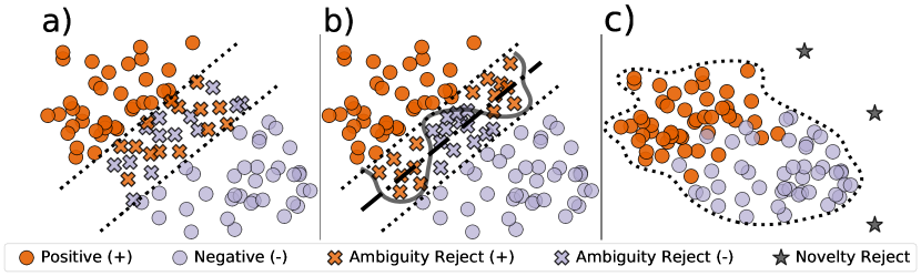
Figure 4: Illustration of a classification scenario where the two classes overlap in a region. The dotted lines represent the rejector, the dash-dotted line the fitted predictor $h$, and the solid line the ground truth relation $f$. a) shows ambiguity rejection due to a non-deterministic relation between $X$ and $Y$, b) introduces ambiguity rejection due to the model bias, and c) illustrates an example of novelty rejection. While in the first two plots the rejection region is inside the two dotted lines (examples with cross marks are rejected), in the third figure the rejected novel examples (stars) are outside the dotted line.

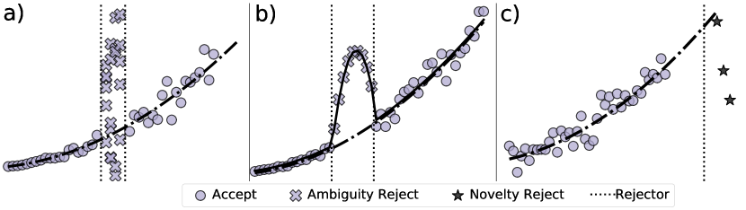
Figure 5: Illustration of a regression scenario where rejection can be applied. The dash-dotted line represents the predictor $h$, while the solid line indicates the true function $f$. In a), examples in between the dotted lines are rejected (cross mark) due to the high variance of $Y$. In b), examples indicated with the cross mark are rejected due to the incorrect model bias. In c), star-marked examples are rejected because they differ from the training data (novelties).

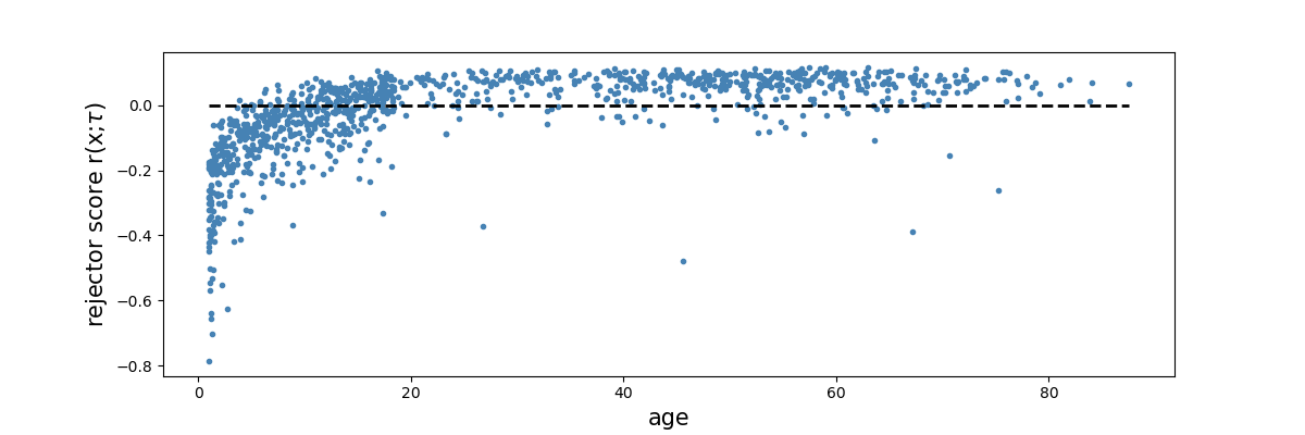
Figure 6: Results of a novelty reject option in a sleep stage scoring application (Van der Plas et al.,, 2021). The predictor is trained only on adults. The accuracy on children ($66.8\%$) is much lower than the accuracy on adults ($77.7\%$). Introducing the reject option mitigates the risk of making incorrect predictions as it ends up rejecting the predictions for most children.

3 Evaluating models with rejection

		Rejection
Prediction		No	Yes
	Correct	True accept (TA)	False reject (FR)
	Incorrect	False accept (FA)	True reject (TR)

Table 1: Confusion matrix for learning-to-reject models. The columns show whether an example is rejected, the rows show whether $h$’s prediction is correct.

Conceptually, a model with a reject option involves evaluating the outputs of both the predictor and the rejector. Thus, its performance can be viewed through the prism of the confusion matrix shown in Table 1, where the columns represent the rejector’s decision and the rows whether the predictor’s output is correct or not. Intuitively, the learning-to-reject model is “correct” if a correct prediction is returned to the user (a true accept) or an example is rejected when the model’s prediction was wrong (a true reject). It is considered to have made a “mistake” if the model provides the user with an incorrect prediction (false accept) or rejects an example for which the model’s prediction was correct.

Viewed through this lens, a model with rejection has two goals. On the one hand, it wants to have high accuracy $\mathcal{A}$ on examples for which it makes a prediction:

$$\mathcal{A} = \frac{TA}{TA+FA}.$$

This makes the model reliable as practitioners can trust its outputs. On the other hand, it wants to have high coverage:

$$\phi = \frac{TA+FA}{TA+FA+FR+TR}.$$

That is, it should make a prediction for as many test examples as possible (De Stefano et al.,, 2000; El-Yaniv and Wiener,, 2010; Lei,, 2014). This can alternatively be viewed as having a low rejection rate, defined as $1-\phi$. This makes the model useful in practice as its predictions can be utilized for decision-making. Unfortunately, these two goals are competing as the accuracy can be increased by limiting the predictions to the most confident cases, i.e., reducing the coverage (Hansen et al.,, 1997; Homenda et al.,, 2016). As a result, metrics specifically tailored to learning to reject must capture this trade-off (Cordelia et al.,, 1998).

Broadly speaking, three categories of metrics exist that evaluate different aspects of a model with rejection:

Evaluating models for a given rejection rate:

This entails having a fixed rejection rate provided by the user. In this case, one only needs to evaluate performance on the non-rejected examples and it is possible to use the standard evaluations (e.g., accuracy (Golfarelli et al.,, 1997));

Evaluating the overall model performance/rejection trade-off:

One can plot the rejection rate on the x-axis and the predictor’s performance obtained on a representative test set on the y-axis, similar to Receiver Operating Characteristic (ROC) analysis;

Evaluating models through a cost function:

This case only requires knowing the model’s output and the costs for (mis)predictions and rejections.

3.1 Evaluating models with a fixed rejection rate.

Given a dataset and a fixed rejection rate, Condessa et al., (2017) argue that a good evaluation metric should meet four main criteria: given a fixed predictor, such metric should: (p1) depend on the model’s rejection rate; (p2) be able to compare two models with different rejectors for a given rejection rate (and for the same predictor); (p3) be able to compare two models with different rejectors with different rejection rates when one clearly outperforms the other; (p4) reach its maximum value for a perfect rejector (i.e., a rejector that rejects all misclassified examples) and its minimum value for a rejector that rejects all accurate predictions. In addition, Condessa et al., (2017) propose three types of evaluation metrics that meet the required conditions:

1. Prediction quality. The model’s prediction quality (PQ) measures the predictor’s performance on the non-rejected examples. For instance, one can use classical evaluation metrics on the accepted examples such as the accuracy

   $$PQ_{\textsc{acc}} = \frac{TA}{TA+FA},$$

   the F-scores (Pillai et al.,, 2011; Mesquita et al.,, 2016) or any other evaluation metric, including fairness metrics (Madras et al.,, 2018). While this allows comparing models with different rejectors, looking only at the prediction quality will tend to favor the model with the highest rejection rate. By being more conservative (i.e., having a lower coverage), the model tends only to offer predictions for the subset of examples for which it is most confident.

2. Rejection quality. The rejection quality (RQ) indicates the rejector’s ability to reject misclassified examples. One way to do this is by comparing the ratio of misclassified examples on the rejected subset ($\frac{TR}{FR}$) to the ratio on the complete dataset ($\frac{FA+TR}{TA+FR}$), i.e.

   $$RQ_{\textsc{ratio}} = \frac{TR}{FR}\Big{/}\frac{FA+TR}{TA+FR}.$$

   Looking only at the rejection quality will favor models with the lowest rejection rate. The lower the rejection rate is, the more likely the rejector is to abstain only on those few examples for which it is most confident that the predictor will make a mistake.

3. Combined quality. The combined quality (CQ) evaluates the model with a reject option as a whole. One way to accomplish this is by combining the predictor’s performance on the non-rejected examples (prediction quality) with the rejector’s performance on the misclassified examples (rejection quality). For instance, using $PQ_{\textsc{acc}}$ and $RQ_{\textsc{ratio}}$ yields to

   $$CQ_{\textsc{acc-ratio}} = \frac{TA+TR}{TA+FA+FR+TR}.$$

   Overall, the combined quality offers a more holistic assessment of the model’s overall performance as it measures both the predictor’s and the rejector’s quality (Lin et al.,, 2018). The downside is that aggregating the two metrics yields a less fine-grained characterization of the model performance. Specifically, in case a model has low CQ, it is hard to ascertain which component, the predictor or rejector, is contributing the most to the model’s poor performance.

Pros and Cons.

The main advantage of this category is that the metrics clearly measure the fine-grained model performance in the given setting. However, using one of these types of metrics may be limiting in some cases. For instance, theoretical research may not care about evaluating the model with rejection for a specific rejection rate, as it is usually specified based on domain knowledge. Moreover, given a rejection rate, not all performance metrics can be always used, as some may suffer from task-related issues. For instance, rejecting a whole class would not allow utilizing metrics like F1-score and AUC for the prediction quality as they need both classes’ labels.

3.2 Evaluating the model performance/rejection trade-off.

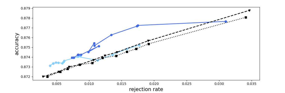
Figure 7: Example of an accuracy-reject curve in which Van der Plas et al., (2023) compare two of their proposed models with a reject option (blue) with two models that were used as baseline (black). The proposed models outperform the baselines but the light blue model only does for rejection rates lower than $0.01$.

To assess the performance-rejection trade-off, a common approach is to evaluate the prediction quality (for non-rejected examples) by varying the rejection rate from $0\%$ to $100\%$, which is known as the Accuracy-Reject Curve (ARC) (Nadeem et al.,, 2010). This involves plotting the rejection rate on the x-axis and the prediction quality (e.g., accuracy) on the y-axis (Hanczar and Sebag,, 2014). Higher curves indicate better performance. Alternatively, risk-based metrics like mean squared error can be plotted, with lower curves indicating better performance (Sambu Seo et al.,, 2000). Sometimes the predictor’s performance on the rejected examples is also shown with the intuition that it should be worse on this subset of the data than on the accepted ones (Zou et al.,, 2011; Condessa et al., 2015c, ; Condessa et al., 2015b, ).

When comparing two models using the ARC method, two scenarios arise. First, one model clearly outperforms the other in terms of prediction quality for all rejection rates. Second, the models show varying prediction quality across different rejection rates. To illustrate this, consider Figure 7 where the light blue curve only outperforms the black curves if the rejection rate is lower than $0.01$. When it is not clear which model performs best, the overall performance can be assessed using the Area Under the ARC Curve (AURC), similar to the AUC in standard machine learning (Vanderlooy et al., 2006a, ; Vanderlooy et al., 2006b, ; Landgrebe et al.,, 2006). In this example, the AURC of the light blue curve will be higher than the AURC of the black curves, indicating that it performs better overall than the black curves.

Pros and Cons.

The main advantage of this category is that any prediction quality metric can be used on the y-axis. Moreover, they provide a high-level overview of how the model works for different rejection rates. However, generating these curves can be challenging for two reasons. First, some rejectors do not allow directly setting the rejection rate (Wu et al.,, 2007; Homenda et al.,, 2014), but they might have other hyperparameters (e.g., rejection threshold). Mapping these to rejection rates may be challenging and may not be possible to achieve all possible rejection rates. Second, altering the rejection rate of a model with rejection can require completely retraining the whole model. This may be too computationally demanding to perform a fine-grained analysis (Condessa et al.,, 2017).

3.3 Evaluating models through a cost function.

For classification tasks, one can ask the user to specify the costs for (mis)predictions as well as for rejection and evaluate a model by its (expected) total cost at test time. Although the costs can be designed as a continuous function of the examples (Mozannar and Sontag,, 2020; De et al.,, 2021), the cost function typically accounts only for three constant costs: the cost of correct prediction $C_{c}$, the cost of a prediction error $C_{e}$, and the cost of rejection $C_{r}$ such that $C_{c}<C_{r}<C_{e}$ (De Stefano et al.,, 2000; Balsubramani,, 2016; Condessa et al.,, 2013). Without loss on generality, usually one assumes that $C_{c}=0$ and $C_{e}=1$, and normalizes $C_{r}$ consequently by $C_{r}=\frac{C_{r}-C_{c}}{C_{e}-C_{c}}$. Although the costs need to be set based on some domain knowledge, there are two constraints for setting the rejection cost properly. First, it must be lower than a random predictor’s average cost for a classification task with $K$ classes, i.e. $C_{r}\leq\frac{1}{K}$ (Cordella et al., 1995b, ; Herbei and Wegkamp,, 2006). Otherwise, the expected cost of always making a random prediction would be lower than the rejection cost, which nullifies the task of rejection. Second, one should account for possible imbalance classes by setting $C_{r}\leq 1-\max_{k\leq K}P(Y=k)$, where $P(Y=k)$ is the class frequency (Perini et al.,, 2023). In fact, for higher $C_{r}$, a naive model that always predicts the most frequent class $\bar{k}$ would obtain a cost equal to $1-P(Y=\bar{k})$ and rejecting examples would not be worth it for higher rejection costs.

Pros and Cons.

The main benefit of this category is its high interpretability: given a final cost, we can easily go back to the causes that yield such a cost. Moreover, one can use the same cost function to optimize the model parameters during the learning phase. This ensures coherence between learning the optimal model at training time and measuring its performance at test time. However, this category has the key drawback that the user must set the cost function based on domain knowledge, which is not always easy to obtain. Setting different costs changes the quality of the models, which may end up ranking several compared models differently. A way to alleviate this would be to make the Cost-Reject plot (Hanczar,, 2019), where, similar to the ARC, the x-axis and y-axis represent respectively the normalized rejection cost and the normalized prediction cost (Friedel et al.,, 2006; Abbas et al.,, 2019).

4 Separated rejector

Separated rejectors operate by filtering out unlikely examples. They are typically used for novelty rejection though there are some examples of using them for ambiguity rejection (Asif and Minhas,, 2020). Because the rejector does not use the predictor’s output in any way, it is typically a function of the examples: $r\colon\mathcal{X}\to\mathbb{R}$. Formally, the separated architecture yields the following model:

$$m(x)=\begin{cases}\text{\textregistered}&\text{if }r(x)<\tau\\ h(x)&\text{otherwise.}\end{cases}$$ (4)

If the rejector $r$ outputs a value less than $\tau$, then the model $m$ rejects the example (®). Otherwise, $m$ uses the predictor $h$ to make a prediction.

The separation between predictor and rejector means that the rejector is learned independently of the predictor. The learning task involves learning the rejector itself as well as setting the threshold $\tau$. To align with its goal of identifying unlikely or unexpected examples, a common choice is to use anomaly/outlier, out-of-distribution, or novelty detection algorithms. Three categories of methods can be used for this goal: models that 1) estimate $p(X)$, 2) are one-class classifiers, and 3) quantify the degree of novelty using a data-driven score function.

Learning a separated rejector.

A first option to learn a separated rejector is to use a probabilistic model that estimates the marginal density $p(X)$ and to reject a test example $x$ if $p(x)<\tau$. These probabilistic models often make assumptions about the distribution of the examples and are trained to maximize the likelihood of the training dataset (Vasconcelos et al.,, 1993). For instance, Landgrebe et al., (2004) proposes a locally normal distribution assumption and uses a Gaussian Mixture Model (GMM) to estimate $p(X)$ with a specified number of components whereas others have considered Variational Autoencoders (Wang and Yiu,, 2020) and Normalizing Flows (Nalisnick et al.,, 2019).

Another option to learn a separated rejector is by employing a one-class classification model. Generally, they enclose the dataset into a specific surface and flag any example that falls outside such region as novelty. For instance, a typical approach is to use a One-Class Support Vector Machine (OCSVM) to encapsulate the training data through a hypersphere (Coenen et al.,, 2020; Homenda et al.,, 2014). By adjusting the size of the hypersphere, the proportion of non-rejected examples can be increased (Wu et al.,, 2007).

Alternatively, some models assign scores that represent the degree of novelty of each example (i.e., the higher the more novel), such as $LOF$ (Van der Plas et al.,, 2023) or Neural Networks (Hsu et al.,, 2020). When dealing with these methods, one often initially transforms the scores into novelty probabilities using heuristic functions, such as sigmoid and squashing (Vercruyssen et al.,, 2018), or Gaussian Processes (Martens et al.,, 2023). Then, the rejection threshold can be set to reject examples with high novelty probability.

Learning the rejection threshold $\tau$.

The rejection threshold $\tau$ is a crucial parameter that determines whether an example is rejected or not. In many cases, the threshold is set based on domain knowledge. For instance, one can introduce adversarial examples and set a threshold to reject them all (Hosseini et al.,, 2017). In case the number of novelties is unknown, one can use existing methods to estimate the contamination factor, i.e. the proportion of novelties, and set the threshold accordingly (Perini et al., 2022b, ; Perini et al., 2022a, ). Otherwise, heuristics can be employed, such as rejecting examples falling within the first or second percentiles of correctly classified training examples (Wang and Yiu,, 2020).

Benefits and drawbacks of a separated rejector.

Using a separated rejector has several benefits. First, the rejector is predictor agnostic. Hence, it can be combined with any type of predictor. Second, because the rejector can be trained independently of the predictor, it is possible to augment an existing predictor with a reject option using this architecture. Third, by serving as a filter, the predictor makes fewer predictions. This is particularly advantageous when there is a high computational cost associated with using the predictor. Finally, this architecture is generally simpler to operationalize compared to rejectors that interact with the predictor. However, there are two evident drawbacks. First, not sharing information between the predictor and the rejector results often in sub-optimal rejection performance (Homenda et al.,, 2014). Second, this architecture is typically only used for novelty rejection because it is naturally related to assessing whether $x$ is rare or not while ambiguity rejection requires information on $p(Y|X)$, which is often estimated through the predictor’s output.

5 Dependent rejector

Dependent rejectors analyze the predictor’s output to identify examples that the predictor is likely to mispredict. The rejector is typically represented as a confidence function $c_{h}\colon\mathcal{X}\to[0,1]$ that measures how likely the predictor is to make a correct prediction. Formally, the model for a dependent architecture has the form:

$$m(x)=\begin{cases}\text{\textregistered}&\text{if }r(x;h)<\tau;\\ h(x)&\text{otherwise.}\end{cases}$$ (5)

where $r$ may depend on the feature vector $x$, and on the predictor $h$ through the confidence function $c_{h}$. Similar to the separated rejector, the model rejects the example (®) only if the rejector outputs a value lower than $\tau$. Without loss of generality, we assume the confidence values $c_{h}(x)\in[0,1]$, as one can always transform a score function into this range.

The learning task for a dependent rejector usually entails (1) selecting a confidence function that measures how confident the predictor is in its predictions, and (2) setting the rejection threshold $\tau$.

Learning a dependent rejector: types of confidence function $c_{h}$.

The form of the confidence function depends on the desired rejection type. For ambiguity rejection, the metric should indicate the variability of the target variable or the potential predictor bias. For novelty rejection, the confidence should capture the example’s similarity to the training data. We distinguish among four ways to derive the confidence scores: i) estimating the conditional probability $P(Y|X)$, ii) estimating the class conditional density $p(X|Y)$, iii) performing a sensitivity analysis, and iv) exploiting the predictor’s properties.

The conditional probability approaches allow for ambiguity rejections by using the maximum of the class conditional probability as confidence function (Pazzani et al.,, 1994; Fumera et al.,, 2004; Lam and Suen,, 1995)

$$c_{h}(x) = \max_{k\in\mathcal{Y}}P(Y=k|X=x)$$ (6)

where $k$ is either the true target value or the predictor’s output. Low $P(Y|X)$ values for two or more targets $k_{1},k_{2}\in\mathcal{Y}$ indicate high randomness of the data or proximity to the decision boundary (Arlandis et al.,, 2002). Deriving the conditional probabilities from the predictor’s outputs can be done by post-processing the predictor’s output using techniques such as sigmoid calibration for binary classification tasks (Cordella et al.,, 2014; Brinkrolf and Hammer,, 2017)

$$P(Y=1|X=x) \approx \frac{1}{1+\exp(Ah(x)+B)},$$

with parameters $A$ and $B$ learned during the training (Brinkrolf and Hammer,, 2018), softmax transformation for multi-class classification tasks (Kwok,, 1999)

$$P(Y=k|X=x) \approx \frac{\exp{(h_{k}(x))}}{\sum_{j\in\mathcal{Y}}\exp{(h_{j}(x))}},$$

where $h_{j}(x)$ is the predictor’s output for $x$ related to class $j$, or by fitting Gaussian Processes for regression tasks (Sambu Seo et al.,, 2000). In case of multiple predictors $h_{1},\dots,h_{V}$, one can also measure the ensemble agreement as the conditional probability (Glodek et al.,, 2012; Zhang,, 2013)

$$P(Y=k|X=x) \approx \frac{\sum_{v=1}^{V}\mathbbm{1}[h_{v}(x)=k]}{V}.$$

On the other hand, the class conditional density approaches perform novelty rejection putting (Dubuisson and Masson,, 1993; Dübuisson et al.,, 1985)

$$c_{h}(x) = \max_{k\in\mathcal{Y}}p(X=x|Y=k).$$ (7)

Intuitively, a low density $p(X|Y)$ expresses that a sample is rare (Condessa et al., 2015b, ). Common methods to estimate the confidence in Eq. 7 employ generative predictors that directly measure the data density such as Gaussian Mixture Models (GMMs) (Vailaya and Jain,, 2000). It is also possible to employ heuristic approaches such as normalizing the class distance between the example $x$ and its $v-$th nearest neighbor $x^{\prime}$ (Conte et al.,, 2012; Villmann et al.,, 2015; Fischer et al., 2014b, ), i.e.

$$p(X=x|Y=k) \approx \frac{d(x,x^{\prime})}{\sum_{\{(x_{*},y_{*})\in D\colon y_{*}=k\}}d(x_{*},x^{\prime}_{*})}$$

and computing the proportion of neighbors within a specified radius $R$ (Berlemont et al.,, 2015) as

$$p(X=x|Y=k) \approx \frac{|\{x^{\prime}\colon d(x,x^{\prime})\leq R,(x^{\prime},y^{\prime})\in D,y^{\prime}=k\}|}{\sum_{(x^{\prime},y^{\prime})\in D}|\{x_{*}\colon d(x^{\prime},x_{*})\leq R,(x_{*},y_{*})\in D,y_{*}=k\}|}.$$

The sensitivity analysis line allows only ambiguity rejection, as it measures the robustness of the predictor under perturbation of either (a) its parameters or (b) the examples (Lewicke et al.,, 2008; Hellman,, 1970). Intuitively, slightly perturbing the predictor’s parameters has major effects on the predictions only for examples that fall in the proximity of the decision boundary: slight variations of the parameters yield slight changes in the decision boundary, which, in turn, may end up flipping the predictions for some examples. Examples of employed perturbations involve adding some noise to the model’s parameter values (e.g., adding a random sample from a normal distribution with null mean and small variance to the weights of a neural network), employing neural networks with a dropout layer (Geifman and El-Yaniv,, 2017), or using a Bayesian simulation (Perini et al., 2020b, ). In the case of constructing multiple predictors, a common and simple confidence metric is

$$c_{\{h_{1},\dots,h_{M}\}}(x)=1-\mathrm{Var}\{h_{1}(x),\dots,h_{M}(x)\}$$

where $h_{1},\dots,h_{M}$ are the $M$ predictors constructed by perturbing the parameters, and the variance is scaled to be in $[0,1]$. In some cases, one can directly employ an ensemble of $M$ similar predictors and measure the variance of their predictions (Fumera and Roli,, 2004; Jiang et al.,, 2020).

Alternatively, one can perturb the test example $x$ to be $x+\varepsilon$, where $\varepsilon$ is a random noise such that $\|\varepsilon\|$ is small. Intuitively, we want a predictor’s output to remain the same when the example is only slightly perturbed. Thus, the confidence metric should reflect the robustness of $h$ (Mena et al.,, 2020; Denis and Hebiri,, 2020; Joana et al.,, 2021), such as

$$c_{h}(x)=P(h(x+\varepsilon)=h(x)),$$

which measures how likely it is that the prediction does not change when the example is perturbed. More generally, we can apply transformations such as rotations and symmetries to the examples (Chen et al.,, 2018). Finally, because choosing a specific value for $\varepsilon$ is hard, one can use existing approaches to find each example’s minimum $\varepsilon$ that will alter its predicted label (Devos et al.,, 2021) and derive a confidence metric as a function of the training $\varepsilon$.

The property-based methods consist of learning the confidence based on some of the predictor’s properties, such as using the leaf configurations of a tree ensemble or the neural network’s weight of specific neurons. This line allows both ambiguity and novelty rejection, depending on the utilized property. These methods tend to exploit heuristic and data-driven intuitions and there are no overarching themes that connect these intuitions. For instance, Devos et al., (2023) present a method to detect evasion attacks in tree ensembles. By enumerating the leaves of each tree as $o_{i}$, they map each example $x$ to the configuration $o=(o_{1},\dots,o_{V})\in\mathbb{N}^{V}$ of the $V$ activated leaves (one per tree) when passing $x$ as input to the ensemble. In such output configuration space, they quantify the proximity to the decision boundary by measuring the Hamming distance between the configuration $o$ of a test example with ensemble’s prediction $y$ and the closest training example’s configuration $o^{\prime}$ with flipped prediction $\hat{y}\neq y$:

$$\textsc{OC-score}(x)=\min_{o^{\prime}\in R_{\hat{y}}}\left(\sum_{v=1}^{V}\mathbbm{1}\left[o_{v}\neq o^{\prime}_{v}\right]\right)$$

where $R_{\hat{y}}$ is the set of training configurations with flipped predictions. One can derive a confidence metric $c_{h}$ by, for instance, min-max normalizing the OC-score. On the other hand, confidence values can also be derived from the weight vectors of a Self-Organizing Map (SOM) (Gamelas Sousa et al., 2014b, ; Gamelas Sousa et al.,, 2015). Because SOM ’s can approximate the input data density, they approximate $p(X=x|Y=k)$ with $p(w|Y=k,X=x)$, where $w$ are the weights of the neural network, using standard statistical techniques, such as the Parzen Windows (Alhoniemi et al.,, 1999). Moreover, El-Yaniv and Wiener, (2011) propose a disbelief principle, which computes the confidence function by measuring how much the predictor $h$ deteriorates if retrained with the constraint to predict a specific example $x$ differently (i.e., $h_{x}$)

$$c_{h}(x)=\frac{1}{R(h_{x})-R(h)},$$

where $R(h_{x})>R(h)>0$. Finally, the literature presents additional ad-hoc confidence metrics for $k$-NN and Random Forest (Göpfert et al.,, 2018; Dalitz,, 2009).

Learning the rejection threshold $\tau$.

Setting an appropriate rejection threshold $\tau$ is crucial for having an accurate dependent rejector. At a high level, the threshold is set in three main ways: using domain knowledge, adhering to user-provided constraints, or tuning it empirically based on some objective function.

In some situations, users possess domain knowledge that enables setting $\tau$ to achieve a desired rejection rate $\rho$ (Le Capitaine and Frélicot,, 2012; Pang et al.,, 2021). Setting $\tau$ in this situation entails (1) ranking training examples based on their confidence level, and (2) setting $\tau$ such that the desired percentage of predictions are rejected (Sotgiu et al.,, 2020), that is, at

$$P_{X}(c_{h}(x)<\tau)=\rho.$$

Note that this approach is also used when evaluating the model performance/rejection trade-off, which needs to measure the model performance for a fixed rejection rate (see Sec. 3.2) (Ma et al.,, 2001; Heo et al.,, 2018; Fumera et al.,, 2003).

In other cases, users provide knowledge as specific constraints that should be satisfied (Pietraszek,, 2005). On the one hand, the user may provide an upper bound $\mathfrak{R}$ for the rejection rate and aim to limit the number of rejections. This results in learning the appropriate $\tau$ by minimizing the model misclassification risk while adhering to the rejection rate constraint (Zhou et al.,, 2022; Pugnana and Ruggieri,, 2022, 2023)

$$\tau=\operatorname*{arg\,min}_{t\in[0,1]}P_{XY}(h(x)\neq y,c_{h}(x)\geq t)\quad\text{ subject to }\quad P_{X}(c_{h}(x)<t)\leq\mathfrak{R}.$$

On the other hand, the user may provide an upper bound $\mathfrak{M}$ for the proportion of mispredictions, and aim to control the allowable error (Varshney,, 2011; Sayedi et al.,, 2010). Thus, one needs to learn $\tau$ by setting up the complementary problem as before, namely by minimizing the model rejection rate while satisfying the constraints on error (Li and Sethi,, 2006; Franc and Prusa,, 2019; Franc et al.,, 2021)

$$\tau=\operatorname*{arg\,min}_{t\in[0,1]}P_{X}(c_{h}(x)<t)\quad\text{ subject to }\quad P_{XY}(h(x)\neq y,c_{h}(x)\geq t)\leq\mathfrak{M}.$$

Moreover, one can generalize this problem by finding the threshold $\tau$ such that the predictor’s misclassification risk at test time is guaranteed to be bounded with high probability (Geifman and El-Yaniv,, 2017).

Finally, it is possible to set $\tau$ empirically according to some objective function. The most common approach is to set a single global threshold $\tau$, which makes the rejection both simple and transparent, yet usually effective (Fukunaga and Kessell,, 1972). This is the case for Chow’s rule (Chow,, 1970) which involves learning the optimal $\tau$ by minimizing the risk function that includes the expected error rate and the rejection rate

$$\tau=\operatorname*{arg\,min}_{t\in[0,1]}\left[{\underbrace{\int_{\{x\in\mathcal{X}\colon c_{h}(x)\geq t\}}(1-c_{h}(x))\,p(x)\,dx}_{\textsc{Error rate}}}+t{\underbrace{\int_{\{x\in\mathcal{X}\colon c_{h}(x)<t\}}p(x)\,dx}_{\textsc{Rejection rate}}}\right].$$ (8)

However, in real-world scenarios, obtaining complete knowledge of class distributions is challenging, limiting the applicability of Chow’s rule (Shekhar et al.,, 2019). Thus, in a binary classification case, Tortorella, (2000) proposes to use two rejection thresholds $\tau_{1}$ and $\tau_{2}$ such that

$$h(x)=\begin{cases}0&\text{if }c_{h}(x)<\tau_{1};\\ 1&\text{if }c_{h}(x)>\tau_{2};\\ \text{\textregistered}&\text{if }\tau_{1}\leq c_{h}(x)\leq\tau_{2}\end{cases}$$ (9)

with $c_{h}(x)=P(Y=1|X=x)$. He proposes to learn $\tau_{1}$, $\tau_{2}$ by optimizing a cost function that is identical to finding the intersection between the cost function and the convex hull of the ROC curve

$$\tau_{1} = \operatorname*{arg\,max}_{t\in[0,1]}P(Y=1)(C_{fn}-C_{r})FNR(t)+P(Y=0)(C_{tn}-C_{r})TNR(t)$$ (10)

$$\tau_{2} = \operatorname*{arg\,max}_{t\in[0,1]}P(Y=1)(C_{tp}-C_{r})TPR(t)+P(Y=0)(C_{fp}-C_{r})FPR(t)$$ (11)

where $C_{fn}$, $C_{fp}$, $C_{tn}$, and $C_{tp}$ are the costs for false negatives, false positives, true negatives, and true positives, while $FNR(t)$, $TNR(t)$, $TPR(t)$ and $FPR(t)$ are the false negative, false positive, true negative and true positive rates obtained by evaluating the models with the thresholds set to $t$. This approach is theoretically equivalent to Chow’s rule under the Bayesian optimality assumption (Santos-Pereira and Pires,, 2005; Du et al.,, 2010). However, when estimating posterior probabilities, Chow’s rule is not suitable, and $\tau$ should be learned using a cost-based approach (Marrocco et al.,, 2007; Kotropoulos and Arce,, 2009). Different approaches have extended Tortorella,’s method to address other scenarios (Sansone et al.,, 2001), such as stable formulations of ROC curves for small datasets (Jigang et al.,, 2006), robust and fast-to-retrain rejections for cost-sensitive situations (Dubos et al.,, 2016; Fischer et al., 2015b, ), and tailored solutions for learning meta-classifiers or handling multiple classes (Pietraszek,, 2007; Cecotti and Vajda,, 2013).

For tasks requiring a more fine-grained rejection capability, considering multiple local thresholds $\tau_{1},\tau_{2},\ldots$ (up to a finite number) may be beneficial (Muzzolini et al.,, 1998; Kummert et al.,, 2016; Krawczyk and Cano,, 2018). Normally, setting local thresholds requires dividing the feature space into $J$ regions $\mathcal{J}_{i}$ and setting a (local) threshold in each region. For instance, one can design regions and thresholds by

• constructing one region for each class, i.e. $\mathcal{J}_{i}=\{x_{*}\ |\ y_{*}=i\}$, which means that the number of regions $J$ equals the number of classes $K$ (Fumera et al.,, 2000); then, one often finds the local threshold by using for each $\mathcal{J}_{i}$ the same approach as for global thresholds;

• using the Voronoi-cell decomposition, which requires $J$ prototypes $w_{i}$ to have $\mathcal{J}_{i}=\{x_{*}\ |\ d(x_{*},w_{j})\leq d(x_{*},w_{k})\ \forall k\neq i\}$, for $i\leq J$ (Villmann et al.,, 2015; Fischer et al., 2015a, ; Fischer et al., 2015b, ; Fischer and Villmann,, 2016); then, Fischer et al., 2014a present a greedy optimization method to adaptively determine local thresholds using a heuristic principle;

• setting up an optimization problem that finds the optimal thresholds by assigning different class rejection costs; for instance, in binary classification, Zheng et al., (2011) proposes to find

  $$\begin{split}\tau_{1},\tau_{2}=\operatorname*{arg\,min}_{0\leq t_{1},t_{2}\leq 1}\Big{[}&P_{XY}(c_{h}(x)<t_{1}|y=0)C_{r,0}+P_{XY}(c_{h}(x)<t_{2}|y=1)C_{r,1}\\ &+P_{XY}(m(x)\neq y)C_{e}\Big{]}\end{split}$$

  where $C_{r,0}$ and $C_{r,1}$ are the costs for rejecting examples from the negative and positive classes;

• optimizing an objective function that accounts for different user-specified class misclassification risks $\mathfrak{M}_{1},\dots,\mathfrak{M}_{K}$; Lin et al., (2022) treat each class independently, setting

  $$L(t_{k})=\hat{A}(t_{k})+\sum_{j}^{K}\lambda_{j}(\hat{\mathfrak{M}}_{j}-\mathfrak{M}_{j})^{2}$$

  where $\hat{A}(t_{k})$ is any ambiguity metric, $\lambda_{j}$ is a penalization term that needs to be set to high values to penalize high differences between the model’s misclassification risk $\hat{\mathfrak{M}}$ and the user-specified target.

Although multiple thresholds give more fine-grained control over a rejector’s performance (Laroui et al.,, 2021; Gangrade et al., 2021a, ), this is usually more computationally expensive. However, Fischer et al., (2016) propose efficient schemes for optimizing local thresholds and show that the computation time can be reduced to polynomial (Boulegane et al.,, 2019).

Benefits and drawbacks of a dependent rejector.

Designing a dependent rejector has several benefits. First, the interaction between the predictor and rejector enables both types of rejection, because the rejector learns from the predictor’s output the regions of the feature space where examples are mispredicted or unlikely to fall. Second, a dependent rejector can extend an existing predictor (including black-box) by simply setting a proper threshold on a confidence measure. Third, it allows the reuse of previously learned models, eliminating the need for costly retraining (Zou et al.,, 2011; Tang and Sazonov,, 2014). Fourth, a confidence-based rejection could be improved by considering multiple confidence metrics where each one captures different aspects of the underlying uncertainty (Tax and Duin,, 2008). However, this architecture has potential drawbacks as well. First, the quality of the dependent rejector is highly influenced by the quality of the confidence metric, which is usually hard to evaluate. Second, typically a dependent rejector does not affect the predictor’s learning phase. This results in possible sub-optimal predictions of the model with a reject option.

6 Integrated rejector

The integrated rejector combines the rejector and predictor into a single model where it is impossible to distinguish between the role of the $h$ and the $r$. Formally, the model with integrated reject option acts as

$$m(x)\in\mathcal{Y}\cup\{\text{\textregistered}\}.$$ (12)

Conceptually, this model simply includes ® as an additional output.

This architecture usually needs a unique algorithm for learning predictor and rejector in tandem (Cortes et al., 2016a, ; Cortes et al., 2016b, ). There are two distinct approaches to learning an integrated rejector. The first approach is model-agnostic and involves designing an objective function that penalizes (mis)predictions as well as rejections. The second approach is model-specific and entails integrating a rejector into an existing predictor, where rejection becomes part of the decision-making process.

Learning a model-agnostic integrated rejector.

Typically, learning a model that simultaneously makes accurate predictions and rejects the examples that will be otherwise mispredicted can be done by simply designing a specialized objective function (Mozannar and Sontag,, 2020). Then, such a function can be minimized using potentially any existing optimizer, which makes it model-agnostic. For instance, a simple cost-based objective for any hypothesis $m$ can be expressed as

$$L=\mathbb{E}_{p(X,Y)}\left[C_{c}\mathbbm{1}_{m(x)=y}(x)+C_{r}\mathbbm{1}_{m(x)=\text{\textregistered}}(x)+C_{e}\mathbbm{1}_{m(x)\neq\{y,\text{\textregistered}\}}(x)\right].$$

For tasks other than classification, ad-hoc loss functions are used, such as those for multilabel classification (Pillai et al.,, 2013; Nguyen and Hüllermeier,, 2020, 2021), regression (Asif and Minhas,, 2020; Kalai and Kanade,, 2021), online learning (Cortes et al.,, 2018; Kocak et al.,, 2020), and multi-instance learning (Zhang and Metaxas,, 2006). However, in many cases, surrogate losses are employed to enable efficient optimization, as learning from discrete losses is computationally impractical (Wegkamp,, 2007; Grandvalet et al.,, 2009; Cao et al.,, 2022). Consequently, the original loss $L$ is converted into a convex loss by utilizing surrogate functions $\psi\colon\mathbb{R}\to\mathbb{R}$, such as the logistic and hinge functions (Ramaswamy et al.,, 2018; Zhang et al.,, 2018; Bartlett and Wegkamp,, 2008):

$$\text{Logistic: }\psi(L)=\frac{1}{1+\exp(L)},\qquad\text{Hinge: }\psi(L)=\begin{cases}1-\frac{1-C_{r}}{C_{r}}L&\text{ if }L<0\\ 1-L&\text{ if }0\leq L<1\\ 0&\text{ otherwise}\end{cases}$$

Numerous studies in the literature have explored the properties of surrogate loss functions (Yuan and Wegkamp,, 2010), including calibration effects (Ni et al.,, 2019; Charoenphakdee et al.,, 2021), estimates of bounds for misclassification risk (Shekhar et al.,, 2019; Kato et al.,, 2020), penalization effects in high-dimensional spaces (Wegkamp and Yuan,, 2012), proximity to the optimal Bayes solution (Bounsiar et al.,, 2008; Shen et al., 2020a, ), and convergence rate analysis (Denis and Hebiri,, 2020).

Lastly, one can allocate an extra class $K+1$ (commonly known as the reject class) for rejection and assign a specific penalization cost $C_{r}$ for predicting such a class. With this setting, there are two main alternatives. In the first case, there are no actual examples belonging to this class. Thus, these approaches design loss functions to enable the classifier to assign on its own a positive score to ambiguous examples (Huang et al.,, 2020; Feng et al.,, 2022). For instance, Ziyin et al., (2019) propose the loss function

$$L=\mathbb{E}_{p(X,Y)}\left[\log(s_{k}(x)+\frac{1}{C_{r}}s_{K+1}(x))\right],$$

where $s_{k}(x)$ and $s_{K+1}(x)$ are probabilities, respectively, for the class $y=k$ and $K+1$ (rejection). At a high level, decreasing the rejection cost $C_{r}$ results in higher chances of rejection. In the second case, one artificially generates examples ${x_{n+1},\dots,x_{N}}$ (e.g., adversarial examples) and assigns them to the rejection class $K+1$. By training a predictor with $K+1$ classes, the reject option is naturally incorporated as output, and any (multi-class) predictor can be used for novelty (Vasconcelos et al.,, 1995; Singh and Markou,, 2004; Urahama and Furukawa,, 1995) or ambiguity rejection (Thulasidasan et al.,, 2019; Pang et al.,, 2022).

Learning a model-specific integrated rejector.

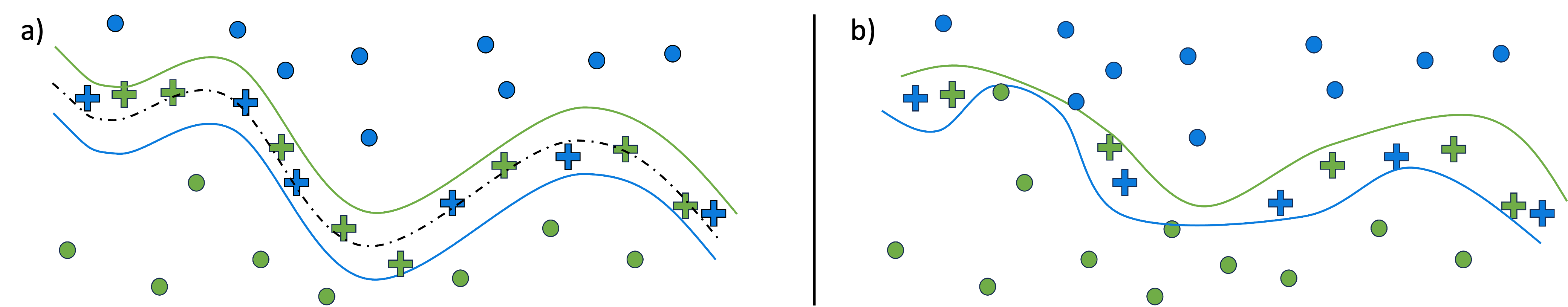
Figure 8: Two cases of Integrated SVMs: (a) on the left side, the two hyperplanes are parallel and equidistant to the decision boundary (dashed line); (b) on the right side, each SVM gives higher priority to one class by limiting mispredictions.

In many practical use cases, one may already know that a specific class of models works well within the given context, such as SVM models in medical applications (Hanczar and Dougherty,, 2008; Hamid et al.,, 2017). Given a specific predictor, its learning algorithm can be slightly adapted to include the reject option. For instance, integrated SVMs set two (or more) hyperplanes on the feature space and reject all the examples located in between them (Pillai et al.,, 2011; Lin et al.,, 2018; Zidelmal et al.,, 2012). Figure 8 shows two common cases to learn the hyperplanes. First, one can parametrize the hyperplane as $w\cdot x+b\pm\varepsilon=0$, with $\varepsilon\geq 0$, which results in parallel and equidistant hyperplanes from the decision boundary, where $\varepsilon$ indicates the distance (Fumera and Roli,, 2002). Learning such hyperplanes requires minimizing the empirical loss

$$L=\frac{1}{2}w\cdot w+C\sum_{i=1}^{n}l(\xi_{i},\varepsilon)-\sum_{i=1}^{n}\alpha_{i}\left[y_{i}(w\cdot x_{i}+b)-1+\xi_{i}\right]$$

where $w$ is the weight vector, $b$ is the intercept of the hyperplane, $C$ is a (large) hyperparameter that regulates the importance of the performance/rejection trade-off expressed inside the function $l(\xi_{i},\varepsilon)$, and $\alpha_{i}$ are the Lagrangian multipliers. Second, the two hyperplanes can be parametrized as

$$w^{\prime}\cdot x+b^{\prime}=0\quad\text{and}\quad w^{\prime\prime}\cdot x+b^{\prime\prime}=0.$$

By formulating two distinct optimization problems, one can learn the parameters of these hyperplanes. In this approach, one hyperplane is highly penalized for mispredicting the positive class, while the other one is for the negative class. Essentially, this technique yields two SVMs that have few mispredictions on either class, and examples falling in between the hyperplanes can be naturally rejected (Varshney,, 2006). With the same approach, one can also learn a OCSVM for each class to reject test examples that lie outside any learned hypersphere (novelty) or within two overlapping hyperspheres (ambiguity) (Lotte et al.,, 2008; Loeffel et al.,, 2015; Wu et al.,, 2007). Finally, Gamelas Sousa et al., 2014a shows that limiting the number of support vectors reduces the computational cost, while still ensuring high performance in most cases.

However, in several cases, more than two SVMs are used. For instance, in multi-label classification one can exploit as many SVMs as the number of labels and fit each hyperplane to discriminate between one class and all the others (Pillai et al.,, 2011). This raises the issue of defining rejection in the regions of intersection between some, but not all, of the hyperplanes. To address this, a natural solution is to utilize a data-replication method (Gamelas Sousa et al.,, 2009). This approach involves replicating the complete dataset for each class $k\in\mathcal{Y}$, adding a new dimension $z$ with the class number, changing the target variable of each replica to a discrete one-vs-all label, and discriminating class $k$ from the other classes (Cardoso and Pinto Da Costa,, 2007; da Rocha Neto et al.,, 2011).

Finally, Neural Network models allow integrating the rejector and predictor into the same structure by modifying their output layers (Gangrade et al., 2021b, ; Ziyin et al.,, 2019). Geifman and El-Yaniv, (2019) propose to introduce an additional head $m_{r}$ into the network that is dedicated to rejection. Specifically, $m_{r}$ is set as a sigmoid function and used such that

$$m(x)=\text{\textregistered}\quad\text{ if }m_{r}(x)<0.5.$$

Similar to the SVM case, Gasca A. et al., (2011) and Mesquita et al., (2016) measure the disagreement of two Neural Networks trained to prioritize the classes differently. Specifically, they assume a binary classification task and use the output of two neural networks $h_{1}$, $h_{2}$ to predict the positive class if $h_{1}(x),h_{2}(x)\geq 0$, the negative class if $h_{1}(x),h_{2}(x)<0$ and rejection if they disagree on the sign. For this task, they use two weighted Extreme Learning Machines (wELM) (Zong et al.,, 2013), namely two neural networks with $Q$ hidden neurons that output

$$h_{*}(x)=\sum_{q=1}^{Q}w_{y}\beta_{q}g(a_{q}\cdot x+b_{q})$$

where $w_{y}$ is the cost related to the example $x$ that belongs to the class $y$, $a_{q}$ is the weight vector connecting the $q$-th hidden node and the input nodes, $b_{q}$ is the bias of the $q$-th hidden node and $g$ is the activation function. By setting the class misprediction costs, learning the parameters $\beta=(\beta_{1},\dots,\beta_{Q})$ requires using the traditional weighted least square formulation $\min\|H\beta-Y\|^{2}$ so that

$$\beta=(H^{T}WH)^{-1}H^{T}WY$$

where $H$ is the $n\times Q$ matrix of activation functions $h_{iq}=g(a_{q}\cdot x_{i}+b_{q})$, $W$ is the $n\times 1$ matrix of class costs (one per example) and $Y$ is the target vector. Thus, each network limits one class mispredictions and the region of disagreement is designed to be the rejection region.

Benefits and drawbacks of an integrated rejector.

This architecture has two key benefits. First, integrating the predictor and rejector means that both aspects of the model are optimized toward the task at hand. This can improve the performance of the model with rejection when compared to using other architectures because the predictor’s and the rejector’s components can affect each other. Second, because it is a unique model, the bias introduced by the model with rejection is potentially less than in the scenario where the predictor and rejector are two different models. However, this architecture has potential drawbacks, as designing such a rejector might not be trivial. First, it requires extensive knowledge about the predictor in order to integrate the reject option. Second, it may require developing a novel algorithm to learn the model with a reject option from data. Finally, it is computationally more expensive than the other architectures, as any changes to the rejector require retraining the entire model, which can be time-consuming (Clertant et al.,, 2020; Shpakova and Sokolovska,, 2021).

7 Combining multiple rejectors

Most rejectors are tailored towards a single rejection type. However, by combining multiple rejectors one can enable multiple rejections, such as performing both ambiguity and novelty rejection. We distinguish between two types of combinations of rejectors based on whether the rejectors’ rejection regions overlap or not because examples in overlapping regions require deeper analysis (e.g., to specify the underlying rejection type).

First, when rejectors do not overlap (or when we are not interested in the example’s rejection type), one can simply combine the rejection sets by a logical $or$-rule: reject the example if any of the rejectors rejects it and assign such rejection type (Frélicot,, 1997; Suutala et al.,, 2004). For instance, given $\mathcal{Z}$ rejectors $r_{1},r_{2},\dots,r_{\mathcal{Z}}$ with thresholds $\tau_{1},\tau_{2},\dots,\tau_{\mathcal{Z}}$, one can combined them into $m$ as

$$m(x)=\begin{cases}\text{\textregistered}\quad&\text{if }\exists\,i\leq\mathcal{Z}\,\colon r_{i}(x;h)<\tau_{i}\\ h(x)\quad&\text{otherwise}\end{cases}$$

Second, when rejectors overlap in some regions a simple $or$-rule is insufficient, because rejectors may disagree on the type of rejection. Typically, existing works carefully select the order to evaluate the rejectors. This is usually done in a multi-step architecture: either by stacking only the rejectors (Frélicot,, 1998; Frélicot and Mascarilla,, 2002), or even using multiple models with rejection (Pudil et al.,, 1992; Barandas et al.,, 2022). For instance, given $\mathcal{Z}$ rejectors $r_{1},r_{2},\dots,r_{\mathcal{Z}}$ with thresholds $\tau_{1},\tau_{2},\dots,\tau_{\mathcal{Z}}$, one can order rejectors by importance and combine them as

$$m(x)=\begin{cases}\text{\textregistered}_{1}\quad&\text{if }r_{1}(x;h)<\tau_{1};\\ \text{\textregistered}_{2}\quad&\text{if }r_{1}(x;h)\geq\tau_{1}\text{ and }r_{2}(x;h)<\tau_{2};\\ \vdots\\ h(x)\quad&\text{if }r_{i}(x;h)\geq\tau_{i}\ \forall\,i\leq\mathcal{Z};\\ \end{cases}$$

where $\text{\textregistered}_{i}$ indicates the rejector $r_{i}$’s type of rejection.

8 Applications of machine learning models with rejection

In safety-sensitive domains, making the wrong decision can have serious consequences such as fatal accidents with self-driving cars, major breakdowns in industrial settings or incorrect diagnoses in medical applications. In these domains, rejection can be used to make cautious predictions. However, the number of papers discussing machine learning with rejection in practical applications is still limited. In this section, an overview of these papers is given.

Biomedical applications.

Machine learning with rejection is primarily explored in medical applications due to the potential consequences of incorrect decisions (Liu et al.,, 2022). The main focus is on ambiguity rejection for medical diagnosing, specifically the detection and classification of diseases. If the model is confident enough, the detection results are automatically translated into a diagnosis. Otherwise, a medical expert verifies the detection (Kompa et al.,, 2021). For instance, vocal pathologies are detected using voice recording data, where a linear classifier is trained and uncertain predictions are rejected based on a threshold of the derived posterior probability (Kotropoulos and Arce,, 2009). Spine disease diagnosis employs the data-replication method, which predicts only when two biased classifiers agree (Gamelas Sousa et al.,, 2009). Cancer detection, particularly breast tumor detection, benefits from a reject option implemented with an SVM classifier using confidence-based rejection (Guan et al.,, 2020). The rejection thresholds are chosen to limit the rejection rate and reduce manual effort.

Other biomedical applications have also adopted the use of a reject option. Lotte et al., (2008) conduct an experiment on distinguishing hand movements using brain activity. They employ a separate novelty rejector trained in a supervised manner to discard brain activity associated with other activities. Lewicke et al., (2008) explore sleep stage scoring with both types of rejection, utilizing confidence metrics derived from a Neural Network classifier’s neural activities. Another sleep stage scoring application utilizes a separate rejector based on Local Outlier Factor (LOF) anomaly scores for novelty rejection, identifying patients who deviate from the training data (Van der Plas et al.,, 2021). Some papers compare the performance of multiple models with rejection to determine the optimal approach for specific biomedical applications. For instance, Kang et al., (2017) predict the effectiveness of a diabetes drug for individual patients, while Tang and Sazonov, (2014) investigate the classification of body positions using sensors placed in patients’ shoes. Lastly, a medical application focuses on the analysis of tissue examples, aiming to classify each pixel of tissue images into categories such as bone, fat, or muscle (Condessa et al.,, 2013; Condessa et al., 2015a, ).

Engineering applications.

Applications in engineering can also benefit from a reject option. For instance, in the chemical identification of gases, time-series data is processed by two classifiers to classify the observed gas. Classification occurs only when there is agreement between the classifiers, and ambiguous predictions are rejected until consensus is reached (Hatami and Chira,, 2013). A similar ambiguity rejection technique, rejecting when two classifiers disagree, is employed in defect detection in software applications (Mesquita et al.,, 2016). Fault detection in steam generators utilizes a set of one against all SVM classifiers, and rejection is based on the distance to the decision boundary of these classifiers, allowing for both rejection types (Zou et al.,, 2011). Finally, Hendrickx et al., (2022) employs a separated novelty rejector for vehicle usage profiling.

Economics applications.

In the domain of economics, two applications of machine learning with rejection have been proposed, both focused on ambiguity rejection and novelty rejection. The first application uses a Learning Vector Quantization (LVQ) to classify dollar bills by value (Ahmadi et al.,, 2004). Confidence metrics are obtained from the classifier for both types of rejection. The second application investigates a few rejection techniques on top of a predictor to decide whether to grant a loan (Coenen et al.,, 2020)

Image recognition applications.

Reject options are usually available for analyzing text styles and reading handwritten numbers (Fumera and Roli,, 2004), used for both ambiguity rejection (Xu et al.,, 1992; Huang and Suen,, 1995; Rahman and Fairhurst,, 1998) and novelty rejection (Lou et al.,, 1999; Arlandis et al.,, 2002). These methods employ a confidence-based dependent rejector. Additionally, there is a paper focused on identifying walkers based on their footprints (Suutala et al.,, 2004). Initially, each footprint is individually predicted or rejected, and then the information from three consecutive footprints is combined for the final decision.

9 Link to other research areas

This section briefly discusses the fields related to learning with rejection.

9.1 Uncertainty quantification

The field of uncertainty quantification aims to measure how uncertain a learned model is about its predictions (Gal et al.,, 2017). It distinguishes between two types of uncertainties: aleatoric uncertainty, which is the randomness in the data, and epistemic uncertainty, which is the lack of knowledge. Aleatoric uncertainty arises from non-deterministic relations between features and the target, while epistemic uncertainty can be caused by a small training set or incorrect model bias. For instance, when predicting the outcome of tossing an unfair coin, initially we lack historical data, resulting in high data-epistemic uncertainty. As we observe more coin tosses, data-epistemic uncertainty decreases, but aleatoric uncertainty remains due to the stochastic nature of the coin flip (Senge et al.,, 2014).

These uncertainties are inherently related to rejection. Ambiguity rejections are tied to aleatoric uncertainty or bias-epistemic uncertainty, while novelty rejection stems from data-epistemic uncertainty. However, their objectives differ. Uncertainty quantification focuses on measuring uncertainty and ensuring calibrated estimates that meaningfully convey the level of uncertainty (Kotelevskii et al.,, 2022). On the other hand, the reject option aims to abstain from making predictions when uncertainty is high. Therefore, it can be seen as one way to apply uncertainty quantification techniques (Perello-Nieto et al.,, 2017; Kompa et al.,, 2021). While calibrated uncertainty estimates are not always necessary for learning to reject, they can be important. For instance, calibrated uncertainty estimates enable setting an optimal threshold that minimizes misprediction risks (Chow,, 1970).

9.2 Anomaly detection

Anomaly detection (Prasad et al.,, 2009) is a Data Mining task aimed at identifying examples that deviate from expected behavior in a dataset. It is closely linked to novelty rejection because anomalies, being rare and substantially different from the training data, fall under the category of novelties (Ulmer and Cinà,, 2020; Pimentel et al.,, 2014; Markou and Singh,, 2003). Anomaly detectors are often utilized for novelty rejection within a separate rejector architecture.

Adding a reject option to anomaly detectors allows them to abstain from processing examples when a clear decision cannot be made (Perini et al., 2020b, ; Perini et al.,, 2023). However, enabling this option in unsupervised anomaly detection poses two challenges. First, most confidence metrics assume a supervised setting, relying on measuring the distance to a decision surface. However, in anomaly detection, a hard decision surface may not always exist, necessitating specialized metrics that consider the model bias of the detector (Perini et al., 2020b, ). Second, the lack of labeled data makes it difficult to train a rejector using standard performance metrics. Instead, unsupervised techniques are employed, leveraging performance metrics that measure the stability of the anomaly detector itself (Perini et al., 2020a, ).

9.3 Active learning

Active learning (Settles,, 2009; Fu et al.,, 2013; Zhang and Chaudhuri,, 2014; Nguyen et al.,, 2019) involves the interaction between a learning algorithm and an oracle who provides feedback to guide the learner. Its purpose is to reduce the need for labeling large amounts of data while still achieving high predictive performance. The algorithms focus on identifying the examples that would be most beneficial for the learner to label, thus minimizing the associated labeling costs.

Active learning and learning with rejection share the focus on uncertain examples (Amin et al.,, 2021). However, they differ in their motivations for addressing uncertainty. In active learning, uncertainty is crucial during training to improve efficiency by minimizing the amount of labeled data required for an accurate model. In contrast, learning with rejection aims to capture uncertainty at test time to prevent mispredictions. Its focus is on avoiding unreliable predictions based on uncertain examples. Another difference is that outliers are not of interest in active learning because knowing their label does not improve the learned model whereas novelty rejection wants to identify such examples because they may decrease the performance of the model.

However, combining these two fields could be of great use (Korycki et al.,, 2019; Puchkin and Zhivotovskiy,, 2022; Shekhar et al.,, 2020). When the interaction with an oracle is possible, it may be of interest to query the rejected test examples. New data types could be identified by novelty rejection, while ambiguity rejection may fine-tune the decision boundary.

9.4 Class-incremental / incomplete learning

Typically, learned models assume knowledge of all possible classes during training. However, class-incremental learning focuses on models that adapt during deployment to detect and predict novel classes that were not seen during training.

Novelty rejection and class-incremental learning both operate under an open-world assumption and aim to detect novel examples compared to the training set. However, there are two key differences. First, class-incremental learning specifically targets examples belonging to novel classes, distinguishing them from outliers. In contrast, novelty rejection techniques do not prioritize this distinction. Second, class-incremental learning involves detecting novel class examples and retraining the model to recognize them.

Novelty rejection techniques can be considered in class-incremental learning. Moreover, both techniques can be combined into a single pipeline, by adapting incremental models with novelty rejected examples. For instance, such examples can be used as prototypes in a k-Nearest Neighbors (k-NN) model.

9.5 Delegating/Cautious classifiers

Delegating (or cautious) classifiers involves using an ensemble of models to improve predictions compared to a single model (Ferri and Hernández-Orallo,, 2004; Ferri et al.,, 2004). Specifically, the classification task is divided and assigned to multiple classifiers, each responsible for making predictions on a subset of the input data. By distributing the workload among multiple classifiers, one obtains a gain in terms of overall accuracy and robustness for the classification process.

Similar to learning to reject, the approach of delegation involves the use of a cautious classifier, which only classifies examples with high confidence and delegates the prediction for the remaining examples (Temanni and Nadeem,, 2007; Khodra,, 2016). However, differently from learning to reject, the delegated examples are given to another classifier for prediction, instead of requiring the user to manually check on them (Prasad and Sowmya,, 2008). Furthermore, delegation can be developed as a chain, where the next classifier predicts the examples that are uncertain for the previous one (Giraud-Carrier,, 2022).

9.6 Meta-learning

Meta-learning, also known as “learning to learn”, explores methods and techniques for automatically learning the characteristics, behaviors, and performance of machine learning models (Bock,, 1988; Vanschoren,, 2018). It aims to develop higher-level knowledge that guides the learning process itself (Brazdil et al.,, 2009; Gridin,, 2022).

Despite having different goals and levels of abstraction, meta-learning can provide valuable insights and approaches for the context of learning to reject. For instance, meta-learning algorithms analyze the behavior and performance of classifiers on different datasets to derive general knowledge about their strengths, weaknesses, and limitations (Abbasi et al.,, 2012; Tremmel et al.,, 2022; Cohen et al.,, 2022). This knowledge can then be used to make informed decisions about when to reject predictions. Moreover, meta-learning algorithms can identify relevant features or attributes that are informative for determining when to reject predictions (Filchenkov and Pendryak,, 2016; Shen et al., 2020b, ). By focusing on important features, rejectors can make more accurate decisions.

10 Conclusions and perspectives

We have studied the subfield of machine learning with rejection and provided a higher-level overview of existing research. To conclude, we revisit our key research questions and point to new directions that future research might take.

10.1 Research questions revisited

This survey paper is built around eight key research questions, introduced in the introduction. In this section, we revisit each of these questions and briefly summarize our findings.

How can we formalize the conditions for which a model should abstain from making a prediction?

In Section 2, we identify two types of rejections: ambiguity rejection and novelty rejection. Ambiguity rejection abstains from making a prediction an example falls in a region where the target value is ambiguous (e.g., close to the decision boundary in classification tasks). This could be due to a non-deterministic true relation between the features and target variable, or due to a hypothesis space that is not able to capture the true relation. Novelty rejection abstains from making a prediction on examples that are rare with respect to the given training set. For such an example, there is no guarantee that the model correctly extrapolates to this untrained region, making it likely that the model mispredicts the example.

How can we evaluate the performance of a model with rejection?

Standard machine learning evaluation is focused on a model’s predictive quality. However, in machine learning with rejection, there exists a trade-off between the predictive quality and the proportion of rejected examples.

In Section 3, we provide an overview of techniques evaluating both the prediction and rejection quality of models with rejection. We identify three categories: metrics evaluating models with a given rejection rate, metrics evaluating the overall model performance/rejection trade-off, and metrics evaluating models through a cost function.

What architectures are possible for operationalizing (i.e., putting this into practice) the ability to abstain from making a prediction?

We categorize machine learning methodologies with rejection in three different architectures, depending on the relationship between the predictor and the rejector: separated, dependent and integrated rejector. These categories are introduced and mapped to the existing literature in Sections 4, 5 and 6.

How do we learn models with rejection?

For each architecture, we discuss the main techniques to learn a model with rejection and related these to the existing literature in Sections 4, 5 and 6. First, the separated rejector is usually learned independently of the predictor. Second, learning the dependent rejector entails learning for which examples the predictor is likely to mispredict using a confidence function. Both architectures need setting a rejection threshold. Third, integrated rejector needs a unique algorithm for learning predictor and rejector in tandem. Usually, this architecture relies on designing an objective function.

What are the main pros and cons of using a specific architecture?

Each architecture, discussed in Sections 4,5, and 6, offers distinct benefits and drawbacks. Separated rejectors show broad applicability, as they can be combined with any predictor. However, they often yield sub-optimal rejection performance since they do not learn from the predictor’s mispredictions. On the other hand, dependent rejectors have reduced, yet still high, applicability, relying on a specific confidence function learned from the predictor’s output, but they can enhance the rejection quality by leveraging the predictor’s mispredictions. Finally, integrated rejectors necessitate joint design with the predictor, but learning a single model for prediction and rejection improves the overall performance for both prediction and rejection tasks.

How can we combine multiple rejectors?

We discuss the combination of multiple rejectors for enabling various types of rejections within a unique model. There are two approaches for combining rejectors. First, when rejectors do not overlap, a logical “or” rule is applied, rejecting an example if any of the rejectors rejects it. Second, when rejectors overlap in some regions and disagree on the type of rejection, a multi-step architecture is used, ordering rejectors by importance to make decisions based on the most relevant rejector.

Where does the need for machine learning with rejection methods arise in real-world applications?

On a high level, machine learning with rejection is typically used in applications where incorrect decisions can have severe consequences, both financially and safety-related. These consequences motivate the need for robust and trustworthy machine learning. In Section 8, we provide an overview of application areas in which machine learning with rejection is already used.

How does machine learning with rejection relate to other research areas?

Section 9 shows that machine learning with rejection is closely related to several other subfields of machine learning. This relation sometimes leads to terminology and techniques overlapping or inspired by these other domains. In contrast, other cases show machine learning with rejection from a broader perspective. In this survey, we related machine learning with rejection to uncertainty quantification, anomaly detection, active learning, class-incremental learning, delegating classifiers, and meta-learning.

10.2 Future directions

Given its significance for the usage of machine learning in real-world problems and the growing attention for trustworthy AI, we expect machine learning with rejection to remain an active research field. In this section, we briefly discuss three key research directions for which we see a strong need.

Standard settings to compare different models with rejection.

A large number of machine learning models with rejection already exist. However, these are typically evaluated on custom or even proprietary data. This makes it difficult to benchmark and compare the different approaches. While some papers use publicly available datasets, there is no standard benchmark set for machine learning with rejection. Additionally, applying multiple strategies to evaluate the rejector offers a better view of an algorithm’s performance and improves comparability.

Partial rejection for machine learning models.

A promising avenue for further exploration is the concept of partial abstention. Nowadays, machine learning problems often involve seeking complex, structured predictions rather than scalar values as in classification and regression tasks. In such cases, the idea of abstaining from a complete prediction can be extended to partial abstention, where the learner predicts only certain parts of the structure for which it has a high level of certainty. This has the key benefit of providing a middle ground between making predictions for the entire structure and completely abstaining from making any predictions.

Algorithms enabling models with rejection in domains other than classification.

Most papers on machine learning with rejection study supervised classification problems. Modern machine learning tackles numerous other tasks such as regression, forecasting, and clustering, or even semi-supervised and self-supervised feedback loops. We believe that the rejection can also be of use in such areas. However, since only a handful of relevant studies exist, this requires more attention from the research community. Future research can also focus on integrating rejection-related variables into statistical frameworks utilized in educational measurement, such as Item Response Theory (IRT). This integration has the potential to improve the precision of item calibration, trait estimation, and the interpretation of test scores. Furthermore, it can provide valuable insights into the psychological aspects of learning, enabling the development of more precise instructional strategies and interventions.

Declarations

Funding

Kilian Hendrickx and Dries Van der Plas received funding from VLAIO (Flemish Innovation & Entrepreneurship) through the Baekeland PhD mandates [HBC.2017.0226] (KH) and [HBC.2019.2615] (DV). Lorenzo Perini received funding from FWO-Vlaanderen, aspirant grant 1166222N. Jesse Davis is partially supported by the KU Leuven research funds [C14/17/070]. Lorenzo Perini, Jesse Davis and Wannes Meert received funding from the Flemish Government under the “Onderzoeksprogramma Artificiële Intelligentie (AI) Vlaanderen” programme.

Conflict of interest

The authors declare that they have no conflict of interest.

Ethics approval

Not applicable

Consent to participate

Not applicable

Availability of data and material

Not applicable

Code availability

Not applicable

Authors’ contributions

Concept: JD, WM; Literature Study: KH, LP, DVdP; Categorization: KH, LP, DVdP, WM, JD; Writing - original draft preparation: KH, LP, DVdP; Writing - review and editing: WM, JD; Writing - revision: LP, WM, JD, DVdP, KH; Funding acquisition: WM, JD; Supervision: WM, JD.

References

- Abbas et al., (2019) Abbas, M. R., Nadeem, M. S. A., Shaheen, A., Alshdadi, A. A., Alharbey, R., Shim, S.-O., and Aziz, W. (2019). Accuracy Rejection Normalized-Cost Curves (ARNCCs): A Novel 3-Dimensional Framework for Robust Classification. IEEE Access, 7:160125–160143.
- Abbasi et al., (2012) Abbasi, A., Albrecht, C., Vance, A., and Hansen, J. (2012). Metafraud: A meta-learning framework for detecting financial fraud. MIS Quarterly: Management Information Systems, 36(4):1293–1327.
- Ahmadi et al., (2004) Ahmadi, A., Omatu, S., Fujinaka, T., and Kosaka, T. (2004). Improvement of reliability in banknote classification using reject option and local PCA. Information Sciences, 168(1-4):277–293.
- Alhoniemi et al., (1999) Alhoniemi, E., Himberg, J., and Vesanto, J. (1999). Probabilistic measures for responses of self-organizing map units. In H. Bothe and E. Oja and E. Massad and C. Haefke, editor, Proceedings of the International ICSC Congress on Computational Intelligence Methods and Applications. ICSC Academic Press, Zurich, Switzerland, pages 286–290. ICSC Academic Press.
- Amin et al., (2021) Amin, K., DeSalvo, G., and Rostamizadeh, A. (2021). Learning with Labeling Induced Abstentions. Advances in Neural Information Processing Systems, 15(NeurIPS):12576–12586.
- Arlandis et al., (2002) Arlandis, J., Perez-Cortes, J. C., and Cano, J. (2002). Rejection strategies and confidence measures for a k-NN classifier in an OCR task. In International Conference on Pattern Recognition, volume 16, pages 576–579.
- Asif and Minhas, (2020) Asif, A. and Minhas, F. u. A. A. (2020). Generalized Neural Framework for Learning with Rejection. In 2020 International Joint Conference on Neural Networks (IJCNN), pages 1–8. IEEE.
- Balsubramani, (2016) Balsubramani, A. (2016). Learning to Abstain from Binary Prediction. arXiv preprint arXiv:1602.08151, pages 1–23.
- Barandas et al., (2022) Barandas, M., Folgado, D., Santos, R., Simão, R., and Gamboa, H. (2022). Uncertainty-Based Rejection in Machine Learning: Implications for Model Development and Interpretability. Electronics (Switzerland), 11(3):1–20.
- Bartlett and Wegkamp, (2008) Bartlett, P. L. and Wegkamp, M. H. (2008). Classification with a reject option using a hinge loss. Journal of Machine Learning Research, 9:1823–1840.
- Battiti and Colla, (1994) Battiti, R. and Colla, A. M. (1994). Democracy in neural nets: Voting schemes for classification. Neural Networks, 7(4):691–707.
- Berlemont et al., (2015) Berlemont, S., Lefebvre, G., Duffner, S., and Garcia, C. (2015). Siamese neural network based similarity metric for inertial gesture classification and rejection. In 2015 11th IEEE International Conference and Workshops on Automatic Face and Gesture Recognition (FG), pages 1–6. IEEE.
- Bock, (1988) Bock, P. (1988). A perspective on artificial intelligence: Learning to learn. Annals of Operations Research, 16(1):33–52.
- Boulegane et al., (2019) Boulegane, D., Bifet, A., and Madhusudan, G. (2019). Arbitrated Dynamic Ensemble with Abstaining for Time-Series Forecasting on Data Streams. In 2019 IEEE International Conference on Big Data (Big Data), pages 1040–1045. IEEE.
- Bounsiar et al., (2008) Bounsiar, A., Beauseroy, P., and Grall-Maës, E. (2008). General solution and learning method for binary classification with performance constraints. Pattern Recognition Letters, 29(10):1455–1465.
- Brazdil et al., (2009) Brazdil, P., Carrier, C. G., Soares, C., and Vilalta, R. (2009). Metalearning - Applications to Data Mining. Springer Science & Business Media.
- Brinkrolf and Hammer, (2017) Brinkrolf, J. and Hammer, B. (2017). Probabilistic extension and reject options for pairwise LVQ. In 2017 12th International Workshop on Self-Organizing Maps and Learning Vector Quantization, Clustering and Data Visualization (WSOM), pages 1–8. IEEE.
- Brinkrolf and Hammer, (2018) Brinkrolf, J. and Hammer, B. (2018). Interpretable machine learning with reject option. Automatisierungstechnik, 66(4):283–290.
- Cao et al., (2022) Cao, Y., Cai, T., and An, B. (2022). Generalizing Consistent Multi-Class Classification with Rejection to be Compatible with Arbitrary Losses. (NeurIPS):1–14.
- Cardoso and Pinto Da Costa, (2007) Cardoso, J. S. and Pinto Da Costa, J. F. (2007). Learning to classify ordinal data: The data replication method. Journal of Machine Learning Research, 8:1393–1429.
- Cecotti and Vajda, (2013) Cecotti, H. and Vajda, S. (2013). Rejection Schemes in Multi-class Classification – Application to Handwritten Character Recognition. In 2013 12th International Conference on Document Analysis and Recognition, pages 445–449. IEEE.
- Charoenphakdee et al., (2021) Charoenphakdee, N., Cui, Z., Zhang, Y., and Sugiyama, M. (2021). Classification with Rejection Based on Cost-sensitive Classification. In Proceedings of the 38th International Conference on Machine Learning, pages 1507–1517.
- Chen et al., (2018) Chen, B., Chen, B. F., and Lin, H. T. (2018). Rotation-blended CNNs on a new open dataset for tropical cyclone image-to-intensity regression. Proceedings of the ACM SIGKDD International Conference on Knowledge Discovery and Data Mining, pages 90–99.
- Chow, (1970) Chow, C. (1970). On optimum recognition error and reject tradeoff. IEEE Transactions on Information Theory, 16(1):41–46.
- Clertant et al., (2020) Clertant, M., Sokolovska, N., Chevaleyre, Y., and Hanczar, B. (2020). Interpretable cascade classifiers with abstention. AISTATS 2019 - 22nd International Conference on Artificial Intelligence and Statistics.
- Coenen et al., (2020) Coenen, L., Abdullah, A. K., and Guns, T. (2020). Probability of default estimation, with a reject option. In 2020 IEEE 7th International Conference on Data Science and Advanced Analytics (DSAA), pages 439–448. IEEE.
- Cohen et al., (2022) Cohen, K. M., Park, S., Simeone, O., and Shamai, S. (2022). Bayesian Active Meta-Learning for Reliable and Efficient AI-Based Demodulation. IEEE Transactions on Signal Processing, 70:5366–5380.
- Condessa et al., (2013) Condessa, F., Bioucas-Dias, J., Castro, C. A., Ozolek, J., and Kovacevic, J. (2013). Classification with reject option using contextual information. In 2013 IEEE 10th International Symposium on Biomedical Imaging, pages 1340–1343, San Francisco, California. IEEE.
- (29) Condessa, F., Bioucas-Dias, J., Castro, C. A., Ozolek, J., and Kovačević, J. (2015a). Image Classification with Rejection using Contextual Information. arXiv preprint arXiv:1509.01287, pages 1–21.
- (30) Condessa, F., Bioucas-Dias, J., and Kovacevic, J. (2015b). Robust hyperspectral image classification with rejection fields. In Workshop on Hyperspectral Image and Signal Processing, Evolution in Remote Sensing, volume 2015-June, pages 1–4, Tokyo, Japan. IEEE.
- (31) Condessa, F., Bioucas-Dias, J., and Kovacevic, J. (2015c). Supervised hyperspectral image classification with rejection. IEEE Journal of Selected Topics in Applied Earth Observations and Remote Sensing, 9(6):2321–2332.
- Condessa et al., (2017) Condessa, F., Bioucas-Dias, J., and Kovačević, J. (2017). Performance measures for classification systems with rejection. Pattern Recognition, 63:437–450.
- Conte et al., (2012) Conte, D., Foggia, P., Percannella, G., Saggese, A., and Vento, M. (2012). An ensemble of rejecting classifiers for anomaly detection of audio events. In Proceedings - 2012 IEEE 9th International Conference on Advanced Video and Signal-Based Surveillance, AVSS 2012, pages 76–81. IEEE.
- Corbière et al., (2022) Corbière, C., Thome, N., Saporta, A., Vu, T. H., Cord, M., and Pérez, P. (2022). Confidence Estimation via Auxiliary Models. IEEE Transactions on Pattern Analysis and Machine Intelligence, 44(10):6043–6055.
- Cordelia et al., (1998) Cordelia, L. P., Foggia, P., Sansone, C., Tortorella, F., and Vento, M. (1998). Optimizing the error/reject trade-off for a multi-expert system using the Bayesian combining rule. In Lecture Notes in Computer Science (including subseries Lecture Notes in Artificial Intelligence and Lecture Notes in Bioinformatics), volume 1451, pages 717–725.
- Cordella et al., (2014) Cordella, L., De Stefano, C., Fontanella, F., and Scotto Di Freca, A. S. (2014). Random forest for reliable pre-classification of handwritten characters. In Proceedings - International Conference on Pattern Recognition, pages 1319–1324. IEEE.
- (37) Cordella, L., De Stefano, C., Sansone, C., and Vento, M. (1995a). An adaptive reject option for LVQ classifiers. In Lecture Notes in Computer Science, volume 974, pages 68–73. Springer Berlin Heidelberg.
- (38) Cordella, L., De Stefano, C., Tortorella, F., and Vento, M. (1995b). A method for improving classification reliability of multilayer perceptrons. IEEE Transactions on Neural Networks, 6(5):1140–1147.
- Cortes et al., (2018) Cortes, C., DeSalvo, G., Gentile, C., Mohri, M., and Yang, S. (2018). Online Learning with Abstention. In Proceedings of the 35th International Conference on Machine Learning, volume 80 of Proceedings of Machine Learning Research, pages 1059–1067, Stockholmsmässan, Stockholm Sweden. PMLR.
- (40) Cortes, C., DeSalvo, G., and Mohri, M. (2016a). Boosting with abstention. In Advances in Neural Information Processing Systems, pages 1668–1676.
- (41) Cortes, C., DeSalvo, G., and Mohri, M. (2016b). Learning with Rejection. In Proceedings of The 27th International Conference on Algorithmic Learning Theory (ALT 2016), volume 9925 LNAI, pages 67–82, Bari, Italy. Springer Berlin Heidelberg.
- da Rocha Neto et al., (2011) da Rocha Neto, A. R., Sousa, R., Barreto, G. d. A., and Cardoso, J. S. (2011). Diagnostic of Pathology on the Vertebral Column with Embedded Reject Option. In IbPRIA 2011: Pattern Recognition and Image Analysis, volume 6669 LNCS, pages 588–595.
- Dalitz, (2009) Dalitz, C. (2009). Reject options and confidence measures for kNN classifiers. Schriftenreihe des Fachbereichs Elektrotechnik und Informatik Hochschule Niederrhein, 8(2009):16–38.
- De et al., (2021) De, A., Okati, N., Zarezade, A., and Rodriguez, M. G. (2021). Classification Under Human Assistance. 35th AAAI Conference on Artificial Intelligence, AAAI 2021, 7:5905–5913.
- De Stefano et al., (2000) De Stefano, C., Sansone, C., and Vento, M. (2000). To reject or not to reject: that is the question-an answer in case of neural classifiers. IEEE Transactions on Systems, Man and Cybernetics, Part C (Applications and Reviews), 30(1):84–94.
- Denis and Hebiri, (2020) Denis, C. and Hebiri, M. (2020). Consistency of plug-in confidence sets for classification in semi-supervised learning. Journal of Nonparametric Statistics, 32(1):42–72.
- Devos et al., (2021) Devos, L., Meert, W., and Davis, J. (2021). Versatile Verification of Tree Ensembles. Proceedings of Machine Learning Research, 139:2654–2664.
- Devos et al., (2023) Devos, L., Perini, L., Meert, W., and Davis, J. (2023). Detecting Evasion Attacks in Deployed Tree Ensembles. Joint European Conference on Machine Learning and Knowledge Discovery in Databases, pages 227–243.
- Du et al., (2010) Du, J., Ni, E. A., and Ling, C. X. (2010). Adapting cost-sensitive learning for reject option. International Conference on Information and Knowledge Management, Proceedings, pages 1865–1868.
- Dubos et al., (2016) Dubos, C., Bernard, S., Adam, S., and Sabourin, R. (2016). ROC-based cost-sensitive classification with a reject option. In 2016 23rd International Conference on Pattern Recognition (ICPR), pages 3320–3325. IEEE.
- Dubuisson and Masson, (1993) Dubuisson, B. and Masson, M. (1993). A statistical decision rule with incomplete knowledge about classes. Pattern Recognition, 26(1):155–165.
- Dübuisson et al., (1985) Dübuisson, B., Usai, M., and Malvache, P. (1985). Computer aided system diagnostic with an incomplete learning set. Progress in Nuclear Energy, 15(C):875–880.
- El-Yaniv and Wiener, (2010) El-Yaniv, R. and Wiener, Y. (2010). On the foundations of noise-free selective classification. Journal of Machine Learning Research, 11:1605–1641.
- El-Yaniv and Wiener, (2011) El-Yaniv, R. and Wiener, Y. (2011). Agnostic selective classification. Advances in Neural Information Processing Systems, 24:1–9.
- Feng et al., (2022) Feng, L., Ahmed, M. O., Hajimirsadeghi, H., and Abdi, A. (2022). Towards Better Selective Classification. In International conference on learning and representation.
- Ferri et al., (2004) Ferri, C., Flach, P., and Hernández-Orallo, J. (2004). Delegating classifiers. Proceedings, Twenty-First International Conference on Machine Learning, ICML 2004, pages 289–296.
- Ferri and Hernández-Orallo, (2004) Ferri, C. and Hernández-Orallo, J. (2004). Cautious Classifiers. Proceedings of ROC Analysis in Artificial Intelligence, 1st International Workshop (ROCAI-2004), pages 27–36.
- Filchenkov and Pendryak, (2016) Filchenkov, A. and Pendryak, A. (2016). Datasets meta-feature description for recommending feature selection algorithm. Proceedings of Artificial Intelligence and Natural Language and Information Extraction, Social Media and Web Search FRUCT Conference, AINL-ISMW FRUCT 2015, 7:11–18.
- (59) Fischer, L., Hammer, B., and Wersing, H. (2014a). Local Rejection Strategies for Learning Vector Quantization. In Lecture Notes in Computer Science, volume 8681 LNCS, pages 563–570. Springer Cham.
- (60) Fischer, L., Hammer, B., and Wersing, H. (2015a). Efficient rejection strategies for prototype-based classification. Neurocomputing, 169:334–342.
- (61) Fischer, L., Hammer, B., and Wersing, H. (2015b). Optimum Reject Options for Prototype-based Classification. arXiv preprint arXiv:1503.06549.
- Fischer et al., (2016) Fischer, L., Hammer, B., and Wersing, H. (2016). Optimal local rejection for classifiers. Neurocomputing, 214:445–457.
- (63) Fischer, L., Nebel, D., Villmann, T., Hammer, B., and Wersing, H. (2014b). Rejection Strategies for Learning Vector Quantization – A Comparison of Probabilistic and Deterministic Approaches. In 22nd European Symposium on Artificial Neural Networks, Computational Intelligence and Machine Learning, ESANN 2014 - Proceedings, pages 109–118. Springer Cham.
- Fischer and Villmann, (2016) Fischer, L. and Villmann, T. (2016). A Probabilistic Classifier Model with Adaptive Rejection Option. http://www.techfak.uni-bielefeld.de/~fschleif/mlr/mlr.html.
- Flores, (1958) Flores, I. (1958). An Optimum Character Recognition System Using Decision Functions. IRE Transactions on Electronic Computers, EC-7(2):180.
- Franc and Prusa, (2019) Franc, V. and Prusa, D. (2019). On discriminative learning of prediction uncertainty. 36th International Conference on Machine Learning, ICML 2019, 2019-June:3465–3480.
- Franc et al., (2021) Franc, V., Prusa, D., and Voracek, V. (2021). Optimal strategies for reject option classifiers. Journal of Machine Learning Research, 24:1–49.
- Frélicot, (1997) Frélicot, C. (1997). Learning rejection thresholds for a class of fuzzy classifiers from possibilistic clustered noisy data. In 7th International Fuzzy Systems Association World Congress, IFSA, volume 3, pages 111–116.
- Frélicot, (1998) Frélicot, C. (1998). On unifying probabilistic/fuzzy and possibilistic rejection-based classifiers. In SSPR /SPR 1998: Advances in Pattern Recognition, pages 736–745. Springer Berlin Heidelberg.
- Frélicot and Mascarilla, (2002) Frélicot, C. and Mascarilla, L. (2002). Reject strategies driven combination of pattern classifiers. Pattern Analysis and Applications, 5(2):234–243.
- Friedel et al., (2006) Friedel, C. C., Rückert, U., and Kramer, S. (2006). Cost Curves for Abstaining Classifiers. In ICML 2006 - 3th workshop ROC Analysis in ML, Pittsburgh, Pennsylvania.
- Fu et al., (2013) Fu, Y., Zhu, X., and Li, B. (2013). A survey on instance selection for active learning. Knowledge and Information Systems, 35(2):249–283.
- Fukunaga and Kessell, (1972) Fukunaga, K. and Kessell, D. (1972). Application of optimum error-reject functions. IEEE Transactions on Information Theory, 18(6):814–817.
- Fumera et al., (2003) Fumera, G., Pillai, I., and Roli, F. (2003). Classification with reject option in text categorisation systems. In 12th International Conference on Image Analysis and Processing, 2003.Proceedings., pages 582–587. IEEE Comput. Soc.
- Fumera et al., (2004) Fumera, G., Pillai, I., and Roli, F. (2004). A two-stage classifier with reject option for text categorisation. In Lecture Notes in Computer Science, volume 3138, pages 771–779. Springer Berlin Heidelberg.
- Fumera and Roli, (2002) Fumera, G. and Roli, F. (2002). Support Vector Machines with Embedded Reject Option. In Pattern Recognition with Support Vector Machines, pages 68–82. Springer Berlin Heidelberg, Berlin, Heidelberg.
- Fumera and Roli, (2004) Fumera, G. and Roli, F. (2004). Analysis of error-reject trade-off in linearly combined multiple classifiers. Pattern Recognition, 37(6):1245–1265.
- Fumera et al., (2000) Fumera, G., Roli, F., and Giacinto, G. (2000). Multiple reject thresholds for improving classification reliability. In Lecture Notes in Computer Science, volume 1876 LNCS, pages 863–871. Springer Berlin Heidelberg.
- Gal et al., (2017) Gal, Y., Hron, J., and Kendall, A. (2017). Concrete Dropout. In Advances in Neural Information Processing Systems, volume 30, pages 3581–3590. Curran Associates, Inc.
- Gamelas Sousa et al., (2015) Gamelas Sousa, R., da Rocha Neto, A., R.Cardoso, J. S., and Barreto, G. A. (2015). Robust classification with reject option using the self-organizing map. Neural Computing and Applications, 26(7):1603–1619.
- (81) Gamelas Sousa, R., da Rocha Neto, A. R., Barreto, G. A., Cardoso, J. S., and Coimbra, M. T. (2014a). Reject option paradigm for the reduction of support vectors. 22nd European Symposium on Artificial Neural Networks, Computational Intelligence and Machine Learning, ESANN 2014 - Proceedings, pages 331–336.
- (82) Gamelas Sousa, R., da Rocha Neto, A. R., Cardoso, J. S., and Barreto, G. A. (2014b). Classification with Reject Option Using the Self-Organizing Map. In Lecture Notes in Computer Science, volume 8681 LNCS, chapter Artificial, pages 105–112. Springer, Cham.
- Gamelas Sousa et al., (2009) Gamelas Sousa, R., Mora, B., and Cardoso, J. S. (2009). An ordinal data method for the classification with reject option. 8th International Conference on Machine Learning and Applications, ICMLA 2009, 2:746–750.
- (84) Gangrade, A., Kag, A., Cutkosky, A., and Saligrama, V. (2021a). Online Selective Classification with Limited Feedback. Advances in Neural Information Processing Systems, 18(NeurIPS):14529–14541.
- (85) Gangrade, A., Kag, A., and Saligrama, V. (2021b). Selective Classification via One-Sided Prediction. In Proceedings of the 24th International Conference on Artificial Intelligence and Statistics (AISTATS), volume 130, page 22, San Diego, California, USA. Proceedings of Machine Learning Research.
- Gasca A. et al., (2011) Gasca A., E., Saldaña T., S., Sánchez G., J. S., Velásquez G., V., Rendón L., E., Abundez B., I. M., Valdovinos R., R. M., and Cruz R., R. (2011). A Rejection Option for the Multilayer Perceptron Using Hyperplanes. In Lecture Notes in Computer Science, volume 6593 LNCS, pages 51–60. Springer Berlin Heidelberg.
- Geifman and El-Yaniv, (2017) Geifman, Y. and El-Yaniv, R. (2017). Selective Classification for Deep Neural Networks. In Advances in Neural Information Processing Systems, pages 4879–4888. Curran Associates, Inc.
- Geifman and El-Yaniv, (2019) Geifman, Y. and El-Yaniv, R. (2019). SelectiveNet: A Deep Neural Network with an Integrated Reject Option. In International Conference on Machine Learning (ICML 2019), volume 2019-June, pages 3768–3776.
- Geman and Doursat, (1992) Geman, S. and Doursat, R. (1992). Neural Networks and the Bias Variance Dilemma. 58:1–58.
- Giraud-Carrier, (2022) Giraud-Carrier, C. (2022). Combining Base-Learners into Ensembles. Springer International Publishing.
- Glodek et al., (2012) Glodek, M., Schels, M., Palm, G., and Schwenker, F. (2012). Multiple classifier combination using reject options and markov fusion networks. ICMI’12 - Proceedings of the ACM International Conference on Multimodal Interaction, pages 465–472.
- Golfarelli et al., (1997) Golfarelli, M., Maio, D., and Malton, D. (1997). On the error-reject trade-off in biometric verification systems. IEEE Transactions on Pattern Analysis and Machine Intelligence, 19(7):786–796.
- Göpfert et al., (2018) Göpfert, J. P., Hammer, B., and Wersing, H. (2018). Mitigating concept drift via rejection. In Lecture Notes in Computer Science, volume 11139 LNCS, pages 456–467. Springer Cham.
- Grandvalet et al., (2009) Grandvalet, Y., Rakotomamonjy, A., Keshet, J., and Canu, S. (2009). Support Vector Machines with a Reject Option. In Advances in Neural Information Processing Systems 21, pages 537–544. Curran Associates, Inc.
- Gridin, (2022) Gridin, I. (2022). Hyperparameter Optimization.
- Gruber et al., (2023) Gruber, C., Schenk, P. O., Schierholz, M., Kreuter, F., and Kauermann, G. (2023). Sources of Uncertainty in Machine Learning – A Statisticians’ View.
- Guan et al., (2020) Guan, H., Zhang, Y., Cheng, H. D., and Tang, X. (2020). Bounded-abstaining classification for breast tumors in imbalanced ultrasound images. International Journal of Applied Mathematics and Computer Science, 30(2):325–336.
- Ha, (1996) Ha, T. M. (1996). An optimum class-selective rejection rule for pattern recognition. In Proceedings of 13th International Conference on Pattern Recognition, volume 2, pages 75–80. IEEE.
- Ha, (1997) Ha, T. M. (1997). The optimum class-selective rejection rule. IEEE Transactions on Pattern Analysis and Machine Intelligence, 19(6):608–615.
- Hamid et al., (2017) Hamid, K., Asif, A., Abbasi, W., Sabih, D., and Afsar, F. A. (2017). Machine Learning with Abstention for Automated Liver Disease Diagnosis. In 2017 International Conference on Frontiers of Information Technology (FIT), volume 2017-Janua, pages 356–361. IEEE.
- Hanczar, (2019) Hanczar, B. (2019). Performance visualization spaces for classification with rejection option. Pattern Recognition, 96:106984.
- Hanczar and Dougherty, (2008) Hanczar, B. and Dougherty, E. R. (2008). Classification with reject option in gene expression data. Bioinformatics, 24(17):1889–1895.
- Hanczar and Sebag, (2014) Hanczar, B. and Sebag, M. (2014). Combination of one-class support vector machines for classification with reject option. In Machine Learning and Knowledge Discovery in Databases - Part I, pages 547–562. Springer Berlin Heidelberg.
- Hansen et al., (1997) Hansen, L. K., Liisberg, C., and Salamon, P. (1997). The Error-Reject Tradeoff. Open Systems & Information Dynamics, 4(2):159–184.
- Hatami and Chira, (2013) Hatami, N. and Chira, C. (2013). Classifiers with a reject option for early time-series classification. Proceedings of the 2013 IEEE Symposium on Computational Intelligence and Ensemble Learning, CIEL 2013 - 2013 IEEE Symposium Series on Computational Intelligence, SSCI 2013, pages 9–16.
- Hellman, (1970) Hellman, M. E. (1970). The Nearest Neighbor Classification Rule with a Reject Option. IEEE Transactions on Systems Science and Cybernetics, 6(3):179–185.
- Hendrickx et al., (2022) Hendrickx, K., Meert, W., Cornelis, B., and Davis, J. (2022). Know Your Limits: Machine Learning with Rejection for Vehicle Engineering. In Lecture Notes in Computer Science (including subseries Lecture Notes in Artificial Intelligence and Lecture Notes in Bioinformatics), volume 13087 LNAI, pages 273–288.
- Heo et al., (2018) Heo, J., Lee, H. B., Kim, S., Lee, J., Kim, K. J., Yang, E., and Hwang, S. J. (2018). Uncertainty-Aware Attention for Reliable Interpretation and Prediction. In Advances in Neural Information Processing Systems, volume 31, pages 909–918, Montreal, Canada. Curran Associates, Inc.
- Herbei and Wegkamp, (2006) Herbei, R. and Wegkamp, M. H. (2006). Classification with reject option. Canadian Journal of Statistics, 34(4):709–721.
- Homenda et al., (2014) Homenda, W., Luckner, M., and Pedrycz, W. (2014). Classification with rejection based on various SVM techniques. In 2014 International Joint Conference on Neural Networks (IJCNN), pages 3480–3487. IEEE.
- Homenda et al., (2016) Homenda, W., Luckner, M., and Pedrycz, W. (2016). Classification with rejection: Concepts and evaluations. Advances in Intelligent Systems and Computing, 364(December):413–425.
- Hosseini et al., (2017) Hosseini, H., Chen, Y., Kannan, S., Zhang, B., and Poovendran, R. (2017). Blocking Transferability of Adversarial Examples in Black-Box Learning Systems. arXiv preprint arXiv:1703.04318.
- Hsu et al., (2020) Hsu, Y. C., Shen, Y., Jin, H., and Kira, Z. (2020). Generalized ODIN: Detecting Out-of-Distribution Image without Learning from Out-of-Distribution Data. Proceedings of the IEEE Computer Society Conference on Computer Vision and Pattern Recognition, pages 10948–10957.
- Huang et al., (2020) Huang, L., Zhang, C., and Zhang, H. (2020). Self-adaptive training: Beyond empirical risk minimization. Advances in Neural Information Processing Systems, 2020-Decem(NeurIPS):1–12.
- Huang and Suen, (1995) Huang, Y. and Suen, C. (1995). A method of combining multiple experts for the recognition of unconstrained handwritten numerals. IEEE Transactions on Pattern Analysis and Machine Intelligence, 17(1):90–94.
- Hüllermeier and Waegeman, (2021) Hüllermeier, E. and Waegeman, W. (2021). Aleatoric and Epistemic Uncertainty in Machine Learning: A Tutorial Introduction. Machine Learning, 110(3):457–506.
- Jiang et al., (2020) Jiang, W., Zhao, Y., and Wang, Z. (2020). Risk-Controlled Selective Prediction for Regression Deep Neural Network Models. In 2020 International Joint Conference on Neural Networks (IJCNN), pages 1–8. IEEE.
- Jigang et al., (2006) Jigang, X., Zhengding, Q., and Jie, W. (2006). Bootstrap methods for reject rules of fisher LDA. Proceedings - International Conference on Pattern Recognition, 3:425–428.
- Joana et al., (2021) Joana, K., Christian, M., and Clemens, G. (2021). Securing Deep Learning Models with Autoencoder based Anomaly Detection. In Proceedings of the European Conference of the PHM Society 2021, pages 221–233, Virtual event. PHM Society.
- Kalai and Kanade, (2021) Kalai, A. T. and Kanade, V. (2021). Towards optimally abstaining from prediction with OOD test examples. Advances in Neural Information Processing Systems, 16(NeurIPS):12774–12785.
- Kang et al., (2017) Kang, S., Cho, S., Rhee, S.-j., and Yu, K.-S. (2017). Reliable prediction of anti-diabetic drug failure using a reject option. Pattern Analysis and Applications, 20(3):883–891.
- Kato et al., (2020) Kato, M., Cui, Z., and Fukuhara, Y. (2020). ATRO: Adversarial Training with a Rejection Option. (2019):1–18.
- Khodra, (2016) Khodra, M. L. (2016). Delegating Classifiers for Automatic Text Categorization Delegating Classifiers for Automatic Text Categorization. (June).
- Kocak et al., (2020) Kocak, M. A., Ramirez, D., Erkip, E., and Shasha, D. (2020). SafePredict: A Meta-Algorithm for Machine Learning That Uses Refusals to Guarantee Correctness. IEEE Transactions on Pattern Analysis and Machine Intelligence, 43(2):1–1.
- Kompa et al., (2021) Kompa, B., Snoek, J., and Beam, A. L. (2021). Second opinion needed: communicating uncertainty in medical machine learning. npj Digital Medicine, 4(1):4.
- Korycki et al., (2019) Korycki, L., Cano, A., and Krawczyk, B. (2019). Active Learning with Abstaining Classifiers for Imbalanced Drifting Data Streams. In 2019 IEEE International Conference on Big Data (Big Data), pages 2334–2343. IEEE.
- Kotelevskii et al., (2022) Kotelevskii, N., Artemenkov, A., Fedyanin, K., Noskov, F., Fishkov, A., Shelmanov, A., Vazhentsev, A., Petiushko, A., and Panov, M. (2022). Nonparametric Uncertainty Quantification for Single Deterministic Neural Network. (NeurIPS 2022):1–16.
- Kotropoulos and Arce, (2009) Kotropoulos, C. and Arce, G. R. (2009). Linear classifier with reject option for the detection of vocal fold paralysis and vocal fold edema. Eurasip Journal on Advances in Signal Processing, 2009.
- Krawczyk and Cano, (2018) Krawczyk, B. and Cano, A. (2018). Online ensemble learning with abstaining classifiers for drifting and noisy data streams. Applied Soft Computing, 68:677–692.
- Kummert et al., (2016) Kummert, J., Paassen, B., Jensen, J., Gopfert, C., and Hammer, B. (2016). Local reject option for deterministic multi-class SVM. Artificial Neural Networks and Machine Learning–ICANN 2016: 25th International Conference on Artificial Neural Networks, Barcelona, Spain, September 6-9, 2016, Proceedings, Part II 25, (Springer):251–258.
- Kwok, (1999) Kwok, J. T. (1999). Moderating the outputs of support vector machine classifiers. IEEE Transactions on Neural Networks, 10(5):1018–1031.
- Lam and Suen, (1995) Lam, L. and Suen, C. Y. (1995). Optimal combinations of pattern classifiers. Pattern Recognition Letters, 16(9):945–954.
- Landgrebe et al., (2006) Landgrebe, T. C., Tax, D. M., Paclík, P., and Duin, R. P. (2006). The interaction between classification and reject performance for distance-based reject-option classifiers. Pattern Recognition Letters, 27(8):908–917.
- Landgrebe et al., (2004) Landgrebe, T. C., Tax, D. M., Paclík, P., Duin, R. P., and Andrew, C. (2004). A combining strategy for ill-defined problems. In Proc. of the 15th Annual Symposium of the Pattern Recognition Association of South Africa, pages 57–62.
- Laroui et al., (2021) Laroui, S., Descombes, X., Vernay, A., Villiers, F., Debreuve, E., Laroui, S., Descombes, X., Vernay, A., Villiers, F., Villalba, F., and Laroui, S. (2021). How to define a rejection class based on model learning? In 25th International Conference on Pattern Recogniton, Milano.
- Le Capitaine and Frélicot, (2012) Le Capitaine, H. and Frélicot, C. (2012). A family of measures for best top-n class-selective decision rules. Pattern Recognition, 45(1):552–562.
- Lee et al., (2021) Lee, J. K., Bu, Y., Rajan, D., Sattigeri, P., Panda, R., Das, S., and Wornell, G. W. (2021). Fair Selective Classification Via Sufficiency. Proceedings of the 38th International Conference on Machine Learning, 139:6076–6086.
- Lei, (2014) Lei, J. (2014). Classification with confidence. Biometrika, 101(4):755–769.
- Lewicke et al., (2008) Lewicke, A., Sazonov, E. S., Corwin, M., Neuman, M., and Schuckers, S. (2008). Sleep Versus Wake Classification From Heart Rate Variability Using Computational Intelligence: Consideration of Rejection in Classification Models. IEEE Transactions on Biomedical Engineering, 55(1):108–118.
- Li and Sethi, (2006) Li, M. and Sethi, I. K. (2006). Confidence-based classifier design. Pattern Recognition, 39(7):1230–1240.
- Lin et al., (2018) Lin, D., Sun, L., Toh, K. A., Zhang, J. B., and Lin, Z. (2018). Twin SVM with a reject option through ROC curve. Journal of the Franklin Institute, 355(4):1710–1732.
- Lin et al., (2022) Lin, Z., Glass, L., Westover, M. B., Xiao, C., and Sun, J. (2022). SCRIB: Set-Classifier with Class-Specific Risk Bounds for Blackbox Models. Proceedings of the AAAI Conference on Artificial Intelligence, 36(7):7497–7505.
- Liu et al., (2022) Liu, J., Gallego, B., and Barbieri, S. (2022). Incorporating uncertainty in learning to defer algorithms for safe computer-aided diagnosis. Scientific Reports, 12(1):1–9.
- Loeffel et al., (2015) Loeffel, P. X., Marsala, C., and Detyniecki, M. (2015). Classification with a reject option under Concept Drift: The Droplets algorithm. In Proceedings of the 2015 IEEE International Conference on Data Science and Advanced Analytics, DSAA 2015, pages 1–9.
- Lotte et al., (2008) Lotte, F., Mouchère, H., and Lécuyer, A. (2008). Pattern rejection strategies for the design of self-paced EEG-based brain-computer interfaces. Proceedings - International Conference on Pattern Recognition, pages 6–10.
- Lou et al., (1999) Lou, Z., Liu, K., Yang, J., and Suen, C. (1999). Rejection Criteria and Pairwise Discrimination of Handwritten Numerals Based on Structural Features. Pattern Analysis & Applications, 2(3):228–238.
- Ma et al., (2001) Ma, C., Randolph, M. A., and Drish, J. (2001). A support vector machines-based rejection technique for speech recognition. ICASSP, IEEE International Conference on Acoustics, Speech and Signal Processing - Proceedings, 1:381–384.
- Madras et al., (2018) Madras, D., Pitassi, T., and Zemel, R. (2018). Predict responsibly: Improving fairness and accuracy by learning to defer. Advances in Neural Information Processing Systems, 2018-Decem(NeurIPS):6147–6157.
- Markou and Singh, (2003) Markou, M. and Singh, S. (2003). Novelty detection: a review—part 1: statistical approaches. Signal Processing, 83(12):2481–2497.
- Marrocco et al., (2007) Marrocco, C., Molinara, M., and Tortorella, F. (2007). An empirical comparison of ideal and empirical ROC-based reject rules. In Lecture Notes in Computer Science, volume 4571 LNAI, pages 47–60. Springer, Berlin, Heidelberg.
- Martens et al., (2023) Martens, T., Perini, L., and Davis, J. (2023). Semi-Supervised Learning from Active Noisy Soft Labels for Anomaly Detection. In Joint European Conference on Machine Learning and Knowledge Discovery in Databases. Springer Cham.
- Mena et al., (2020) Mena, J., Pujol, O., and Vitria, J. (2020). Uncertainty-Based Rejection Wrappers for Black-Box Classifiers. IEEE Access, 8:101721–101746.
- Mesquita et al., (2016) Mesquita, D. P., Rocha, L. S., Gomes, J. P. P., and da Rocha Neto, A. R. (2016). Classification with reject option for software defect prediction. Applied Soft Computing Journal, 49:1085–1093.
- Mozannar and Sontag, (2020) Mozannar, H. and Sontag, D. (2020). Consistent Estimators for Learning to Defer to an Expert. arXiv preprint arXiv:2006.01862.
- Muzzolini et al., (1998) Muzzolini, R., Yang, Y.-H., and Pierson, R. (1998). Classifier design with incomplete knowledge. Pattern Recognition, 31(4):345–369.
- Nadeem et al., (2010) Nadeem, M. S. A., Zucker, J., and Hanczar, B. (2010). Accuracy-Rejection Curves (ARCs) for Comparing Classification Methods with a Reject Option. Machine Learning in Systems Biology, 8:65–81.
- Nalisnick et al., (2019) Nalisnick, E., Matsukawa, A., Whye, Y., Dilan, T., and Balaji, G. (2019). Hybrid Models with Deep and Invertible Features (ICML, 2019).
- Nguyen et al., (2019) Nguyen, V.-L., Destercke, S., and Hüllermeier, E. (2019). Epistemic Uncertainty Sampling. In International Conference On Discovery Science DS 2019, volume 11828 LNAI, pages 72–86. Springer, Cham.
- Nguyen and Hüllermeier, (2020) Nguyen, V. L. and Hüllermeier, E. (2020). Reliable multilabel classification: Prediction with partial abstention. In AAAI 2020 - 34th AAAI Conference on Artificial Intelligence, volume 34, pages 5264–5271.
- Nguyen and Hüllermeier, (2021) Nguyen, V. L. and Hüllermeier, E. (2021). Multilabel classification with partial Abstention: Bayes-optimal prediction under label independence. Journal of Artificial Intelligence Research, 72:613–665.
- Ni et al., (2019) Ni, C., Charoenphakdee, N., Honda, J., and Sugiyama, M. (2019). On the Calibration of Multiclass Classification with Rejection. arXiv preprint arXiv:1901.10655, pages 1–31.
- Pang et al., (2021) Pang, T., Zhang, H., He, D., Dong, Y., Su, H., Chen, W., Zhu, J., and Liu, T.-Y. (2021). Adversarial Training with Rectified Rejection. arXiv preprint arXiv:2105.14785, pages 1–23.
- Pang et al., (2022) Pang, T., Zhang, H., He, D., Dong, Y., Su, H., Chen, W., Zhu, J., and Liu, T. Y. (2022). Two Coupled Rejection Metrics Can Tell Adversarial Examples Apart. In Proceedings of the IEEE Computer Society Conference on Computer Vision and Pattern Recognition, volume 2022-June, pages 15202–15212.
- Pazzani et al., (1994) Pazzani, M. J., Murphy, P., Ali, K., and Schulenburg, D. (1994). Tradingoff coverage for accuracy in forecasts: Applications to clinical data analysis. In Proceedings of the AAAI Symposium on AI in Medicine, pages 100–104.
- Perello-Nieto et al., (2017) Perello-Nieto, M., Filho, T. M., Kull, M., and Flach, P. (2017). Background check: A general technique to build more reliable and versatile classifiers. In Proceedings - IEEE International Conference on Data Mining, ICDM, pages 1143–1148.
- (166) Perini, L., Buerkner, P., and Klami, A. (2022a). Estimating the Contamination Factor’s Distribution in Unsupervised Anomaly Detection. In International Conference on Machine Learning (ICML 2023).
- (167) Perini, L., Galvin, C., and Vercruyssen, V. (2020a). A Ranking Stability Measure for Quantifying the Robustness of Anomaly Detection Methods. Communications in Computer and Information Science, 1323:397–408.
- Perini et al., (2023) Perini, L., Giannuzzi, D., and Davis, J. (2023). How to Allocate your Label Budget? Choosing between Active Learning and Learning to Reject in Anomaly Detection. (1).
- (169) Perini, L., Vercruyssen, V., and Davis, J. (2020b). Quantifying the Confidence of Anomaly Detectors in Their Example-Wise Predictions. In Proceedings of European Conference on Machine Learning and Principles and Practice of Knowledge Discovery in Databases, Ghent, Belgium. ECML-PKDD.
- (170) Perini, L., Vercruyssen, V., and Davis, J. (2022b). Transferring the Contamination Factor between Anomaly Detection Domains by Shape Similarity. Proceedings of the 36th AAAI Conference on Artificial Intelligence, AAAI 2022, 36:4128–4136.
- Pietraszek, (2005) Pietraszek, T. (2005). Optimizing abstaining classifiers using ROC analysis. In Proceedings of the 22nd international conference on Machine learning - ICML ’05, pages 665–672, New York, New York, USA. ACM Press.
- Pietraszek, (2007) Pietraszek, T. (2007). On the use of ROC analysis for the optimization of abstaining classifiers. Machine Learning, 68(2):137–169.
- Pillai et al., (2011) Pillai, I., Fumera, G., and Roli, F. (2011). A Classification Approach with a Reject Option for Multi-label Problems. In Lecture Notes in Computer Science, volume 6978 LNCS, pages 98–107. Springer Berlin Heidelberg.
- Pillai et al., (2013) Pillai, I., Fumera, G., and Roli, F. (2013). Multi-label classification with a reject option. Pattern Recognition, 46(8):2256–2266.
- Pimentel et al., (2014) Pimentel, M. A., Clifton, D. A., Clifton, L., and Tarassenko, L. (2014). A review of novelty detection. Signal Processing, 99:215–249.
- Prasad and Sowmya, (2008) Prasad, M. and Sowmya, A. (2008). Multi-level classification of emphysema in HRCT lung images using delegated classifiers. Lecture Notes in Computer Science (including subseries Lecture Notes in Artificial Intelligence and Lecture Notes in Bioinformatics), 5241 LNCS(PART 1):59–66.
- Prasad et al., (2009) Prasad, N. R., Almanza-Garcia, S., and Lu, T. T. (2009). Anomaly detection. Computers, Materials and Continua, 14(1):1–22.
- Puchkin and Zhivotovskiy, (2022) Puchkin, N. and Zhivotovskiy, N. (2022). Exponential Savings in Agnostic Active Learning Through Abstention. IEEE Transactions on Information Theory, 68(7):4651–4665.
- Pudil et al., (1992) Pudil, P., Novovičova, J., Bláha, S., and Kittler, J. (1992). Multistage pattern recognition with reject option. In Proceedings - International Conference on Pattern Recognition, volume 2, pages 92–95.
- Pugnana and Ruggieri, (2022) Pugnana, A. and Ruggieri, S. (2022). AUC-based Selective Classification. International Conference on Artificial Intelligence and Statistics, 206.
- Pugnana and Ruggieri, (2023) Pugnana, A. and Ruggieri, S. (2023). A Model-Agnostic Heuristics for Selective Classification. Proceedings of the AAAI Conference on Artificial Intelligence, 37(8):9461–9469.
- Rahman and Fairhurst, (1998) Rahman, A. and Fairhurst, M. (1998). An evaluation of multi-expert configurations for the recognition of handwritten numerals. Pattern Recognition, 31(9):1255–1273.
- Ramaswamy et al., (2018) Ramaswamy, H. G., Tewari, A., and Agarwal, S. (2018). Consistent algorithms for multiclass classification with an abstain option. Electronic Journal of Statistics, 12(1):530–554.
- Ruggieri et al., (2023) Ruggieri, S., Alvarez, J. M., Pugnana, A., State, L., and Turini, F. (2023). Can We Trust Fair-AI ? AAAI 2023.
- Sambu Seo et al., (2000) Sambu Seo, Wallat, M., Graepel, T., and Obermayer, K. (2000). Gaussian process regression: active data selection and test point rejection. In Proceedings of the IEEE-INNS-ENNS International Joint Conference on Neural Networks. IJCNN 2000. Neural Computing: New Challenges and Perspectives for the New Millennium, volume 3, pages 241–246. IEEE.
- Sansone et al., (2001) Sansone, C., Tortorella, F., and Vento, M. (2001). A classification reliability driven reject rule for multi-expert systems. International Journal of Pattern Recognition and Artificial Intelligence, 15(06):885–904.
- Santos-Pereira and Pires, (2005) Santos-Pereira, C. M. and Pires, A. M. (2005). On optimal reject rules and ROC curves. Pattern Recognition Letters, 26(7):943–952.
- Sayedi et al., (2010) Sayedi, A., Zadimoghaddam, M., and Blum, A. (2010). Trading off mistakes and don’t-know predictions. Advances in Neural Information Processing Systems 23: 24th Annual Conference on Neural Information Processing Systems 2010, NIPS 2010, pages 1–9.
- Senge et al., (2014) Senge, R., Bösner, S., Dembczyński, K., Haasenritter, J., Hirsch, O., Donner-Banzhoff, N., and Hüllermeier, E. (2014). Reliable classification: Learning classifiers that distinguish aleatoric and epistemic uncertainty. Information Sciences, 255:16–29.
- Settles, (2009) Settles, B. (2009). Active Learning Literature Survey.
- Shekhar et al., (2019) Shekhar, S., Ghavamzadeh, M., and Javidi, T. (2019). Binary Classification with Bounded Abstention Rate. arXiv preprint arXiv:1905.09561, pages 1–35.
- Shekhar et al., (2020) Shekhar, S., Ghavamzadeh, M., and Javidi, T. (2020). Active Learning for Classification with Abstention. IEEE International Symposium on Information Theory - Proceedings, 2020-June(2):2801–2806.
- (193) Shen, S. Q., Yang, B. B., and Gao, W. (2020a). AUC optimization with a reject option. AAAI 2020 - 34th AAAI Conference on Artificial Intelligence, pages 5686–5691.
- (194) Shen, Z., Chen, X., and Garibaldi, J. M. (2020b). A novel meta learning framework for feature selection using data synthesis and fuzzy similarity. IEEE International Conference on Fuzzy Systems, 2020-July.
- Shpakova and Sokolovska, (2021) Shpakova, T. and Sokolovska, N. (2021). Probabilistic personalised cascade with abstention. Pattern Recognition Letters, 147:8–15.
- Singh and Markou, (2004) Singh, S. and Markou, M. (2004). An Approach to Novelty Detection Applied to the Classification of Image Regions. IEEE Transactions on Knowledge and Data Engineering, 16(4):396–407.
- Sotgiu et al., (2020) Sotgiu, A., Demontis, A., Melis, M., Biggio, B., Fumera, G., Feng, X., and Roli, F. (2020). Deep neural rejection against adversarial examples. EURASIP Journal on Information Security, 2020(1):5.
- Suutala et al., (2004) Suutala, J., Pirttikangas, S., Riekki, J., and Röning, J. (2004). Reject-Optional LVQ-Based Two-Level Classifier to Improve Reliability in Footstep Identification. In Lecture Notes in Computer Science, volume 3001, pages 182–187. Springer Berlin Heidelberg.
- Tang and Sazonov, (2014) Tang, W. and Sazonov, E. S. (2014). Highly Accurate Recognition of Human Postures and Activities Through Classification With Rejection. IEEE Journal of Biomedical and Health Informatics, 18(1):309–315.
- Tax and Duin, (2008) Tax, D. M. and Duin, R. P. (2008). Growing a multi-class classifier with a reject option. Pattern Recognition Letters, 29(10):1565–1570.
- Temanni and Nadeem, (2007) Temanni, M.-r. and Nadeem, S. A. (2007). Aggregating Abstaining and Delegating Classifiers For Improving Classification performance : An application to lung cancer survival prediction. Camda 07, (January 2017).
- Thulasidasan et al., (2019) Thulasidasan, S., Bhattacharya, T., Bilmes, J., Chennupati, G., and Mohd-Yusof, J. (2019). Combating Label Noise in Deep Learning Using Abstention. In Proceedings of the 36 th International Conference on Machine Learning.
- Tortorella, (2000) Tortorella, F. (2000). An Optimal Reject Rule for Binary Classifiers. In Lecture Notes in Computer Science, volume 1876 LNCS, pages 611–620. Springer Cham.
- Tremmel et al., (2022) Tremmel, C., Fernandez-Vargas, J., Stamos, D., Cinel, C., Pontil, M., Citi, L., and Poli, R. (2022). A meta-learning BCI for estimating decision confidence. Journal of Neural Engineering, 19(4).
- Ulmer and Cinà, (2020) Ulmer, D. and Cinà, G. (2020). Know Your Limits: Uncertainty Estimation with ReLU Classifiers Fails at Reliable OOD Detection. arXiv preprint arXiv:2012.05329.
- Urahama and Furukawa, (1995) Urahama, K. and Furukawa, Y. (1995). Gradient descent learning of nearest neighbor classifiers with outlier rejection. Pattern Recognition, 28(5):761–768.
- Vailaya and Jain, (2000) Vailaya, A. and Jain, A. (2000). Reject option for VQ-based Bayesian classification. In Proceedings 15th International Conference on Pattern Recognition. ICPR-2000, volume 2, pages 48–51. IEEE Comput. Soc.
- Van der Plas et al., (2021) Van der Plas, D., Meert, W., Verbraecken, J., and Davis, J. (2021). A reject option for automated sleep stage scoring. In ICML Workshop on Interpretable Machine Learning in Healthcare, Virtual event.
- Van der Plas et al., (2023) Van der Plas, D., Meert, W., Verbraecken, J., and Davis, J. (2023). A novel reject option applied to sleep stage scoring. In Proceedings of the 2023 SIAM International Conference on Data Mining (SDM), page 820–828.
- (210) Vanderlooy, S., Sprinkhuizen-Kuyper, I., and Smirnov, E. (2006a). Reliable classifiers in ROC space. Proceedings of the 15th BENELEARN Machine Learning Conference, page 27.
- (211) Vanderlooy, S., Sprinkhuizen-Kuyper, I. G., and Smirnov, E. N. (2006b). An analysis of reliable classifiers through ROC isometrics. ROC Analysis in Machine Learning, (Citeseer).
- Vanschoren, (2018) Vanschoren, J. (2018). Meta-Learning: A Survey. pages 1–29.
- Varshney, (2006) Varshney, K. R. (2006). A Kernel Based Rejection Method for Supervised Classification. International Journal of Computational Intelligence, 3(4):312–321.
- Varshney, (2011) Varshney, K. R. (2011). A risk bound for ensemble classification with a reject option. In 2011 IEEE Statistical Signal Processing Workshop (SSP), pages 769–772. IEEE.
- Vasconcelos et al., (1993) Vasconcelos, G., Fairhurst, M., and Bisset, D. (1993). Enhanced reliability of multilayer perceptron networks through controlled pattern rejection. Electronics Letters, 29(3):261.
- Vasconcelos et al., (1995) Vasconcelos, G., Fairhurst, M., and Bisset, D. (1995). Investigating feedforward neural networks with respect to the rejection of spurious patterns. Pattern Recognition Letters, 16(2):207–212.
- Vercruyssen et al., (2018) Vercruyssen, V., Meert, W., Verbruggen, G., Maes, K., Baumer, R., and Davis, J. (2018). Semi-Supervised Anomaly Detection with an Application to Water Analytics. Proceedings - IEEE International Conference on Data Mining, ICDM, 2018-Novem:527–536.
- Villmann et al., (2015) Villmann, T., Kaden, M., Nebel, D., and Biehl, M. (2015). Learning Vector Quantization with Adaptive Cost-Based Outlier-Rejection. In Lecture Notes in Computer Science, volume 9257, pages 772–782. Springer, Cham.
- Wang and Yiu, (2020) Wang, X. and Yiu, S. M. (2020). Classification with Rejection: Scaling Generative Classifiers with Supervised Deep Infomax. In Proceedings of the Twenty-Ninth International Joint Conference on Artificial Intelligence, pages 2980–2986, California. International Joint Conferences on Artificial Intelligence Organization.
- Wegkamp, (2007) Wegkamp, M. H. (2007). Lasso type classifiers with a reject option. Electronic Journal of Statistics, 1:155–168.
- Wegkamp and Yuan, (2012) Wegkamp, M. H. and Yuan, M. (2012). Support vector machines with a reject option. Bernoulli, 17(4):1368–1385.
- Wu et al., (2007) Wu, Q., Jia, C., and Chen, W. (2007). A Novel Classification-Rejection Sphere SVMs for Multi-class Classification Problems. In Third International Conference on Natural Computation (ICNC 2007), volume 1, pages 34–38. IEEE.
- Xu et al., (1992) Xu, L., Krzyzak, A., Suen, C. Y. C., Krzyżak, A., and Suen, C. Y. C. (1992). Methods of Combining Multiple Classifiers and Their Applications to Handwriting Recognition. IEEE Transactions on Systems, Man, and Cybernetics, 22(3):418–435.
- Yuan and Wegkamp, (2010) Yuan, M. and Wegkamp, M. H. (2010). Classification methods with reject option based on convex risk minimization. Journal of Machine Learning Research, 11:111–130.
- Zhang, (2013) Zhang, B. (2013). Reliable classification of vehicle types based on cascade classifier ensembles. IEEE Transactions on Intelligent Transportation Systems, 14(1):322–332.
- Zhang and Chaudhuri, (2014) Zhang, C. and Chaudhuri, K. (2014). Beyond disagreement-based agnostic active learning. Advances in Neural Information Processing Systems, 1(January):442–450.
- Zhang et al., (2018) Zhang, C., Wang, W., and Qiao, X. (2018). On Reject and Refine Options in Multicategory Classification. Journal of the American Statistical Association, 113(522):730–745.
- Zhang and Metaxas, (2006) Zhang, R. and Metaxas, D. (2006). RO-SVM: Support Vector Machine with Reject Option for Image Categorization. In Procedings of the British Machine Vision Conference 2006, pages 1–123. British Machine Vision Association.
- Zheng et al., (2011) Zheng, E.-h., Zou, C., Sun, J., and Chen, L. (2011). Cost-sensitive SVM with Error Cost and Class-dependent Reject Cost. International Journal of Computer Theory and Engineering, 3(1):130–135.
- Zhou et al., (2022) Zhou, L., Martínez-Plumed, F., Hernández-Orallo, J., Ferri, C., and Schellaert, W. (2022). Reject Before You Run: Small Assessors Anticipate Big Language Models. In CEUR Workshop Proceedings, volume 3169.
- Zidelmal et al., (2012) Zidelmal, Z., Amirou, A., and Belouchrani, A. (2012). Heartbeat classifcation using support vector machines (SVMs) with an embedded reject option. International Journal of Pattern Recognition and Artificial Intelligence, 26(01):1250001.
- Ziyin et al., (2019) Ziyin, L., Wang, Z. T., Liang, P. P., Salakhutdinov, R., Morency, L. P., and Ueda, M. (2019). Deep gamblers: Learning to abstain with portfolio theory. Advances in Neural Information Processing Systems, 32(NeurIPS):1–17.
- Zong et al., (2013) Zong, W., Huang, G. B., and Chen, Y. (2013). Weighted extreme learning machine for imbalance learning. Neurocomputing, 101:229–242.
- Zou et al., (2011) Zou, C., Zheng, E.-h., Xu, H.-w., and Chen, L. (2011). Cost-sensitive Multi-class SVM with Reject Option: A Method for Steam Turbine Generator Fault Diagnosis. International Journal of Computer Theory and Engineering, 3(1):77–83.