Chance Constrained Economic Dispatch Considering the Capability of Network Flexibility Against Renewable Uncertainties

Abstract

This paper introduces network flexibility into the chance constrained economic dispatch (CCED). In the proposed model, both power generations and line susceptances become variables to minimize the expected generation cost and guarantee a low probability of constraint violation in terms of generations and line flows under renewable uncertainties. We figure out the mechanism of network flexibility against uncertainties from the analytical form of CCED. On one hand, renewable uncertainties shrink the usable line capacities in the line flow constraints and aggravate transmission congestion. On the other hand, network flexibility significantly mitigates congestion by regulating the base-case line flows and reducing the line capacity shrinkage caused by uncertainties. Further, we propose an alternate iteration solver for this problem, which is efficient. With duality theory, we propose two convex subproblems with respect to generation-related variables and network-related variables, respectively. A satisfactory solution can be obtained by alternately solving these two subproblems. The case studies on the IEEE 14-bus system and IEEE 118-bus system suggest that network flexibility contributes much to operational economy under renewable uncertainties.

I Introduction

Economic dispatch (ED) is a representative class of optimal power flow problems, which aims to find the most economical generation scheme that meets load consumption and satisfies operational constraints regarding generations and line flows. The normal ED problem, which does not consider uncertain power injections and takes a deterministic formulation, has been extensively studied and leads to many classic results [1]. For instance, when the generation and line flow limits are ignored, the optimal dispatch scheme is determined by the so-called equal incremental cost criterion. When the generation and line flow limits are included, transmission congestion may occur and the optimal dispatch scheme induces the locational marginal price at each bus. These results are of fundamental importance in power system operation.

With the growing penetration of renewable energy, nowadays system operators are asking for more from ED to tackle the challenge posed by the uncertainty nature of renewables. Under this background, the chance constrained economic dispatch (CCED) is a notable extension that receives popularity. Note that the system states become random under renewable uncertainties. The CCED replaces the deterministic constraints by chance constraints to guarantee a low probability of constraint violation in case that the renewable generations follow a certain probability distribution [2]. The CCED solution is much less conservative than the solution given by robust optimization and achieves a sufficiently low risk of insecurity. The DC power flow model is commonly adopted in CCED and the problem is equivalent to a second-order cone programming (SOCP) [2, 3]. The AC power flow-based CCED formulations are emerging and solved by more sophisticated methods such as convex relaxation [4], sequential linearization [5] and polynomial chaos expansion [6]. In addition, the CCED is being extended to the distributionally robust version [7, 8, 9] to make the solution work under a set of probability distributions for renewables.

Traditionally, ED problems rely on the flexibility of generation side. On the other hand, the power network, which is another component of power flow (in terms of admittance matrix), used to be treated as constant in ED. Thanks to the advances in power electronics and communication technologies, this viewpoint becomes outdated as network flexibility is enabled by the discrete and continuous adjustments of line parameters via remote controlled switches and series FACTS, respectively [10]. Network flexibility is now adding a new dimension of flexibility to system dispatch. The ED problem with discrete change of line parameters (line switching) is usually known as the optimal transmission switching (OTS) problem [11, 12, 13]. The continuous change of line parameters is “softer” than OTS and attracts attention recently. It has been shown that the inclusion of flexible line parameters greatly improves the system performance in terms of economy and security under normal operating scenarios or contingencies [14, 15, 16].

Despite the respective success of chance constraints and network flexibility in ED problems, there are no studies to combine these two thoughts and better address the impact of renewable uncertainties. Some existing works managed to include a set of operating scenarios to represent the uncertain renewable outputs (e.g., [17, 18]), where the line parameters are just treated as extra decision variables in the numerical optimization. Although the obtained solution improves the operational economy of high-renewable systems, it does not explain why and how the improvement is made. Overall, there is a lack of explicit mechanisms of how the network parameters affect system operation under renewable uncertainties, which prevents a further benefit from network flexibility.

In this paper, we establish a CCED formulation considering continuously adjustable line susceptances, which finds the optimal generation and line susceptance scheme with the minimal expected generation cost while satisfying the chance constraints regarding generations and line flows. The main contributions are twofold. First, we derive an analytical form of the CCED problem that reveals the role of network flexibility. It turns out that renewable uncertainties take up some line capacities and shrink the feasible region for base-case flows, while network flexibility tunes the base-case line flows and reduces the line capacities taken up by uncertainties. With the help of network flexibility, transmission congestion is greatly mitigated so that the cost-effective generations can be better utilized. Second, we design an alternate iteration method to efficiently solve the CCED problem with network flexibility. The problem formulation is highly complex; however, by the property of its analytical form together with duality theory, we establish two subproblems with respect to generation variables and network variables. These two subproblems are both convex and easy to solve. A satisfactory solution to the original problem can be obtained by alternately solving these two subproblems. This work exploits the capability of network flexibility in handling the impact of uncertainties on operational economy.

The remainder of the paper is organized as follows. Section II formulates the CCED model considering network flexibility and explores the mechanism of network flexibility against renewable uncertainties. The solution methodology is elaborated in Section III, and the case studies on two IEEE test systems are given in Section IV. Section V concludes the paper.

II Formulating CCED with network flexibility

II-A The original problem formulation

We first introduce some notations that will be used throughout the paper. Consider a transmission system with the set of buses $\mathcal{V}$ and set of lines $\mathcal{E}$. The cardinalities of $\mathcal{V}$ and $\mathcal{E}$ are $n$ and $l$, respectively. The buses may connect traditional dispatchable generators, renewable generators or loads. The active power generation from dispatchable generators, renewable generation and load at bus $i\in\mathcal{V}$ are respectively denoted as $P_{gi},P_{wi},P_{di}$. The set of buses with dispatchable generators is denoted as $\mathcal{V}_{g}\subseteq\mathcal{V}$. The line $k$ connecting bus $i$ and $j$ is denoted as $e_{k}=(i,j)\in\mathcal{E}$. The susceptance of line $(i,j)$ is denoted as $b_{ij}$, and the line flow from bus $i$ to $j$ is denoted as $f_{ij}$. Assume there is a subset of lines that install series FACTS devices and hence have adjustable susceptances, denoted as $\mathcal{E}_{\textup{flex}}\subseteq\mathcal{E}$. For convenience, we define the vectors $\bm{P}_{g},\bm{P}_{w},\bm{P}_{d}\in\mathbb{R}^{n}$ and $\bm{b},\bm{f}\in\mathbb{R}^{l}$ that stack the quantities $P_{gi},P_{wi},P_{di},b_{ij},f_{ij}$, respectively. In addition, the incidence matrix $\bm{E}\in\mathbb{R}^{n\times l}$ is defined as follows. Suppose each line is assigned an orientation, i.e., $e_{k}=(i,j)$ originates at bus $i$ and terminates at bus $j$, then $\forall e_{k}=(i,j)\in\mathcal{E}$, $E_{ik}=1$, $E_{jk}=-1$ and $E_{mk}=0$ if $m\neq i,j$. The admittance matrix is then given by $\bm{B}(\bm{b})=\bm{E}\widehat{\bm{b}}\bm{E}^{T}\in\mathbb{R}^{n\times n}$, where $\widehat{\bm{b}}\in\mathbb{R}^{l\times l}$ is a diagonal matrix with the main diagonal being $\bm{b}$.

The renewable generations are modelled as a combination of forecast values and forecast errors

$$\begin{split}\bm{P}_{w}=\mkern 3.5mu\overline{\mkern-3.5mu\bm{P}\mkern 0.0mu}\mkern 0.0mu_{w}+\bm{u}\end{split}$$ (1)

where $\mkern 3.5mu\overline{\mkern-3.5mu\bm{P}\mkern 0.0mu}\mkern 0.0mu_{w}\in\mathbb{R}^{n}$ denotes the forecast values and $\bm{u}=[u_{wi}]\in\mathbb{R}^{n}$ denotes the renewable uncertainties caused by forecast errors. We assume $\bm{u}$ follows a multivariate probability distribution with a zero mean vector and covariance matrix $\bm{\Sigma}\in\mathbb{R}^{n\times n}$. If bus $i$ does not connect a renewable generator, then $\mkern 3.5mu\overline{\mkern-3.5muP\mkern 0.0mu}\mkern 0.0mu_{wi}$, $u_{wi}$ and $i$-th row and column of $\bm{\Sigma}$ are set to zero.

The traditional generators adopt the common affine control to balance the renewable fluctuation, so that $\bm{P}_{g}$ also consists of two parts

$$\begin{split}\bm{P}_{g}=\mkern 3.5mu\overline{\mkern-3.5mu\bm{P}\mkern 0.0mu}\mkern 0.0mu_{g}-\bm{\alpha}_{g}\bm{1}_{n}^{T}\bm{u}\end{split}$$ (2)

where $\mkern 3.5mu\overline{\mkern-3.5mu\bm{P}\mkern 0.0mu}\mkern 0.0mu_{g}\in\mathbb{R}^{n}$ denotes the base-case generations for the forecast scenario; $\bm{1}_{n}\in\mathbb{R}^{n}$ denotes a vector with all entries being unity; and $\bm{\alpha}_{g}=[\alpha_{gi}]\in\mathbb{R}^{n}$ denotes the vector of participation factors that determines power sharing under renewable fluctuation. We have $\bm{1}_{n}^{T}\bm{\alpha}_{g}=1$, and a greater $\alpha_{gi}$ means the dispatchable generator at bus $i$ undertakes more renewable fluctuation in the balancing. We set $\mkern 3.5mu\overline{\mkern-3.5muP\mkern 0.0mu}\mkern 0.0mu_{gi}$ and $\alpha_{gi}$ to be zero for bus $i\notin\mathcal{V}_{g}$.

Since we focus on the impact of renewable uncertainties, for simplicity we assume the forecasted loads $\mkern 3.5mu\overline{\mkern-3.5mu\bm{P}\mkern 0.0mu}\mkern 0.0mu_{d}\in\mathbb{R}^{n}$ is accurate. Nevertheless, the load uncertainties can be handled in a similar way to the method proposed in this paper. With the above notations, we express the DC power flow equation as

$$\bm{1}_{n}^{T}(\bm{P}_{g}+\bm{P}_{w}-\mkern 3.5mu\overline{\mkern-3.5mu\bm{P}\mkern 0.0mu}\mkern 0.0mu_{d})=0$$ (3a)

$$\bm{f}=\bm{T}_{f}(\bm{b})(\bm{P}_{g}+\bm{P}_{w}-\mkern 3.5mu\overline{\mkern-3.5mu\bm{P}\mkern 0.0mu}\mkern 0.0mu_{d})$$ (3b)

where

$$\begin{split}\bm{T}_{f}(\bm{b})=\widehat{\bm{b}}\bm{E}^{T}\bm{B}^{{\dagger}}\in\mathbb{R}^{l\times n}\end{split}$$ (4)

is the power transfer distribution factor matrix and $\bm{B}^{{\dagger}}$ denotes the Moore-Penrose inverse of admittance matrix $\bm{B}$. We write $\bm{T}_{f}$ as a function of $\bm{b}$ as $\bm{b}$ is a variable in this paper. (3a) describes the balance between generations and loads, and (3b) gives the line flows under the power injection profile. Note that (3b) is derived from $\bm{P}_{g}+\bm{P}_{w}-\mkern 3.5mu\overline{\mkern-3.5mu\bm{P}\mkern 0.0mu}\mkern 0.0mu_{d}=\bm{B}\bm{\theta}$ and $\bm{f}=\widehat{\bm{b}}\bm{E}^{T}\bm{\theta}$, where $\bm{\theta}$ is the vector of voltage phase angles. It can be seen from (1)-(3) that $f_{ij}$ is dependent on $\mkern 3.5mu\overline{\mkern-3.5mu\bm{P}\mkern 0.0mu}\mkern 0.0mu_{g},\bm{\alpha}_{g},\bm{b},\bm{u}$, and hence we write it into the compact form $f_{ij}(\mkern 3.5mu\overline{\mkern-3.5mu\bm{P}\mkern 0.0mu}\mkern 0.0mu_{g},\bm{\alpha}_{g},\bm{b},\bm{u})$.

Then, the CCED problem considering network flexibility, which takes $\mkern 3.5mu\overline{\mkern-3.5mu\bm{P}\mkern 0.0mu}\mkern 0.0mu_{g},\bm{\alpha}_{g},\bm{b}$ as decision variables, is formulated as

$$\min_{\mkern 3.5mu\overline{\mkern-3.5mu\bm{P}\mkern 0.0mu}\mkern 0.0mu_{g},\bm{\alpha}_{g},\bm{b}}\leavevmode\nobreak\ \mathbb{E}\{\bm{P}_{g}^{T}\bm{a}_{2}\bm{P}_{g}+\bm{a}_{1}^{T}\bm{P}_{g}\}$$ (5a)

$$s.t.\leavevmode\nobreak\ \eqref{Pw},\eqref{Pg},\eqref{DCpower}$$ (5b)

$$b_{ij}^{\min}\leq b_{ij}\leq b_{ij}^{\max},\leavevmode\nobreak\ \forall(i,j)\in\mathcal{E}_{\textup{flex}}$$ (5c)

$$\bm{1}_{n}^{T}\bm{\alpha}_{g}=1$$ (5d)

$$\alpha_{gi}=0,\leavevmode\nobreak\ \forall i\notin\mathcal{V}_{g}$$ (5e)

$$\mkern 3.5mu\overline{\mkern-3.5muP\mkern 0.0mu}\mkern 0.0mu_{gi}=0,\leavevmode\nobreak\ \forall i\notin\mathcal{V}_{g}$$ (5f)

$$\Pr\{P_{gi}\leq P_{gi}^{\max}\}\geq 1-\varepsilon_{i},\leavevmode\nobreak\ \forall i\in\mathcal{V}_{g}$$ (5g)

$$\Pr\{P_{gi}\geq P_{gi}^{\min}\}\geq 1-\varepsilon_{i},\leavevmode\nobreak\ \forall i\in\mathcal{V}_{g}$$ (5h)

$$\Pr\{f_{ij}(\mkern 3.5mu\overline{\mkern-3.5mu\bm{P}\mkern 0.0mu}\mkern 0.0mu_{g},\bm{\alpha}_{g},\bm{b},\bm{u})\leq f_{ij}^{\max}\}\geq 1-\varepsilon_{ij},\leavevmode\nobreak\ \forall(i,j)\in\mathcal{E}$$ (5i)

$$\Pr\{f_{ij}(\mkern 3.5mu\overline{\mkern-3.5mu\bm{P}\mkern 0.0mu}\mkern 0.0mu_{g},\bm{\alpha}_{g},\bm{b},\bm{u})\geq-f_{ij}^{\max}\}\geq 1-\varepsilon_{ij},\leavevmode\nobreak\ \forall(i,j)\in\mathcal{E}$$ (5j)

where $\bm{a}_{1}=[a_{1,i}]\in\mathbb{R}^{n}$ and $\bm{a}_{2}=\textup{diag}\{a_{2,i}\}\in\mathbb{R}^{n\times n}$ denote the linear and quadratic coefficients for generation cost; $\mathbb{E}\{\cdot\}$ and $\Pr\{\cdot\}$ denote the mathematical expectation and probability; $\varepsilon_{i}$ and $\varepsilon_{ij}$ are predefined small positive numbers for regulating the risk of constraint violation; $b_{ij}^{\min},b_{ij}^{\max}$ denote the minimum and maximum susceptance of line $(i,j)$; $P_{gi}^{\min},P_{gi}^{\max}$ denote the minimum and maximum output of the dispatchable generator at bus $i$ that are determined by generation capacity and ramp rate; and $f_{ij}^{\max}$ denotes the transmission capacity of line $(i,j)$ that is possibly regulated by thermal, voltage, or stability considerations. Constraints (5e) and (5f) are consistent with the previous discussion on those buses without dispatchable generators. The probabilities in chance constraints (5g)-(5j) are evaluated under the renewable uncertainties $\bm{u}$ and a certain fixed profile of base-case generations $\mkern 3.5mu\overline{\mkern-3.5mu\bm{P}\mkern 0.0mu}\mkern 0.0mu_{g}$, participation factors $\bm{\alpha}_{g}$ and line susceptances $\bm{b}$.

The optimal solution to problem (5) has two features. First, it achieves the minimal expectation of generation cost under renewable uncertainties. Second, the probabilities of violating the generation limits and line flow limits are lower than the predefined values, which guarantees a highly secure operating status under renewable uncertainties. It will be seen later that the introduction of variable line susceptances $\bm{b}$ into (5) significantly reduces the transmission congestion under uncertainties and enhances operational economy.

II-B Analytical form of CCED

Since the original problem formulation in (5) is intractable, we transform it into an analytical form that helps to reveal the role of decision variables in CCED.

According to (1), (2) and (3b), the dispatchable generation $P_{gi}$ and line flow $f_{ij}$ are random variables. Let us first derive the expression of their mean values and standard deviations. By (2) and properties of random variables [19], we have

$$\begin{split}\textup{mean}\{P_{gi}\}&=\mkern 3.5mu\overline{\mkern-3.5muP\mkern 0.0mu}\mkern 0.0mu_{gi}\\ \textup{std}\{P_{gi}\}&=\alpha_{gi}s_{\Sigma}\end{split}$$ (6)

where $s_{\Sigma}=\sqrt{\bm{1}_{n}^{T}\bm{\Sigma}\bm{1}_{n}}$ is a constant; and $\textup{mean}\{\cdot\}$ and $\textup{std}\{\cdot\}$ denote the mean value and standard deviation, respectively. For line flows, substituting (1) and (2) into (3b) gives

$$\begin{split}\bm{f}=\mkern 3.5mu\overline{\mkern-3.5mu\bm{f}\mkern 0.0mu}\mkern 0.0mu(\mkern 3.5mu\overline{\mkern-3.5mu\bm{P}\mkern 0.0mu}\mkern 0.0mu_{g},\bm{\alpha}_{g},\bm{b})+\bm{T}_{f}(\bm{b})\bm{T}_{g}(\bm{\alpha}_{g})\bm{u}.\end{split}$$ (7)

where $\mkern 3.5mu\overline{\mkern-3.5mu\bm{f}\mkern 0.0mu}\mkern 0.0mu=[\mkern 3.5mu\overline{\mkern-3.5muf\mkern 0.0mu}\mkern 0.0mu_{ij}]\in\mathbb{R}^{l}$ denotes the base-case line flows that is a function of $\mkern 3.5mu\overline{\mkern-3.5mu\bm{P}\mkern 0.0mu}\mkern 0.0mu_{g},\bm{\alpha}_{g},\bm{b}$

$$\begin{split}\mkern 3.5mu\overline{\mkern-3.5mu\bm{f}\mkern 0.0mu}\mkern 0.0mu(\mkern 3.5mu\overline{\mkern-3.5mu\bm{P}\mkern 0.0mu}\mkern 0.0mu_{g},\bm{b})=\bm{T}_{f}(\bm{b})(\mkern 3.5mu\overline{\mkern-3.5mu\bm{P}\mkern 0.0mu}\mkern 0.0mu_{g}+\mkern 3.5mu\overline{\mkern-3.5mu\bm{P}\mkern 0.0mu}\mkern 0.0mu_{w}-\mkern 3.5mu\overline{\mkern-3.5mu\bm{P}\mkern 0.0mu}\mkern 0.0mu_{d})\end{split}$$ (8)

and $\bm{T}_{g}\in\mathbb{R}^{n\times n}$ is a function of $\bm{\alpha}_{g}$

$$\begin{split}\bm{T}_{g}(\bm{\alpha}_{g})=\bm{I}_{n}-\bm{\alpha}_{g}\bm{1}_{n}^{T}.\end{split}$$ (9)

where $\bm{I}_{n}\in\mathbb{R}^{n\times n}$ denotes the identity matrix. Then, it follows

$$\begin{split}\textup{mean}\{f_{ij}\}&=\mkern 3.5mu\overline{\mkern-3.5muf\mkern 0.0mu}\mkern 0.0mu_{ij}=\bm{T}_{f_{ij}}(\bm{b})(\mkern 3.5mu\overline{\mkern-3.5mu\bm{P}\mkern 0.0mu}\mkern 0.0mu_{g}+\mkern 3.5mu\overline{\mkern-3.5mu\bm{P}\mkern 0.0mu}\mkern 0.0mu_{w}-\mkern 3.5mu\overline{\mkern-3.5mu\bm{P}\mkern 0.0mu}\mkern 0.0mu_{d})\\ \textup{std}\{f_{ij}\}&=\sqrt{\bm{T}_{f_{ij}}(\bm{b})\bm{T}_{g}(\bm{\alpha}_{g})\bm{\Sigma}\bm{T}_{g}^{T}(\bm{\alpha}_{g})\bm{T}^{T}_{f_{ij}}(\bm{b})}.\end{split}$$ (10)

where $\bm{T}_{f_{ij}}\in\mathbb{R}^{1\times n}$ denotes the row of $\bm{T}_{f}(\bm{b})$ indexed by line $(i,j)$ that takes the expression

$$\begin{split}\bm{T}_{f_{ij}}=b_{ij}\bm{E}_{ij}^{T}\bm{B}^{{\dagger}}\end{split}$$ (11)

with $\bm{E}_{ij}\in\mathbb{R}^{n}$ being the column of $\bm{E}$ indexed by line $(i,j)$.

Assume $\bm{u}$ follows a multivariate Gaussian distribution, then chance constraints (5g)-(5j) are equivalent to

$$\textup{mean}\{P_{gi}\}+c_{i}\cdot\textup{std}\{P_{gi}\} \leq P_{gi}^{\max}$$ (12a)

$$\textup{mean}\{P_{gi}\}-c_{i}\cdot\textup{std}\{P_{gi}\} \geq P_{gi}^{\min}$$ (12b)

$$\textup{mean}\{f_{ij}\}+c_{ij}\cdot\textup{std}\{f_{ij}\} \leq f_{ij}^{\max}$$ (12c)

$$\textup{mean}\{f_{ij}\}-c_{ij}\cdot\textup{std}\{f_{ij}\} \geq-f_{ij}^{\max}$$ (12d)

where $c_{i}=\Phi^{-1}(1-\varepsilon_{i})$ and $c_{ij}=\Phi^{-1}(1-\varepsilon_{ij})$; $\Phi^{-1}(\cdot)$ is the inverse cumulative distribution function of the standard Gaussian distribution. Note that this type of equivalence also applies many other types of probability distributions, such as truncated Gaussian distribution, uniform distribution on ellipsoidal supports or even distributionally robust optimization, where $c_{i},c_{ij}$ will be determined by the corresponding distribution-dependent functions (see a discussion in [20, 21]).

In addition, according to the derivation in [2], the objective function (5a) is equivalent to

$$\begin{split}h(\mkern 3.5mu\overline{\mkern-3.5mu\bm{P}\mkern 0.0mu}\mkern 0.0mu_{g},\bm{\alpha}_{g})=\mkern 3.5mu\overline{\mkern-3.5mu\bm{P}\mkern 0.0mu}\mkern 0.0mu_{g}^{T}\bm{a}_{2}\mkern 3.5mu\overline{\mkern-3.5mu\bm{P}\mkern 0.0mu}\mkern 0.0mu_{g}+s_{\Sigma}^{2}\bm{\alpha}_{g}^{T}\bm{a}_{2}\bm{\alpha}_{g}+\bm{a}_{1}^{T}\mkern 3.5mu\overline{\mkern-3.5mu\bm{P}\mkern 0.0mu}\mkern 0.0mu_{g}.\end{split}$$ (13)

Thus, by (6)-(13) we obtain the following analytical form of the CCED problem (5)

$$\min_{\mkern 3.5mu\overline{\mkern-3.5mu\bm{P}\mkern 0.0mu}\mkern 0.0mu_{g},\bm{\alpha}_{g},\bm{b}}\leavevmode\nobreak\ h(\mkern 3.5mu\overline{\mkern-3.5mu\bm{P}\mkern 0.0mu}\mkern 0.0mu_{g},\bm{\alpha}_{g})$$ (14a)

$$s.t.\leavevmode\nobreak\ \bm{1}_{n}^{T}(\mkern 3.5mu\overline{\mkern-3.5mu\bm{P}\mkern 0.0mu}\mkern 0.0mu_{g}+\mkern 3.5mu\overline{\mkern-3.5mu\bm{P}\mkern 0.0mu}\mkern 0.0mu_{w}-\mkern 3.5mu\overline{\mkern-3.5mu\bm{P}\mkern 0.0mu}\mkern 0.0mu_{d})=0$$ (14b)

$$b_{ij}^{\min}\leq b_{ij}\leq b_{ij}^{\max},\leavevmode\nobreak\ \forall(i,j)\in\mathcal{E}_{\textup{flex}}$$ (14c)

$$\bm{1}_{n}^{T}\bm{\alpha}_{g}=1$$ (14d)

$$\alpha_{gi}=0,\leavevmode\nobreak\ \forall i\notin\mathcal{V}_{g}$$ (14e)

$$\mkern 3.5mu\overline{\mkern-3.5muP\mkern 0.0mu}\mkern 0.0mu_{gi}=0,\leavevmode\nobreak\ \forall i\notin\mathcal{V}_{g}$$ (14f)

$$\mkern 3.5mu\overline{\mkern-3.5muP\mkern 0.0mu}\mkern 0.0mu_{gi}\leq P_{gi}^{\max}-c_{i}s_{\Sigma}\alpha_{gi},\leavevmode\nobreak\ \forall i\in\mathcal{V}_{g}$$ (14g)

$$-\mkern 3.5mu\overline{\mkern-3.5muP\mkern 0.0mu}\mkern 0.0mu_{gi}\leq-P_{gi}^{\min}-c_{i}s_{\Sigma}\alpha_{gi},\leavevmode\nobreak\ \forall i\in\mathcal{V}_{g}$$ (14h)

$$\mkern 3.5mu\overline{\mkern-3.5muf\mkern 0.0mu}\mkern 0.0mu_{ij}(\mkern 3.5mu\overline{\mkern-3.5mu\bm{P}\mkern 0.0mu}\mkern 0.0mu_{g},\bm{b})\leq f_{ij}^{\max}-c_{ij}\big{\|}\bm{T}_{f_{ij}}\bm{T}_{g}\bm{\Sigma}^{\frac{1}{2}}\big{\|}_{2},\leavevmode\nobreak\ \forall(i,j)\in\mathcal{E}$$ (14i)

$$-\mkern 3.5mu\overline{\mkern-3.5muf\mkern 0.0mu}\mkern 0.0mu_{ij}(\mkern 3.5mu\overline{\mkern-3.5mu\bm{P}\mkern 0.0mu}\mkern 0.0mu_{g},\bm{b})\leq f_{ij}^{\max}-c_{ij}\big{\|}\bm{T}_{f_{ij}}\bm{T}_{g}\bm{\Sigma}^{\frac{1}{2}}\big{\|}_{2},\leavevmode\nobreak\ \forall(i,j)\in\mathcal{E}$$ (14j)

where the notation $\big{\|}\cdot\big{\|}_{2}$ in (14i) and (14j) denotes the 2-norm. Note that (14b) is equivalent to (3a) since the amount of renewable fluctuation is fully balanced by the dispatchable generators.

II-C Role of network flexibility in CCED

Problem (14) takes a similar form to a normal ED problem that does not consider renewable uncertainties. The right-hand side of (14g)-(14j) can be regarded as the equivalent generation limits and equivalent line capacities, say

$$\begin{split}P_{gi}^{\textup{emax}}(\bm{\alpha}_{g})&=P_{gi}^{\max}-c_{i}s_{\Sigma}\alpha_{gi}\\ P_{gi}^{\textup{emin}}(\bm{\alpha}_{g})&=P_{gi}^{\min}+c_{i}s_{\Sigma}\alpha_{gi}\\ f_{ij}^{\textup{emax}}(\bm{\alpha}_{g},\bm{b})&=f_{ij}^{\max}-c_{ij}\big{\|}\bm{T}_{f_{ij}}\bm{T}_{g}\bm{\Sigma}^{\frac{1}{2}}\big{\|}_{2}\end{split}$$ (15)

which consist of the physical limit ($P_{gi}^{\max},P_{gi}^{\min}$ or $f_{ij}^{\max}$) and an uncertainty margin ($c_{i}s_{\Sigma}\alpha_{gi}$ or $c_{ij}\big{\|}\bm{T}_{f_{ij}}\bm{T}_{g}\bm{\Sigma}^{\frac{1}{2}}\big{\|}_{2}$). The major difference between (14) and a normal ED problem is that the limit values in (15) are dependent on $\bm{\Sigma}$, $\bm{\alpha}_{g}$ and $\bm{b}$ rather than constants. From the right-hand-side of (15), it can be seen that the physical limits are partly taken up by renewable uncertainties and the actually usable capacities shrink. This leads to the following discussion that reveals the role of decision variables against the uncertainties in different constraints.

1) Generation constraints (14g)-(14h). Greater renewable uncertainties (i.e., a greater $s_{\Sigma}$) induce a greater uncertainty margin $c_{i}s_{\Sigma}\alpha_{gi}$, which makes the generation constraints easier to be binding (i.e., the constraint holds with equality at the optimal solution). Suppose the generation constraint with respect to bus $i$ is binding, it implies that $\mkern 3.5mu\overline{\mkern-3.5muP\mkern 0.0mu}\mkern 0.0mu_{gi}$ is cost effective and should take a greater value; however, the renewable uncertainties limit a further increase of $\mkern 3.5mu\overline{\mkern-3.5muP\mkern 0.0mu}\mkern 0.0mu_{gi}$. In contrast, the participation factors $\bm{\alpha}_{g}$ tend to reduce the impact of renewable uncertainties and expand the dispatch interval for $\mkern 3.5mu\overline{\mkern-3.5muP\mkern 0.0mu}\mkern 0.0mu_{gi}$.

2) Line flow constraints (14i)-(14j). Transmission congestion occurs when some line flow constraints are binding. In this case, the capacities of those congested lines, rather than the generation dispatchability, become the major bottleneck for further utilizing the cost-effective generators, which may drastically impact operational economy [22]. This issue becomes more significant in the CCED as $f_{ij}^{\textup{emax}}$ is even less than the physical capacity due to the presence of uncertainty margin. It is straightforward to see the role of participation factors $\bm{\alpha}_{g}$ in the line flow constraints—they help to increase $f_{ij}^{\textup{emax}}$ of those congested lines by tuning $\bm{T}_{g}$ and hence improve operational economy. The role of line susceptances $\bm{b}$ is composite. On one hand, $\bm{b}$ unleashes the line capacity by tuning $\bm{T}_{f_{ij}}$. On the other hand, $\bm{b}$ re-routes the power injections $\mkern 3.5mu\overline{\mkern-3.5mu\bm{P}\mkern 0.0mu}\mkern 0.0mu_{g}+\mkern 3.5mu\overline{\mkern-3.5mu\bm{P}\mkern 0.0mu}\mkern 0.0mu_{w}-\mkern 3.5mu\overline{\mkern-3.5mu\bm{P}\mkern 0.0mu}\mkern 0.0mu_{d}$ to improve the base-case line flows $\mkern 3.5mu\overline{\mkern-3.5muf\mkern 0.0mu}\mkern 0.0mu_{ij}$ to better utilize the line capacity saved by $\bm{\alpha}_{g}$ and $\bm{b}$ (see the two sides of (14i)-(14j)).

According to the above discussion, the contributions of the decision variables are summarized in Table I. We conclude that network flexibility introduces a new mechanism against renewable uncertainties. The base-case generations $\mkern 3.5mu\overline{\mkern-3.5mu\bm{P}\mkern 0.0mu}\mkern 0.0mu_{g}$ appear in the left-hand side of (14g)-(14j) and regulate the base-case power flow. The participation factors $\bm{\alpha}_{g}$ appear in the right-hand side of (14g)-(14j) and help to expand the equivalent generation limits and equivalent line capacities. By comparison, the flexible line susceptances $\bm{b}$ appear in both sides of (14i)-(14j) and specialize in exploiting the capacities of congested lines. Although $\bm{\alpha}_{g}$ and $\bm{b}$ both contribute to mitigating transmission congestion, it will be seen in the case study that $\bm{b}$ is much more effective than $\bm{\alpha}_{g}$. In the next section, a novel solution methodology for problem (14) will be designed based on the features of $\mkern 3.5mu\overline{\mkern-3.5mu\bm{P}\mkern 0.0mu}\mkern 0.0mu_{g},\bm{\alpha}_{g},\bm{b}$ in the problem.

Table I: Contribution of decision variables to CCED

Constraint component	$\mkern 3.5mu\overline{\mkern-3.5mu\bm{P}\mkern 0.0mu}\mkern 0.0mu_{g}$	$\bm{\alpha}_{g}$	$\bm{b}$
$\mkern 3.5mu\overline{\mkern-3.5muP\mkern 0.0mu}\mkern 0.0mu_{gi}$ in gen. constraint	Y1	N	N
$P_{gi}^{\textup{emax}},P_{gi}^{\textup{emin}}$ in gen. constraint	N	Y	N
$\mkern 3.5mu\overline{\mkern-3.5muf\mkern 0.0mu}\mkern 0.0mu_{ij}$ in line flow constraint	Y	N	Y
$f_{ij}^{\textup{emax}}$ in line flow constraint	N	Y	Y

• Y (or N) means the decision variable contributes to the corresponding constraint component (or not).

III Solution methodology

Problem (14) is hard to solve due to the non-convexity of (14i) and (14j). On the other hand, the CCED without network flexibility (i.e., $\bm{b}$ is fixed) is an SOCP problem (constraints (14g)-(14h) are second-order cones if $\bm{b}$ is fixed), where convex solvers apply. In addition, it is shown in Section II-C that $\bm{b}$ plays a different role from $\mkern 3.5mu\overline{\mkern-3.5mu\bm{P}\mkern 0.0mu}\mkern 0.0mu_{g}$ and $\bm{\alpha}_{g}$ in the problem. Therefore, we separate the decision variables into two groups, say $(\mkern 3.5mu\overline{\mkern-3.5mu\bm{P}\mkern 0.0mu}\mkern 0.0mu_{g},\bm{\alpha}_{g})$ and $\bm{b}$, which correspond to generation flexibility and network flexibility, respectively. An alternate iteration framework is then developed to iteratively solve the subproblems with respect to the two groups of decision variables.

III-A Subproblem w.r.t. generations and participation factors

Let $\bm{b}^{*}=[b_{ij}^{*}]\in\mathbb{R}^{l}$ denote the current profile of line susceptances, then $(\mkern 3.5mu\overline{\mkern-3.5mu\bm{P}\mkern 0.0mu}\mkern 0.0mu_{g}^{*},\bm{\alpha}_{g}^{*})$ is obtained by solving the following subproblem

$$\min_{\mkern 3.5mu\overline{\mkern-3.5mu\bm{P}\mkern 0.0mu}\mkern 0.0mu_{g},\bm{\alpha}_{g}}\leavevmode\nobreak\ h(\mkern 3.5mu\overline{\mkern-3.5mu\bm{P}\mkern 0.0mu}\mkern 0.0mu_{g},\bm{\alpha}_{g})$$ (16a)

$$s.t.\leavevmode\nobreak\ \bm{1}_{n}^{T}(\mkern 3.5mu\overline{\mkern-3.5mu\bm{P}\mkern 0.0mu}\mkern 0.0mu_{g}+\mkern 3.5mu\overline{\mkern-3.5mu\bm{P}\mkern 0.0mu}\mkern 0.0mu_{w}-\mkern 3.5mu\overline{\mkern-3.5mu\bm{P}\mkern 0.0mu}\mkern 0.0mu_{d})=0$$ (16b)

$$\bm{1}_{n}^{T}\bm{\alpha}_{g}=1$$ (16c)

$$\alpha_{gi}=0,\leavevmode\nobreak\ \forall i\notin\mathcal{V}_{g}$$ (16d)

$$\mkern 3.5mu\overline{\mkern-3.5muP\mkern 0.0mu}\mkern 0.0mu_{gi}=0,\leavevmode\nobreak\ \forall i\notin\mathcal{V}_{g}$$ (16e)

$$\mkern 3.5mu\overline{\mkern-3.5muP\mkern 0.0mu}\mkern 0.0mu_{gi}\leq P_{gi}^{\textup{emax}}(\bm{\alpha}_{g}),\leavevmode\nobreak\ \forall i\in\mathcal{V}_{g}$$ (16f)

$$-\mkern 3.5mu\overline{\mkern-3.5muP\mkern 0.0mu}\mkern 0.0mu_{gi}\leq-P_{gi}^{\textup{emin}}(\bm{\alpha}_{g}),\leavevmode\nobreak\ \forall i\in\mathcal{V}_{g}$$ (16g)

$$\mkern 3.5mu\overline{\mkern-3.5muf\mkern 0.0mu}\mkern 0.0mu_{ij}(\mkern 3.5mu\overline{\mkern-3.5mu\bm{P}\mkern 0.0mu}\mkern 0.0mu_{g},\bm{b}^{*})\leq f_{ij}^{\textup{emax}}(\bm{\alpha}_{g},\bm{b}^{*}),\leavevmode\nobreak\ \forall(i,j)\in\mathcal{E}$$ (16h)

$$-\mkern 3.5mu\overline{\mkern-3.5muf\mkern 0.0mu}\mkern 0.0mu_{ij}(\mkern 3.5mu\overline{\mkern-3.5mu\bm{P}\mkern 0.0mu}\mkern 0.0mu_{g},\bm{b}^{*})\leq f_{ij}^{\textup{emax}}(\bm{\alpha}_{g},\bm{b}^{*}),\leavevmode\nobreak\ \forall(i,j)\in\mathcal{E}$$ (16i)

where the line susceptances are fixed as $\bm{b}^{*}$, i.e., the traditional CCED problem. As mentioned before, subproblem (16) is an SOCP problem that can be efficiently solved by commercial convex solvers such as CVX. Under the current network structure $\bm{b}^{*}$, $\mkern 3.5mu\overline{\mkern-3.5mu\bm{P}\mkern 0.0mu}\mkern 0.0mu_{g}^{*}$ and $\bm{\alpha}_{g}^{*}$ lead to the optimal generation and line flow profiles that incur the lowest operational cost.

If there is no transmission congestion at $(\mkern 3.5mu\overline{\mkern-3.5mu\bm{P}\mkern 0.0mu}\mkern 0.0mu_{g}^{*},\bm{\alpha}_{g}^{*})$, it means that the current network structure is satisfactory and changing line susceptances will not further reduce the operational cost. This can also be seen from the later analysis showing that the objective function has a zero sensitivity to line susceptances in case of no congestion (i.e., (22) with zero dual variables). Thus, $(\mkern 3.5mu\overline{\mkern-3.5mu\bm{P}\mkern 0.0mu}\mkern 0.0mu_{g}^{*},\bm{\alpha}_{g}^{*},\bm{b}^{*})$ provides an optimal solution for CCED. If some lines are congested at $(\mkern 3.5mu\overline{\mkern-3.5mu\bm{P}\mkern 0.0mu}\mkern 0.0mu_{g}^{*},\bm{\alpha}_{g}^{*})$, it means that the current network structure is inadequate and needs an adjustment, which will be addressed in the following subproblem.

III-B Subproblem w.r.t. line susceptances

Based on the obtained $(\mkern 3.5mu\overline{\mkern-3.5mu\bm{P}\mkern 0.0mu}\mkern 0.0mu_{g}^{*},\bm{\alpha}_{g}^{*})$, we now formulate the subproblem with respect to line susceptances to find an effective adjustment for the power network structure to mitigate transmission congestion and reduce operational cost. Since the line flow constraints (16h)-(16i) are highly nonlinear with line susceptances, we consider the influence after applying a small change to line susceptances so that the sensitivity analysis is applicable.

Let $\mathcal{E}_{\textup{con}}^{+},\mathcal{E}_{\textup{con}}^{-}$ respectively denote the set of lines with binding constraints (16h) and binding constraints (16i) (i.e., the congested lines consist of $\mathcal{E}_{\textup{con}}^{+},\mathcal{E}_{\textup{con}}^{-}$), which are of interest here. We first derive the sensitivity of $f_{ij}^{\textup{emax}}$, $(i,j)\in\mathcal{E}_{\textup{con}}^{+}\cup\mathcal{E}_{\textup{con}}^{-}$ to the susceptance of line $(k,m)\in\mathcal{E}_{\textup{flex}}$, say $b_{km}$. By (15) we have

$$\begin{split}\frac{\partial f_{ij}^{\textup{emax}}}{\partial b_{km}}=-\frac{\partial\bm{T}_{f_{ij}}}{\partial b_{km}}\frac{c_{ij}\bm{T}_{g}(\bm{\alpha}_{g}^{*})\bm{\Sigma}\bm{T}_{g}^{T}(\bm{\alpha}_{g}^{*})\bm{T}_{f_{ij}}^{T}(\bm{b}^{*})}{\big{\|}\bm{T}_{f_{ij}}(\bm{b}^{*})\bm{T}_{g}(\bm{\alpha}_{g}^{*})\bm{\Sigma}^{\frac{1}{2}}\big{\|}_{2}}.\end{split}$$ (17)

According to (11), the partial derivative in (17) is given by

$$\begin{split}\frac{\partial\bm{T}_{f_{ij}}}{\partial b_{km}}=\left\{\begin{array}[]{ll}b_{ij}\bm{E}_{ij}^{T}\frac{\partial\bm{B}^{{\dagger}}}{\partial b_{km}}+\bm{E}_{ij}^{T}\bm{B}^{{\dagger}},\leavevmode\nobreak\ (k,m)=(i,j)\\ b_{ij}\bm{E}_{ij}^{T}\frac{\partial\bm{B}^{{\dagger}}}{\partial b_{km}},\leavevmode\nobreak\ \textup{otherwise}\end{array}\right.\end{split}$$ (18)

where it follows from [23] that

$$\begin{split}\frac{\partial\bm{B}^{{\dagger}}}{\partial b_{km}}=-\bm{B}^{{\dagger}}\frac{\partial\bm{B}}{\partial b_{km}}\bm{B}^{{\dagger}}=-\bm{B}^{{\dagger}}(\bm{b}^{*})\bm{E}_{km}\bm{E}_{km}^{T}\bm{B}^{{\dagger}}(\bm{b}^{*}).\end{split}$$ (19)

Thus, the sensitivity can be obtained by substituting (18) and (19) into (17).

Next, by duality theory, we derive the sensitivity of the optimal objective value of (16) to $b_{km}$. Let $\lambda_{ij}^{+},\lambda_{ij}^{-}$, $\forall(i,j)\in\mathcal{E}$ be the optimal dual variables associated with line flow constraints (16h) and (16i), respectively. These dual variables are byproduct of solving (16), which are obtained without additional computation. According to the KKT condition [24], it follows that

$$\begin{split}&\lambda_{ij}^{+}\geq 0,\leavevmode\nobreak\ \lambda_{ij}^{-}=0,\leavevmode\nobreak\ \forall(i,j)\in\mathcal{E}_{\textup{con}}^{+}\\ &\lambda_{ij}^{+}=0,\leavevmode\nobreak\ \lambda_{ij}^{-}\geq 0,\leavevmode\nobreak\ \forall(i,j)\in\mathcal{E}_{\textup{con}}^{-}\\ &\lambda_{ij}^{+}=0,\leavevmode\nobreak\ \lambda_{ij}^{-}=0,\leavevmode\nobreak\ \forall(i,j)\in\mathcal{E}\backslash(\mathcal{E}_{\textup{con}}^{+}\cup\mathcal{E}_{\textup{con}}^{-}).\end{split}$$ (20)

Then, by Theorem 8.2 in [25], the sensitivity of the optimal objective value to $b_{km}$ is give by

$$\begin{split}\frac{\partial h}{\partial b_{km}}=&\sum_{(i,j)\in\mathcal{E}}\lambda_{ij}^{+}(\frac{\partial\mkern 3.5mu\overline{\mkern-3.5muf\mkern 0.0mu}\mkern 0.0mu_{ij}}{\partial b_{km}}-\frac{\partial f_{ij}^{\textup{emax}}}{\partial b_{km}})\\ &-\sum_{(i,j)\in\mathcal{E}}\lambda_{ij}^{-}(\frac{\partial\mkern 3.5mu\overline{\mkern-3.5muf\mkern 0.0mu}\mkern 0.0mu_{ij}}{\partial b_{km}}+\frac{\partial f_{ij}^{\textup{emax}}}{\partial b_{km}})\end{split}$$ (21)

which includes the effect of $\bm{b}$ in both sides of the line flow constraints. Further, (21) can be simplified into the following form since a majority of dual variables are zero (see (20))

$$\begin{split}\frac{\partial h}{\partial b_{km}}=&\sum_{(i,j)\in\mathcal{E}_{\textup{con}}^{+}}\lambda_{ij}^{+}(\frac{\partial\mkern 3.5mu\overline{\mkern-3.5muf\mkern 0.0mu}\mkern 0.0mu_{ij}}{\partial b_{km}}-\frac{\partial f_{ij}^{\textup{emax}}}{\partial b_{km}})\\ &-\sum_{(i,j)\in\mathcal{E}_{\textup{con}}^{-}}\lambda_{ij}^{-}(\frac{\partial\mkern 3.5mu\overline{\mkern-3.5muf\mkern 0.0mu}\mkern 0.0mu_{ij}}{\partial b_{km}}+\frac{\partial f_{ij}^{\textup{emax}}}{\partial b_{km}}).\end{split}$$ (22)

In (22), the formula for $\frac{\partial f_{ij}^{\textup{emax}}}{\partial b_{km}}$ has been presented in (17)-(19), and $\frac{\partial\mkern 3.5mu\overline{\mkern-3.5muf\mkern 0.0mu}\mkern 0.0mu_{ij}}{\partial b_{km}}$ can be calculated as follows. By (10), we have

$$\begin{split}\frac{\partial\mkern 3.5mu\overline{\mkern-3.5muf\mkern 0.0mu}\mkern 0.0mu_{ij}}{\partial b_{km}}=\frac{\partial\bm{T}_{f_{ij}}}{\partial b_{km}}(\mkern 3.5mu\overline{\mkern-3.5mu\bm{P}\mkern 0.0mu}\mkern 0.0mu_{g}^{*}+\mkern 3.5mu\overline{\mkern-3.5mu\bm{P}\mkern 0.0mu}\mkern 0.0mu_{w}-\mkern 3.5mu\overline{\mkern-3.5mu\bm{P}\mkern 0.0mu}\mkern 0.0mu_{d})\end{split}$$ (23)

and substituting (18) into (23) gives the formula for $\frac{\partial\mkern 3.5mu\overline{\mkern-3.5muf\mkern 0.0mu}\mkern 0.0mu_{ij}}{\partial b_{km}}$.

With the above sensitivities, we propose the following subproblem that aims to improve the operational economy by adjusting line susceptances

$$\min_{\Delta b_{km}}\leavevmode\nobreak\ \sum_{(k,m)\in\mathcal{E}_{\textup{flex}}}\frac{\partial h}{\partial b_{km}}\Delta b_{km}$$ (24a)

$$s.t.\leavevmode\nobreak\ b_{km}^{\min}\leq b_{km}^{*}+\Delta b_{km}\leq b_{km}^{\max},\leavevmode\nobreak\ \forall(k,m)\in\mathcal{E}_{\textup{flex}}$$ (24b)

$$-\Delta b_{km}^{\max}\leq\Delta b_{km}\leq\Delta b_{km}^{\max},\leavevmode\nobreak\ \forall(k,m)\in\mathcal{E}_{\textup{flex}}$$ (24c)

where the partial derivative terms have been given in (17)-(23); $\Delta b_{km}^{\max}$ is a predefined small positive number; and (24c) is the trust-region constraint that enforces the line susceptance adjustment to be small so that the sensitivity analysis is valid. Subproblem (24) is a simple linear programming problem, which can be solved efficiently.

Let $\Delta\bm{b}=[\Delta b_{km}]\in\mathbb{R}^{l}$ be the susceptance adjustment, where $\Delta b_{km}=0$, $\forall(k,m)\notin\mathcal{E}_{\textup{flex}}$ and $\Delta b_{km}$, $\forall(k,m)\in\mathcal{E}_{\textup{flex}}$ are given by (24). When solving subproblem (16) again by using the updated line susceptances $\bm{b}^{*}+\Delta\bm{b}$, the generations and participation factors are expected to exploit the line capacity saved by $\Delta\bm{b}$ and achieve a more economic dispatch scheme.

III-C Alternate iteration algorithm

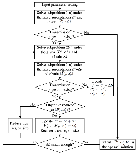
Figure 1: The algorithm flow chart.

Based on the proposed subproblems (16) and (24), we design an alternate iteration algorithm for the original problem (14). The solution procedure is presented below. The algorithm flow chart is also depicted in Fig. 1.

1. Parameter setting. Set input parameters $\mkern 3.5mu\overline{\mkern-3.5mu\bm{P}\mkern 0.0mu}\mkern 0.0mu_{d},\mkern 3.5mu\overline{\mkern-3.5mu\bm{P}\mkern 0.0mu}\mkern 0.0mu_{w},\bm{\Sigma}$; $a_{1,i},a_{2,i},\varepsilon_{i},P_{gi}^{\max},P_{gi}^{\min}$ for bus $i\in\mathcal{V}_{g}$; $b_{ij}^{\max},b_{ij}^{\min}$ for line $(i,j)\in\mathcal{E}_{\textup{flex}}$; $b_{ij}$ for line $(i,j)\in\mathcal{E}\backslash\mathcal{E}_{\textup{flex}}$ and $\varepsilon_{ij},f_{ij}^{\max}$ for line $(i,j)\in\mathcal{E}$. Set algorithm parameters $\delta>0$ (convergence criterion), $\Delta b_{ij}^{\max,0}>0$ (benchmark for trust-region size), $0<\beta<1$ (reduction factor for trust region). Let $\Delta b_{ij}^{\max}=\Delta b_{ij}^{\max,0}$ be the initial trust-region size, and $\bm{b}^{*}$ be the initial line susceptances.

2. Initial solution. Solve subproblem (16) under the fixed line susceptances $\bm{b}^{*}$, and obtain the solution $(\mkern 3.5mu\overline{\mkern-3.5mu\bm{P}\mkern 0.0mu}\mkern 0.0mu_{g}^{*},\bm{\alpha}_{g}^{*})$. If all the constraints (16h)-(16i) are not binding at $(\mkern 3.5mu\overline{\mkern-3.5mu\bm{P}\mkern 0.0mu}\mkern 0.0mu_{g}^{*},\bm{\alpha}_{g}^{*})$, stop the algorithm and output $(\mkern 3.5mu\overline{\mkern-3.5mu\bm{P}\mkern 0.0mu}\mkern 0.0mu_{g}^{*},\bm{\alpha}_{g}^{*},\bm{b}^{*})$ as the optimal solution.

3. Solve subproblem (24) under the profile $(\mkern 3.5mu\overline{\mkern-3.5mu\bm{P}\mkern 0.0mu}\mkern 0.0mu_{g}^{*},\bm{\alpha}_{g}^{*})$ and obtain the line susceptance adjustment $\Delta\bm{b}$.

4. Solve subproblem (16) under the fixed line susceptances $\bm{b}^{*}+\Delta\bm{b}$, and obtain the tentative solution, say $(\mkern 3.5mu\overline{\mkern-3.5mu\bm{P}\mkern 0.0mu}\mkern 0.0mu_{g}^{\prime},\bm{\alpha}_{g}^{\prime})$.

5. If all the constraints (16h)-(16i) are not binding at $(\mkern 3.5mu\overline{\mkern-3.5mu\bm{P}\mkern 0.0mu}\mkern 0.0mu_{g}^{\prime},\bm{\alpha}_{g}^{\prime})$, update the solution $\bm{b}^{*}\leftarrow\bm{b}^{*}+\Delta\bm{b}$, $\mkern 3.5mu\overline{\mkern-3.5mu\bm{P}\mkern 0.0mu}\mkern 0.0mu_{g}^{*}\leftarrow\mkern 3.5mu\overline{\mkern-3.5mu\bm{P}\mkern 0.0mu}\mkern 0.0mu_{g}^{\prime}$, $\bm{\alpha}_{g}^{*}\leftarrow\bm{\alpha}_{g}^{\prime}$, stop the algorithm and output $(\mkern 3.5mu\overline{\mkern-3.5mu\bm{P}\mkern 0.0mu}\mkern 0.0mu_{g}^{*},\bm{\alpha}_{g}^{*},\bm{b}^{*})$ as the optimal solution.

6. If $h(\mkern 3.5mu\overline{\mkern-3.5mu\bm{P}\mkern 0.0mu}\mkern 0.0mu_{g}^{\prime},\bm{\alpha}_{g}^{\prime})>h(\mkern 3.5mu\overline{\mkern-3.5mu\bm{P}\mkern 0.0mu}\mkern 0.0mu_{g}^{*},\bm{\alpha}_{g}^{*})$, the tentative solution is aborted, reduce the trust-region size by $\Delta b_{ij}^{\max}\leftarrow\beta\Delta b_{ij}^{\max}$. Go back to Step 3.
   If $h(\mkern 3.5mu\overline{\mkern-3.5mu\bm{P}\mkern 0.0mu}\mkern 0.0mu_{g}^{\prime},\bm{\alpha}_{g}^{\prime})\leq h(\mkern 3.5mu\overline{\mkern-3.5mu\bm{P}\mkern 0.0mu}\mkern 0.0mu_{g}^{*},\bm{\alpha}_{g}^{*})$, the susceptance adjustment $\Delta\bm{b}$ is accepted, update the solution $\bm{b}^{*}\leftarrow\bm{b}^{*}+\Delta\bm{b}$, $\mkern 3.5mu\overline{\mkern-3.5mu\bm{P}\mkern 0.0mu}\mkern 0.0mu_{g}^{*}\leftarrow\mkern 3.5mu\overline{\mkern-3.5mu\bm{P}\mkern 0.0mu}\mkern 0.0mu_{g}^{\prime}$, $\bm{\alpha}_{g}^{*}\leftarrow\bm{\alpha}_{g}^{\prime}$ and recover the trust-region size $\Delta b_{ij}^{\max}\leftarrow\Delta b_{ij}^{\max,0}$. Further, if $|\Delta b_{ij}|<\delta$, $\forall(i,j)\in\mathcal{E}_{\textup{flex}}$, stop the algorithm and output $(\mkern 3.5mu\overline{\mkern-3.5mu\bm{P}\mkern 0.0mu}\mkern 0.0mu_{g}^{*},\bm{\alpha}_{g}^{*},\bm{b}^{*})$ as the optimal solution; otherwise go back to Step 3.

We further explain the classification in Step 6. The inequality $h(\mkern 3.5mu\overline{\mkern-3.5mu\bm{P}\mkern 0.0mu}\mkern 0.0mu_{g}^{\prime},\bm{\alpha}_{g}^{\prime})>h(\mkern 3.5mu\overline{\mkern-3.5mu\bm{P}\mkern 0.0mu}\mkern 0.0mu_{g}^{*},\bm{\alpha}_{g}^{*})$ implies that subproblem (24) does not provide a correct susceptance adjustment, which is possibly due to that the trust-region size is too large to guarantee the validity of sensitivity analysis. In this case, we need to solve subproblem (24) again with a reduced trust-region size. The inequality $h(\mkern 3.5mu\overline{\mkern-3.5mu\bm{P}\mkern 0.0mu}\mkern 0.0mu_{g}^{\prime},\bm{\alpha}_{g}^{\prime})\leq h(\mkern 3.5mu\overline{\mkern-3.5mu\bm{P}\mkern 0.0mu}\mkern 0.0mu_{g}^{*},\bm{\alpha}_{g}^{*})$ implies that the operational cost is reduced as expected after applying the susceptance adjustment $\Delta\bm{b}$, and hence $\bm{b}^{*}$ is updated to $\bm{b}^{*}+\Delta\bm{b}$.

According to the stop criteria in the algorithm, the final output of this algorithm, say $(\mkern 3.5mu\overline{\mkern-3.5mu\bm{P}\mkern 0.0mu}\mkern 0.0mu_{g}^{\textup{opt}},\bm{\alpha}_{g}^{\textup{opt}},\bm{b}^{\textup{opt}})$, have two types of physical meanings. If the algorithm is stopped in Step 2 or Step 5, then $(\mkern 3.5mu\overline{\mkern-3.5mu\bm{P}\mkern 0.0mu}\mkern 0.0mu_{g}^{\textup{opt}},\bm{\alpha}_{g}^{\textup{opt}},\bm{b}^{\textup{opt}})$ fully eliminates transmission congestion, which is desirable. If the algorithm is stopped in Step 6, then $(\mkern 3.5mu\overline{\mkern-3.5mu\bm{P}\mkern 0.0mu}\mkern 0.0mu_{g}^{\textup{opt}},\bm{\alpha}_{g}^{\textup{opt}})$ and $\bm{b}^{\textup{opt}}$ reach the following matching state though transmission congestion is not fully eliminated. On one hand, under the power network structure $\bm{b}^{\textup{opt}}$, any change on $(\mkern 3.5mu\overline{\mkern-3.5mu\bm{P}\mkern 0.0mu}\mkern 0.0mu_{g}^{\textup{opt}},\bm{\alpha}_{g}^{\textup{opt}})$ cannot decrease the operational cost. On the other hand, under the generations $\mkern 3.5mu\overline{\mkern-3.5mu\bm{P}\mkern 0.0mu}\mkern 0.0mu_{g}^{\textup{opt}}$ and participation factors $\bm{\alpha}_{g}^{\textup{opt}}$, the congestion cannot be further mitigated by changing $\bm{b}^{\textup{opt}}$. Therefore, the capabilities of generations, participation factors and line susceptances in CCED have been fully exploited.

Another merit of the proposed algorithm is that each accepted solution $(\mkern 3.5mu\overline{\mkern-3.5mu\bm{P}\mkern 0.0mu}\mkern 0.0mu_{g}^{*},\bm{\alpha}_{g}^{*},\bm{b}^{*})$ generated during the iteration is a feasible solution to problem (14) and has a lower objective value than the previous one. Thus, even when the algorithm has not yet converged, we can still apply the latest accepted solution for system dispatch to improve the operational economy. This feature makes the algorithm more friendly to the real-time implementation where a satisfactory dispatch scheme needs to be obtained within a rather limited period of time.

IV Case study

We take the IEEE 14-bus system and IEEE 118-bus system to test the proposed method, where it will be observed that network flexibility can help to fully eliminate transmission congestion in small systems and significantly reduce congestion in large systems. We refer to the MATPOWER package [26] for the parameters of these two systems.

IV-A IEEE 14: congestion fully eliminated after optimization

Based on the original parameter profile of IEEE 14-bus system, we further adopt the following settings for our tests.

• Loads and dispatchable generations. There are five dispatchable generators $\mathcal{V}_{g}=\{1,2,3,6,8\}$. To highlight the control effect, we double the values of loads and generation capacities in  [26].

• Renewable generations. Assume that buses 1, 3, 6, 9 have renewable generators and the load data represents the net loads, i.e., the consumptions deducted by renewable generations. The covariance matrix for renewable uncertainties takes value as $\bm{\Sigma}=\textup{diag}\{\Sigma_{i}\}\in\mathbb{R}^{14\times 14}$, where $\Sigma_{i}=0.05$ p.u. for $i=1,3,6,9$ and otherwise $\Sigma_{i}=0$.

• Lines. Assume $\mathcal{E}_{\textup{flex}}=\{(1,5),(2,3),(6,11)\}$. The flexible susceptance is realized by a constant susceptance $b_{ij}^{\textup{rated}}$ in series with an adjustable susceptance $b_{ij}^{c}$ such that $|b_{ij}^{\textup{rated}}/b_{ij}^{c}|\leq d_{ij}$, where $d_{ij}$ is called the degree of flexibility. Thus, for any $(i,j)\in\mathcal{E}_{\textup{flex}}$ we have

  $$\begin{split}b_{ij}^{\min}=\frac{b_{ij}^{\textup{rated}}}{1+d_{ij}},\leavevmode\nobreak\ b_{ij}^{\max}=\frac{b_{ij}^{\textup{rated}}}{1-d_{ij}}.\end{split}$$ (25)

  Here we take $d_{ij}=0.7$, $\forall(i,j)\in\mathcal{E}_{\textup{flex}}$. For line capacity, we set $f_{ij}^{\max}=140$MW for line (1,2), $f_{ij}^{\max}=100$MW for line (7,9), and $f_{ij}^{\max}=200$MW for all the other lines.

• CCED and algorithm parameters. In subproblem (16), we set $c_{i}=c_{ij}=2.326$ (corresponding to $\varepsilon_{i}=\varepsilon_{ij}=0.01$ for the original problem (5)). In subproblem (24), we set $\Delta b_{ij}^{\max,0}=0.3b_{ij}^{\textup{rated}}$, $\forall(i,j)\in\mathcal{E}_{\textup{flex}}$. In the algorithm, we take the rated line susceptances to be the initial values, and $\delta=10^{-4},\beta=0.1$.

With the above settings, we obtain the following four solutions for comparison.

• S1: CCED with network flexibility, which is obtained by solving (14) using the proposed algorithm.

• S2: CCED without network flexibility, which is the first solution during the iteration for obtaining S1.

• S3: Normal ED with network flexibility, which is obtained by solving (14) using the proposed algorithm with $\bm{\Sigma}=\bm{0}$.

• S4: Normal ED without network flexibility, which is the first solution during the iteration for obtaining S3.

Before looking into these four solutions, let us first detail the process of finding S1 to verify the proposed algorithm. During the iteration, the generation constraints are not binding, while two lines (1,2) and (7,9) are congested at the first solution. Then the susceptances of lines $\mathcal{E}_{\textup{flex}}$ start to adjust to address the congestion. The blue and red curves in Fig. 2 respectively shows the trajectories of dual variables of the binding flow constraints with respect to lines (1,2) and (7,9). We observe that the two dual variables are decreasing with the iteration, which implies that the congestion is being gradually mitigated. After eight iterations, these two dual variables become zero, and hence the congestion is fully cleared and the algorithm stops. In the meantime, the generation cost (i.e., objective value), which is denoted by the black curve in Fig. 2, decreases from 18578.8$/h to 18186.4$/h, which achieves 2.1% cost reduction.

We now check the performances of the four solutions to show the merits of network flexibility. Since the size of IEEE 14-bus system is rather small, it is convenient to present the comprehensive information of the solutions in Table II, Table III and Table IV. We have some interesting results from the following comparisons.

1) $\mkern 3.5mu\overline{\mkern-3.5muP\mkern 0.0mu}\mkern 0.0mu_{gi}$ at S1 and S2. As network flexibility helps to mitigate transmission congestion under renewable uncertainties, the dispatchable generator at bus 1, which are more cost-effective, are better utilized to output more power at S1 than S2.

2) $\mkern 3.5mu\overline{\mkern-3.5muP\mkern 0.0mu}\mkern 0.0mu_{gi}$ at S1 and S3. S1 and S3 both consider network flexibility. Additionally, S1 considers renewable uncertainties that shrink the usable line capacities (see (15)). However, the values of $\mkern 3.5mu\overline{\mkern-3.5muP\mkern 0.0mu}\mkern 0.0mu_{gi}$ at S1 and S3 are nearly identical, which implies that the network flexibility eliminates the impact of renewable uncertainties. With network flexibility, the generation cost keeps almost unchanged after including renewable uncertainties, except for the additional term $s_{\Sigma}^{2}\bm{\alpha}_{g}^{T}\bm{a}_{2}\bm{\alpha}_{g}$ caused by participation factors which is slight.

3) $\mkern 3.5mu\overline{\mkern-3.5muP\mkern 0.0mu}\mkern 0.0mu_{gi}$ at S2 and S4. S2 and S4 both exclude network flexibility. Additionally, S2 considers renewable uncertainties. Compared to the generation profile at S4, S2 cannot resort to network flexibility and has to sacrifice those cost-effective generations in order to satisfy the line flow chance constraints.

Table V further shows the generation costs of these four solutions. The cost difference between S1 and S3 (6.1$/h) and the cost difference between S2 and S4 (290.9$/h) can be interpreted as the cost of uncertainty. The cost difference between S1 and S2 (392.4$/h) and the cost difference between S3 and S4 (107.6$/h) can be interpreted as the cost of network non-flexibility. We make some important observations from these cost data. According to the fourth column of Table V, network flexibility helps to greatly save generation cost by congestion mitigation no matter renewable uncertainties are included or not. According to the third column of Table V, renewable uncertainties cause much more additional generation cost when network flexibility is unavailable. Overall, network flexibility has been shown to significantly improve operational economy specially under renewable uncertainties.

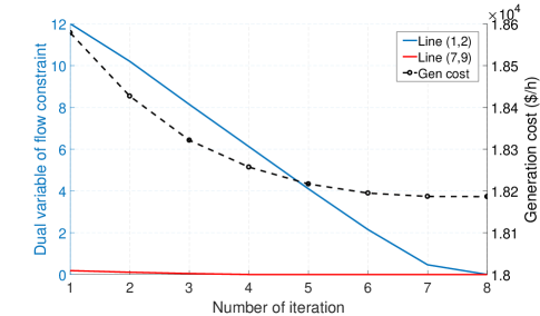
Figure 2: IEEE 14: Generation costs and dual variables of flow constraints during the iteration.

Table II: IEEE 14: Generation info of CCED with/without network flexibility (in MW)

Gen. $i$	$a_{2i}$	$a_{1i}$	$\mkern 3.5mu\overline{\mkern-3.5muP\mkern 0.0mu}\mkern 0.0mu_{gi}$ at S1	$\alpha_{gi}$ at S1	$\mkern 3.5mu\overline{\mkern-3.5muP\mkern 0.0mu}\mkern 0.0mu_{gi}$ at S2	$\alpha_{gi}$ at S2
1	4.3	20	249.84	0.07	161.76	0.23
2	25	20	43.00	0.00	47.98	0.00
3	1	40	75.05	0.31	144.36	0.20
6	1	40	75.05	0.31	76.41	0.39
8	1	40	75.06	0.31	87.49	0.18

Table III: IEEE 14: Line susceptance info of CCED with/without network flexibility (in p.u.)

Line $(i,j)$	$b_{ij}^{\textup{rated}}$	$b_{ij}^{\min}$	$b_{ij}^{\max}$	$b_{ij}$ at S1	$b_{ij}$ at S3
(1,5)	4.48	2.64	14.95	13.90	8.52
(2,3)	5.05	2.97	16.84	2.97	2.97
(6,11)	5.03	2.96	16.76	15.59	9.55

Table IV: IEEE 14: Generation info of normal ED with/without network flexibility (in MW)

Gen. $i$	$a_{2i}$	$a_{1i}$	$\mkern 3.5mu\overline{\mkern-3.5muP\mkern 0.0mu}\mkern 0.0mu_{gi}$ at S3	$\mkern 3.5mu\overline{\mkern-3.5muP\mkern 0.0mu}\mkern 0.0mu_{gi}$ at S4
1	4.3	20	249.84	203.57
2	25	20	43.00	45.60
3	1	40	75.05	111.24
6	1	40	75.05	74.48
8	1	40	75.05	83.11

Table V: IEEE 14: Comparison of generation costs (in $/h) with/without network flexibility or renewable uncertainty

Solution	Gen. cost	Cost of uncer.1	Cost of no NF1
ED with NF (S3)	18180.3	0	0
CCED with NF (S1)	18186.4	6.1 (S1-S3)	0
ED without NF (S4)	18287.9	0	107.6 (S4-S3)
CCED without NF (S2)	18578.8	290.9 (S2-S4)	392.4 (S2-S1)

• Uncer. is short for renewable uncertainty.

• NF is short for network flexibility.

IV-B IEEE 118: congestion mitigated after optimization

We turn to IEEE 118-bus system to show that the proposed method also works well in large systems. Based on the original parameter profile of the system, we further adopt the following settings for our tests.

• Loads and dispatchable generations. There are 54 dispatchable generators. To highlight the control effect, we double the values of loads and generation capacities in [26].

• Renewable generations. Assume that buses 3, 8, 11, 20, 24, 26, 31, 38, 43, 49, 53 have renewable generators and the load data represents the net loads. The covariance matrix for renewable uncertainties takes value as $\bm{\Sigma}=\textup{diag}\{\Sigma_{i}\}\in\mathbb{R}^{14\times 14}$, where $\Sigma_{i}=0.05$ p.u. if bus $i$ has a renewable generator and otherwise $\Sigma_{i}=0$.

• Lines. Assume nine lines have flexible susceptances $\mathcal{E}_{\textup{flex}}=\{(13,15),(26,30),(46,48),(49,54),(54,59),$ $(59,61),(64,65),(47,69),(69,77)\}$. Similar to the test on the IEEE 14-bus system, these susceptances have the degree of flexibility $d_{ij}=0.7$, $\forall(i,j)\in\mathcal{E}_{\textup{flex}}$. For line capacity, we set $f_{ij}^{\max}=100$MW for lines (8,9), (8,5), (60,61), (63,64), and $f_{ij}^{\max}=200$MW for all the other lines.

• CCED and algorithm parameters. The setting is identical to the test on the IEEE 14-bus system.

Again, we obtain the following four solutions for analysis.

• S1: CCED with network flexibility.

• S2: CCED without network flexibility.

• S3: Normal ED with network flexibility.

• S4: Normal ED without network flexibility.

We first check the iteration process of finding S1. Fig. 3 shows the trajectories of dual variables of the binding flow constraints with respect to some lines. Note that there are quite a few congested lines during the iteration. For simplicity, here we just plot those lines with rather severe congestion, i.e., the values of dual variables have ever been greater than 20 during the iteration. We observe that some dual variables have oscillation and some dual variables are even increasing during the iteration. However, the generation cost monotonically decreases (see the black curve in Fig. 3), which implies that the overall congestion is mitigated after each iteration. After ten iterations, the adjustment of line susceptances becomes sufficiently small and the algorithm stops. The generation cost finally decreases from 321570.9$/h to 310209.8$/h, i.e., 3.5% cost reduction. Although the congestion is not fully eliminated, the cost reduction is significant and hence S1 is satisfactory. Also note that the system has totally 186 lines and the reduction is achieved by assuming only nine lines to have flexible susceptances (less than 5% of lines).

We then compare the performances of the four solutions in Table VI. We have a similar observation to the test on the IEEE 14-bus system, i.e., the presence of network flexibility makes a great contribution to cost reduction especially when the system has high penetration of uncertain renewables. This again highlights the capability of network flexibility against the impact of renewable uncertainties on operational economy.

Moreover, the degree of network flexibility $d_{ij}$ also plays a role in the generation cost reduction and we have fixed it to be 0.7 so far. Fig. 4 shows how the generation cost of S1 changes with the degree of network flexibility. We observe that the cost decreases nearly linearly with the degree of flexibility. For this system, the degree of flexibility should be greater than 0.5 in order to achieve more than 2% cost reduction.

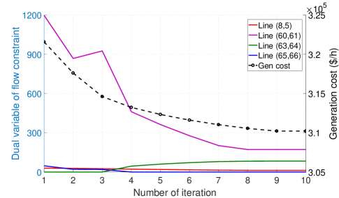
Figure 3: IEEE 118: Generation costs and dual variables of flow constraints during the iteration.

Table VI: IEEE 118: Comparison of generation costs (in $/h) with/without network flexibility or renewable uncertainty

Solution	Gen. cost	Cost of uncer.	Cost of no NF
ED with NF (S3)	309044.4	0	0
CCED with NF (S1)	310209.8	1165.4 (S1-S3)	0
ED without NF (S4)	317738.6	0	8694.2 (S4-S3)
CCED without NF (S2)	321570.9	3832.3 (S2-S4)	11361.1 (S2-S1)

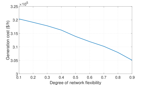
Figure 4: IEEE 118: Relationship between the generation cost of CCED and degree of network flexibility.

V Conclusion

Network flexibility has been incorporated into CCED problems to cope with the impact caused by renewable uncertainties. From the analytical form of the CCED problem, we have figured out how network flexibility play a role in the ED under uncertainties. The flexible line susceptances tune the base-case line flows and reduce the line capacities shrunk by uncertainties. Thus, network flexibility greatly contributes to transmission congestion mitigation and generation cost saving. Furthermore, we have proposed an efficient solver the CCED problem with network flexibility. Two convex subproblems with respect to generation variables and network variables are established using duality theory. Then alternately solving these two subproblems gives the solution to the original problem. Case studies have shown that the operational economy under uncertainties is much improved with the help of network flexibility.

References

- [1] A. J. Wood, B. F. Wollenberg, and G. B. Sheblé, Power Generation, Operation, and Control. John Wiley & Sons, 2013.
- [2] D. Bienstock, M. Chertkov, and S. Harnett, “Chance-constrained optimal power flow: Risk-aware network control under uncertainty,” Siam Rev., vol. 56, no. 3, pp. 461–495, 2014.
- [3] L. Roald, S. Misra, T. Krause, and G. Andersson, “Corrective control to handle forecast uncertainty: A chance constrained optimal power flow,” IEEE Trans. Power Syst., vol. 32, no. 2, pp. 1626–1637, Mar. 2017.
- [4] A. Venzke, L. Halilbasic, U. Markovic, G. Hug, and S. Chatzivasileiadis, “Convex relaxations of chance constrained AC optimal power flow,” IEEE Trans. Power Syst., vol. 33, no. 3, pp. 2829–2841, May 2018.
- [5] L. Roald and G. Andersson, “Chance-constrained AC optimal power flow: Reformulations and efficient algorithms,” IEEE Trans. Power Syst., vol. 33, no. 3, pp. 2906–2918, May 2017.
- [6] T. Mühlpfordt, L. Roald, V. Hagenmeyer, T. Faulwasser, and S. Misra, “Chance-constrained ac optimal power flow: A polynomial chaos approach,” IEEE Trans. Power Syst., vol. 34, no. 6, pp. 4806–4816, Nov. 2019.
- [7] C. Duan, W. Fang, L. Jiang, L. Yao, and J. Liu, “Distributionally robust chance-constrained approximate AC-OPF with wasserstein metric,” IEEE Trans. Power Syst., vol. 33, no. 5, pp. 4924–4936, Sep. 2018.
- [8] W. Xie and S. Ahmed, “Distributionally robust chance constrained optimal power flow with renewables: A conic reformulation,” IEEE Trans. Power Syst., vol. 33, no. 2, pp. 1860–1867, Mar. 2018.
- [9] B. K. Poolla, A. R. Hota, S. Bolognani, D. S. Callaway, and A. Cherukuri, “Wasserstein distributionally robust look-ahead economic dispatch,” IEEE Trans. Power Syst., vol. 36, no. 3, pp. 2010–2022, May 2021.
- [10] J. Li, F. Liu, Z. Li, C. Shao, and X. Liu, “Grid-side flexibility of power systems in integrating large-scale renewable generations: A critical review on concepts, formulations and solution approaches,” Renewable and Sustainable Energy Reviews, vol. 93, pp. 272–284, 2018.
- [11] E. B. Fisher, R. P. O’Neill, and M. C. Ferris, “Optimal transmission switching,” IEEE Trans. Power Syst., vol. 23, no. 3, pp. 1346–1355, 2008.
- [12] K. W. Hedman, R. P. O’Neill, E. B. Fisher, and S. S. Oren, “Optimal transmission switching—sensitivity analysis and extensions,” IEEE Trans. Power Syst., vol. 23, no. 3, pp. 1469–1479, 2008.
- [13] B. Kocuk, S. S. Dey, and X. A. Sun, “New formulation and strong MISOCP relaxations for AC optimal transmission switching problem,” IEEE Trans. Power Syst., vol. 32, no. 6, pp. 4161–4170, Nov. 2017.
- [14] T. Ding, R. Bo, F. Li, and H. Sun, “Optimal power flow with the consideration of flexible transmission line impedance,” IEEE Trans. Power Syst., vol. 31, no. 2, pp. 1655–1656, Mar. 2016.
- [15] M. Sahraei-Ardakani and K. W. Hedman, “Day-ahead corrective adjustment of FACTS reactance: A linear programming approach,” IEEE Trans. Power Syst., vol. 31, no. 4, pp. 2867–2875, Jul. 2016.
- [16] M. Sahraei-Ardakani and K. W. Hedman, “A fast LP approach for enhanced utilization of variable impedance based FACTS devices,” IEEE Trans. Power Syst., vol. 31, no. 3, pp. 2204–2213, May 2016.
- [17] Y. Sang, M. Sahraei-Ardakani, and M. Parvania, “Stochastic transmission impedance control for enhanced wind energy integration,” IEEE Trans. Sustain. Energy, vol. 9, no. 3, pp. 1108–1117, Jul. 2018.
- [18] J. Shi and S. S. Oren, “Stochastic unit commitment with topology control recourse for power systems with large-scale renewable integration,” IEEE Trans. Power Syst., vol. 33, no. 3, pp. 3315–3324, 2018.
- [19] A. C. Rencher and G. B. Schaalje, Linear Models in Statistics. John Wiley & Sons, 2008.
- [20] D. Bienstock and A. Shukla, “Variance-aware optimal power flow,” in Proc. Power Syst. Comput. Conf., 2018, pp. 1–8.
- [21] D. Bienstock and A. Shukla, “Variance-aware optimal power flow: Addressing the tradeoff between cost, security, and variability,” IEEE Trans. Control Netw. Syst., vol. 6, no. 3, pp. 1185–1196, Sep. 2019.
- [22] T. W. Gedra, “On transmission congestion and pricing,” IEEE Trans. Power Syst., vol. 14, no. 1, pp. 241–248, Feb. 1999.
- [23] K. B. Petersen and M. S. Pedersen, The Matrix Cookbook. Technical University of Denmark, 2008.
- [24] S. Boyd, S. P. Boyd, and L. Vandenberghe, Convex Optimization. Cambridge University Press, 2004.
- [25] A. J. Conejo, E. Castillo, R. Minguez, and R. Garcia-Bertrand, Decomposition Techniques in Mathematical Programming: Engineering and Science Applications. Springer, 2006.
- [26] R. D. Zimmerman, C. E. Murillo-Sánchez, and R. J. Thomas, “MATPOWER: Steady-state operations, planning, and analysis tools for power systems research and education,” IEEE Trans. Power Syst., vol. 26, no. 1, pp. 12–19, February 2011.