Optimal transport-based machine learning to match specific patterns: application to the detection of molecular regulation patterns in omics data

Abstract

We present several algorithms designed to learn a pattern of correspondence between two data sets in situations where it is desirable to match elements that exhibit a relationship belonging to a known parametric model. In the motivating case study, the challenge is to better understand micro-RNA regulation in the striatum of Huntington’s disease model mice.

The algorithms unfold in two stages. First, an optimal transport plan $P$ and an optimal affine transformation are learned, using the Sinkhorn-Knopp algorithm and a mini-batch gradient descent. Second, $P$ is exploited to derive either several co-clusters or several sets of matched elements.

A simulation study illustrates how the algorithms work and perform. The real data application further illustrates their applicability and interest.

Keywords. Co-clustering; omics data; Huntington’s disease; matching; optimal transport; Sinkhorn algorithm; Sinkhorn loss.

1 Introduction

The analysis of numerous omics data is a challenging task in biological research [5] and disease research [16, 21]. In disease research, omics data are increasingly available for the analysis of molecular pathology. This is notably illustrated by research on Huntington’s Disease (HD): messenger-RNA (mRNA), micro-RNA (miRNA), protein data collectively quantifying several layers of molecular regulation in the brain of HD model knock-in mice [16, 17] now compose one of the largest data set available to date to understand how neurodegenerative processes may work on a systems level. The data set is publicly available through the database repository Gene Expression Omnibus (GEO) and the HDinHD portal.

Encouraged by the promising findings of [22], our ultimate goal is to shed light on the interaction between mRNAs and miRNAs based on data collected in the striatum (a brain region) of HD model knock-in mice [16, 17]. Each data point takes the form of multi-dimensional profile. The strong biological hypothesis is that if a miRNA induces the degradation of a target mRNA or blocks its translation into proteins, or both, then the profile of the former, say $y$, should be similar to minus the profile of the latter, say $-x$. We relax the hypothesis and consider that $y$ is similar to $\theta(x)$ where $\theta$ is an affine transformation in a parametric class $\Theta$ that includes minus the identity and whose definition translates expert knowledge about the experiment that yields the data. Our study straightforwardly extends to the case that the relationship is known to belong to any parametric model. In order to identify groups of mRNAs and miRNAs that interact, we develop a co-clustering algorithm and a matching algorithm based on optimal transport [26], spectral and block co-clustering, and a matching procedure tailored to our needs.

Spectral co-clustering [9] and block clustering [7, 13] are two ways among many others to carry out co-clustering, an unsupervised learning task to cluster simultaneously the rows and columns of a matrix in order to obtain homogeneous blocks. There are many efficient approaches to solving the problem, often characterized as model-based or metric-based methods [28].

In an enlightening article, Nazarov and Kreis [23] review a variety of computational approaches to study how miRNAs “come together to regulate the expression of a gene or a group of genes”. They identify three different families of methods: data-driven methods based on similarities, data-driven methods based on matrix factorization, and hybrid methods. Our algorithms belong to the first family. In view of [23, Section 2.5 and Fig. 2], we do not rely on the standard similarity measures (Pearson and Spearman correlation coefficients; cosine similarity; mutual information) to define our similarity matrix but, instead, use optimal transport to derive it. Moreover, as in canonical correlation analysis, we do not compare the raw mRNA and miRNA profiles $x,y$ but, instead, we compare a data-driven transformation $\theta(x)$ and $y$, where $\theta$ is an affine transformation of $x$. Finally, as explained by Nazarov and Kreis [23], our algorithms cannot discriminate between true interactions and fake interactions originating from common hidden regulators such as transcription factors. It is necessary to conduct a further biological analysis to identify the relevant findings.

The rest of the article is organized as follows. Section 2 describes the data we use. Section 3 presents a modicum of optimal transport theory. Section 4 introduces our algorithms. Section 5 evaluates the performances of the algorithms in various simulation settings. Section 6 illustrates the real data application. Section 7 closes the study on a discussion.

2 Data

2.1 Presentation

The data analyzed herein cover RNA-seq data obtained in the striatum of the allelic series of HD knock-in mice (poly Q lengths: Q20, Q80, Q92, Q111, Q140, Q175) at 2-month, 6-month and 10-month of age. For each combination of poly Q length and age, 8 mice were sacrificed (4 females and 4 males). After preprocessing [22, Methods section], the final data set consists of $M=13,616$ mRNA profiles, $X:=\{x_{1},\ldots,x_{M}\}\subset\mathbb{R}^{d}$, and in $N=1,143$ miRNA profiles, $Y:=\{y_{1},\ldots,y_{N}\}\subset\mathbb{R}^{d}$ with $d=15$.

Informally, we look for couples $(m,n)\in\llbracket M\rrbracket\times\llbracket N\rrbracket:=\{1,\ldots,M\}\times\{1,\ldots,N\}$ such that the $n$th miRNA induces the degradation of the $m$th mRNA or blocks its translation into proteins, or both. We are guided by the strong biological hypothesis that, if that is the case, then the profile $y_{n}$ of the former is similar to minus the profile $x_{m}$ of the latter – then $x_{m}$ and $y_{n}$ exhibit what we call a mirroring relationship. Of note, it is expected that a single miRNA can target several mRNAs.

The actual mirroring relationships can be more or less acute, for instance because of threshold effects, or of multiple miRNAs targeting the same mRNA, or of a single miRNA targeting several mRNAs. Therefore, instead of rigidly using comparisons between $-x_{m}$ and $y_{n}$, our algorithms will learn from the data a relevant transformation $\theta\in\Theta$ (in a parametric class $\Theta$ of transformations that includes minus the identity) and use comparisons between $\theta(x_{m})$ and $y_{n}$.

Figure 1 exhibits two profiles $x_{m}$ and $y_{n}$ that showcase a mirrored similarity. The corresponding miRNA and mRNA, Mir20b (which may inhibit cerebral ischemia-induced inflammation in rats [33]) and the Aryl-Hydrocarbon Receptor Repressor (Ahrr), are believed to interact in the striatum of HD model knock-in mice [22].

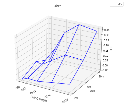
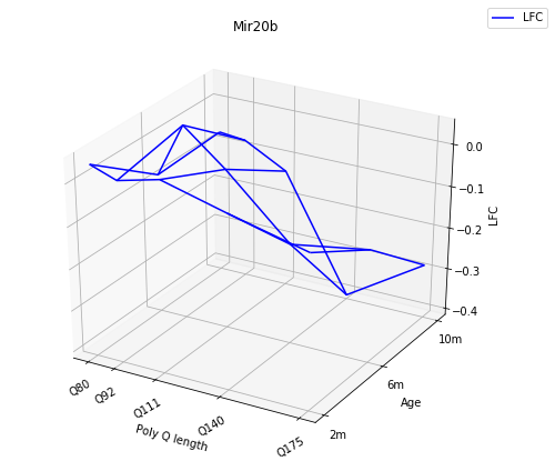
Figure 1: Left: profile $x_{m}$ of a mRNA (Ahrr). Right: profile $y_{n}$ of a miRNA (Mir20b). It is believed that Mir20b targets Ahrr.

2.2 A brief data analysis

So as to give a sense of the distribution of the data, we propose two kinds of visual summaries. The first one uses Lloyd’s $k$-means algorithm [20] to build synthetic profiles representing the real profiles $x_{1},\ldots,x_{M}$ on the one hand and $y_{1},\ldots,y_{N}$ on the other hand. The second one uses kernel density estimators of the $j$-th component of $x_{1},\ldots,x_{M}$ on the one hand and of $y_{1},\ldots,y_{N}$ on the other hand, for each $1\leq j\leq d$.

2.2.1 Using $\boldsymbol{k}$-means to cluster the mRNA and miRNA profiles

In Figure 2 we plot the synthetic mRNA profiles $\hat{x}_{1},\ldots,\hat{x}_{5}$ of the 5 centroids obtained by running Lloyd’s $k$-means algorithm on $x_{1},\ldots,x_{M}$ with $k=5$. Likewise, we plot in Figure 3 the synthetic miRNA profiles $\hat{y}_{1},\ldots,\hat{y}_{5}$ of the 5 centroids obtained by running Lloyd’s $k$-means algorithm on $y_{1},\ldots,y_{N}$ with $k=5$.

The 5 mRNA centroids correspond to 5319 ($\hat{x}_{1}$), 2097 ($\hat{x}_{2}$), 4688 ($\hat{x}_{3}$), 310 ($\hat{x}_{4}$) and 1202 ($\hat{x}_{5}$) mRNA profiles. The first and third centroids ($\hat{x}_{1}$ and $\hat{x}_{3}$), which represent 73% of the real mRNA profiles, are rather flat. The second and fourth centroids ($\hat{x}_{2}$ and $\hat{x}_{4}$), which represent 18% of the real mRNA profiles, are decreasing in poly Q length and age, in a more pronounced way for the latter than for the former. Finally, the fifth centroid ($\hat{x}_{5}$), which represents the remaining 9% of real mRNA profiles, is increasing in poly Q length and age.

The 5 miRNA centroids correspond to 872 ($\hat{y}_{1}$), 7 ($\hat{y}_{2}$), 80 ($\hat{y}_{3}$), 81 ($\hat{y}_{4}$) and 103 ($\hat{y}_{5}$) miRNA profiles. The first centroid ($\hat{y}_{1}$), which represents 76% of the real miRNA profiles, is rather flat. The second and fifth centroids ($\hat{y}_{2}$ and $\hat{y}_{5}$), which represent 10% of the real miRNA profiles, are increasing in poly Q length and age, in a more pronounced way for the former than for the latter. The fourth centroid ($\hat{y}_{4}$), which represents 7% of the real miRNA profiles, is decreasing in poly Q length and age. Finally, the third centroid ($\hat{y}_{3}$), which represents 7% of the real miRNA profiles, exhibits two peaks.

In Section 1, we stated the following biological hypothesis: if a miRNA induces the degradation of a target mRNA or blocks its translation into proteins, or both, then the profile of the former should be similar to minus the profile of the latter (a particular form of affine relationship). In view of this hypothesis, it is tempting to relate the synthetic miRNA profiles $\hat{y}_{2}$ and $\hat{y}_{5}$ to the synthetic mRNA profiles $\hat{x}_{4}$ and $\hat{x}_{2}$, respectively, and the synthetic miRNA profile $\hat{y}_{4}$ to the synthetic mRNA profile $\hat{x}_{5}$. Our objective is to identify groups of real mRNA and miRNA profiles that interact in this manner.

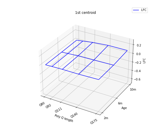
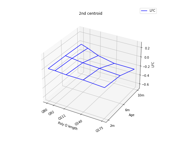
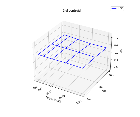
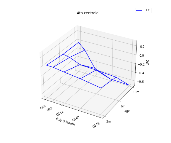
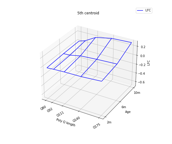
Figure 2: Profiles $\hat{x}_{1},\ldots,\hat{x}_{5}$ of the 5 centroids obtained by Lloyd’s $k$-means algorithm on the mRNA profiles $x_{1},\ldots,x_{M}$.

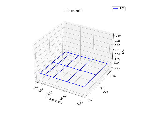
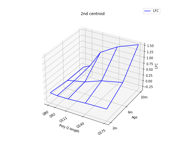
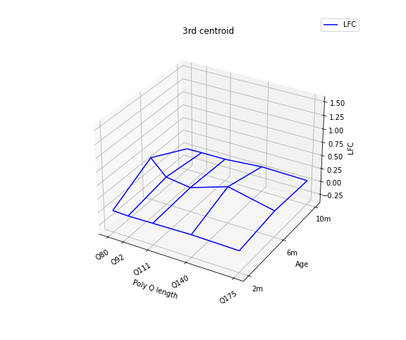
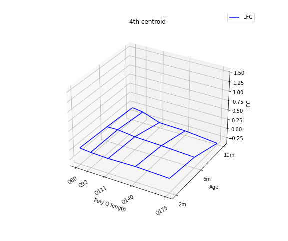
Figure 3: Profiles $\hat{y}_{1},\ldots,\hat{y}_{5}$ of the 5 centroids obtained by running Lloyd’s $k$-means algorithm on the miRNA profiles $y_{1},\ldots,y_{N}$.

2.2.2 Using kernel density estimators to study the marginal distributions of the mRNA and miRNA profiles

For each $1\leq j\leq d$, we build the kernel density estimator of the $j$-th component of the mRNA profiles $x_{1},\ldots,x_{M}$, using a Gaussian kernel and the default fine-tuning of the density function from the stats R-package [29], see Figure 4. We do the same for the miRNA profiles $y_{1},\ldots,y_{N}$, see Figure 5. Both for mRNA and miRNA the kernel density estimates are systematically more concentrated around their means (all close to 0) than the corresponding Gaussian densities. Moreover, the kernel density estimates obtained from the $M$ mRNA profiles are much smoother than those obtained from $N$ miRNA profiles, a feature that could be simply explained by the fact that $M/N>11$.

Table 1 reports, for each level of poly Q length (Q80, Q92, Q111, Q140, Q175) and age (2, 6, 10 months), the empirical standard deviation of mRNA (a) and miRNA (b) gene expressions, all normalized by the empirical standard deviation at poly Q length Q80 and 2 months of age (that is, by 0.0475 for mRNA and 0.0660 for miRNA). A clear pattern emerges from sub-Table 1 (a): except for poly Q length Q80, the poly Q length-specific empirical standard deviation increases as age increases. Likewise, except for age 2 months, the age-specific empirical standard deviation increases as poly Q length increases. On the contrary, no clear pattern emerges from sub-Table 1 (b) but the fact that, except for poly Q lengths Q80 and Q92, the poly Q length-specific empirical standard deviation increases as age increases. We do not comment on the empirical means because they are all very small compared to the corresponding empirical standard deviations.

poly Q length	Age $2$	Age $6$	Age $10$
Q80	$1$	$0.646$	$1.39$
Q92	$0.886$	$1.02$	$1.48$
Q111	$0.964$	$1.21$	$3.08$
Q140	$0.805$	$1.70$	$4.11$
Q175	$1.24$	$1.86$	$4.32$

(a) mRNA

poly Q length	Age $2$	Age $6$	Age $10$
Q80	$1$	$2.35$	$1.03$
Q92	$0.516$	$1.06$	$0.956$
Q111	$0.655$	$0.722$	$2.15$
Q140	$0.698$	$1.92$	$2.72$
Q175	$0.588$	$1.80$	$3.34$

(b) miRNA

Table 1: For each level of poly Q length (Q80, Q92, Q111, Q140, Q175) and age (2, 6, 10 months) we computed the empirical standard deviation of mRNA (a) and miRNA (b) gene expressions, all normalized by the empirical standard deviation at poly Q length Q80 and 2 months of age (that is, by 0.0475 for mRNA and 0.0660 for miRNA).

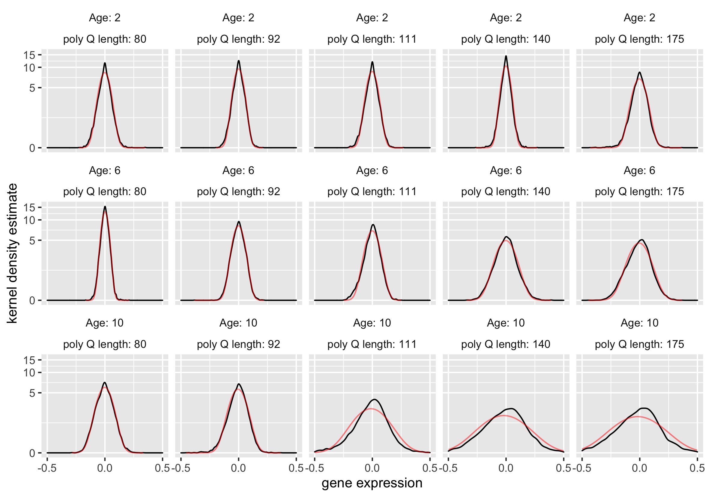
Figure 4: In black, kernel density estimates of the densities of mRNA gene expression for each level of poly Q length (Q80, Q92, Q111, Q140, Q175) and age (2, 6, 10 months), zooming on the interval $[-0.5,0.5]$ and using a $\log(1+\cdot)$-scale on the $y$-axis. In red, densities of the Gaussian laws with a mean and a variance equal to the empirical mean and variance computed in each stratum of data. Systematically, the kernel density estimates are more concentrated around their means than the corresponding Gaussian densities.

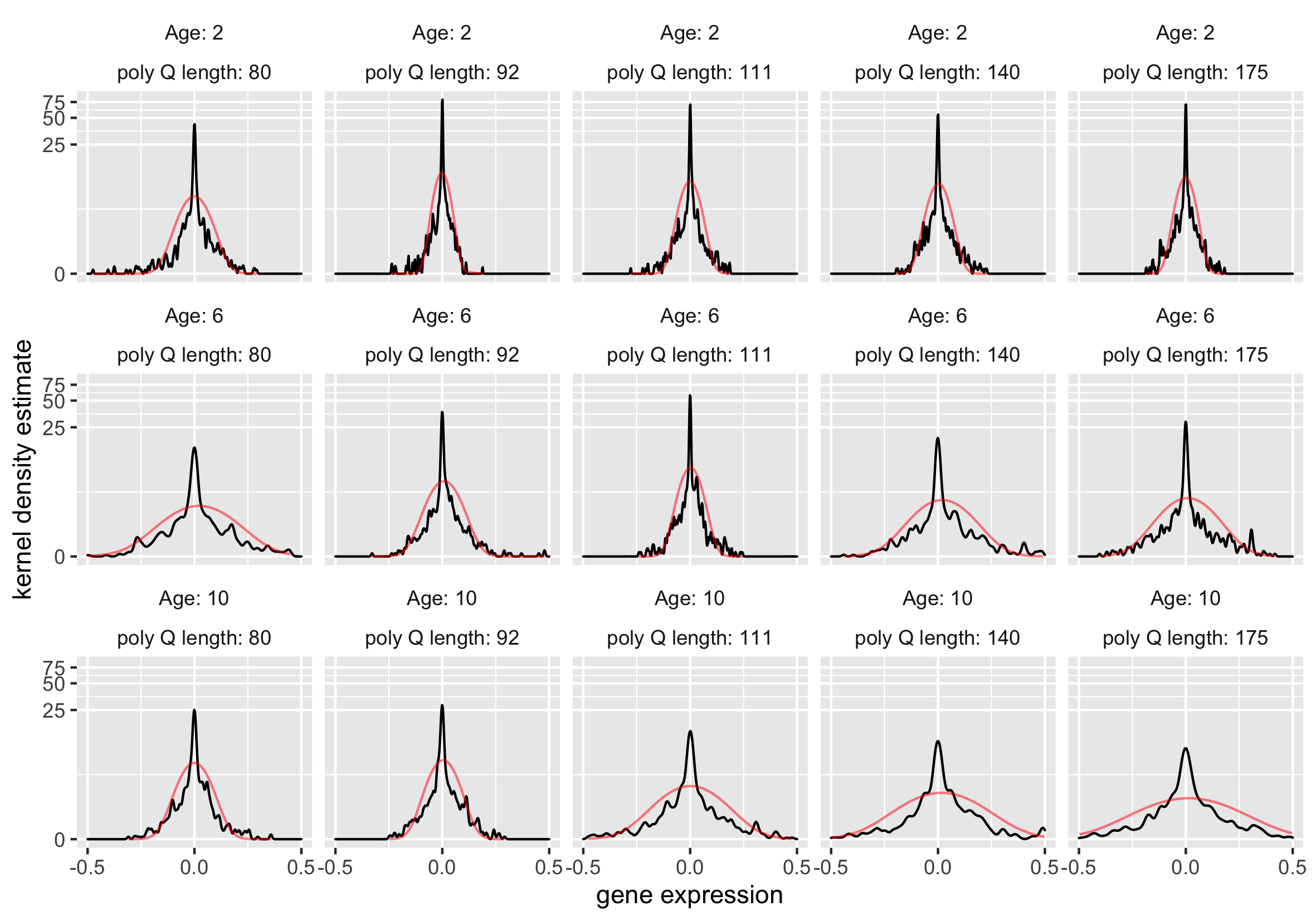
Figure 5: In black, kernel density estimates of the densities of miRNA gene expression for each level of poly Q length (Q80, Q92, Q111, Q140, Q175) and age (2, 6, 10 months), zooming on the interval $[-0.5,0.5]$ and using a $\log(1+\cdot)$-scale on the $y$-axis. In red, densities of the Gaussian laws with a mean and a variance equal to the empirical mean and variance computed in each stratum of data. Systematically, the kernel density estimates are more concentrated around their means than the corresponding Gaussian densities.

3 Elements of optimal transport

Let $\Omega:=\{\omega\in(\mathbb{R}_{+})^{M}|\sum_{m\in\llbracket M\rrbracket}\omega_{m}=1\}$ be the $(M-1)$-dimensional simplex and $\bar{\omega}:=M^{-1}\mathbf{1}_{M}$, where $\mathbf{1}_{M}\in\mathbb{R}^{M}$ is the vector with all its entries equal to 1. For any $\omega\in\Omega$, define

$$\Pi(\omega):=\{P\in(\mathbb{R}_{+})^{M\times N}|P\mathbf{1}_{N}=\omega,P^{\top}\mathbf{1}_{M}=N^{-1}\mathbf{1}_{N}\}$$

and let $\mu_{X}^{\omega}:=\sum_{m\in\llbracket M\rrbracket}\omega_{m}\delta_{x_{m}}$, $\nu_{Y}:=N^{-1}\sum_{n\in\llbracket N\rrbracket}\delta_{y_{n}}$ be the $\omega$-weighted empirical measure attached to $X$ and the empirical measure attached to $Y$. An element $P$ of $\Pi(\omega)$ represents a joint law on $X\times Y$ with marginals $\mu_{X}^{\omega}$ and $\nu_{Y}$.

The celebrated Monge-Kantorovich problem [26, Chapter 2] consists in finding a joint law over $X\times Y$ with marginals $\mu_{X}^{\bar{\omega}}$ and $\nu_{Y}$ that minimizes the expected cost of transport with respect to some cost function $c:\mathbb{R}^{d}\times\mathbb{R}^{d}\rightarrow\mathbb{R}_{+}$. We focus on $c$ given by $c(x,y):=\|x-y\|_{2}^{2}$ (the squared Euclidean norm in $\mathbb{R}^{d}$). Specifically, denoting $C_{X,Y}\in\mathbb{R}^{M\times N}$ the cost matrix given by $(C_{X,Y})_{mn}:=c(x_{m},y_{n})$ for each $(m,n)\in\llbracket M\rrbracket\times\llbracket N\rrbracket$, the problem consists in solving $\min_{P\in\Pi(\bar{\omega})}\langle C_{X,Y},P\rangle_{F}$ where $\langle C_{X,Y},P\rangle_{F}:=\sum_{(m,n)\in\llbracket M\rrbracket\times\llbracket N\rrbracket}(C_{X,Y})_{mn}P_{mn}$ is the $P$-specific expected cost of transport from $X$ to $Y$.

It is well known that it is very rewarding from a computational viewpoint to consider a regularized version of the above problem [26, Chapter 4]. The penalty term is proportional to the discretized entropy of $P$, that is, to $E(P):=-\sum_{(m,n)\in\llbracket M\rrbracket\times\llbracket N\rrbracket]}P_{mn}(\log P_{mn}-1)$. The regularized problem (presented here for any $\omega\in\Omega$ beyond the case $\omega=\bar{\omega}$) consists, for some user-supplied $\gamma>0$, in finding $P_{\gamma}$ that solves

$$\mathcal{W}_{\gamma}\left(\mu_{X}^{\omega},\nu_{Y}\right):=\min_{P\in\Pi(\omega)}\left\{\langle C_{X,Y},P\rangle_{F}-\gamma E(P)\right\}.$$ (1)

One of the advantages of entropic regularization is that one can solve (1) efficiently using the Sinkhorn-Knopp matrix scaling algorithm.

Finally, following [12], we use $\mathcal{W}_{\gamma}$ to define the so called Sinkhorn loss between $\mu_{X}^{\omega}$ (any $\omega\in\Omega$) and $\nu_{Y}$ as

$$\bar{\mathcal{W}}_{\gamma}\left(\mu_{X}^{\omega},\nu_{Y}\right):=2\mathcal{W}_{\gamma}\left(\mu_{X}^{\omega},\nu_{Y}\right)-\mathcal{W}_{\gamma}\left(\mu_{X}^{\omega},\mu_{X}^{\omega}\right)-\mathcal{W}_{\gamma}\left(\nu_{Y},\nu_{Y}\right).$$

This loss interpolates between $\mathcal{W}_{0}\left(\mu_{X}^{\omega},\nu_{Y}\right)$ and the maximum mean discrepancy of $\mu_{X}^{\omega}$ relative to $\nu_{Y}$ [12, Theorem 1]. Paraphrasing the abstract of [12], the interpolation allows to find “a sweet spot” leveraging the geometry of optimal transport and the favorable high-dimensional sample complexity of maximum mean discrepancy, which comes with unbiased gradient estimates.

4 Optimal transport-based machine learning

In this section we introduce two co-clustering algorithms and one matching algorithm, all based on the solution of a master optimization program. The optimization program is presented in Section 4.1 and the algorithms are presented in Section 4.2.

4.1 Stage 1: the master optimization program and how to solve it

We introduce a parametric model $\Theta$ consisting of affine mappings $\theta:\mathbb{R}^{d}\to\mathbb{R}^{d}$ of the form $x\mapsto\theta(x)=\theta_{1}x+\theta_{2}$, where $\theta_{1}\in\mathbb{R}^{d\times d}$ and $\theta_{2}\in\mathbb{R}^{d}$. The formal definition of $\Theta$ is given in Appendix A. Each $\theta\in\Theta$ is a candidate to formalize the aforementioned mirroring relationship. The set $\Theta$ imposes constraints on the matrices $\theta_{1}$, in particular that their diagonals are made of negative values. Of course, minus identity belongs to $\Theta$. The parametrization is identifiable, in the sense that $\theta=\theta^{\prime}$ implies $(\theta_{1},\theta_{2})=(\theta_{1}^{\prime},\theta_{2}^{\prime})$. It is noteworthy that any identifiable, regular model $\Theta$ could be used. We focus on $\Theta$ as defined in Appendix A because of the application that we consider in Section 6 (and in Section 5).

By analogy with Section 3 we introduce, for any $\theta\in\Theta$, $\omega\in\Omega$ and $\gamma>0$, $\theta(X):=\{\theta(x_{1}),\ldots,\theta(x_{M})\}$ the image of $X$ by $\theta$; the $\omega$-weighted empirical measure attached to $\theta(X)$, $\mu_{\theta(X)}^{\omega}:=\sum_{m\in\llbracket M\rrbracket}\omega_{m}\delta_{\theta(x_{m})}$; the cost matrix $C_{\theta(X),Y}$ given by $(C_{\theta(X),Y})_{mn}:=c(\theta(x_{m}),y_{n})$ for each $(m,n)\in\llbracket M\rrbracket\times\llbracket N\rrbracket$; and

$$\mathcal{W}_{\gamma}\left(\mu_{\theta(X)}^{\omega},\nu_{Y}\right)=\min_{P\in\Pi(\omega)}\left\{\langle C_{\theta(X),Y},P\rangle_{F}-\gamma E(P)\right\}$$ (2)

where $\langle C_{\theta(X),Y},P\rangle_{F}:=\sum_{(m,n)\in\llbracket M\rrbracket\times\llbracket N\rrbracket}(C_{\theta(X),Y})_{mn}P_{mn}$ is the $P$-specific expected cost of transport from $\theta(X)$ to $Y$.

Fix arbitrarily $\omega\in\Omega$. The first program that we introduce is the $\omega$-specific program

$$\min_{\theta\in\Theta}\bar{\mathcal{W}}_{\gamma}\left(\mu_{\theta(X)}^{\omega},\nu_{Y}\right),$$ (3)

where we are interested in the minimizer $\hat{\theta}$ that solves (3) and in the optimal joint matrix $\hat{P}\in\Pi(\omega)$ that solves

$$\min_{P\in\Pi(\omega)}\left\{\langle C_{\hat{\theta}(X),Y},P\rangle_{F}-\gamma E(P)\right\}.$$

In words, we look for an $\omega$-specific optimal mirroring function $\hat{\theta}$ and its $\omega$-specific optimal transport plan $\hat{P}$.

How to choose $\omega$? We decide to optimize with respect to $\omega$ as well. This additional optimization is relevant because we do not expect to associate a $y_{n}$ to every $x_{m}$ eventually at the co-clustering stage. So, our master program is

$$\min_{\omega\in\Omega}\min_{\theta\in\Theta}\bar{\mathcal{W}}_{\gamma}\left(\mu_{\theta(X)}^{\omega},\nu_{Y}\right),$$ (4)

where we are interested in the minimizer $(\hat{\omega},\hat{\theta})$ and in the optimal matrix $\hat{P}\in\Pi(\hat{\omega})$ that solves

$$\min_{P\in\Pi(\hat{\omega})}\left\{\langle C_{\hat{\theta}(X),Y},P\rangle_{F}-\gamma E(P)\right\}.$$ (5)

We propose to solve (4) iteratively by updating $\omega$ and then $\theta$. At round $t$, given $\omega_{t}$, we make one step of mini-batch gradient descent to derive $\theta_{t+1}$ from $\theta_{t}$ (here, we notably rely on the Sinkhorn-Knopp algorithm). Given $\theta_{t+1}$, $\omega_{t+1}$ is chosen proportional to the vector in $(\mathbb{R}_{+})^{M}$ whose $m$th component equals $h^{-1}\sum_{n\in\llbracket N\rrbracket}\varphi((y_{n}-\theta_{t+1}(x_{m}))/h)$ where $\varphi$ is the standard normal density and $h$ is the arithmetic mean of the $c(y_{n},y_{n^{\prime}})$ for all $n\neq n^{\prime}\in\llbracket N\rrbracket$. Eventually, once the final round $T$ is completed, we compute $\tilde{P}\in\Pi(\omega_{T})$ that solves

$$\min_{P\in\Pi(\omega_{T})}\left\{\langle C_{\theta_{T}(X),Y},P\rangle_{F}-\gamma E(P)\right\}.$$

(again, we rely on the Sinkhorn-Knopp algorithm).

The algorithm to solve (4) is summarized in Procedure 1. We have no guarantee that it converges. Note, however, that using the Sinkhorn-Knopp algorithm to solve (5) for a given $(\hat{\omega},\hat{\theta})$ is known to converge [26, Theorem 4.2].

In light of [3, Section 1.3, page 25], we inject problem-specific knowledge onto two of the three main components of the transportation problem: the representation spaces (via the mapping $\theta$) and the marginal constraints (via the weight $\omega$), leaving aside the cost function. Furthermore, we resort to mini-batch gradient descent because the algorithmic complexity prevents the direct computation using the whole data set. A theoretical analysis of this practice is proposed in [11].

We can now exploit $\tilde{P}$ so as to derive relevant associations between mRNAs and miRNAs. We propose two approaches. On the one hand, the first approach outputs bona fide co-clusters. We expect that the co-clusters can associate many mRNAs with many miRNAs, thus making it difficult to interpret and analyze the results. On the other hand, the second approach rather matches each mRNA with at most $k$ miRNAs and each miRNA with at most $k^{\prime}$ mRNAs ($k$ and $k^{\prime}$ are user-supplied integers). Details follow.

4.2 Stage 2: co-clustering or matching

4.2.1 Co-clustering.

To carry out the co-clustering task once $\tilde{P}$ has been derived, we propose to rely either on spectral co-clustering (we will use the acronym SCC) [9], applying it once or twice, or co-clustering based on latent block models [13]. Of course, any other co-clustering algorithm could be used as well. Specifically, we develop the following algorithms (the acronym WTOT stands for weighted transformation optimal transport).

WTOT-SCC1.

Algorithm WTOT-SCC1 applies SCC once to build bona fide co-clusters based on $\tilde{P}$. It is required to provide a number of clusters. We rely on a criterion involving graph modularity to learn from the data a relevant number of clusters [2, Sections 2 and 4].

In our simulation study, we also consider algorithm WTOT-SCC1^∗, an oracular version of WTOT-SCC1 that benefits from relying on the true number of clusters. This allows to assess how relevant is the learned number of clusters in WTOT-SCC1.

WTOT-SCC2.

Algorithm WTOT-SCC2 applies SCC twice to build bona fide co-clusters based on $\tilde{P}$. It proceeds in three successive steps.

• In step 1, WTOT-SCC2 applies SCC a first time to derive an initial co-clustering. A relevant number of co-clusters is learned as in WTOT-SCC1.

• In step 2, WTOT-SCC2 selects and removes some rows and columns corresponding to mRNAs and miRNAs that are deemed irrelevant. The selection is based on a numerical criterion computed from $\tilde{P}$. In our simulation study (Section 5), all rows and columns that correspond to diagonal blocks with a variance larger than two times the overall variance of $\tilde{P}$ are selected and removed. In the real data application (Section 6), we implement and use a different procedure.

• In step 3, WTOT-SCC2 applies SCC a second time, the relevant number of co-clusters being learned as in WTOT-SCC1.

In our simulation study, we also consider algorithm WTOT-SCC2^∗, an oracular version of WTOT-SCC2 that is provided the true number of clusters for its third step. This allows to assess how relevant is the sub-procedure to learn the numbers of clusters in WTOT-SCC2.

WTOT-BC.

Algorithm WTOT-BC applies the so called block clustering algorithm to build bona fide co-clusters based on $\tilde{P}$. It is required to provide the row- and column-specific numbers of clusters. We rely on an integrated completed likelihood criterion [7] to learn relevant values from the data.

The co-clusters obtained via WTOT-SCC1, WTOT-SCC2 or WTOT-BC should reveal the interplay between the (remaining, as far as WTOT-SCC2 is concerned) mRNAs and miRNAs in HD.

4.2.2 Matching.

The larger $\tilde{P}_{mn}$ is, the more we are encouraged to believe that the profiles $x_{m}$ and $y_{n}$ reveal a strong relationship between the $m$th mRNA and the $n$th miRNA. This simple rule prompts the following matching procedure applied once $\tilde{P}$ has been derived.

WTOT-matching.

Fix two integers $k,k^{\prime}\geq 1$ and let $\tilde{\tau}$ be the quantile of order $q$ of all the entries of $\tilde{P}$. For every $m\in\llbracket M\rrbracket$ and $n\in\llbracket N\rrbracket$, we introduce

$$\mathcal{N}_{m}^{0} :=\Big{\{}n\in\llbracket N\rrbracket:\tilde{P}_{mn}\in\{\tilde{P}_{m(1)},\ldots,\tilde{P}_{m(k)}\}\textrm{ and }\tilde{P}_{mn}\geq\tilde{\tau}\Big{\}},$$

$$\mathcal{M}_{n}^{0} :=\Big{\{}m\in\llbracket M\rrbracket:\tilde{P}_{mn}\in\{\tilde{P}_{(1)n},\ldots,\tilde{P}_{(k^{\prime})n}\}\textrm{ and }\tilde{P}_{mn}\geq\tilde{\tau}\Big{\}}$$

where $\tilde{P}_{m(1)},\ldots,\tilde{P}_{m(k)}$ are the $k$ largest values among $\tilde{P}_{m1},\ldots,\tilde{P}_{mN}$ and $\tilde{P}_{(1)n},\ldots,\tilde{P}_{(k^{\prime})m}$ are the $k^{\prime}$ largest values among $\tilde{P}_{1n},\ldots,\tilde{P}_{Mn}$. For instance, $\mathcal{N}_{m}^{0}$ identifies the miRNAs that are the $k$ more likely to have a strong relationship with the $m$th mRNA. However, this does not qualify them as relevant matches yet. In order to keep only matches that are really relevant, we also introduce, for each $m\in\llbracket M\rrbracket$ and $n\in\llbracket N\rrbracket$,

$$\mathcal{N}_{m} :=\mathcal{N}^{0}_{m}\cap\{n\in\llbracket N\rrbracket:m\in\mathcal{M}_{n}^{0}\},$$

$$\mathcal{M}_{n} :=\mathcal{M}^{0}_{n}\cap\{m\in\llbracket M\rrbracket:n\in\mathcal{N}_{m}^{0}\}.$$

Algorithm WTOT-matching outputs the collections $\{\mathcal{N}_{m}:m\in\llbracket M\rrbracket\}$ and $\{\mathcal{M}_{n}:n\in\llbracket N\rrbracket\}$.

Now if, for instance, $n\in\mathcal{N}_{m}$ then $y_{n}$ is among the $k$ miRNA profiles upon which $\tilde{P}$ puts more mass when it “transports” $x_{m}$ onto $Y$ and $x_{m}$ is among the $k^{\prime}$ mRNA profiles upon which $\tilde{P}$ puts more mass when it “transports” $y_{n}$ onto $X$.

Note that we expect that some $\mathcal{N}_{m}$ and $\mathcal{M}_{n}$ will be empty, depending on $k$ and $k^{\prime}$. The mRNAs and miRNAs worthy of interest are those for which $\mathcal{N}_{m}$ and $\mathcal{M}_{n}$ are not empty. The integers $k$ and $k^{\prime}$ should be chosen relatively small, to make their interpretation and analysis feasible, but not too small because otherwise few matchings will be made.

In the simulation study, we use $k=k^{\prime}$ between 2 and 200, depending on the simulation scheme. Moreover, we choose $q=50\%$ so that $\tilde{\tau}$ is the median of the entries of $\tilde{P}$.

4.3 Implementation

Our code is written in python and is available here. We adapt the Sinkhorn algorithm implemented by Aude Genevay and available here. The stochastic gradient descents relies on the machine learning framework pytorch. We use the implementation of SCC available in the sklearn python module. To learn a relevant number of clusters, we rely on the coclust python module. Finally, we rely on the blockcluster R package to carry out block clustering.

Our algorithms bear a similarity to the one developed in [15]. The main differences are (i) our use of the parametric model $\Theta$ and weights $\omega$, (ii) the fact that we apply SCC or block clustering to the approximation of the optimal transport matrix $\tilde{P}$. Our algorithms also bear a similarity to [32], a fast and certifiable point cloud registration algorithm. We plan to study the similarities and differences closely.

5 Simulation study

To assess the performances of the algorithms described in Section 4.1, we conduct a simulation study in three parts. As we go on, the task gets more difficult. In all cases, the laws of the synthetic observations are mixtures of Gaussian laws. Overall 12 simulation scenarios are considered.

We think that the first two simulation schemes produce unrealistic data and, on the contrary, that the third simulation scheme produces somewhat realistic data. The diversity of the synthetic mRNA and miRNA profiles obtained by using Lloyd’s $k$-means algorithm in order to summarize the variety of real profiles, see Section 2.2.1, encouraged us to rely on mixtures in order to simulate data. We chose mixtures of Gaussian laws because of their ubiquity and versatility.

In Section 5.4, the weights of the mixtures and parameters of the Gaussian laws are chosen by us. Moreover, the two mixtures (to simulate $X$ and $Y$) share the same weights and induce a perfect mirroring relationship (details below), thus making the co-clustering task less difficult. In Section 5.5, the weights of the mixtures and parameters of the Gaussian laws are randomly generated. Moreover, the two mixtures do not share the same weights and do not induce a perfect mirroring relationship anymore, so that the co-clustering task is much more difficult. Finally, in Section 5.6, we use plus or minus real, randomly chosen miRNA profiles and $\textbf{0}_{d}$ as means of the Gaussian laws to simulate $X$ and $Y$, in such a way that there is no perfect mirroring relationship. We think that the corresponding co-clustering task is the most difficult of the three.

Section 5.1 briefly introduces two competing algorithms to identify matchings [15]. Section 5.2 lists all the algorithms that compete in the simulation study and Section 5.3 presents the measure of discrepancy between two co-clusterings and the matching criteria that we rely on to assess how well the algorithms perform. Sections 5.4, 5.5 and 5.6 present in turn the data-generating mechanisms and report the results in terms of co-clustering and matching performances.

5.1 Two “Gromov-Wasserstein co-clustering” algorithms

We compare our algorithms with two co-clustering algorithms adapted from [15]. For self-containedness, we summarize here how these algorithms work.

The first step of both algorithms consists in computing the similarity matrices $K_{X}\in(\mathbb{R}_{+})^{M\times M}$ and $K_{Y}\in(\mathbb{R}_{+})^{N\times N}$ given by

$$(K_{X})_{mm^{\prime}} :=\exp\left\{-\frac{\|x_{m}-x_{m^{\prime}}\|_{2}^{2}}{2\ell_{X}^{2}}\right\}\quad(m,m^{\prime}\in\llbracket M\rrbracket),$$

$$(K_{Y})_{nn^{\prime}} :=\exp\left\{-\frac{\|y_{n}-y_{n^{\prime}}\|_{2}^{2}}{2\ell_{Y}^{2}}\right\}\quad(n,n^{\prime}\in\llbracket N\rrbracket)$$

where $\ell_{X}$ (respectively, $\ell_{Y}$) is the mean of all pairwise Euclidean distances between elements of $X$ (respectively, of $Y$). The similarity matrices $K_{X}$ and $K_{Y}$ now represent $X$ and $Y$ through the lens of the so called radial basis function kernel.

For any integers $a,b\geq 1$ and pair of matrices $A\in\mathbb{R}^{a\times a}$ and $B\in\mathbb{R}^{b\times b}$, define

$$\Pi_{a,b} :=\left\{P\in(\mathbb{R}_{+})^{a\times b}|P\textbf{1}_{b}=a^{-1}\textbf{1}_{a},P^{\top}\textbf{1}_{a}=b^{1}\textbf{1}_{b}\right\},$$

$$\langle[A,B],[P,P]\rangle_{F} :=\sum_{i,k\in\llbracket a\rrbracket,j,\ell\in\llbracket b\rrbracket}(A_{ik}-B_{j\ell})^{2}P_{ij}P_{k\ell}\quad(P\in\Pi_{a,b}),$$

$$\operatorname{\mathcal{G}\mathcal{W}}_{\gamma}(A,B) :=\min_{P\in\Pi_{a,b}}\{\langle[A,B],[P,P]\rangle_{F}-\gamma E(P)\$$ (6)

where $E(P):=-\sum_{(i,j)\in\llbracket a\rrbracket\times\llbracket b\rrbracket}P_{ij}(\log P_{ij}-1)$. The quantity $\operatorname{\mathcal{G}\mathcal{W}}_{\gamma}(A,B)$ is known in the literature as an entropic Gromov-Wasserstein discrepancy between $A$ and $B$. It can be used to define an entropic Gromov-Wasserstein barycenter of $A$ and $B$ and its barycenter transport matrices. Specifically, setting $s=\lfloor\frac{1}{2}(a+b)\rfloor$ (one choice among many), $(\hat{\Gamma},\hat{P}_{A},\hat{P}_{B})\in(\mathbb{R}_{+})^{s\times s}\times\Pi_{s,a}\times\Pi_{s,b}$ that solves

$$\min_{\Gamma,P_{A},P_{B}}\frac{1}{2}\left\{\Big{(}\langle[\Gamma,A],[P_{A},P_{A}]\rangle_{F}-\gamma E(P_{A})\Big{)}+\Big{(}\langle[\Gamma,B],[P_{B},P_{B}]\rangle_{F}-\gamma E(P_{B})\Big{)}\right\}$$ (7)

(where $(\Gamma,P_{A},P_{B})$ ranges over $(\mathbb{R}_{+})^{s\times s}\times\Pi_{s,a}\times\Pi_{s,b}$) can be interpreted as a barycenter between $A$ and $B$ ($\hat{\Gamma}$) and the optimal transport matrices between $\hat{\Gamma}$ and $A$ ($\hat{P}_{A}$) and between $\hat{\Gamma}$ and $B$ ($\hat{P}_{B}$).

The second step of the algorithms consists either in solving numerically (6) with $(A,B)=(K_{X},K_{Y})$, yielding $\tilde{Q}$, or in solving numerically (7) with $(A,B)=(K_{X},K_{Y})$, yielding in particular the transport matrices $\tilde{Q}_{X}$ and $\tilde{Q}_{Y}$. We call CCOT-GWD and CCOT-GWB the corresponding algorithms. In both cases, the Sinkhorn-Knopp algorithm is used and provides solutions that decompose as

$$\tilde{Q} =\operatorname{diag}(\rho)\xi\operatorname{diag}(\rho^{\prime}),$$

$$\tilde{Q}_{X} =\operatorname{diag}(\rho_{X})\xi_{X}\operatorname{diag}(\rho_{X}^{\prime}),$$

$$\tilde{Q}_{Y} =\operatorname{diag}(\rho_{Y})\xi_{Y}\operatorname{diag}(\rho_{Y}^{\prime}),$$

for some $\rho,\rho_{X}\in\mathbb{R}^{M}$, $\rho^{\prime},\rho_{Y}^{\prime}\in\mathbb{R}^{N}$, $\rho_{X},\rho_{Y}\in\mathbb{R}^{s}$ and $\xi\in\mathbb{R}^{M\times N},\xi_{X}\in\mathbb{R}^{s\times M},\xi_{Y}\in\mathbb{R}^{s\times N}$ [27].

The third and last step builds upon either $(\rho,\rho^{\prime})$ or $(\rho_{X}^{\prime},\rho_{Y}^{\prime})$ to derive partitions of $X$ and $Y$, by detecting “jumps” along the vectors. The two partitions finally yield a co-clustering.

5.2 Listing all competing algorithms

We run and compare algorithms WTOT-SCC1, WTOT-SCC2 (and their oracular counterparts WTOT-SCC1^∗, WTOT-SCC2^∗), WTOT-BC on the one hand (see Sections 4.2.1) and CCOT-GWD and CCOT-GWB on the other hand (see Section 5.1). In addition, we also run algorithm WTOT-matching (see Section 4.2.2).

For CCOT-GWD, we set $\gamma=0.1$ in (6). For CCOT-GWB, we set $\gamma=0.05$ in (7). We tried several values and chose the ones that yielded the smallest errors.

In view of Procedure 1, we choose $\widetilde{M}$ and $\widetilde{N}$ equal approximately $M/2$ and $N/2$ respectively, $(\eta,\gamma_{0})=(1,0)$ (no decay), $T=500$, and an initial mapping $\theta_{0}$ drawn randomly (see Appendix A for details).

We checked that varying $\widetilde{M}$ and $\widetilde{N}$ around $M/2$ and $N/2$ had little impact if any. Likewise, the randomly drawn initial mapping $\theta_{0}$ had little impact if any. Moreover, varying $\underline{\gamma}$ in $[\tfrac{1}{2}\times\gamma^{*};2\times\gamma^{*}]$ with $\gamma^{*}=\text{mean}\{\|x-x^{\prime}\|_{2}:x,x^{\prime}\in X\}$ also had little impact if any. We did not rigorously check the impact of the total number of iterations $T$, but we observed that numerical convergence seemed to be reached for fewer iterations than $T$. Finally, we did not challenge the choice of $h=\text{mean}\{\|y-y^{\prime}\|_{2}:y,y^{\prime}\in Y\}$.

5.3 Assessing performances

A measure of discrepancy between two co-clusterings.

In order to assess the quality of the co-clusterings that we derive, and to compare performances, we propose to rely on a commonly used measure of discrepancy between two co-clusterings. Its definition extends that of a measure of discrepancy between partitions that we first present.

Let $z$ and $z^{\prime}$ be two partitions of the set $\llbracket M\rrbracket$ into $K$ components, taking the form of matrices $z=(z_{mk})_{m\in\llbracket M\rrbracket,k\in\llbracket K\rrbracket}$ and $z^{\prime}=(z_{mk}^{\prime})_{m\in\llbracket M\rrbracket,k\in\llbracket K\rrbracket}$ with convention $z_{mk}=1$ (respectively, $z_{mk}^{\prime}=1$) if $m$ belongs to component $k$ of $z$ (respectively, $z^{\prime}$) and 0 otherwise. The corresponding confusion matrix $C(z,z^{\prime})=(c_{k\ell})_{k,\ell\in\llbracket K\rrbracket}$ is given by $c_{k\ell}:=\sum_{m\in\llbracket M\rrbracket}z_{mk}z_{m\ell}^{\prime}$ (every $k,\ell\in\llbracket K\rrbracket$). Suppose that the labels of the partitions $z$ and $z^{\prime}$ are such that

$$\text{Tr}(C(z,z^{\prime}))=\max_{\sigma\in\Sigma_{K}}\text{Tr}(C(z,(z_{m\sigma(k)}^{\prime})_{m\in\llbracket M\rrbracket,k\in\llbracket K\rrbracket})),$$

where $\Sigma_{K}$ is the set of permutations of the elements of $\llbracket K\rrbracket$. Then the proportion

$$\delta(z,z^{\prime}):=1-\frac{1}{M}\sum_{m\in\llbracket M\rrbracket,k\in\llbracket K\rrbracket}z_{mk}z^{\prime}_{mk}$$ (8)

is a natural measure of discrepancy between $z$ and $z^{\prime}$. As suggested earlier, the measure can be extended to compare pairs of partitions.

Consider now $(z,w)$ and $(z^{\prime},w^{\prime})$ two pairs of partitions, $z$ and $z^{\prime}$ partitioning $\llbracket M\rrbracket$ into $K$ components, $w$ and $w^{\prime}$ partitioning $\llbracket N\rrbracket$ into $L$ components. We represent $(z,w)$ and $(z^{\prime},w^{\prime})$ with

$$u=(u_{mnk\ell})_{m\in\llbracket M\rrbracket,n\in\llbracket N\rrbracket,k\in\llbracket K\rrbracket,\ell\in\llbracket L\rrbracket}$$

and

$$u^{\prime}=(u_{mnk\ell}^{\prime})_{m\in\llbracket M\rrbracket,n\in\llbracket N\rrbracket,k\in\llbracket K\rrbracket,\ell\in\llbracket L\rrbracket}$$

where $u_{mnk\ell}:=z_{mk}\times w_{n\ell}$ and $u_{mnk\ell}^{\prime}:=z_{mk}^{\prime}\times w_{n\ell}^{\prime}$ (for every $m\in\llbracket M\rrbracket,n\in\llbracket N\rrbracket,k\in\llbracket K\rrbracket,\ell\in\llbracket L\rrbracket$), supposing again that the labels of the partitions $z$, $z^{\prime}$ on the one hand and $w$, $w^{\prime}$ on the other hand maximize the traces of the confusion matrices $C(z,z^{\prime})$ and $C(w,w^{\prime})$ as above (then two pairs of partitions define without ambiguity a co-clustering). By analogy with (8), the proportion

$$\Delta((z,w),(z^{\prime},w^{\prime})):=1-\frac{1}{KL}\sum_{m\in\llbracket M\rrbracket,n\in\llbracket N\rrbracket,k\in\llbracket K\rrbracket,\ell\in\llbracket L\rrbracket}u_{mnk\ell}u_{mnk\ell}^{\prime}$$ (9)

is a measure of discrepancy between $(z,w)$ and $(z^{\prime},w^{\prime})$. It can be shown that

$$\Delta((z,w),(z^{\prime},w^{\prime}))=\delta(z,z^{\prime})+\delta(w,w^{\prime})-\delta(z,z^{\prime})\times\delta(w,w^{\prime}).$$ (10)

In the rest of this section we report means and standard deviations, computed across 30 independent replications of each analysis, of the above measure of discrepancy between the derived partition/co-clustering and the true one.

Matching criteria.

Set arbitrarily $m\in\llbracket M\rrbracket$ and suppose that we have derived the subset $\mathcal{N}_{m}\subset\llbracket N\rrbracket$ that matches $x_{m}$ to $\{y_{n}:n\in\mathcal{N}_{m}\}$. Suppose moreover that in reality $x_{m}$ is matched to $\{y_{n}:n\in\mathcal{N}_{m}^{\star}\}$ for some $\mathcal{N}_{m}^{\star}\subset\llbracket N\rrbracket$. We propose to use three real-valued criteria to compare $\mathcal{N}_{m}$ with $\mathcal{N}_{m}^{\star}$.

Let $\text{TP}_{m}:=\operatorname{card}(\mathcal{N}_{m}\cap\mathcal{N}_{m}^{\star})$, $\text{FP}_{m}:=\operatorname{card}(\mathcal{N}_{m}\cap(\mathcal{N}_{m}^{\star})^{c})$, $\text{TN}_{m}:=\operatorname{card}((\mathcal{N}_{m})^{c}\cap(\mathcal{N}_{m}^{\star})^{c})$, $\text{FN}_{m}:=\operatorname{card}((\mathcal{N}_{m})^{c}\cap\mathcal{N}_{m}^{\star})$ be the numbers of true positives, false positives, true negatives and false negatives, respectively. The so called $m$-specific

• precision: $\text{TP}_{m}/(\text{TP}_{m}+\text{FP}_{m})$,

• sensitivity: $\text{TP}_{m}/(\text{TP}_{m}+\text{FN}_{m})$,

• specificity: $\text{TN}_{m}/(\text{TN}_{m}+\text{FP}_{m})$

quantify how similar are $\mathcal{N}_{m}$ and $\mathcal{N}_{m}^{\star}$, larger values indicating better concordance.

In the rest of this section we report means and standard deviations, computed across 30 independent replications of each analysis, of the average of the $m$-specific precision, sensitivity and specificity. We also report means and standard deviations, computed across the same 30 independent replications of each analysis, of

$$\tilde{k}_{r} :=\frac{\sum_{m\in\llbracket M\rrbracket}\operatorname{card}(\mathcal{N}_{m})}{\operatorname{card}(\{m\in\llbracket M\rrbracket:\mathcal{N}_{m}\neq\emptyset\})},$$

$$\tilde{k}_{c} :=\frac{\sum_{n\in\llbracket N\rrbracket}\operatorname{card}(\mathcal{M}_{n})}{\operatorname{card}(\{n\in\llbracket N\rrbracket:\mathcal{M}_{n}\neq\emptyset\})}$$

the row- and column-specific averages of the cardinalities of the sets $\mathcal{N}_{m}$ and $\mathcal{M}_{n}$ that are not empty.

5.4 First simulation study

Simulation scheme.

For four different choices of the hyperparameters $M\geq 200,N\geq 200,K\geq 2,d\geq 2$, $\mu_{1},\ldots,\mu_{K}\in\mathbb{R}^{d}$, $\sigma\in\mathbb{R}_{+}^{*}$, $\alpha\in(\mathbb{R}_{+})^{K}$ such that $\sum_{k\in\llbracket K\rrbracket}\alpha_{k}=1$, we sample independently $x_{1},\ldots,x_{M}$ from the mixture of Gaussian laws

$$\sum_{k\in\llbracket K\rrbracket}\alpha_{k}N(\mu_{k},\sigma^{2}\text{Id}_{d})$$ (11)

and $y_{1},\ldots,y_{N}$ from

$$\sum_{k\in\llbracket K\rrbracket}\alpha_{k}N(-\mu_{k},\sigma^{2}\text{Id}_{d}).$$ (12)

One way to sample $x$ from the mixture (11) consists in sampling a latent label $u$ in $\llbracket K\rrbracket$ from the multinomial law with parameter $(1;\alpha_{1},\ldots,\alpha_{K})$ then in sampling $x$ from the Gaussian law $N(\mu_{u},\sigma^{2}\text{Id}_{d})$. Similarly, sampling $y$ from the mixture (12) can be carried out by sampling a latent label $v$ in $\llbracket K\rrbracket$ from the multinomial law with parameter $(1;\alpha_{1},\ldots,\alpha_{K})$ then by sampling $y$ from the Gaussian law $N(-\mu_{v},\sigma^{2}\text{Id}_{d})$. We think of $x$ and $y$ as having a mirrored relationship if $u=v$. In this light, the challenge that we tackle consists in finding such relationships without having access to the latent labels.

Table 2 describes the four configurations that we investigate. Note that configuration A2 is more difficult to deal with than A1 because (i) the weights in $\alpha$ are balanced in the latter and unbalanced in the former, and (ii) because the variance $\sigma^{2}$ is smaller in A1 than in A2. Moreover, configurations A3 and A4 are more challenging than A2 because there is $K=4$ components in the Gaussian mixture under A3 and A4 and $K=3$ components under A2.

configuration	$(M,N)$	$K$	$\mu_{1},\ldots,\mu_{K}$	$\sigma^{2}$	$\alpha$
A1	$(200,200)$	3	$\begin{pmatrix}4.0\\ 0.5\\ 1.5\\ \end{pmatrix},\begin{pmatrix}1.8\\ 4.5\\ 1.1\\ \end{pmatrix},\begin{pmatrix}1.5\\ 1.5\\ 5.5\\ \end{pmatrix}$	0.10	$(1/3,1/3,1/3)$
A2	$(300,300)$	3	$\begin{pmatrix}4.0\\ 0.5\\ 1.5\\ \end{pmatrix},\begin{pmatrix}1.8\\ 4.5\\ 5.1\\ \end{pmatrix},\begin{pmatrix}3.5\\ 1.5\\ 5.5\\ \end{pmatrix}$	0.15	$(0.2,0.3,0.5)$
A3	$(400,300)$	4	$\begin{pmatrix}4.0\\ 0.5\\ \end{pmatrix},\begin{pmatrix}0.5\\ 3.5\end{pmatrix},\begin{pmatrix}7.5\\ 7.8\end{pmatrix},\begin{pmatrix}0.5\\ 0.5\end{pmatrix}$	0.20	$(0.4,0.2,0.2,0.2)$
A4	$(300,300)$	4	$\begin{pmatrix}4.0\\ 0.5\\ \end{pmatrix},\begin{pmatrix}0.5\\ 3.5\end{pmatrix},\begin{pmatrix}7.5\\ 7.8\end{pmatrix},\begin{pmatrix}0.5\\ 0.5\end{pmatrix}$	0.10	$(0.5,0.2,0.1,0.2)$

Table 2: Four different configurations for the first simulation scheme. Configuration A1 is less challenging than A2 which is itself less challenging than A3 and A4.

Results.

Thirty times, independently, we simulated synthetic data sets $X$ and $Y$ under the simulation scheme described above, then we applied the various algorithms as presented in Section 5.2. We summarize the results in Tables 5, 6, and 7. Table 5 summarizes the results of the seven algorithms listed in Section 5.2 that rely on bona fide co-clustering algorithms (see Section 4.2.1), that is, of our algorithms WTOT-SCC1^∗, WTOT-SCC1, WTOT-SCC2^∗, WTOT-SCC2, WTOT-BC^∗ and of algorithms CCOT-GWD and CCOT-GWB. As for Tables 6 and 7, they summarize the results of our algorithm that relies on matching (see Section 4.2.2).

Table 5.

Except in configuration A1, where they perform equally well, our algorithms WTOT-SCC1, WTOT-SCC2 outperform their competitors CCOT-GWD and CCOT-GWB.

Recall that WTOT-SCC1 and WTOT-SCC2 learn the number of co-clusters. When they underestimate it, they pay a high price, partly explaining why the standard deviations are rather large. In order to assess how well they work relative to their counterparts which benefit from knowing in advance the true number of co-clusters, we can compare their measures of performance to those of algorithms WTOT-SCC1^∗ and WTOT-SCC2^∗. In configurations A1 and A2, algorithms WTOT-SCC1, WTOT-SCC2 perform almost as well as WTOT-SCC1^∗ and WTOT-SCC2^∗, respectively. In configuration A3, they are clearly outperformed. In configuration A4, algorithm WTOT-SCC1 performs better in average but not in standard deviation.

Finally, we note that algorithm WTOT-BC^∗ outperforms all our other algorithms. Unfortunately, its counterpart that learns the number of co-clusters performs poorly (results not shown).

Tables 6 and 7.

Table 6 illustrates the influence of $k=k^{\prime}$ on the performances of algorithm WTOT-matching. In configuration A1, specificity is not impacted much by the value of $k=k^{\prime}$, whereas precision decreases and sensitivity increases as $k=k^{\prime}$ grows. More specifically, precision does not change much when one goes from $k=k^{\prime}=10$ to $k=k^{\prime}=75$ but it drops for larger values of $k=k^{\prime}$. As for sensitivity, it increases dramatically when one goes from $k=k^{\prime}=10$ to $k=k^{\prime}=75$ and slightly for higher values of $k=k^{\prime}$. Furthermore we note that, in configuration A1, when $k=k^{\prime}$ equal either 65 or 75 and are thus closest to $N\alpha_{\ell}=M\alpha_{\ell}\approx 67$, $\tilde{k}_{r}$ is close to 67 and precision, sensitivity and specificity are quite satisfying. In configuration A4 (as in configuration A1), specificity is not impacted much by the value of $k=k^{\prime}$; on the contrary, precision decreases and sensitivity increases steadily as $k=k^{\prime}$ grows. The best performances are achieved for $k=k^{\prime}=95$ and $k=k^{\prime}=150$, that is, when $k=k^{\prime}$ get closer to $M\max_{i\leq 4}\{\alpha_{i}\}=N\max_{i\leq 4}\{\alpha_{i}\}$. As emphasized earlier, deriving relevant matchings is more difficult in configuration A4 than in configuration A1 because the weights given in parameter $\alpha$ are unbalanced in the former and balanced in the latter.

Table 7 summarizes the results of WTOT-matching in all configurations for a specific choice of $k=k^{\prime}$ in terms of the row- and column-specific averages $\tilde{k}_{r}$ and $\tilde{k}_{c}$, precision, sensitivity and specificity. In each configuration, we chose the value of $k=k^{\prime}$ among many retrospectively, so that the overall performance (in terms of precision, sensitivity and specificity) is good. The left-hand-side ($m$-specific) and right-hand-side ($n$-specific) tables in Table 7 are very similar. This does not come as a surprise because the first simulation scheme imposes symmetry.

5.5 Second simulation study

Simulation scheme.

The second simulation scheme also relies on mixtures of Gaussian laws, but the means and weights are generated randomly from a Gaussian determinantal point process (DPP) for the former and from a Dirichlet law for the latter. More specifically, given the hyperparameters $M\geq 200,N\geq 200,K\geq L\geq 3$, $\sigma\in\mathbb{R}_{+}^{*}$,

1. we sample $\mu_{1},\ldots,\mu_{K}$ from a Gaussian DPP on $[0,1]^{2}$ with a kernel proportional to $x\mapsto\exp(-\|x/0.05\|_{2}^{2})$ conditionally on obtaining exactly $K$ points [18, 4];

2. independently, we sample $\alpha\in(\mathbb{R}_{+})^{K}$ and $\beta\in(\mathbb{R}_{+})^{L}$ from the Dirichlet laws with parameters $7\operatorname{\textbf{1}}_{K}$ and $7\operatorname{\textbf{1}}_{L}$;

3. we sample independently $x_{1},\ldots,x_{M}$ from the mixture of Gaussian laws

   $$\sum_{k\in\llbracket K\rrbracket}\alpha_{k}N(\mu_{k},\sigma^{2}\text{Id}_{2})$$

   and $y_{1},\ldots,y_{N}$ from

   $$\sum_{k\in\llbracket L\rrbracket}\beta_{k}N(-\mu_{k},\sigma^{2}\text{Id}_{2}).$$

We use a DPP to generate $\mu_{1},\ldots,\mu_{K}$ to avoid the arbitrary choice of the mean parameters in such a way that the randomly picked $\mu_{1},\ldots,\mu_{K}$ are dispersed in $[0,1]^{2}$ (because the DPP is a repulsive point process).

Table 3 describes the four configurations that we investigate. The larger $L$ is the more challenging the configuration is. In configurations B2, B3, B4, it holds that $K=L+1$, hence the data points from the $K$th cluster should not be matched. Moreover, for given $(K,L)$ and $(M,N)$, a configuration gets more challenging as its $\sigma^{2}$ parameter increases. It is noteworthy that the values of $\sigma^{2}$ as reported in Table 3 cannot be compared straightforwardly to those reported in Table 2, because $\mu_{1},\ldots,\mu_{K}$ live in $[0,1]^{2}$ in the present simulation study whereas they do not in the simulation study of Section 5.4.

configuration	$(M,N)$	$(K,L)$	$\sigma^{2}$
B1	$(200,200)$	$(3,3)$	$5\times 10^{-4}$
B2	$(300,300)$	$(7,6)$	$10^{-4}$
B3	$(300,300)$	$(16,15)$	$10^{-5}$
B4	$(300,300)$	$(16,15)$	$10^{-4}$

Table 3: Four different configurations for the second simulation scheme. The larger $\ell\in\llbracket 4\rrbracket$ is the more challenging configuration B$\ell$ is.

Results.

Thirty times, independently, we simulated synthetic data sets $X$ and $Y$ under the simulation scheme described above, then we applied the various algorithms as presented in Section 5.2. Table 8 summarizes the results of the seven algorithms listed in Section 5.2 that rely on bona fide co-clustering algorithms (see Section 4.2.1). Tables 9 and 10 summarize the results of our algorithm that relies on matching (see Section 4.2.2).

Table 8.

We first note that WTOT-SCC1, WTOT-SCC2 and CCOT-GWD perform similarly in configurations B1 and B2, much better than CCOT-GWB, but less well than the oracular algorithms WTOT-SCC1^∗, WTOT-SCC2^∗ and WTOT-BC^∗. More generally, across configurations B1, B2, B3, B4, the oracular algorithms WTOT-SCC1^∗ and WTOT-SCC2^∗ perform much better than the other algorithms (and WTOT-BC^∗ fails to find a partition with the given number of co-clusters in B3 and B4). Moreover, WTOT-SCC1 and WTOT-SCC2 perform poorly in configurations B2, B3 and B4 though not as poorly as CCOT-GWD and CCOT-GWB in configurations B3 and B4. It seems that WTOT-SCC1 and WTOT-SCC2 fail to learn a “practical” number of co-clusters from $\tilde{P}$, in part because of those among $x_{1},\ldots,x_{M}$ that are drawn from the Gaussian law $N(\mu_{K},\sigma^{2}\text{Id}_{2})$ when $K=L+1$ (these data points should not be matched at all). The fact that WTOT-SCC1 and WTOT-SCC2 perform similarly in configurations B3 and B4 although $\sigma^{2}$ is 10 times larger in B4 than in B3 gives credit to the previous interpretation.

Tables 9 and 10.

Table 9 illustrates the influence of $k=k^{\prime}$ on the performances of algorithm WTOT-matching in configurations B1 and B4. In each configuration, the values of $k=k^{\prime}$ are chosen in the vicinity of $M/K$ (67 in configuration B1, 11 in configuration B4). We observe the same patterns in configurations B1 and B4: precision decreases (gradually) and specificity decreases (slightly) as $k=k^{\prime}$ grows, while sensitivity increases (strongly in B1 and dramatically in B4).

Table 10 summarizes the results of WTOT-matching in configurations B1, B2, B3, B4 for a specific choice of $k=k^{\prime}$ in terms of the row- and column-specific averages $\tilde{k}_{r}$ and $\tilde{k}_{c}$, precision, sensitivity and specificity. In each configuration, we chose the value of $k=k^{\prime}$ among many retrospectively so that the overall performance (in terms of precision, sensitivity and specificity) is good. The left-hand-side ($m$-specific) and right-hand-side ($n$-specific) tables in Table 10 are very similar although $K>L$ in configuration B3 and B4. Interestingly, the fact that $\sigma^{2}$ is 10 times larger in configuration B4 than in B3 does not affect much the performance of the matching algorithm.

5.6 Third simulation study

Simulation scheme.

The third simulation scheme aspires to generate synthetic data sets $X$ and $Y$ that are more similar to the real data sets than those generated in the two first simulation studies. Once again, we rely on mixtures of Gaussian laws. This time, however, the various means are neither chosen arbitrarily (unlike in the first simulation study) nor drawn randomly (unlike in the second simulation study) but are sampled in the real collection of miRNAs. Moreover, the weights of the mixtures are random.

Specifically, given the hyperparameters $K\geq 3$, $\lambda_{x},\lambda_{x}^{\prime}\geq 0$, $\lambda_{y},\lambda_{y}^{\prime}\geq 0$ and $\sigma,\sigma^{\prime}\in\mathbb{R}_{+}^{*}$ (with $\sigma^{\prime}$ much larger than $\sigma$),

1. we sample $\mu_{1},\ldots,\mu_{K}$ uniformly without replacement from the collection of observed miRNA profiles conditionally on $\min_{k\neq k^{\prime}}\|\mu_{k}-\mu_{k^{\prime}}\|_{2}\geq 2$;

2. independently, we sample independently $(m_{1}-1),\ldots,(m_{K}-1)$ from the Poisson law with parameter $\lambda_{x}$, $(n_{1}-1),\ldots,(n_{K}-1)$ from the Poisson law with parameter $\lambda_{y}$, $(m_{K+1}-1)$ and $(n_{K+1}-1)$ from the Poisson laws with parameter $\lambda_{x}^{\prime}$ and $\lambda_{y}^{\prime}$;

3. for each $1\leq k\leq K$, we sample independently $x_{k,1},\ldots,x_{k,m_{k}}$ from the Gaussian law $N(\mu_{k},\sigma^{2}\text{Id}_{18})$ and $y_{k,1},\ldots,y_{k,n_{k}}$ from the Gaussian law $N(-\mu_{k},\sigma^{2}\text{Id}_{18})$. Moreover, we also sample independently $x_{K+1,1},\ldots,x_{K+1,m_{K+1}}$ and $y_{K+1,1},\ldots,y_{K+1,n_{K+1}}$ from the Gaussian law $N(\textbf{0}_{18},(\sigma^{\prime})^{2}\text{Id}_{18})$.

Here, we think of $x$ and $y$ as having a mirrored relationship if there exists $k\in\llbracket K\rrbracket$ such that $x$ and $y$ are drawn from the laws $N(\mu_{k},\sigma^{2}\text{Id}_{18})$ and $N(-\mu_{k},\sigma^{2}\text{Id}_{18})$. Furthermore, we view $x$ and $y$ drawn from the law $N(\textbf{0}_{18},(\sigma^{\prime})^{2}\text{Id}_{18})$ as noise.

Table 4 describes the four configurations that we investigate. The larger $K$ is the more challenging the configuration is.

configuration	$(\lambda_{x},\lambda_{y})$	$(\lambda_{x}^{\prime},\lambda_{y}^{\prime})$	$K$	$(\sigma,\sigma^{\prime})$
C1	$(50,50)$	$(50,10)$	$3$	$(0.1,5)$
C2	$(15,15)$	$(0,0)$	$15$	$(0.01,5)$
C3	$(15,15)$	$(30,30)$	$15$	$(0.01,5)$
C4	$(15,15)$	$(30,30)$	$15$	$(0.1,5)$

Table 4: Four different configurations for the third simulation scheme. The larger $\ell\in\llbracket 4\rrbracket$ is the more challenging configuration C$\ell$ is.

Results.

Thirty times, independently, we simulated synthetic data sets $X$ and $Y$ under the simulation scheme described above, then we applied the various algorithms as presented in Section 5.2. Table 11 summarizes the results of the seven algorithms listed in Section 5.2 that rely on bona fide co-clustering algorithms (see Section 4.2.1). Tables 12 and 13 summarize the results of our algorithm that relies on matching (see Section 4.2.2).

Table 11.

We first focus on configuration C1. We note that WTOT-SCC1 and WTOT-SCC2 perform similarly, much better than CCOT-GWD and CCOT-GWB, better than the oracular algorithm WTOT-BC^∗, but not as well as the oracular algorithms WTOT-SCC1^∗ and WTOT-SCC2^∗.

We now turn to configurations C2, C3 and C4. Configuration C3 is more challenging than configuration C2 because it shares the same hyperparameters as C2 except for $(\lambda_{x}^{\prime},\lambda_{y}^{\prime})$ (which drives the number of noisy data points), set to $(0,0)$ in C2 and to $(30,30)$ in C3. Similarly, configuration C4 is more challenging than configuration C3 because it shares the same hyperparameters as C3 except for $\sigma$ (the standard deviation of the Gaussian variations around the mean profiles), set to $0.01$ in C3 and to $0.1$ in C4. The comparisons will not concern algorithms WTOT-BC^∗ (which never converges in these simulations), CCOT-GWD and CCOT-GWB (which perform very poorly).

In configuration C2, in the absence of noisy data points, algorithm WTOT-SCC1 performs slightly better than WTOT-SCC2, as well as the oracular algorithm WTOT-SCC2^∗, and almost as well as the oracular algorithm WTOT-SCC1^∗ (in average). In configurations C3 and C4, the introduction of noisy data points then the increase in variability strongly degrade the performances of WTOT-SCC1, WTOT-SCC1^∗ and, to a lesser extent, those of WTOT-SCC2 and WTOT-SCC2^∗. Algorithm WTOT-SCC2 outperforms WTOT-SCC1 and the oracular algorithm WTOT-SCC1^∗ too.

Tables 12 and 13.

Table 12 illustrates the influence of $k=k^{\prime}$ on the performances of algorithm WTOT-matching in configurations C1 and C4. In each configuration, the values $k=k^{\prime}$ are chosen in the vicinity of $\lambda_{x}$ or $\lambda_{y}$ (50 in configuration C1, 15 in configuration C4). For specificity and sensitivity, we observe the same patterns in configurations C1 and C4: specificity is not impacted much as $k=k^{\prime}$ grows whereas sensitivity increases dramatically. Precision remains high in configuration C1 for all choices of $k=k^{\prime}$. In configuration C4, precision remains high for $k=k^{\prime}$ ranging between 5 and 20, then it decreases when $k=k^{\prime}$ grows from 25 to 30.

Table 13 summarizes the results of WTOT-matching in configurations C1, C2, C3, C4 for a specific choice of $k=k^{\prime}$ in terms of the row- and column-specific averages $\tilde{k}_{r}$ and $\tilde{k}_{c}$, precision, sensitivity and specificity. In each configuration, we chose the value of $k=k^{\prime}$ among many retrospectively, so that the overall performance (in terms of precision, sensitivity and specificity) is good. The left-hand-side ($m$-specific) and right-hand-side ($n$-specific) tables in Table 13 are very similar. In configurations C1 and C2, all precision, sensitivity and specificity are quite satisfying. In configurations C3, C4, sensitivity and specificity are quite satisfying as well while precision falls bellow 0.86.

6 Illustration on real data: matching mRNA and miRNA in Huntington’s disease mice

Next, we apply algorithms WTOT-SCC2 and WTOT-matching to discover patterns hidden in RNA-seq data obtained in the striatum of HD model mice. As explained in Section 1, multidimensional mRNA and miRNA sequencing data were obtained in the striatum of these mice [16, 17] and an earlier analysis of these data using shape analysis concepts [22] has demonstrated their value.

6.1 Tuning

Specifically, in view of Procedure 1, we choose $\widetilde{M}=1,024$, $\widetilde{N}=512$, $T=500$. The entries of the $3\times 5$ matrices $\tilde{\theta}_{1}^{a},\tilde{\theta}_{1}^{b},\tilde{\theta}_{1}^{c}$ are constrained to take their values in $]-10,0[$ (for WTOT-SCC2) or $]-2,0[$ (for WTOT-matching), $]-0.2,0.2[$ and $]-0.2,0.2[$ respectively. We also choose $(\eta,\gamma_{0})=(0.95,3)$. Finally, the initial mapping $\theta_{0}$ is drawn randomly.

Furthermore, regarding step 2 of algorithm WTOT-SCC2, we remove rows and columns based on the following loop: 100 times successively, (i) we compute the Kullback-Leibler divergence between each row (renormalized) and the uniform distribution then remove the 100 rows with the smallest divergences, then (ii) we compute the Kullback-Leibler divergence between each column (renormalized) and the uniform distribution then remove the 5 columns with the smallest divergences. By doing so, we successively get rid of the rows and columns which, viewed as distributions, are too uniform and therefore deemed irrelevant. Finally, we remove all rows for which the (columnwise) sum of the remaining entries of $\tilde{P}$ is smaller than one tenth of the maximal (columnwise) sum, and all columns for which the (rowwise) sum of the remaining entries of $\tilde{P}$ is smaller than one tenth of the maximal (rowwise) sum.

6.2 Results

Co-clustering.

The selection procedure (step 2 of WTOT-SCC2) keeps 3,409 mRNA profiles (among the 13,616 available in the data set) and 602 miRNA (among the 1,143 available in the data set). Eventually, algorithm WTOT-SCC2 outputs 8 co-clusters. The co-clusters’s sizes (numbers of mRNA and miRNA gathered in each co-cluster) are $(321,86)$, $(333,30)$, $(261,6)$, $(498,125)$, $(127,5)$, $(708,203)$, $(703,119)$, $(458,28)$. Figure 6 represents the averages, computed across all blocks, of the entries of the matrix derived from the optimal transport matrix $\tilde{P}$ during step 2 of algorithm WTOT-SCC2 and after its rearrangement. Squares located on the diagonal tend to be slightly darker than the other squares. This reveals that, in average, a pair $(x_{m},y_{n})$ of mRNA and miRNA gathered in a diagonal co-cluster tends to exhibit a mirrored relationship that is slightly stronger than those of the form $(x_{m},y_{n^{\prime}})$ or $(x_{m^{\prime}},y_{n})$ which do not fall in the same co-cluster. However, few of the off-diagonal averages are small in comparison to the on-diagonal averages, a disappointing observation that comes on top of the fact that the co-clusters’ sizes are so large that it is difficult to interpret the results. This makes it even more relevant to focus on algorithm WTOT-matching.

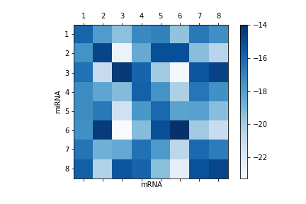
Figure 6: Logarithms of the averages, computed across all blocks, of the entries of the matrix derived from the optimal transport matrix $\tilde{P}$ during step 2 of algorithm WTOT-SCC2 and after its rearrangement.

Matching.

We run the WTOT-matching algorithm with $k=k^{\prime}=10$ and $q=90\%$. For the anecdote, we observe $(\tilde{k}_{r},\tilde{k}_{c})\approx(1.82,6.04)$ (recall that $\tilde{k}_{r},\tilde{k}_{c}$ are the row- and column-specific averages of the cardinalities of the sets $\mathcal{N}_{m}$ and $\mathcal{M}_{n}$ that are not empty). We report the parameters that characterize the mapping $\widehat{\theta}$ in Appendix A.

As an illustration, the mirrored profile (the opposite value of $y_{n}$) of the Mir20b miRNA is displayed in Figure 7 along with its three matched mRNAs (Ahrr, Cnih3 and Relb) obtained by running algorithm WTOT-matching algorithm with $k=k^{\prime}=10$. Recall that the original profile of Mir20b can be found in Figure 1.

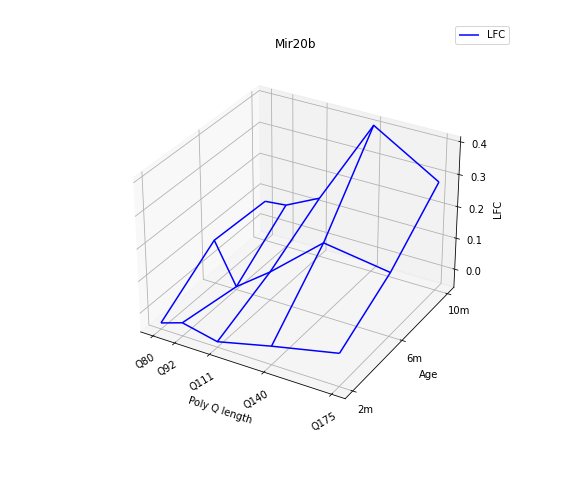
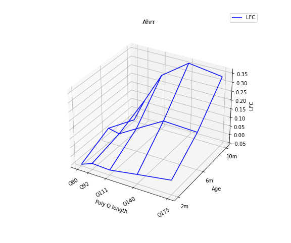
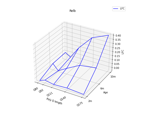
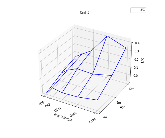
Figure 7: Minus the profile $-y_{n}$ of the Mir20b miRNA (top left), and profiles $x_{m}$ of its matched mRNAs, Ahrr (top right), Relb (bottom left) and Cnih3 (bottom right).

6.3 Biological analysis of the results

In an effort to guarantee biological relevance to the matchings, we only retain those showing evidence for binding sites as indicated in the databases TargetScan [19], MicroCosm [6] and miRDB [10]. Specifically, a pair $(x,y)$ is retained if and only if the mRNA whose profile is $x$ and the miRNA whose profile is $y$ are both among the 27,355 mRNAs and 1,478 miRNAs appearing in the TargetScan, MicroCosm and miRDB databases. The 1,247 matchings retained out of the 7,521 output by the WTOT-matching algorithm are all presented on this page of the companion website. We stress that we would have obtained fewer matchings if we had excluded from the collections $X$ and $Y$ the profiles of mRNA or miRNA which do not appear in the databases.

Furthermore, we build upon two previous analyses of miRNA regulation in the striatum of HD knock-in-mice [17, 22] to comment on the biological relevance and novelty of our findings. The first analysis [17] relies on the WGCNA algorithm, a weighted gene co-expression network analysis which yields clusters of genes whose expression profiles are correlated. The second analysis [22] relies on the MiRAMINT algorithm. MiRAMINT is a pipeline whose main steps consist in (a) carrying out a weighted gene co-expression network analysis, (b) using random forests to select candidate matchings, and (c) using Spearman’s correlation test and a multiple testing procedure to identify the more reliable matchings. We highlight that WGCNA outputs 1,583 mRNA-miRNA matchings showing evidence for binding sites in the databases TargetScan, MicroCosm and miRDB, which involve only 46 different miRNAs. As for MiRAMINT, it only outputs 31 matchings of which 20 show evidence for binding sites in the databases TargetScan, MicroCosm and miRDB, involving 14 different miRNAs. The 31 mRNA-miRNA matchings output by MiRAMINT are all presented on this webpage.

Analyzing the overlaps.

Three mRNA-miRNA matchings are retained both by the WTOT-matching and WGCNA algorithms: Mir186-Chl1, Mir132-Fam196b, Mir212-Fam196b. No matchings are retained both by the WTOT-matching and the MiRAMINT algorithms. One pair is retained both by the MiRAMINT and WGCNA algorithms: Mir132-Pafah121.

Figure 8 in Appendix A presents two Venn diagrams summarizing the overlaps between the sets of miRNAs (respectively, mRNAs) which belong to a pair output by the WGCNA, MiRAMINT and WTOT-matching algorithms. On the one hand, focusing on miRNAs, $13/14$ (respectively, $29/46$) miRNAs involved in a mRNA-miRNA pair output by MiRAMINT (respectively, WGCNA) are among the miRNAs involved in a mRNA-miRNA pair output by WTOT-matching. On the other hand, focusing on mRNAs, $1/20$ (respectively, $100/1,583$) miRNAs involved in a mRNA-miRNA pair output by MiRAMINT (respectively, WGCNA) are among the miRNAs involved in a mRNA-miRNA pair output by WTOT-matching. We carry out one-sided Fisher’s exact tests to quantify to what extent the overlaps reflect an agreement between two algorithms (using the 1,478 miRNAs and 27,355 mRNAs appearing in the TargetScan, MicroCosm and miRDB databases as reference populations). The $p$-value of the test comparing WTOT-matching and MiRAMINT equals 0.45. The other $p$-values are smaller than $10^{-6}$.

It is desirable to identify miRNAs that are particularly susceptible to play a distinct role in HD in mice. To do so, we evaluate two simple criteria on the mRNAs associated to each miRNA (the miRNAs with no matched mRNAs are obviously less interesting in our study). The criteria assess to what extent a mRNA profile is “monotonic” and, on the contrary, to what extent it is “peaked”, accounting for the amplitude of log-fold change. Formally, rewriting each profile $x\in\mathbb{R}^{15}$ as a matrix $(\tilde{x}_{tq})_{t\in\llbracket 3\rrbracket,q\in\llbracket 5\rrbracket}$, the first criterion is the minimum (relative to time $t$) of the absolute values of the slopes of the regression lines of the sets $\{(q,\tilde{x}_{tq}):q\in\llbracket 5\rrbracket\}$ and the second criterion is $\max_{q\in\llbracket 5\rrbracket}(\tilde{x}_{1q}-\tilde{x}_{2q})\times(\tilde{x}_{2q}-\tilde{x}_{3q})$. By convention, a miRNA profile is labeled monotonic (respectively, peaked) if at least one of its associated mRNA profiles is such that its first (respectively, second) criterion is larger than 95% (respectively, smaller than 99%) of the similar criteria. Moreover, all mRNA profiles $x$ appearing in a pair $(x,y)$ are labeled like $y$. We stress that no mRNA labeling conflicts occur.

Below, we reproduce the same analysis as above focusing in turn on mRNA-miRNA matchings labeled as peaked, monotonic, and neither peaked nor monotonic.

Peaked profiles.

Figure 9 in Appendix A presents two Venn diagrams summarizing the overlaps between the sets of miRNAs (respectively, mRNAs) which belong to a pair output by the WGCNA, MiRAMINT and WTOT-matching algorithms, looking at the WTOT-matching matchings labeled as peaked. None of the 17 miRNAs and none of the 12 mRNAs involved in a mRNA-miRNA pair output by WTOT-matching are involved in a mRNA-miRNA pair output by the WGCNA or MiRAMINT algorithms.

The take-home message is that the WTOT-algorithm retains mRNA-miRNA matchings that we label as peaked whereas neither the WGCNA nor the MiRAMINT algorithms do.

Monotonic profiles.

Figure 10 in Appendix A presents two Venn diagrams summarizing the overlaps between the sets of miRNAs (respectively, mRNAs) which belong to a pair output by the WGCNA, MiRAMINT and WTOT-matching algorithms, looking at the WTOT-matching matchings labeled as monotonic. On the one hand, focusing on miRNAs, $8/14$ (respectively, $9/46$) miRNAs involved in a mRNA-miRNA pair output by MiRAMINT (respectively, WGCNA) are among the miRNAs involved in a mRNA-miRNA pair output by WTOT-matching. On the other hand, focusing on mRNAs, $0/20$ (respectively, $14/1,583$) miRNAs involved in a mRNA-miRNA pair output by MiRAMINT (respectively, WGCNA) are among the miRNAs involved in a mRNA-miRNA pair output by WTOT-matching. We carry out one-sided Fisher’s exact tests to quantify to what extent the overlaps reflect an agreement between two algorithms (using the 1,478 miRNAs and 27,355 mRNAs appearing in the TargetScan, MicroCosm and miRDB databases as reference populations), excluding the comparison of the MiRAMINT and WTOT-matching algorithms in mRNAs (due to an empty intersection). The $p$-values are smaller than $10^{-5}$.

The take-home message is that, in matchings that we label as monotonic, the agreement between the WTOT-matching and WGCNA algorithms is better than that between the WTOT-matching and MiRAMINT algorithms.

Neither peaked nor monotonic profiles.

Finally, Figure 11 in Appendix A presents two Venn diagrams summarizing the overlaps between the sets of miRNAs (respectively, mRNAs) which belong to a pair output by the WGCNA, MiRAMINT and WTOT-matching algorithms and labeled neither as peaked nor monotonic. On the one hand, focusing on miRNAs, $12/14$ (respectively, $28/46$) miRNAs involved in a mRNA-miRNA pair output by MiRAMINT (respectively, WGCNA) are among the miRNAs involved in a mRNA-miRNA pair output by WTOT-matching. On the other hand, focusing on mRNAs, $1/20$ (respectively, $86/1,583$) miRNAs involved in a mRNA-miRNA pair output by MiRAMINT (respectively, WGCNA) are among the miRNAs involved in a mRNA-miRNA pair output by WTOT-matching. We carry out one-sided Fisher’s exact tests to quantify to what extent the overlaps reflect an agreement between two algorithms (using the 1,478 miRNAs and 27,355 mRNAs appearing in the TargetScan, MicroCosm and miRDB databases as reference populations), excluding the comparison of the MiRAMINT and WTOT-matching algorithms in mRNAs (due to an intersection reduced to a singleton). The $p$-value are smaller than $10^{-5}$.

The take-home message is that, in matchings that we label as neither peaked nor monotonic, the agreement between the WTOT-matching and WGCNA algorithms is better than that between the WTOT-matching and MiRAMINT algorithms.

Enrichment analysis.

Next, we assess and compare the biological significance of the mRNAs retained by the WGCNA, MiRAMINT and WTOT-matching algorithms. To do so we carry out an enrichment analysis using the EnrichR tools [8, 14, 31]. We consider only top annotations (balancing a small $p$-value and a large number of hits) as provided by Gene Ontology data (biological process, cellular content) and KEGG data. When necessary, only the top 40 hits are considered so as to guarantee a sufficient level of biological precision. Pubmed searches are also used to assess the biological significance of predicted miRNA regulation.

Figures 12, 13 and 14 in Appendix A present the mRNA-miRNA networks based on the mRNA-miRNA matchings output by the WTOT-matching algorithm, focusing on the matchings which are labeled as peaked, monotonic and neither peaked nor monotonic (in that order). The mRNAs and miRNAs retained by the WGCNA and MiRAMINT algorithms are colored. The enrichment analysis reveals

• that the mRNA-miRNA matchings output by the WGCNA algorithm are primarily annotated for axonogenesis, which relates to cytoskeleton dynamics and cell morphology;

• that the matchings output by the MiRAMINT algorithm are primarily annotated for regulation of defense response to virus by host, which relates to stress response and innate immunity;

• that the matchings output by the WTOT-matching algorithm are primarily annotated for extracellular matrix organization (which relates to cell identity), due to the matchings labeled as neither peaked nor monotonic, and secondarily annotated for mitigation of host antiviral defense response, due to the matchings labeled as monotonic, and for conventional motile cilium, due to the matchings labeled as peaked.

Although the numbers of hits in some of these annotations are small, they suggest that the WTOT-matching algorithm is able to uncover a role of miRNA regulation in responding to mutant huntingtin that was not detected by the WGCNA and MiRAMINT algorithms (despite the large number of mRNAs retained by the former).

We now interpret the above results from a biological viewpoint. Recall that the peaked and monotonic profiles are especially interesting because they are more susceptible to correspond to mRNAs and miRNAs that play a distinct role in HD in mice. Extracellular matrix organization (the primary annotation of the matchings output by the WTOT-matching algorithm, driven by the mRNA-miRNA matchings labeled as neither peaked nor monotonic) is known to be regulated by miRNAs [30] and HD mutations are known to strongly affect neuronal identity via down-regulating a large number of cell identity genes [1]. Mitigation of host antiviral defense response (the first secondary annotation of the matchings output by the WTOT-matching algorithm, due to the mRNA-miRNA matchings labeled monotonic) is similar to the primary annotation of the matchings output by the MiRAMINT algorithm. Finally, conventional motile cilium (the second secondary annotation of the matchings output by the WTOT-matching algorithm, due to the mRNA-miRNA matchings labeled peaked) is a new finding.

Additionally, although miRNA levels and regulation in response to mutant huntingtin is anticipated to be dependent on cellular context and could be differentially influenced across murine models of HD, it is noticeable that the analysis of miRNA regulation in the striatum of HD knock-in mice based on the WTOT-matching algorithm retained several miRNAs that are altered in the striatum of other types of HD mice such as BACHD [24] or altered in the human HD caudate nucleus [25] such as for example Mir100, Mir127, Mir132, Mir 212 and Mir133, supporting the relevance of our findings for the study of molecular regulation in mouse and human HD.

We believe that these facts substantiate our claim that the WTOT-matching algorithm strikes a good balance between the low and high selectivity of the WGCNA and MiRAMINT algorithms. Moreover, our findings related to striatal alterations in HD mice lead to reconsidering the formerly-expressed view on a limited role of miRNA regulation in the striatum of HD mice on a systems level [22].

7 Discussion

We have developed two co-clustering algorithms (WTOT-SCC1 and WTOT-SCC2) and a matching algorithm (WTOT-matching) for the purpose of identifying groups of mRNAs and miRNAs that interact. The algorithms apply in any situation where it is of interest to cluster or match the elements of two data sets based on a parametric model $\Theta$ expressing what it means to interact for any two pair of elements from the two data sets. The algorithms rely on optimal transport, spectral co-clustering and a matching procedure. In light of [3, Section 1.3, page 25], problem-specific knowledge is injected onto two of the three main components of the transportation problem: the representation spaces (via $\Theta$) and the marginal constraints, leaving aside the cost function.

During the first stage, an optimal optimal transport plan $P$ and mapping in $\Theta$ are learned from the data using the Sinkhorn-Knopp algorithm and a mini-batch gradient descent. During the second stage, $P$ is exploited to derive either co-clusters or several sets of matched elements.

As in [22], the motivation of our study is to shed light on the interaction between mRNAs and miRNAs based on data collected in the striatum of HD model knock-in mice [16, 17]. Each data point takes the form of multi-dimensional profile. The strong biological hypothesis is that if a miRNA induces the degradation of a target mRNA or blocks its translation into proteins, or both, then the profile of the former should be similar to minus the profile of the latter — this particular form of affine relationship drives the formulation of a loosened hypothesis and definition of model $\Theta$. The fact that the algorithm learns from the data a best element in $\Theta$ provides more flexibility than in [22].

The simulation study reveals on the one hand that WTOT-SCC2 works overall better than WTOT-SCC1, but that the co-clustering task can be very challenging in the presence of many irrelevant data points (data points that do not interact). On the other hand, it shows that the performances of WTOT-matching are satisfying.

An illustration on real data is given. The results are biologically relevant and illustrate how our algorithm strikes a good balance between two moderately and highly selective, competing algorithms. Our findings lead to reconsidering the formerly-expressed view on a limited role of miRNA regulation in the striatum of HD mice on a systems level  [22].

In conclusion, there are several directions for future work. First, we will develop a similar study to better understand miRNA regulation in the cortex of HD model mice (ongoing project). Second, we will evaluate the performances of our algorithms by simulation studies based on a simulation scheme learned from the real data so as to better mimic their law (ongoing project). Third, we will put our algorithms into the general context of co-clustering and matching of datasets and carry out more benchmark tests and comparisons.

Declarations

• Funding: T. T. Y. Nguyen is funded by Université Paris Cité thanks to a Ph.D. fellowship granted by Domaine d’Intérêt Majeur Math Innov (Région Île-de-France and Fondation Sciences Mathématiques de Paris). O. Bouaziz and A. Chambaz are funded by Université Paris Cité, W. Harchaoui by Déraison.ai. C. Mendoza, L. Mégret and C. Neri are funded by the CHDI Foundation (grant no. A-14814), Sorbonne Université, CNRS and INSERM.

• Conflicts of interest/Competing interests: None.

• Availability of data and material: The omics data used in this study are publically available through the database repository Gene Expression Omnibus (GEO) and the HDinHD portal. Overlaps between the results obtained by applying the WTOT-matching algorithm and results previously obtained based on two other algorithms, and full display of biological annotations, are available on this page of the companion website.

• Code availability: The code is available here and here.

• Authors’ contributions: C. Neri, O. Bouaziz and A. Chambaz conceived the study. T. T. Y. Nguyen, O. Bouaziz and A. Chambaz developed the methodology, formally and computationally, and performed the data analysis based on insights from L. Mégret and C. Neri on how mutant huntingtin may significantly influence expression patterns across CAG repeat alleles and age points in the brain of HD mice. L. Mégret, C. Mendoza and C. Neri performed the biological analysis of the results, the comparison to other algorithms, and the data base construction. T. T. Y. Nguyen, O. Bouaziz and A. Chambaz wrote the first draft of the manuscript. All authors commented on subsequent versions. All authors read and approved the final manuscript.

• Ethics approval: Not applicable.

• Consent to participate: Not applicable.

• Consent for publication: Not applicable.

Appendix A Supplementary material

Parametric model $\Theta$.

Introduced in Section 4.1, the parametric model $\Theta$ consists of affine mappings $\theta:\mathbb{R}^{d}\to\mathbb{R}^{d}$ of the form $x\mapsto\theta_{1}x+\theta_{2}$, where $\theta_{1}$ takes its values in a subset $T_{1}$ of $\mathbb{R}^{d\times d}$ and $\theta_{2}$ takes its values in $\mathbb{R}^{d}$ (without any constraint). It is easier to describe the set of linear mappings $\{x\mapsto\theta_{1}x:\theta_{1}\in T_{1}\}$ after a reparametrization.

In the rest of this section only, we rewrite the mRNA and miRNA profiles $x,y\in\mathbb{R}^{d}$ under the form of $d_{1}\times d_{2}$ matrices $\tilde{x}=(\tilde{x}_{tq})_{t\in\llbracket d_{1}\rrbracket,q\in\llbracket d_{2}\rrbracket}$ and $\tilde{y}=(\tilde{y}_{tq})_{t\in\llbracket d_{1}\rrbracket,q\in\llbracket d_{2}\rrbracket}$. For each $t\in\llbracket d_{1}\rrbracket$ and $q\in\llbracket d_{2}\rrbracket$, $\tilde{x}_{t\bullet}$ and $\tilde{x}_{\bullet q}$ are the $t$th row and $q$th column of $\tilde{x}$. Here, indices $t$ and $q$ correspond to the age and CAG lengths of the mice whose RNA sequencing yielded $\tilde{x}_{tq}$ and $\tilde{y}_{tq}$.

The definition of $T_{1}$ should formalize what we consider to be a (plausible) mirroring relationship. The simplest mirroring relationship is $y=-x$ or, equivalently, $\tilde{y}=-\tilde{x}$. The equality is of course too stringent/rigid, and the definition of $T_{1}$ is driven by our wish to relax it.

Biological arguments encourage us to consider that $y$ and $x$ exhibit a (plausible) mirroring relationship if, for each $(t,q)$ ($t\in\llbracket d_{1}\rrbracket$, $q\in\llbracket d_{2}\rrbracket$), $\tilde{y}_{tq}$ is strongly negatively correlated with $\tilde{x}_{tq}$, mainly, and (positively or negatively) correlated with $\tilde{x}_{(t-1)q}$ (if $t>1$) and/or with $\tilde{x}_{t(q-1)}$ (if $q>1$), secondarily. We thus formalize $\{x\mapsto\theta_{1}x:\theta_{1}\in T_{1}\}$ as the set of all linear mappings of the form

$$x\mapsto\tilde{\theta}_{1}^{a}\odot\tilde{x}+\tilde{\theta}_{1}^{b}\odot\left(\begin{smallmatrix}\textbf{0}_{d_{2}}^{\top}\\ \tilde{x}_{1\bullet}\\ \vdots\\ \tilde{x}_{(d_{1}-1)\bullet}\end{smallmatrix}\right)+\tilde{\theta}_{1}^{c}\odot\left(\textbf{0}_{d_{1}}\tilde{x}_{\bullet 1}\;\cdots\tilde{x}_{\bullet(d_{2}-1)}\right)$$

where $\tilde{\theta}_{1}^{a}$ and $\tilde{\theta}_{1}^{b},\tilde{\theta}_{1}^{c}$ are $d_{1}\times d_{2}$ matrices (here, $\odot$ is the componentwise multiplication). The entries of $\tilde{\theta}_{1}^{a}$ correspond to comparisons between $\tilde{x}_{tq}$ and $\tilde{y}_{tq}$ (same poly Q length $q$ and age $t$). The entries of $\tilde{\theta}_{1}^{b}$ (whose first row consists of 0s) correspond to comparisons between $\tilde{x}_{(t-1)q}$ and $\tilde{y}_{tq}$ (same poly Q length $q$, different age $t$). The entries of $\tilde{\theta}_{1}^{c}$ (whose first column consists of 0s) correspond to comparisons between $\tilde{x}_{t(q-1)}$ and $\tilde{y}_{tq}$ (different poly Q length $q$, same age $t$).

In the simulation study presented in Section 5, the entries of $\tilde{\theta}_{1}^{a}$ are constrained to take their values in the interval $]-5,0[$ while those of $\tilde{\theta}_{1}^{b},\tilde{\theta}_{1}^{c}$ are constrained to take their values in $]-1/2,1/2[$. The initial mapping is drawn randomly by sampling the entries of $\tilde{\theta}_{1}^{a}$ independently and uniformly in $]-5,0[$ and, independently, by sampling the entries of $\tilde{\theta}_{1}^{b}$ and $\tilde{\theta}_{1}^{c}$ independently and uniformly in $]-1/2,1/2[$.

In the illustration of the WTOT-matching algorithm presented in Section 6.2, the mapping $\widehat{\theta}$ is parametrized by $\tilde{\theta}$ given by

$$\tilde{\theta}_{1}^{a}=\left(\begin{smallmatrix}-0.88&-1.47&-0.73\\ -0.59&-0.90&-0.89\\ -0.62&-0.70&-1.17\\ -0.97&-1.30&-0.95\\ -0.56&-1.16&-1.24\\ \end{smallmatrix}\right),\quad\tilde{\theta}_{1}^{b}=\left(\begin{smallmatrix}0&0&0\\ 0.13&-0.19&0.13\\ 0.17&0.09&0.13\\ 0.19&0.09&-0.00\\ 0.18&0.15&0.08\\ \end{smallmatrix}\right),$$

$$\tilde{\theta}_{1}^{c}=\left(\begin{smallmatrix}0&0.18&-0.18\\ 0&0.19&0.17\\ 0&0.04&0.15\\ 0&0.05&0.11\\ 0&0.18&0.14\\ \end{smallmatrix}\right),\quad\theta_{2}=\left(\begin{smallmatrix}-0.01&0.01&-0.00\\ 0.00&0.01&0.01\\ 0.00&0.01&0.00\\ 0.01&0.01&0.01\\ -0.01&0.01&0.01\\ \end{smallmatrix}\right)$$

(the numbers are rounded to two decimal places). We note that:

• On the one hand, the entries of $\tilde{\theta}_{1}^{a}$ are distributed around -1. On the other hand, the entries of $\theta_{2}$ are small. This is in line with the strong biological hypothesis (that is, if a miRNA induces the degradation of a target mRNA or blocks its translation into proteins, or both, then the profile of the former should be similar to minus the profile of the latter).

• The entries of $\tilde{\theta}_{1}^{b}$ and $\tilde{\theta}_{1}^{c}$ are small.

Procedure 1 Master optimal transport algorithm.

0:  $X,Y$, minibatch sizes $\widetilde{M},\widetilde{N}$, decay rate $\eta\in]0,1]$, initial regularization parameter $\gamma_{0}$, initial mapping $\theta_{0}\in\Theta$, maximal number of iterations $T$

0:  Transport coupling $\tilde{P}_{T}\in(\mathbb{R}_{+})^{M\times N}$, mapping $\theta_{T}\in\Theta$, weight $\omega_{T}$

  Compute:

• $\underline{\gamma}=\text{mean}\{\|x-x^{\prime}\|_{2}:x,x^{\prime}\in X\}$ {for entropy regularization}

• $h=\text{mean}\{\|y-y^{\prime}\|_{2}:y,y^{\prime}\in Y\}$ {for window calibration}

  Set $t\leftarrow 0$

  Set stop $\leftarrow$ FALSE

  while $\neg$ stop or $t<T$ do

     $\gamma_{t}\leftarrow\max(\gamma_{0}\times\eta^{t},\underline{\gamma})$

     Sample uniformly a minibatch of $\widetilde{M}$ observations $\tilde{x}_{1:\widetilde{M}}:=(\tilde{x}_{1},\ldots,\tilde{x}_{\widetilde{M}})$ from $X$

     Sample uniformly a minibatch of $\widetilde{N}$ observations $\tilde{y}_{1:\widetilde{N}}:=(\tilde{y}_{1},\ldots,\tilde{y}_{\widetilde{N}})$ from $Y$

     Define and compute $\theta_{t}(\tilde{x}_{1:\widetilde{M}}):=\big{(}\theta_{t}(\tilde{x}_{1}),\ldots,\theta_{t}(\tilde{x}_{\widetilde{M}})\big{)}$

     Define and compute $\omega_{t}\in(\mathbb{R}_{+})^{\widetilde{M}}$ such that $\sum_{m\in\llbracket\widetilde{M}\rrbracket}(\omega_{t})_{m}=1$ by setting

$$(\omega_{t})_{m}\propto\sum_{n\in\llbracket\widetilde{N}\rrbracket}\varphi\left(\frac{\tilde{y}_{n}-\theta_{t}(\tilde{x}_{m})}{h}\right)\quad(\text{all\;}m\in\llbracket\widetilde{M}\rrbracket)$$

where $\varphi$ is the standard normal density

     Define $\mu_{\theta_{t}(\tilde{x}_{1:\widetilde{M}})}^{\omega_{t}}$, the $\omega_{t}$-weighted empirical measure attached to $\theta_{t}(\tilde{x}_{1:\widetilde{M}})$, and $\nu_{\tilde{y}_{1:\widetilde{N}}}$, the empirical measure attached to $\tilde{y}_{1:\widetilde{N}}$

     Compute $\text{Loss}_{t}=\bar{\mathcal{W}}_{\gamma_{t}}\left(\mu^{\omega_{t}}_{\theta_{t}(\tilde{x}_{1:\widetilde{M}})},\nu_{\tilde{y}_{1:\widetilde{N}}}\right)$ and $\nabla\text{Loss}_{t}$, the gradient of $\text{Loss}_{t}$ relative to the parameter defining $\theta_{t}$ {relies on the Sinkhorn-Knopp algorithm}

     Update the parameter defining $\theta_{t}$ by performing one step of stochastic gradient descent, yielding $\theta_{t+1}$

     Check stopping criterion and update stop variable accordingly

     $t\leftarrow t+1$

  end while

  Set $\theta_{T}\leftarrow\theta_{t-1}$

  Set $\gamma_{T}\leftarrow\gamma_{t-1}$

  Define and compute $\omega_{T}\in(\mathbb{R}_{+})^{M}$ such that $\sum_{m\in\llbracket M\rrbracket}(\omega_{T})_{m}=1$ by setting

$$(\omega_{T})_{m}\propto\sum_{n\in\llbracket N\rrbracket}\varphi\left(\frac{y_{n}-\theta_{T}(x_{m})}{h}\right)\quad(\text{all\;}m\in\llbracket M\rrbracket)$$

  Compute $\tilde{P}_{T}\in\Pi(\omega_{T})$ solving $\min_{P\in\Pi(\omega_{T})}\mathcal{W}_{\gamma_{T}}\left(\mu^{\omega_{T}}_{\theta_{T}(X)},\nu_{Y}\right)$

	the WTOT(…) algorithms					the CCOT(…) algorithms
	WTOT-SCC1∗	WTOT-SCC1	WTOT-SCC2∗	WTOT-SCC2	WTOT-BC∗	CCOT-GWD	CCOT-GWB
A1	$0$	$0.068\pm 0.126$	$0$	$0.068\pm 0.126$	$0$	$0.054\pm 0.14$	$0.092\pm 0.15$
A2	$0\pm 0.001$	$0.014\pm 0.029$	$0\pm 0.001$	$0.016\pm 0.035$	$0.033\pm 0.125$	$0.105\pm 0.13$	$0.121\pm 0.146$
A3	$0.005\pm 0.005$	$0.189\pm 0.175$	$0.0182\pm 0.033$	$0.233\pm 0.179$	$0.029\pm 0.087$	$0.612\pm 0.03$	$0.532\pm 0.068$
A4	$0.326\pm 0.064$	$0.282\pm 0.232$	$0.257\pm 0.256$	$0.393\pm 0.164$	$0.05\pm 0.093$	$0.507\pm 0.123$	$0.522\pm 0.116$

Table 5: Mean ($\pm$ standard deviation) computed across the 30 independent replications of the co-clustering discrepancy obtained for configurations A1, A2, A3, A4.

	$k=k^{\prime}$	$\tilde{k}_{r}$	precision	sensitivity	specificity
A1	$10$	$7.825\pm 0.091$	$1.0\pm 0.0$	$0.118\pm 0.001$	$1.0\pm 0.0$
A1	$35$	$29.373\pm 0.261$	$1.0\pm 0.0$	$0.442\pm 0.003$	$1.0\pm 0.0$
A1	$65$	$60.649\pm 0.998$	$0.999\pm 0.002$	$0.913\pm 0.014$	$1.0\pm 0.0$
A1	$75$	$67.418\pm 0.9$	$0.981\pm 0.006$	$0.991\pm 0.013$	$0.994\pm 0.002$
A1	$95$	$76.335\pm 1.282$	$0.888\pm 0.014$	$1.0\pm 0.0$	$0.957\pm 0.005$
A1	$150$	$97.049\pm 1.182$	$0.727\pm 0.012$	$1.0\pm 0.0$	$0.879\pm 0.005$

	$k=k^{\prime}$	$\tilde{k}_{r}$	precision	sensitivity	specificity
A4	$10$	$6.964\pm 0.161$	$0.998\pm 0.003$	$0.089\pm 0.003$	$1.0\pm 0.0$
A4	$35$	$28.632\pm 0.668$	$0.995\pm 0.009$	$0.374\pm 0.01$	$1.0\pm 0.0$
A4	$65$	$54.653\pm 0.927$	$0.986\pm 0.011$	$0.668\pm 0.018$	$0.998\pm 0.002$
A4	$75$	$61.193\pm 0.724$	$0.963\pm 0.016$	$0.709\pm 0.022$	$0.993\pm 0.003$
A4	$95$	$75.856\pm 0.749$	$0.893\pm 0.017$	$0.768\pm 0.022$	$0.975\pm 0.003$
A4	$150$	$121.273\pm 3.63$	$0.783\pm 0.025$	$0.976\pm 0.023$	$0.936\pm 0.011$

Table 6: Mean ($\pm$ standard deviation) computed across the 30 independent replications of $\tilde{k}_{r}$, precision, sensitivity and specificity of the $m$-specific matchings averaged across all mRNAs for configuration A1 (left) and A4 (right).

	$k=k^{\prime}$	$\tilde{k}_{r}$	precision	sensitivity	specificity
A1	$75$	$67.418\pm 0.9$	$0.981\pm 0.006$	$0.991\pm 0.013$	$0.994\pm 0.002$
A2	$130$	$100.217\pm 2.127$	$0.976\pm 0.017$	$0.894\pm 0.027$	$0.995\pm 0.004$
A3	$120$	$82.764\pm 1.105$	$0.881\pm 0.015$	$0.902\pm 0.025$	$0.968\pm 0.004$
A4	$120$	$97.561\pm 1.836$	$0.821\pm 0.015$	$0.853\pm 0.025$	$0.95\pm 0.005$

	$k=k^{\prime}$	$\tilde{k}_{c}$	precision	sensitivity	specificity
A1	$75$	$67.418\pm 0.9$	$0.982\pm 0.006$	$0.991\pm 0.015$	$0.994\pm 0.002$
A2	$130$	$100.217\pm 2.127$	$0.984\pm 0.012$	$0.894\pm 0.028$	$0.995\pm 0.004$
A3	$120$	$110.352\pm 1.473$	$0.878\pm 0.017$	$0.9\pm 0.024$	$0.967\pm 0.004$
A4	$120$	$97.561\pm 1.836$	$0.84\pm 0.018$	$0.853\pm 0.026$	$0.951\pm 0.004$

Table 7: Mean ($\pm$ standard deviation) computed across the 30 independent replications of $\tilde{k}_{r}$ or $\tilde{k}_{c}$, precision, sensitivity and specificity of the $m$-specific matchings (left) and $n$-specific matchings (right) averaged across all mRNAs (left) and all miRNAs (right).

	the WTOT(…) algorithms					the CCOT(…) algorithms
	WTOT-SCC1∗	WTOT-SCC1	WTOT-SCC2∗	WTOT-SCC2	WTOT-BC∗	CCOT-GWD	CCOT-GWB
B1	$0.062\pm 0.151$	$0.204\pm 0.221$	$0.082\pm 0.161$	$0.204\pm 0.221$	$0.049\pm 0.125$	$0.276\pm 0.204$	$0.53\pm 0.168$
B2	$0.114\pm 0.108$	$0.418\pm 0.265$	$0.178\pm 0.207$	$0.455\pm 0.258$	$0.382\pm 0.121$	$0.477\pm 0.14$	$0.523\pm 0.115$
B3	$0.175\pm 0.086$	$0.724\pm 0.236$	$0.163\pm 0.082$	$0.775\pm 0.176$	$-$	$0.858\pm 0.042$	$0.867\pm 0.044$
B4	$0.174\pm 0.092$	$0.747\pm 0.196$	$0.171\pm 0.112$	$0.782\pm 0.159$	$-$	$0.882\pm 0.041$	$0.883\pm 0.04$

Table 8: Mean ($\pm$ standard deviation) computed across the 30 independent replications of the co-clustering discrepancy obtained for configurations B1, B2, B3, B4.

	$k=k^{\prime}$	$\tilde{k}_{r}$	precision	sensitivity	specificity
B1	$60$	$48.578\pm 5.201$	$0.885\pm 0.209$	$0.658\pm 0.191$	$0.985\pm 0.025$
B1	$80$	$63.96\pm 6.126$	$0.851\pm 0.199$	$0.816\pm 0.222$	$0.968\pm 0.03$
B1	$85$	$67.537\pm 6.193$	$0.837\pm 0.193$	$0.842\pm 0.222$	$0.961\pm 0.031$
B1	$90$	$71.214\pm 6.208$	$0.823\pm 0.186$	$0.864\pm 0.219$	$0.953\pm 0.031$
B1	$110$	$85.833\pm 6.358$	$0.753\pm 0.156$	$0.918\pm 0.202$	$0.913\pm 0.029$

	$k=k^{\prime}$	$\tilde{k}_{r}$	precision	sensitivity	specificity
B4	$10$	$6.78\pm 0.259$	$0.926\pm 0.102$	$0.321\pm 0.046$	$0.999\pm 0.001$
B4	$20$	$15.163\pm 0.619$	$0.873\pm 0.091$	$0.72\pm 0.087$	$0.996\pm 0.003$
B4	$25$	$19.033\pm 0.784$	$0.817\pm 0.084$	$0.837\pm 0.084$	$0.991\pm 0.004$
B4	$30$	$22.889\pm 0.997$	$0.754\pm 0.076$	$0.907\pm 0.077$	$0.984\pm 0.005$
B4	$40$	$31.118\pm 1.086$	$0.618\pm 0.053$	$0.969\pm 0.049$	$0.963\pm 0.005$

Table 9: Mean ($\pm$ standard deviation) computed across the 30 independent replications of $\tilde{k}_{r}$, precision, sensitivity and specificity of the $m$-specific matchings averaged across all mRNAs for configurations B1 (left) and B4 (right).

	$k=k^{\prime}$	$\tilde{k}_{r}$	precision	sensitivity	specificity
B1	$85$	$67.537\pm 6.193$	$0.837\pm 0.193$	$0.842\pm 0.222$	$0.961\pm 0.031$
B2	$60$	$48.282\pm 3.449$	$0.751\pm 0.194$	$0.838\pm 0.2$	$0.979\pm 0.022$
B3	$25$	$19.546\pm 1.151$	$0.833\pm 0.136$	$0.837\pm 0.152$	$0.992\pm 0.006$
B4	$25$	$19.033\pm 0.784$	$0.817\pm 0.084$	$0.837\pm 0.084$	$0.991\pm 0.004$

	$k=k^{\prime}$	$\tilde{k}_{c}$	precision	sensitivity	specificity
B1	$85$	$63.732\pm 8.642$	$0.844\pm 0.175$	$0.836\pm 0.229$	$0.96\pm 0.033$
B2	$60$	$44.349\pm 2.495$	$0.792\pm 0.218$	$0.819\pm 0.227$	$0.971\pm 0.024$
B3	$25$	$18.766\pm 0.97$	$0.847\pm 0.125$	$0.833\pm 0.152$	$0.991\pm 0.005$
B4	$25$	$18.833\pm 0.793$	$0.834\pm 0.087$	$0.827\pm 0.099$	$0.99\pm 0.005$

Table 10: Mean ($\pm$ standard deviation) computed across the 30 independent replications of $\tilde{k}_{r}$ or $\tilde{k}_{c}$, precision, sensitivity and specificity of the $m$-specific matchings (left) and $n$-specific matchings (right) averaged across all mRNAs (left) and all miRNAs (right).

	the WTOT(…) algorithms					the CCOT-(…) algorithms
	WTOT-SCC1∗	WTOT-SCC1	WTOT-SCC2∗	WTOT-SCC2	WTOT-BC∗	CCOT-GWD	CCOT-GWB
C1	$0.106\pm 0.1$	$0.203\pm 0.135$	$0.101\pm 0.056$	$0.194\pm 0.116$	$0.265\pm 0.255$	$0.496\pm 0.16$	$0.902\pm 0.007$
C2	$0.209\pm 0.131$	$0.252\pm 0.182$	$0.262\pm 0.141$	$0.345\pm 0.205$	$-$	$0.938\pm 0.023$	$0.971\pm 0.026$
C3	$0.609\pm 0.113$	$0.693\pm 0.154$	$0.385\pm 0.151$	$0.521\pm 0.198$	$-$	$0.926\pm 0.027$	$0.987\pm 0.002$
C4	$0.63\pm 0.141$	$0.751\pm 0.145$	$0.435\pm 0.197$	$0.6\pm 0.233$	$-$	$0.939\pm 0.027$	$0.987\pm 0.002$

Table 11: Mean ($\pm$ standard deviation) computed across the 30 independent replications of the co-clustering discrepancy obtained for configurations C1, C2, C3, C4.

	$k=k^{\prime}$	$\tilde{k}_{r}$	precision	sensitivity	specificity
C1	$10$	$7.748\pm 0.446$	$0.973\pm 0.03$	$0.156\pm 0.01$	$1.0\pm 0.0$
C1	$30$	$25.888\pm 1.418$	$0.972\pm 0.029$	$0.526\pm 0.032$	$1.0\pm 0.0$
C1	$50$	$45.521\pm 2.441$	$0.944\pm 0.025$	$0.916\pm 0.04$	$1.0\pm 0.001$
C1	$55$	$49.108\pm 3.018$	$0.93\pm 0.021$	$0.972\pm 0.025$	$0.999\pm 0.002$
C1	$60$	$51.365\pm 3.335$	$0.919\pm 0.024$	$0.993\pm 0.011$	$0.997\pm 0.004$
C1	$70$	$55.296\pm 3.312$	$0.881\pm 0.034$	$1.0\pm 0.0$	$0.985\pm 0.01$

	$k=k^{\prime}$	$\tilde{k}_{r}$	precision	sensitivity	specificity
C4	$5$	$3.293\pm 0.096$	$0.895\pm 0.023$	$0.185\pm 0.012$	$1.0\pm 0.0$
C4	$10$	$7.278\pm 0.303$	$0.899\pm 0.022$	$0.474\pm 0.029$	$1.0\pm 0.0$
C4	$15$	$11.982\pm 0.578$	$0.888\pm 0.02$	$0.787\pm 0.04$	$1.0\pm 0.0$
C4	$20$	$15.935\pm 0.864$	$0.843\pm 0.022$	$0.96\pm 0.023$	$0.997\pm 0.001$
C4	$25$	$19.138\pm 0.89$	$0.762\pm 0.032$	$0.997\pm 0.005$	$0.989\pm 0.003$
C4	$30$	$22.578\pm 1.11$	$0.671\pm 0.04$	$1.0\pm 0.0$	$0.978\pm 0.004$

Table 12: Mean ($\pm$ standard deviation) computed across the 30 independent replications of $\tilde{k}_{r}$, precision, sensitivity and specificity of the $m$-specific matchings averaged across all mRNAs for configurations C1 (left) and C4 (right).

	$k=k^{\prime}$	$\tilde{k}_{r}$	precision	sensitivity	specificity
C1	$55$	$49.108\pm 3.018$	$0.93\pm 0.021$	$0.972\pm 0.025$	$0.999\pm 0.002$
C2	$20$	$16.203\pm 0.956$	$0.955\pm 0.016$	$0.965\pm 0.021$	$0.997\pm 0.001$
C3	$20$	$15.552\pm 0.877$	$0.854\pm 0.024$	$0.968\pm 0.019$	$0.997\pm 0.001$
C4	$20$	$15.935\pm 0.864$	$0.843\pm 0.022$	$0.96\pm 0.023$	$0.997\pm 0.001$

	$k=k^{\prime}$	$\tilde{k}_{c}$	precision	sensitivity	specificity
C1	$55$	$49.056\pm 3.461$	$0.898\pm 0.06$	$0.971\pm 0.026$	$0.981\pm 0.009$
C2	$20$	$16.371\pm 0.812$	$0.953\pm 0.018$	$0.963\pm 0.023$	$0.997\pm 0.001$
C3	$20$	$15.879\pm 0.691$	$0.804\pm 0.025$	$0.969\pm 0.018$	$0.993\pm 0.001$
C4	$20$	$15.867\pm 0.635$	$0.812\pm 0.032$	$0.961\pm 0.021$	$0.993\pm 0.002$

Table 13: Mean ($\pm$ standard deviation) computed across the 30 independent replications of $\tilde{k}_{r}$ or $\tilde{k}_{c}$, precision, sensitivity and specificity of the $m$-specific matchings (left) and $n$-specific matchings (right) averaged across all mRNAs (left) and all miRNAs (right).

Figure 8: Venn diagrams summarizing the overlaps between the sets of miRNAs (left) and mRNAs (right) which belong to a pair output by the WGCNA, MiRAMINT and WTOT-matching algorithms.

Figure 9: Venn diagrams summarizing the overlaps between the sets of miRNAs (left) and mRNAs (right) which belong to a pair output by the WGCNA, MiRAMINT and WTOT-matching algorithms, focusing on the WTOT-matching matchings labeled as peaked.

Figure 10: Venn diagrams summarizing the overlaps between the sets of miRNAs (left) and mRNAs (right) which belong to a pair output by the WGCNA, MiRAMINT and WTOT-matching algorithms, focusing on the WTOT-matching matchings labeled as monotonic.

Figure 11: Venn diagrams summarizing the overlaps between the sets of miRNAs (left) and mRNAs (right) which belong to a pair output by the WGCNA, MiRAMINT and WTOT-matching algorithms, focusing on the WTOT-matching matchings which are labeled as neither peaked nor monotonic.

Figure 12: The mRNA-miRNA networks based on the mRNA-miRNA matchings output by the WTOT-matching algorithm, focusing on the matchings which are labeled as peaked. Disks correspond to miRNAs and squares to mRNAs. The top annotation is conventional motile cilium (GO:0097729, 3 hits).

Figure 13: The mRNA-miRNA networks based on the mRNA-miRNA matchings output by the WTOT-matching algorithm, focusing on the matchings which are labeled as monotonic. Disks correspond to miRNAs and squares to mRNAs. Elements also retained by the WGCNA algorithm (respectively, the MiRAMINT algorithm) are indicated in blue (respectively, yellow). The top annotation is mitigation of host antiviral defense response (GO:0050690, 2 hits).

Figure 14: The mRNA-miRNA networks based on the mRNA-miRNA matchings output by the WTOT-matching algorithm, focusing on the matchings which are labeled as neither peaked nor monotonic. Disks correspond to miRNAs and squares to mRNAs. Elements also retained by the WGCNA algorithm (respectively, the MiRAMINT algorithm) are indicated in blue (respectively, yellow). The top annotation is extracellular matrix organization (GO:0030198, 22 hits).

References

- Achour et al. [2015] M. Achour, S. Le Gras, C. Keime, F. Parmentier, F-X. Lejeune, A-L. Boutillier, C. Neri, I. Davidson, and K. Merienne. Neuronal identity genes regulated by super-enhancers are preferentially down-regulated in the striatum of Huntington’s disease mice. Human Molecular Genetics, 24(12):3481–3496, 2015.
- Ailem et al. [2016] M. Ailem, F. Role, and M. Nadif. Graph modularity maximization as an effective method for co-clustering text data. Knowledge-Based Systems, 109:160–173, 2016.
- Alvarez-Melis [2019] D. Alvarez-Melis. Optimal Transport in Structured Domains: Algorithms and Applications. PhD thesis, Massachusetts Institute of Technology, 2019.
- Baddeley and Turner [2005] A. Baddeley and R. Turner. spatstat: An R package for analyzing spatial point patterns. Journal of Statistical Software, 12(6):1–42, 2005.
- Benayoun et al. [2019] B. Benayoun, E. Pollina, P. Singh, S. Mahmoudi, I. Harel, K. Casey, B. Dulken, A. Kundaje, and A. Brunet. Remodeling of epigenome and transcriptome landscapes with aging in mice reveals widespread induction of inflammatory responses. Genome Research, 29(4):697–709, 2019.
- Betel et al. [2010] D. Betel, A. Koppal, P. Agius, C. Sander, and C. Leslie. Comprehensive modeling of microRNA targets predicts functional non-conserved and non-canonical sites. Genome Biology, 11:R90, 2010.
- Brault et al. [2014] V. Brault, C. Keribin, G. Celeux, and G. Govaert. Estimation and selection for the latent block model on categorical data. Statistics and Computing, 25:1201–1216, 2014.
- Chen et al. [2013] E. Y. Chen, C. M. Tan, Y. Kou, Q. Duan, Z. Wang, G. V. Meirelles, N. R. Clark, and A. Ma’ayan. Enrichr: interactive and collaborative html5 gene list enrichment analysis tool. BMC Bioinformatics, 14(1):1–14, 2013.
- Dhillon [2001] I. S. Dhillon. Co-clustering documents and words using bipartite spectral graph partitioning. In Proceedings of the Seventh ACM SIGKDD International Conference on Knowledge Discovery and Data Mining, KDD ’01, pages 269––274, New York, NY, USA, 2001. Association for Computing Machinery.
- Ding et al. [2016] J. Ding, X. Li, and H. Hu. TarPmiR: a new approach for microRNA target site prediction. BMC Bioinformatics, 32:2768–2775, 2016.
- Fatras et al. [2020] K. Fatras, Y. Zine, R. Flamary, R. Gribonval, and N. Courty. Learning with minibatch Wasserstein : asymptotic and gradient properties. In The 23nd International Conference on Artificial Intelligence and Statistics, volume volume 108 of PMLR, Palermo, Italy, 2020.
- Genevay et al. [2018] A. Genevay, G. Peyré, and M. Cuturi. Learning generative models with sinkhorn divergences. In Amos Storkey and Fernando Perez-Cruz, editors, Proceedings of the Twenty-First International Conference on Artificial Intelligence and Statistics, volume 84 of Proceedings of Machine Learning Research, pages 1608–1617, Playa Blanca, Lanzarote, Canary Islands, 09–11 Apr 2018. PMLR.
- Govaert and Nadif [2010] G. Govaert and M. Nadif. Model-based co-clustering for continuous data. In Machine Learning and Applications, Fourth International Conference on, pages 175–180, Los Alamitos, CA, USA, dec 2010. IEEE Computer Society.
- Kuleshov et al. [2016] M. V. Kuleshov, M. R. Jones, A. D. Rouillard, N. F. Fernandez, Q. Duan, Z. Wang, S. Koplev, S. L. Jenkins, K. M. Jagodnik, A. Lachmann, M. G. McDermott, Monteiro C. D., Gundersen G. W., and Ma’ayan A. Enrichr: a comprehensive gene set enrichment analysis web server 2016 update. Nucleic Acids Research, 44(W1):W90–W97, 2016.
- Laclau et al. [2017] C. Laclau, I. Redko, B. Matei, Y. Bennani, and V. Brault. Co-clustering through Optimal Transport. In 34th International Conference on Machine Learning, volume 70, pages 1955–1964, Sydney, Australia, August 2017.
- Langfelder et al. [2016] P. Langfelder, J. Cantle, D. Chatzopoulou, N. Wang, F. Gao, I. Al-Ramahi, X. Lu, E. Ramos, K. Merz, Y. Zhao, S. Deverasetty, A. Tebbe, C. Schaab, D. Lavery, D. Howland, S. Kwak, J. Botas, J. Aaronson, J. Rosinski, and X. Yang. Integrated genomics and proteomics define Huntingtin CAGlength–dependent networks in mice. Nature Neuroscience, 19:622–633, 02 2016.
- Langfelder et al. [2018] P. Langfelder, F. Gao, N. Wang, D. Howland, S. Kwak, T. Vogt, J. Aaronson, J. Rosinski, G. Coppola, S. Horvath, and X. Yang. MicroRNA signatures of endogenous Huntingtin CAG repeat expansion in mice. PloS One, 13(1), 2018.
- Lavancier et al. [2015] F. Lavancier, J. Møller, and E. Rubak. Determinantal point process models and statistical inference. J. R. Stat. Soc. Ser. B. Stat. Methodol., 77(4):853–877, 2015.
- Lewis et al. [2005] Benjamin P. Lewis, Christopher B. Burge, and David P. Bartel. Conserved seed pairing, often flanked by adenosines, indicates that thousands of human genes are microRNA targets. Cell, 120(1):15–20, 2005.
- Lloyd [1982] S. P. Lloyd. Least squares quantization in PCM. IEEE Transactions on Information Theory, 28:129–137, 1982.
- Maniatis et al. [2019] S. Maniatis, T. Äijö, S. Vickovic, C. Braine, K. Kang, A. Mollbrink, D. Fagegaltier, Ž. Andrusivová, S. Saarenpää, G. Saiz-Castro, M. Cuevas, A. Watters, J. Lundeberg, R. Bonneau, and H. Phatnani. Spatiotemporal dynamics of molecular pathology in amyotrophic lateral sclerosis. Science, 364(6435):89–93, 2019.
- Mégret et al. [2020] L. Mégret, S. Sasidharan Nair, J. Dancourt, J. Aaronson, J. Rosinski, and C. Neri. Combining feature selection and shape analysis uncovers precise rules for miRNA regulation in Huntington’s disease mice. BMC Bioinformatics, 21(1):75, 2020.
- Nazarov and Kreis [2021] P. V. Nazarov and S. Kreis. Integrative approaches for analysis of mRNA and microRNA high-throughput data. Computational and Structural Biotechnology Journal, 19:1154–1162, 2021.
- Olmo et al. [2021] I. G Olmo, R. P. Olmo, A. N. A. Gonçalves, R. G. W. Pires, J. T. Marques, and F. M. Ribeiro. High-throughput sequencing of BACHD mice reveals upregulation of neuroprotective miRNAs at the pre-symptomatic stage of Huntington’s disease. ASN Neuro, 13:17590914211009857, 2021.
- Petry et al. [2022] S. Petry, R. Keraudren, B. Nateghi, A. Loiselle, K. Pircs, J. Jakobsson, C. Sephton, M. Langlois, I. St-Amour, and S. S. Hébert. Widespread alterations in microRNA biogenesis in human Huntington’s disease putamen. Acta Neuropathologica Communications, 10(1):1–11, 2022.
- Peyré and Cuturi [2019] G. Peyré and M. Cuturi. Computational Optimal Transport: With Applications to Data Science. Foundations and Trends in Machine Learning Series. Now Publishers, 2019.
- Peyré et al. [2016] G. Peyré, M. Cuturi, and J. Solomon. Gromov-Wasserstein Averaging of Kernel and Distance Matrices. In ICML 2016, Proc. 33rd International Conference on Machine Learning, New-York, United States, June 2016.
- Pontes et al. [2015] B. Pontes, R. Giráldez, and J. S. Aguilar-Ruiz. Biclustering on expression data: A review. Journal of Biomedical Informatics, 57:163–180, 2015.
- R Core Team [2022] R Core Team. R: A Language and Environment for Statistical Computing. R Foundation for Statistical Computing, Vienna, Austria, 2022. URL https://www.R-project.org/.
- Rutnam et al. [2013] Z. J. Rutnam, T. N. Wight, and B. B. Yang. miRNAs regulate expression and function of extracellular matrix molecules. Matrix Biology, 32(2):74–85, 2013.
- Xie et al. [2021] Z. Xie, A. Bailey, M. Kuleshov, D. Clarke, J. Evangelista, S. Jenkins, and A. Lachmann. Gene set knowledge discovery with Enrichr. Current Protocols, 1(3):e90, 2021.
- Yang et al. [2021] H. Yang, J. Shi, and L. Carlone. TEASER: Fast and certifiable point cloud registration. IEEE Transactions on Robotics, 37(2):314–333, 2021.
- Zhao et al. [2019] J. Zhao, H. Wang, L. Dong, S. Sun, and L. Li. miRNA-20b inhibits cerebral ischemia-induced inflammation through targeting NLRP3. Int. J. Mol. Med., 43(3):1167–1178, 2019.