Tracking the vortex motion by using Brownian fluid particles

Abstract

In this paper we propose a simple yet powerful vortex method to numerically approximate the dynamics of an incompressible flow. The idea is to sample the distribution of the initial vortices of the fluid flow in question then follow vortex dynamics along Taylor’s Brownian fluid particles. The weak convergences of this approximation scheme are obtained for 2D and 3D cases, though only for small time in 3D case. Based on our method, the simulation results are quite attracting.

I Introduction

Numerical methods have become important components in the study of fluid dynamics, in particular for modeling turbulence flows. With the advance of computational power DNS (Direct Numerical Simulation), LES (Large Eddy Simulation) and other new technologies have been developed in recent years for solving the Navier-Stokes equations numerically. Among them, various vortex methods which are based on the vorticity transport equation have become an attractive approach for simulating fluid flows in particular turbulent flows. One may find a comprehensive account in the monographs Cottet and KoumoutsakosCottet and Koumoutsakos (2000), Majda and BertozziMajda and Bertozzi (2002), SaffmanSaffman (1995), Ting and KnioTing and Knio (2007), and the recent review Mimeau and MortazaviMimeau and Mortazavi (2021).

The idea of vortex methods was introduced in ChorinChorin (1973). Several vortex approximation procedures and convergence results have been established for 2D flows, see for example Anderson et al.Anderson and Greengard (1985); Beale and Majda (1982); Hald and del Prete (1978); Hald (1979, 1987) and the literature therein. For 3D vortex methods of inviscid fluid flows, the convergence with Lagrangian stretching was proved in Beale and MajdaBeale and Majda (1982). A different approach which updates the vorticity through the velocity field was proposed and the corresponding convergence result was shown in BealeBeale (1986). For viscous fluid flows, the vortex dynamics is replaced by a random dynamical system in which a Brownian motion term is added to the equation of motion of the fluid particles, and the fluid particles become Brownian fluid particles. Itô’s stochastic differential equations (SDEs) take place of ordinary differential equations (ODEs). A remarkable convergence result for 2D random vortex method has been established in Long Long (1988). For 3D viscous fluid flows however, to the best of authors’ knowledge, there is no satisfactory solution yet so far.

In the present paper, we propose a simple method of tracking the vortex dynamics of an incompressible fluid which gives surprisingly satisfactory simulations for both inviscid and viscous fluid flows. Our method is to introduce the vorticity evolution directly in terms of Brownian fluid particles specified by a set of stochastic differential equations. We do not evolve the Taylor diffusion by mollifying the Biot-Savart kernel as in the traditional vortex methods, but instead we sample the distribution of the initial vortices and develop the initial distribution according to the SDEs determined by the vorticity equation. Let us describe this approach in more detail and at the same time establish the notations we will use throughout the paper.

Let $u=(u^{1},u^{2},u^{3})$ denote the velocity of an incompressible fluid flow moving in a range without boundary constraint. Hence the velocity $u(x,t)$ satisfies the equations of motion, the Navier-Stokes equations

$$\frac{\partial}{\partial t}u^{i}+u^{j}\frac{\partial}{\partial x^{j}}u^{i}=\nu\Delta u^{i}-\frac{\partial}{\partial x^{i}}p,\quad\frac{\partial}{\partial x^{k}}u^{k}=0$$ (1)

in $\mathbb{R}^{3}$, where $i=1,2,3$, $\nu\geq 0$ is the kinetic viscosity and $p(x,t)$ is the pressure which is uniquely determined by $u(x,t)$ up to a constant at every $t$. Einstein’s convention that the term with a pair of repeated indices are summed over from 1 to 3 has been applied. The case where $\nu=0$ corresponds to inviscid fluid flows, and the Navier-Stokes equations are reduced to the Euler equations.

The vorticity of $u$ is denoted by $\omega=(\omega^{1},\omega^{2},\omega^{3})$, although, which will be specified, we will depart from this convention in order to present some results in a general setting. By definition $\omega^{i}=\varepsilon^{ijk}\frac{\partial}{\partial x^{j}}u^{k}$ for $i=1,2,3$. The vorticity equations, which are the equations of vortex motion, play a dominated role in vortex methods, and are obtained by differentiating the Navier-Stokes equations

$$\frac{\partial}{\partial t}\omega^{i}+u^{j}\frac{\partial}{\partial x^{j}}\omega^{i}=\nu\Delta\omega^{i}+\omega^{j}\frac{\partial}{\partial x^{j}}u^{i}$$ (2)

for $i=1,2,3$. The non-linear term $u\cdot\nabla\omega$ on the left-hand side is the convection of $\omega$ which appears for both 2D and 3D flows. The second non-linear term $\omega\cdot\nabla u$, representing the stretching of the vorticity, appears only in 3D flows. This fact makes substantial difference between 2D flows and 3D flows. The study of some turbulence problems (see for example SaffmanSaffman (1995), Pullin and SaffmanPullin and Saffman (1998)) can be formulated in terms of Cauchy’s initial value problem to the vorticity equations (2) together with the equation that $\omega=\nabla\wedge u$, subject to the initial vorticity $\omega_{0}=\omega(\cdot,0)$. Vortex methods aim to provide numerical schemes to the initial value problem.

The velocity $u(x,t)$, under the assumption that both $u$ and $\omega$ decay sufficiently fast at the infinity, may be recovered from reading the vorticity via the Biot-Savart law

$$u^{i}(x,t)=\int_{\mathbb{R}^{3}}\varepsilon^{ijk}G^{j}(x-y)\omega^{k}(y,t)dy$$ (3)

where $G=(G^{1},G^{2},G^{3})$ and

$$G(z)=-\frac{1}{4\pi}\frac{z}{|z|^{3}}$$

is the Biot-Savart singular integral kernel.

Now we are in a position to describe our simple random vortex dynamics. Two (random) vector fields $V(x,t)$ and $W(x,t)$ will be defined below which do not necessarily satisfy the Navier-Stokes equations nor the relation that $W=\nabla\wedge V$. Our goal is in fact to construct approximation solutions to the vorticity equation (2) directly, in the spirit which is quite like Feynman’s functional integration for Schrödinger’s equations. Hence $V$ will be the approximate velocity of $u$, and $W$ the approximation of $\omega$.

Following the general ideas in the vortex methods, we propose the following dynamics scheme for the vortex motion of an incompressible fluid flow. At the initial time $t=0$, we sample a (finite) collection of locations $x_{n}\in\mathbb{R}^{3}$, where $n$ runs through a finite index set, at which the major vortex motion may be demonstrated. For example $x_{n}$ can be the centers of vortex rings. Suppose the initial vorticity of the fluid flow is given by

$$W^{i}(x,0)=\sum_{n}A_{n}^{i}(0)\varphi(x-x_{n})$$ (4)

where $A_{n}(0)$, vectors with components $A_{n}^{i}(0)$ (for $i=1,2,3$) are the initial vortices, and $\varphi$ is a wavelet type function which should be close to the Dirac delta (at $0$) function. Hence at the initial stage, the vortices of the fluid flow are distributed among $x_{n}$ so that

$$W(x,0)\simeq\sum_{n}A_{n}(0)\delta(x-x_{n}),$$

see for example Cottet and KoumoutsakosCottet and Koumoutsakos (2000). Therefore (4) provides us with the distribution of the initial vortices in the fluid flow. The key idea is that both the loci $x_{n}$ and the initial vortices $A_{n}(0)$ are sampled so that they are representative for the vortex motion at the initial stage. The initial vorticity $W(x,0)$ will be transported along the Brownian fluid particles. More precisely the vorticity $A_{n}(0)$ at time $t>0$ is transported to a new location $X_{n}(t)$ with a new vorticity $A_{n}(t)=(A_{n}^{1}(t),A_{n}^{2}(t),A_{n}^{3}(t))$, so that the distribution of the vortices at time $t>0$ is given by

$$W^{i}(x,t)=\sum_{n}A_{n}^{i}(t)\varphi(x-X_{n}(t))$$ (5)

for $i=1,2,3$. The velocity $V(x,t)$ at time $t>0$ is defined in terms of the Biot-Savart law (3):

$$V^{i}(x,t)=\int_{\mathbb{R}^{3}}\varepsilon^{ijk}G^{j}(x-y)W^{k}(y,t)dy,$$ (6)

so that the relation between $W$ and $V$ is maintained at least partly. It remains to determine the dynamics of $A_{n}$ and $X_{n}$. By initiative, the velocity of $X_{n}=(X_{n}^{1},X_{n}^{2},X_{n}^{3})$ should be the velocity of the fluid flow, so that

$$dX_{n}^{i}(t)=V^{i}(X_{n}(t),t)dt+\sqrt{2\nu}dB^{i}(t),\quad X_{n}(0)=x_{n}$$ (7)

for $i=1,2,3$ and $B=(B^{1},B^{2},B^{3})$ is a standard 3D Brownian motion on a probability space $(\Omega,\cal{F},\mathbb{P})$. That is, $X_{n}$ are Taylor’s diffusions initiated from $x_{n}$, and therefore $X_{n}$ are the Brownian fluid particles started at $x_{n}$. The dynamics of the vortices $A_{n}=(A_{n}^{1},A_{n}^{2},A_{n}^{3})$ are determined by the following ordinary differential equations

$$dA_{n}^{j}(t)=A_{n}^{k}(t)\frac{\partial V^{j}}{\partial x^{k}}(X_{n}(t),t)dt,\quad A_{n}(0)=A_{n}(0)$$ (8)

where $i=1,2,3$, which are responsible for the vortex stretching of the fluid flow. For 2D fluid flows, since there is no vorticity stretching, so $A_{n}$ stay as constant vectors along the fluid particle trajectories, see the section about 2D flows below.

In the next section, we will translate the previous system (7), (8), (5) and (6) together into a closed system of stochastic differential equations which thus define our random vortex method.

The main contribution of the present paper is to show that the previous simple vortex dynamics gives rise to good approximations to the motions of vortex dynamics. We demonstrate this by showing several theoretical results about the approximation solutions to the vorticity equations constructed in terms of $X_{n}$ and $A_{n}$, and also by simulations based on this simple vortex method.

The paper is organized as the following. In the next Section 2, we describe the system of stochastic differential equations which implement a simple vortex method. This system of SDEs allows us to employ the Monte-Carlo simulation to the study of incompressible fluid flows, which will be demonstrated in Section 7. In Section 3, we derive the approximation vorticity equation, which takes a form of a simple stochastic partial differential equation. In Section 4 and 5 we discuss the weak convergence results with respect to certain Sobolev norms, which justify our simple vortex method. In Section 6, we discuss the 2D incompressible flows, and not surprisingly we show that weak convergence holds for all time.

II Description of the random vortex method

In this section we propose, following the approach outlined in the Introduction, a random vortex dynamics system in a slightly general setting, otherwise we will maintain the notations established in the previous section.

The main change will be made for the relation between the vorticity field $W$ and the velocity $V$ which may be not given by the vector identity $W=\nabla\wedge V$, instead it will be given in terms of a vector integral kernel $K=(K^{1},K^{2},K^{3})$, where $K^{i}$ are locally integrable functions on $\mathbb{R}^{3}$. The reason to work with a slightly general kernel $K$ than the Biot-Savart kernel $G$ is the following. For solving the initial value problem to the vorticity equations (2) where $\omega=\nabla\wedge u$ and $\textrm{div}u=0$, which are equivalent to the system (2) and (3), mathematical difficulty arises since the Biot-Savart kernel $G$ is singular, so it is natural to replace $G$ by its smooth approximations. The simple way to create an approximation is to mollify the Biot-Savart kernel $G$. That is, choosing a smooth function $\psi\geq 0$ with a compact support in $(-\frac{1}{2},\frac{1}{2})^{3}$ and $\int_{\mathbb{R}^{3}}\psi(x)dx=1$. For each $\delta>0$, set $\psi_{\delta}(x)=\delta^{-3}\psi(\delta^{-1}x)$ and $G_{\delta}(x)=G\star\psi_{\delta}(x)$, where $\star$ denotes the convolution, i.e.

$$G_{\delta}(x)=\int_{\mathbb{R}^{3}}G(y)\psi_{\delta}(x-y)dy.$$ (9)

Then $G_{\delta}$ is smooth and

$$\left\|D^{k}G_{\delta}\right\|\leq C_{k}\frac{1}{\delta^{2+k}}$$ (10)

for some constant $C_{k}>0$, for $k=1,2,\cdots$, depending only on the regularization $\psi$. Moreover $G_{\delta}\rightarrow G$ as $\delta\downarrow 0$ in distribution sense. Therefore the initial value problem to the following system

$$\frac{\partial}{\partial t}\omega^{i}+u^{j}\frac{\partial}{\partial x^{j}}\omega^{i}=\nu\Delta\omega^{i}+\omega^{j}\frac{\partial}{\partial x^{j}}u^{i}$$ (11)

with the initial data $\omega(x,0)=\omega_{0}(x)$, and

$$u^{i}(x,t)=\int_{\mathbb{R}^{3}}\varepsilon^{ijk}G_{\delta}^{j}(x-y)\omega^{k}(y,t)dy$$ (12)

for $\delta>0$ gives rise to approximation solutions, denoted by $\omega^{\delta}$ and $u^{\delta}$. In fact as long as the initial data $\omega_{0}$ is smooth with a compact support, then $\omega^{\delta}\rightarrow\omega$ as $\delta\downarrow 0$ with respect to some Sobolev norm at least for small time. Therefore, from the computational view-point, we only need to develop numerical schemes for the approximation solutions $\omega^{\delta}$ and $u^{\delta}$, thus it is important to work with singular kernels $K$ such as $G_{\delta}$. While we would like to point out that the procedure for going to the approximation equations (11) and (12) seems unnecessary for implementing the random vortex method below, rather than for the technical reason that a priori estimates are not available for 3D Navier-Stokes equations, see Lemma 1 below.

Let us now define the random vortex system. In defining the distribution of the initial vortices (4) the wavelet type function $\varphi$ is assumed to be smooth with a compact support about the original $0$. Let us assume that the support of $\varphi\geq 0$ lies inside the ball at $0$ with radius $r_{\varphi}>0$ which will be chosen to be small, and the total mass $\int_{\mathbb{R}^{3}}\varphi(x)dx=1$. These are the structure data for our random vortex scheme, which are fixed if we are not care about the convergence issue.

Let $W(x,0)$ and $W(x,t)$ (for $t>0$) be given by (4) and (5) respectively, where $x_{n}$ and $A_{n}(0)$ are sampled initially, so they are the fixed data too. We then define the vector field $V(x,t)$ by the convolution (together with the wedge product)

$$V^{i}(x,t)=\int_{\mathbb{R}^{3}}\varepsilon^{ijk}K^{j}(x-y)W^{k}(y,t)dy$$ (13)

which coincides with (3) if $K$ is the Biot-Savart kernel $G$. The dynamics of $(X_{n},A_{n})$ are still defined by (7) and (8). Together with (5) we deduce that

$$V^{i}(x,t)=-\sum_{n}\varepsilon^{ikj}A_{n}^{k}(t)K_{\varphi}^{j}(x-X_{n}(t))$$ (14)

for $i=1,2,3$, $t\geq 0$ and $x\in\mathbb{R}^{3}$, where

$$K_{\varphi}^{j}(x)=\int_{\mathbb{R}^{3}}K^{j}(x-y)\varphi(y)dy$$

(where $j=1,2,3$) turns out to be the mollification of $K^{j}$ by $\varphi$. This is a nice feature in this scheme. By utilizing equation (14) and substituting it into (7) the dynamic system for the Brownian fluid particles $X_{n}$ can be reformulated as the following SDEs

$$dX_{n}^{i}(t)=-\sum_{m}\varepsilon^{ikj}A_{m}^{k}(t)K_{\varphi}^{j}(X_{n}(t)-X_{m}(t))dt+\sqrt{2\nu}dB^{i}(t),$$

$$X_{n}(0)=x_{n},$$ (15)

and similarly the dynamics system (8) for $A_{n}$ may be written as the following ODEs

$$dA_{n}^{i}(t)=A_{n}^{l}(t)\sum_{m}\varepsilon^{ijk}\frac{\partial K_{\varphi}^{j}}{\partial x^{l}}(X_{n}(t)-X_{m}(t))A_{m}^{k}(t)dt,$$

$$A_{n}(0)=A_{n}(0),$$ (16)

where $i=1,2,3$, $m$ and $n$ run through the finite range of the initial locations $x_{n}$.

The system of SDEs (15, 16) is closed and depends only on the structure data $K$ and $\varphi$. We observe that $K_{\varphi}$ is smooth if $K$ is locally integrable under our assumption on $\varphi$.

Theorem 1

Given a finite collection of loci $x_{n}\in\mathbb{R}^{3}$ and a family of initial vortices $A_{n}(0)$, there is a unique maximal strong solution $(X_{n},A_{n})$ to SDEs (15, 16) up to the explosion time $\tau>0$. The vector fields defined by

$$W^{i}(x,t)=\sum_{n}A_{n}^{i}(t)\varphi(x-X_{n}(t))$$ (17)

and

$$V^{i}(x,t)=-\sum_{n}\varepsilon^{ikj}A_{n}^{k}(t)K_{\varphi}^{j}(x-X_{n}(t))$$ (18)

are smooth in $x$ for $t<\tau$, where $i=1,2,3$. Moreover the explosion time $\tau\geq\tau_{A(0),\varphi}$, where

$$\tau_{A(0),\varphi}=\frac{1}{\left\|A(0)\right\|\left\|DK_{\varphi}\right\|_{\infty}},$$ (19)

$\left\|A\right\|=\sum_{n}|A_{n}|$ and $\left\|f\right\|_{\infty}$ denotes the $L^{\infty}$-norm of a function on $\mathbb{R}^{3}$. We note that $\tau_{A(0),\varphi}>0$ is deterministic.

Proof. The proof follows from the standard result in Itô’s theory of stochastic differential equations, see for example Theorem 2.3 on page 173 in Ikeda and WatanabeIkeda and Watanabe (1989). The coefficients in defining SDEs (15) and (16) are in general not globally Lipschitz, but nevertheless locally Lipschitz continuous. Therefore the explosion time $\tau$ may be finite, and the maximal strong solution $(X_{n},A_{n})$ is unique for a given 3D Brownian motion $B=(B^{1},B^{2},B^{3})$ on a probability space $(\varOmega,\mathcal{F},\mathbb{P})$. To derive the estimate (19), we utilize a truncation technique. For each $L>0$, let $\theta_{L}(s)$ be the cutting-off function which equals $s$ if $|s|\leq L$ and equals $L$ if $|s|>L$. The unique strong solution $(X^{L},A^{L})$ to the truncated SDEs

$$dX_{n}^{i}(t)=-\sum_{m}\varepsilon^{ikj}\theta_{L}(A_{m}^{k}(t))K_{\varphi}^{j}(X_{n}(t)-X_{m}(t))dt+\sqrt{2\nu}dB^{i}(t)$$

and

$$dA_{n}^{i}(t)=\theta_{L}(A_{n}^{l}(t))\sum_{m}\varepsilon^{ijk}\frac{\partial K_{\varphi}^{j}}{\partial x^{l}}(X_{n}(t)-X_{m}(t))\theta_{L}(A_{m}^{k}(t))dt$$

subject to the same initial data exist for all $t$ (Theorem 2.4, page 177 in Ikeda and WatanabeIkeda and Watanabe (1989)). It follows from the second equation that

$$\left\|A_{n}^{L}(t)\right\|\leq\left\|A_{n}^{L}(0)\right\|+\int_{0}^{t}\left\|A_{n}^{L}(s)\right\|\sum_{m}\left\|DK_{\varphi}\right\|_{\infty}\left\|A_{m}^{L}(s)\right\|ds,$$ (20)

by adding the inequalities where $n$ runs through the index set, to obtain that

$$\left\|A^{L}(t)\right\|\leq\left\|A(0)\right\|+\left\|DK_{\varphi}\right\|_{\infty}\int_{0}^{t}\left\|A^{L}(s)\right\|^{2}ds$$ (21)

for $t>0$. By Gronwall’s inequality

$$\left\|A^{L}(t)\right\|\leq\frac{\left\|A(0)\right\|}{1-\left\|A(0)\right\|\left\|DK_{\varphi}\right\|_{\infty}t}$$ (22)

for all $t<\tau_{A(0),\varphi}$. The estimate (19) now follows immediately by sending $L\uparrow\infty$.

Remark 1

From (22), it is clear that

$$\lVert A(t)\rVert\leq 2\lVert A(0)\rVert$$ (23)

for $t<\frac{1}{2}\tau_{A(0),\varphi}$.

By Gronwall’s inequality, it follows from (20) that

$$\left\|A_{n}(t)\right\|\leq\left\|A_{n}(0)\right\|e^{\left\|DK_{\varphi}\right\|_{\infty}\int_{0}^{t}\left\|A(s)\right\|ds}$$ (24)

for $t<\tau_{A(0),\varphi}$, and therefore, by (23)

$$\left\|A_{n}(t)\right\|\leq\left\|A_{n}(0)\right\|e^{2\left\|DK_{\varphi}\right\|_{\infty}\left\|A(0)\right\|t}$$ (25)

for $t<\frac{1}{2}\tau_{A(0),\varphi}$.

In the next section, we demonstrate that $(W,V)$ defined in Theorem 1 is an approximation solution to the vorticity equation (2) in certain sense.

III Approximating the vorticity equation

In this section, we assume that the structure data $K,\varphi$, $x_{n}$ and $A_{n}(0)$ are given as in the previous section. $(X_{n},A_{n})$ is the unique maximal solution pair to the SDEs (15) and (16), and $V(x,t)$ and $W(x,t)$ are defined in Theorem 1.

Theorem 2

For each $x\in\mathbb{R}^{3}$, $W(x,t)$ and $V(x,t)$ are continuous semi-martingales for $t\in[0,\tau_{A(0),\varphi})$, and

$$dW^{i} =\left(W^{j}\frac{\partial V^{i}}{\partial x^{j}}-V^{j}\frac{\partial W^{i}}{\partial x^{j}}+\nu\Delta W^{i}\right)dt$$

$$-\sqrt{2\nu}\frac{\partial W^{i}}{\partial x^{j}}dB^{j}(t)+\left(F^{i}+G^{i}\right)dt$$ (26)

for $t\in[0,\tau_{A(0),\varphi}]$, where the error terms

$$F^{i}(x,t)=\sum_{n}A_{n}^{i}(t)\left(V^{j}(x,t)-V^{j}(X_{n}(t),t)\right)\frac{\partial\varphi}{\partial x^{j}}(x-X_{n}(t))$$ (27)

and

$$G^{i}(x,t)=\sum_{n}A_{n}^{j}(t)\left(\frac{\partial V^{i}}{\partial x^{j}}(X_{n}(t),t)-\frac{\partial V^{i}}{\partial x^{j}}(x,t)\right)\varphi(x-X_{n}(t)).$$ (28)

Moreover, according to (18) and (17), $V=K\star W$ where the convolution is made with the wedge product of two vectors.

Proof. Since $A_{n}(x,t)$ are continuous semi-martingales with finite variations (in $t$), by applying Itô’s formula to $W^{i}$ define in (17), we have

$$dW^{i}(x,t)$$

$$= \sum_{n}\varphi(x-X_{n}(t))dA_{n}^{i}(t)-\sum_{n}A_{n}^{i}(t)\frac{\partial\varphi}{\partial x^{j}}(x-X_{n}(t))dX_{n}^{j}(t)$$

$$+ \nu\sum_{n}A_{n}^{i}(t)\Delta\varphi(x-X_{n}(t))dt.$$

Next we substitute $dX_{n}$ and $dA_{n}$ by using the SDEs (15) and (16) to obtain that

$$dW^{i}(x,t)$$

$$= \sum_{n}\sum_{m}\varepsilon^{iqk}A_{n}^{l}(t)A_{m}^{k}(t)\varphi(x-X_{n}(t))\frac{\partial K_{\varphi}^{q}}{\partial x^{l}}(X_{n}(t)-X_{m}(t))dt$$

$$+ \sum_{n}\sum_{m}\varepsilon^{jkq}A_{m}^{k}(t)A_{n}^{i}(t)K_{\varphi}^{q}(X_{n}(t)-X_{m}(t))\frac{\partial\varphi}{\partial x^{j}}(x-X_{n}(t))dt$$

$$+ \nu\sum_{n}A_{n}^{i}(t)\Delta\varphi(x-X_{n}(t))dt$$

$$- \sqrt{2\nu}\sum_{n}A_{n}^{i}(t)\frac{\partial\varphi}{\partial x^{j}}(x-X_{n}(t))dB^{j}(t).$$ (29)

On the other hand, according to the construction (17), (18) we have

$$V^{j}\frac{\partial W^{i}}{\partial x^{j}}(x,t)$$

$$= -\sum_{m}\sum_{n}\varepsilon^{jkq}A_{m}^{k}(t)A_{n}^{i}(t)K_{\varphi}^{q}(x-X_{m}(t))\frac{\partial\varphi}{\partial x^{j}}(x-X_{n}(t))$$

$$= -\sum_{m}\sum_{n}\varepsilon^{jkq}A_{m}^{k}(t)A_{n}^{i}(t)K_{\varphi}^{q}(X_{n}(t)-X_{m}(t))\frac{\partial\varphi}{\partial x^{j}}(x-X_{n}(t))$$

$$+ \sum_{n}A_{n}^{i}(t)\left(V^{j}(x,t)-V^{j}(X_{n}(t),t)\right)\frac{\partial\varphi}{\partial x^{j}}(x-X_{n}(t)),$$

$$W^{j}\frac{\partial V^{i}}{\partial x^{j}}(x,t)$$

$$= -\sum_{n}\sum_{m}\varepsilon^{ikq}A_{m}^{j}(t)A_{n}^{k}(t)\varphi(x-X_{m}(t))\frac{\partial K_{\varphi}^{q}}{\partial x^{j}}(x-X_{n}(t))$$

$$= \sum_{n}\sum_{m}\varepsilon^{iqk}A_{n}^{l}(t)A_{m}^{k}(t)\varphi(x-X_{n}(t))\frac{\partial K_{\varphi}^{q}}{\partial x^{l}}(x-X_{m}(t))$$

$$= \sum_{n}\sum_{m}\varepsilon^{iqk}A_{n}^{l}(t)A_{m}^{k}(t)\varphi(x-X_{n}(t))\frac{\partial K_{\varphi}^{q}}{\partial x^{l}}(X_{n}(t)-X_{m}(t))$$

$$- \sum_{n}A_{n}^{l}(t)\left(\frac{\partial V^{i}}{\partial x^{l}}(X_{n}(t),t)-\frac{\partial V^{i}}{\partial x^{l}}(x,t)\right)\varphi(x-X_{n}(t))$$

and

$$\Delta W^{i}(x,t)=\sum_{n}A_{n}^{i}(t)\Delta\varphi(x-X_{n}(t)).$$

Substituting these equations into (29), we obtain (26).

We next show that $W$ and $V$ are approximation solutions to the vorticity equation (2) with the initial vorticity $W(x,0)$.

Lemma 1

Suppose the support of $\varphi$ is contained in the ball centered at $0$ with radius $r_{\varphi}>0$.

1) It holds that

$$|F(x,t)|\leq 2\left\|A(t)\right\|^{2}\left\|DK_{\varphi}\right\|_{\infty}\left\|D\varphi\right\|_{\infty}r_{\varphi}$$

and

$$|G(x,t)|\leq 2\left\|A(t)\right\|^{2}\left\|D^{2}K_{\varphi}\right\|_{\infty}\left\|\varphi\right\|_{\infty}r_{\varphi}$$

for $t<\tau_{A(0),\varphi}$ and $x\in\mathbb{R}^{3}$.

2) There is a positive constant $C$ depending only on $\left\|A(0)\right\|$, $\left\|DK_{\varphi}\right\|_{\infty}$, $\left\|D^{2}K_{\varphi}\right\|_{\infty}$, $\left\|D\varphi\right\|_{\infty}$ and $\left\|\varphi\right\|_{\infty}$ such that

$$|F(x,t)|\leq Cr_{\varphi}\quad\textrm{ and }|G(x,t)|\leq Cr_{\varphi}$$

for all $t\in\left[0,\frac{1}{2}\tau_{A(0),\varphi}\right]$ and $x\in\mathbb{R}^{3}$.

Proof. By definition (18)

$$V^{i}(x,t)=-\sum_{n}\varepsilon^{ikj}A_{n}^{k}(t)K_{\varphi}^{j}(x-X_{n}(t)),$$ (30)

we have

$$|V(x,t)-V(y,t)|\leq 2\left\|A(t)\right\|\left\|DK_{\varphi}\right\||x-y|$$ (31)

and

$$|DV(x,t)-DV(y,t)|\leq 2\left\|A(t)\right\|\left\|D^{2}K_{\varphi}\right\||x-y|.$$ (32)

Therefore 1) follows immediately and 2) follows from 1) and (23).

Corollary 1

Suppose the support of the wavelet function $\varphi$ is contained in the ball centered at $0$ with radius $r_{\varphi}>0$. Let

$$U^{i}(x,t)$$

$$= W^{i}(x,t)-W^{i}(x,0)$$

$$- \int_{0}^{t}\left(W^{j}\frac{\partial V^{i}}{\partial x^{j}}V^{j}\frac{\partial W^{i}}{\partial x^{j}}+\nu\Delta W^{i}\right)(x,s)ds$$ (33)

for $i=1,2,3$ and $t<\tau_{A(0),\varphi}$ and $x\in\mathbb{R}^{3}$. Then

$$\left|\mathbb{E}\left[U^{i}(x,t)\right]\right|\leq C_{1}\tau_{A(0),\varphi}r_{\varphi}$$ (34)

for all $t\in\left[0,\frac{1}{2}\tau_{A(0),\varphi}\right]$.

Proof. By (26) we have

$$U^{i}(x,t)=-\sqrt{2\nu}\int_{0}^{t}\frac{\partial W^{i}}{\partial x^{j}}dB^{j}(s)+\int_{0}^{t}\left(F^{i}+G^{i}\right)ds.$$

Since under the assumptions on $\varphi$, $\int_{0}^{t}\frac{\partial W^{i}}{\partial x^{j}}dB^{j}(s)$ are martingales for $t\in\left[0,\frac{1}{2}\tau_{A(0),\varphi}\right]$ so that

$$\mathbb{E}\left[U^{i}(x,t)\right]=\mathbb{E}\int_{0}^{t}\left(F^{i}+G^{i}\right)ds$$

for $i=1,2,3$ and (34) follows from Lemma 1, 2).

Remark 2

If $K=G$ is the Biot-Savart kernel, then $\textrm{div}V=0$ according to the formula (18) and

$$V^{i}(x,t)=\int_{\mathbb{R}^{3}}\varepsilon^{ijk}G^{j}(x-y)W^{k}(y,t)dy$$ (35)

which implies that $\Delta V=-\nabla\wedge W$. Therefore $W=\nabla\wedge V+\nabla f$ for some scalar function $f$, and $V$ and $W$ satisfy the vorticity equation approximately in the sense stated in Corollary 1. The equation that $W=\nabla\wedge V$ may fail in general due to the fact that $W(x,0)$ may be not divergence-free. The reason why the approximation $V$ and $W$ still do the job (see the simulations below) nicely is that in practice $\varphi$ is close to an indicator function of a small ball, and therefore $W(x,t)$ is nearly divergence-free, and the relation $W\simeq\nabla\wedge V$ may be restored approximately.

IV Weak convergence

A simple procedure of sampling the initial vortices, for the sake of theoretical study, may be described as the following. Suppose $\omega_{0}$ is the initial vorticity, which is smooth with a compact support $S$, to the initial value problem to the vorticity equations (2). Let $\psi$ be described at the beginning of the previous section which defines $G_{\delta}$ for every $\delta>0$.

Lemma 2

Let $p\geq 1$, and the error terms in the random vortex scheme, $F(x,t)$ and $G(x,t)$ be defined by (27) and (28).

1) The following two estimates hold:

$$\left\|F(\cdot,t)\right\|_{W^{-1,p}}\leq 6\left\|A(t)\right\|^{2}\left(\left\|DK_{\varphi}\right\|\left\|\varphi\right\|_{L^{p}}r_{\varphi}+\left\|\varphi\nabla\wedge K_{\varphi}\right\|_{L^{p}}\right)$$ (36)

and

$$\left\|G(x,t)\right\|_{L^{p}}\leq 2\left\|A(t)\right\|^{2}\left\|D^{2}K_{\varphi}\right\|_{\infty}\left\|\varphi\right\|_{L^{p}}r_{\varphi}$$ (37)

for all $t\in[0,\frac{1}{2}\tau_{A(0),\varphi}]$, where $\left\|\cdot\right\|_{W^{s,p}}$ denote the Sobolev norms, see Adams (1975)

2) If the singular kernel $K=G_{\delta}$, where $\delta>0$, given in (9), then there are universal constant $C_{1},C_{2}$ such that

$$\left\|F(\cdot,t)\right\|_{W^{-1,p}}\leq C_{2}\frac{r_{\varphi}}{\delta^{3}}e^{C_{1}\frac{2}{\delta^{3}}\left\|A(0)\right\|}\left\|A(0)\right\|^{2}\left\|\varphi\right\|_{L^{p}}$$

and

$$\left\|G(x,t)\right\|_{L^{p}}\leq C_{2}\frac{r_{\varphi}}{\delta^{4}}e^{C_{1}\frac{2}{\delta^{3}}\left\|A(0)\right\|}\left\|A(0)\right\|^{2}\left\|\varphi\right\|_{L^{p}}$$

for $t\in\left[0,\frac{1}{2}\tau_{A(0),\varphi}\wedge 1\right]$.

Proof. It is clear that from definition

$$\left\|D^{k}K_{\varphi}\right\|_{\infty}\leq\left\|D^{k}K\right\|_{\infty}.$$

In particular, if $K=G_{\delta}$, then

$$\left\|D^{k}K_{\varphi}\right\|_{\infty}\leq C_{k}\frac{1}{\delta^{2+k}}$$

for some universal constants $C_{1},C_{2},\ldots$. Consider the linear functional $f_{i}(h)=\int_{\mathbb{R}^{3}}F^{i}(x,t)h(x)dx$ where $h$ defined on $\mathbb{R}^{3}$is smooth with a compact support, i.e. a test function. Since

$$F^{i}(x,t)=\sum_{n}A_{n}^{i}(t)\left(V^{j}(x,t)-V^{j}(X_{n}(t),t)\right)\frac{\partial\varphi}{\partial x^{j}}(x-X_{n}(t))$$ (38)

so that

$$f_{i}(h)$$

$$= -\sum_{n}A_{n}^{i}(t)\int_{\mathbb{R}^{3}}\left(V^{j}(x,t)-V^{j}(X_{n}(t),t)\right)\varphi(x-X_{n}(t))\frac{\partial h(x)}{\partial x^{j}}dx$$

$$- \int_{\mathbb{R}^{3}}\textrm{div}V(x,t)h(x)\varphi(x-X_{n}(t))\sum_{n}A_{n}^{i}(t)dx.$$

By the definition for $V$ (see (18)) one has the elementary estimate (see the proof of Lemma 1)

$$|V^{j}(x,t)-V^{j}(y,t)|\leq 2\left\|A(t)\right\|\left\|DK_{\varphi}\right\||x-y|.$$

Since

$$\textrm{div}V(x,t) =-\sum_{n}\varepsilon^{ikj}A_{n}^{k}(t)\frac{\partial}{\partial x^{i}}K_{\varphi}^{j}(x-X_{n}(t))$$

$$=\sum_{n}A_{n}^{k}(t)\nabla\wedge K_{\varphi}(x-X_{n}(t))$$

so that

$$|\textrm{div}V(x,t)|\leq\left\|A(t)\right\||\nabla\wedge K_{\varphi}(x-X_{n}(t))|.$$

By using these estimates and the assumption that the support of $\varphi$ lies in the ball centered at $0$ with radius $r_{\varphi}$, we therefore deduce that

$$\left|f_{i}(h)\right| \leq 2\left\|A(t)\right\|^{2}\left\|DK_{\varphi}\right\|r_{\varphi}\int_{\mathbb{R}^{3}}\varphi(x-X_{n}(t))|Dh(x)|dx$$

$$+\left\|A(t)\right\|^{2}\int_{\mathbb{R}^{3}}|\nabla\wedge K_{\varphi}(x-X_{n}(t))||\varphi(x-X_{n}(t))|h(x)|dx$$

$$\leq 2\left\|A(t)\right\|^{2}\left\|DK_{\varphi}\right\|\left\|\varphi\right\|_{L^{p}}r_{\varphi}\left\|Dh\right\|_{L^{q}}$$

$$+\left\|A(t)\right\|^{2}\left\|\varphi\nabla\wedge K_{\varphi}\right\|_{L^{p}}\left\|h\right\|_{L^{q}}$$

where $p\geq 1$ and $\frac{1}{p}+\frac{1}{q}=1$, for every test function $h$ and $i=1,2,3$. Therefore

$$\left\|F(\cdot,t)\right\|_{W^{-1,p}}\leq 6\left\|A(t)\right\|^{2}\left(\left\|DK_{\varphi}\right\|\left\|\varphi\right\|_{L^{p}}r_{\varphi}+\left\|\varphi\nabla\wedge K_{\varphi}\right\|_{L^{p}}\right).$$

The estimate for the error term $G^{i}$ is trivial. In fact by (28) and (32) to obtain

$$\left\|G^{i}(x,t)\right\|_{L^{p}}$$

$$\leq \left\|\sum_{n}A_{n}^{j}(t)\left(\frac{\partial V^{i}}{\partial x^{j}}(X_{n}(t),t)-\frac{\partial V^{i}}{\partial x^{j}}(x,t)\right)\varphi(x-X_{n}(t))\right\|_{L^{p}}$$

$$\leq 2\left\|A(t)\right\|^{2}\left\|D^{2}K_{\varphi}\right\|_{\infty}\left\|\varphi\right\|_{L^{p}}r_{\varphi}$$

In particular, if $K=G_{\delta}$, then $\nabla\wedge K_{\varphi}=0$, so that

$$\left\|F(\cdot,t)\right\|_{W^{-1,p}} \leq 6\left\|A(t)\right\|^{2}\left\|DK_{\varphi}\right\|\left\|\varphi\right\|_{L^{p}}r_{\varphi}$$

$$\leq 6C_{1}\frac{r_{\varphi}}{\delta^{3}}\left\|A(t)\right\|^{2}\left\|\varphi\right\|_{L^{p}}$$

and

$$\left\|G(x,t)\right\|_{L^{p}}\leq 6C_{2}\frac{r_{\varphi}}{\delta^{4}}\left\|A(t)\right\|^{2}\left\|\varphi\right\|_{L^{p}}$$

The other conclusions follow from the following estimate: if $K=G_{\delta}$, then $\left\|DK_{\varphi}\right\|\leq C_{1}\frac{1}{\delta^{3}}$, thus by estimate (25) we obtain that

$$\left\|A(t)\right\| \leq\left\|A(0)\right\|^{2}e^{2\left\|DK_{\varphi}\right\|_{\infty}\left\|A(0)\right\|t}$$

$$\leq\left\|A(0)\right\|^{2}e^{2C_{1}\frac{1}{\delta^{3}}\left\|A(0)\right\|t}$$

$$\leq\left\|A(0)\right\|^{2}e^{C_{1}\frac{1}{\delta^{3}}\left\|A(0)\right\|}$$

for all $t\in\left[0,\frac{1}{2}\tau_{A(0),\varphi}\wedge 1\right]$. We are now in a position to state a weak convergence theorem. Choose $\delta>0$ so the solutions $\omega^{\delta}$ and $u^{\delta}$ solving (11) and (12) are good approximations to the vorticity equations (2). Let $h>0$. Let $x_{n}$ where $n=(n^{1},n^{2},n^{3})\in\mathbb{Z}^{3}$ the center of the lattice (open) box $B_{n}$ with size $h$ whose lower-left corner is $hn$. Then $\omega_{0}$ may be approximated by $\sum_{n}\omega_{0}(x_{n})1_{B_{n}}$ in $L^{p}$ space for $p\geq 1$. Let $W^{h}(x,0)=\sum_{n}A_{n,h}(0)\phi_{h}(x-x_{n})$ with $A_{n,h}(0)=\omega_{0}(x_{n})h^{3}$, where $n$ runs over all $n$ such that $B_{n}\cap S\neq\textrm{\~{A}}$, and $\phi_{h}(x)=\frac{8}{h^{3}}\phi\left(\frac{2}{h}x\right)$, where $\phi\geq 0$ is chosen so that $\phi$ is an approximation of $1_{B}$ in some Sobolev space, $\phi$ is smooth with a compact support in $B$, where $B=(-1/2,1/2)^{3}$. Then

$$\left\|A_{,h}(0)\right\|=\sum_{n}|\omega_{0}(x_{n})|h^{3}\leq h|S|+\left\|\omega_{0}\right\|_{L^{1}}\leq|S|+\left\|\omega_{0}\right\|_{L^{1}}$$

which is independent of $h\in(0,1)$ and the lattice size. With this $W^{h}(x,0)$ as the initial sampling distribution, according to Corollary 1, $V^{\delta,h},W^{\delta,h}$ defined by (18) and (17) with $K=G_{\delta}$ and $W(x,0)=W^{h}(x,0)$, are approximations in mean of the vorticity equations (2) with initial vorticity $\omega_{0}$. Notice that

$$K_{\phi_{h}}^{j}(x) =\frac{8}{h^{3}}\int_{\mathbb{R}^{3}}K^{j}(y)\phi_{h}\left(\frac{2}{h}(x-y)\right)dy$$

$$=\frac{8}{h^{3}}\int_{\mathbb{R}^{3}}K^{j}(x-y)\phi_{h}\left(\frac{2}{h}y\right)dy$$

$$=\int_{|y|_{\infty}<\frac{1}{2}}K^{j}(x-\frac{h}{2}y)\phi\left(y\right)dy$$

which yields that

$$\left\|D^{k}K_{\phi_{h}}\right\|_{\infty}\leq\left\|D^{k}K\right\|_{\infty}.$$

Suppose $K=G_{\delta}$, then

$$\left\|D^{k}K_{\phi_{h}}\right\|_{\infty}\leq C_{k}\frac{1}{\delta^{2+k}}.$$

Theorem 3

Let $\delta>0$ and $h>0$. Let $\psi$, which is used to define $K=G_{\delta}$ for every $\delta>0$, and $\phi$, which is used to define the initial $W^{h}(x,0)$ for every $h>0$, be two non-negative smooth functions with supports lying inside the box $(-\frac{1}{2},\frac{1}{2})^{3}$ with $\int_{\mathbb{R}^{3}}\psi(x)dx=\int_{\mathbb{R}^{3}}\phi(x)dx=1$ as above. Let

$$U^{\delta,h}(x,t)$$

$$= W^{\delta,h}(x,t)-W^{h}(x,0)$$

$$- \int_{0}^{t}\left(W^{\delta,h}\cdot\nabla V^{\delta,h}-V^{\delta,h}\cdot\nabla W^{\delta,h}+\nu\Delta W^{\delta,h}\right)ds.$$ (39)

Then there is $T$ depending only on $|S|+\left\|\omega_{0}\right\|_{L^{1}}$ such that

$$\left\|\mathbb{E}\left[U^{\delta,h}(\cdot,t)\right]\right\|_{W^{-1,1}}\rightarrow 0$$

for all $t\in[0,T]$, as $h\downarrow 0$ for any fixed $\delta>0$.

Proof. This follows from the above estimates and Lemma 2 item 2). While from the proof we can see that the error term tends to zero as $\delta\downarrow 0$ and $h\downarrow 0$ such that $h\ll\delta^{4}e^{-C/\delta^{3}}$ (with some positive constant $C$). This means that we need to choose the lattice size $h$ much smaller than the regularization $\delta$ in order to ensure the convergence result. We should point out that this estimate is very crude due to the lack of a priori estimates for solutions to the Navier-Stokes equations. The simulations in section 7 demonstrate that the convergence rate of our vortex method is much fast even for the case where $\delta=0$, but its proof is beyond the reach of the current mathematical analysis for these partial differential equations.

V Modified random vortex dynamics

In the previous section, we have shown our random vortex system (15, 16) converges to the vorticity equations in mean, while if the viscosity $\nu>0$ is not small, then the random perturbation term, i.e. the noise part involving Brownian motion, appearing in (26) may be not small although its mean always stays zero. To make the noise as small as possible, we may split each particle into $N$ copies of the same particle and apply independent copies of Brownian motion for these particles. Hence we propose the following SDEs

$$dX_{n,a}^{i}(t) =-\sum_{m,b}\varepsilon^{ikj}A_{m,a}^{k}(t)K_{\varphi}^{j}(X_{n,a}(t)-X_{m,b}(t))dt$$

$$+\sqrt{2\nu}dB_{n,a}^{i}(t),$$

$$X_{n,a}(0) =x_{n},$$ (40)

and

$$dA_{n,a}^{i}(t)=A_{n,a}^{l}(t)\sum_{m,b}\varepsilon^{ijk}\frac{\partial K_{\varphi}^{j}}{\partial x^{l}}(X_{n,a}(t)-X_{m,b}(t))A_{m,b}^{k}(t)dt,$$

$$A_{n,a}(0)=\frac{1}{N}A_{n}(0),$$ (41)

where $a,b$ runs from $1$ up to $N$, where $N$ is a fixed natural number, and $B_{n,a}$ are independent copies of 3D Brownian motion on some probability space $(\varOmega,\mathcal{F},\mathbb{P})$. Thus we have split the distribution of the initial vortices as

$$W(x,0) =\sum_{n}A_{n}(0)\varphi(x-x_{n})$$

$$=\sum_{n,a}A_{n,a}(0)\varphi(x-x_{n})$$

and we have used independent Brownian motions for different locations to reduce the eventual noise in the approximation vorticity equation (26). $W(x,t)$ and $V(x,t)$ are still defined in terms of (18) and (17), where the only modifications one has to make are the sums over $n,a$ rather than $n$. The approximation voticity equations (26) has the same form but with different noise term:

$$dW^{i}=\left(W^{j}\frac{\partial V^{i}}{\partial x^{j}}-V^{j}\frac{\partial W^{i}}{\partial x^{j}}+\nu\Delta W^{i}\right)dt+H^{i}+\left(F^{i}+G^{i}\right)dt$$

where $i=1,2,3$ and

$$H(x,t)=-\sqrt{2\nu}\sum_{n,a}A_{n,a}(t)\cdot\nabla\varphi(x-X_{n,a}(t))dB_{n,a}(t)$$

which can be verified by using Itô’s formula too. Hence

$$\mathbb{E}\left|\int_{0}^{t}dH(x,s)\right|^{2}$$

$$= 2\nu\frac{1}{N}\sum_{n}\int_{0}^{t}|A_{n}(s)|^{2}|\nabla\varphi(x-X_{n,a}(s))|^{2}ds$$

$$\leq \frac{4\nu}{N}\left\|\nabla\varphi\right\|_{\infty}^{2}\left\|A(0)\right\|\max_{n}|A_{n}(0)|e^{2\left\|DK_{\varphi}\right\|_{\infty}\left\|A(0)\right\|t}$$

for $t\leq\frac{1}{2}\tau_{A(0),\varphi}$, which goes to zero as $N\rightarrow\infty$. The error term estimates for $F$ and $G$ remain the same which are independent of $N$. Therefore

$$\left\|\mathbb{E}\left[|U^{\delta,h}(\cdot,t)|^{2}\right]\right\|_{W^{-1,1}}\rightarrow 0$$

for all $t\in[0,T]$, as $h\downarrow 0$ for any fixed $\delta>0$.

VI 2D case

We retain the same notations as used in the previous sections, but we work with the two dimensional vorticity equation instead. 2D case is special as we have indicated – there is no non-linear stretching term in the vorticity equation. The vorticity $\omega(x,t)$ of an incompressible fluid flow with velocity $u=(u^{1},u^{2})$ can be identified with the scalar function $\frac{\partial}{\partial x^{1}}u^{2}-\frac{\partial}{\partial x^{2}}u^{1}$, and the vorticity equation

$$\frac{\partial}{\partial t}\omega+u^{j}\frac{\partial}{\partial x^{j}}\omega=\nu\Delta\omega$$ (42)

appears as a “linear” parabolic equation. Hence the initial vortices are transported along the motion of Brownian fluid particles. Since $\textrm{div}u=0$, so that

$$\Delta u^{1}=-\frac{\partial}{\partial x^{2}}\omega,\quad\Delta u^{2}=\frac{\partial}{\partial x^{1}}\omega$$ (43)

and

$$u(x,t)=\int_{\mathbb{R}^{2}}G(x-y)\omega(y,t)dy$$

where in 2D case, the Biot-Savart kernel $G(x)=\frac{1}{2\pi}(-\frac{x_{2}}{|x|^{2}},\frac{x_{1}}{|x|^{2}})$ which is singular at the original $0$. We therefore need to treat it as for the 3D case to introduce $G_{\delta}(x)=G\ast\psi_{\delta}(x)$, where $\psi_{\delta}(x)=\delta^{-2}\psi(\delta^{-1}x)$, and $\psi(x)$ is a smooth function with total integral $1$ and a compact support lying inside $(-1/2,1/2)^{2}$. Then we have $\lVert DG_{\delta}(x)\rVert\leq C\frac{1}{\delta^{2}}$, where $C$ depends only on the regularization $\psi$. We then implement the vortex method to the approximation system (42) together with the integral relation

$$u(x,t)=\int_{\mathbb{R}^{2}}G_{\delta}(x-y)\omega(y,t)dy$$ (44)

for each fixed $\delta>0$. Since $\omega(x,t)$ is scalar, so that there is a simplification when we sample the distribution of initial vortices. As for the 3D case, $(x_{n})$ is a finite collection of points in $\mathbb{R}^{2}$ and the initial vortices $A_{n}(0)$ are scalars. The dynamic equation for $A_{n}(t)$ is no longer needed as $A_{n}(t)=A_{n}(0)=A_{n}$ are independent of $t$, and the dynamic equation for $X_{n}(t)$ is reduced to the following SDE

$$dX_{n}^{i}(t)=\sum_{m}A_{m}K_{\varphi}^{i}(X_{n}(t)-X_{m}(t)))dt+\sqrt{2\nu}dB^{i}(t),$$

$$X_{n}(0)=x_{n},$$ (45)

whose coefficients are globally Lipschitz, so that it has a unique strong solution $X_{n}(t)$ defined for all $t$. Let

$$W(x,t)=\sum_{n}A_{n}\varphi(x-X_{n}(t))$$ (46)

and

$$V^{i}(x,t)=\sum_{n}A_{n}K_{\varphi}^{i}(x-X_{n}(t))$$ (47)

By using Itô’s formula one may deduce that

$$dW(x,t)$$

$$= -V(x,t)\cdot\nabla W(x,t)dt+\nu\Delta W(x,t)dt$$

$$- \sum_{n}A_{n}\nabla\varphi(x-X_{n}(t))\cdot\sqrt{2\nu}dB(t)$$

$$- \sum_{n}A_{n}\nabla\varphi(x-X_{n}(t))\cdot(V(X_{n}(t),t)-V(x,t))dt.$$

The non-martingale error term

$$F(x,t)=\sum_{n}A_{n}\nabla\varphi(x-X_{n}(t))\cdot(V(X_{n}(t),t)-V(x,t)).$$

Following the same procedure as in the proof of Lemma 2, we may deduce the following global estimates for 2D case.

Lemma 3

1) For any $p\geq 1$

$$\lVert F\rVert_{W^{-1,p}}\leq\lVert A\rVert^{2}\bigg{(}\lVert DK_{\varphi}\rVert\lVert\varphi\rVert_{L^{p}}r_{\varphi}+\lVert\varphi\text{\text{div}}K_{\varphi}\rVert_{L^{p}}\bigg{)}.$$

2) If the singular kernel $K=G_{\delta}$, where $\delta>0$, then

$$\lVert F(\cdot,t)\rVert_{W^{-1,p}}\leq C_{5}\frac{1}{\delta^{2}}\lVert A\rVert^{2}\lVert\varphi\rVert_{L^{p}}r_{\varphi}$$

for all $t>0$ where $\lVert A\rVert=\sum_{n}|A_{n}|$.

Now we state the weak convergence theorem. Let $h>0$, and let $x_{n}$ where $n=(n_{1},n_{2})\in\mathbb{Z}^{2}$ the center of the lattice box $B_{n}$ with size $h$ whose lower left corner is $hn$. Then the initial vorticity $\omega_{0}$ may be approximated by $\sum_{n}\omega_{0}(x_{n})1_{B_{n}}$ for example in an $L^{p}$-space. Let $W^{h}(x,0)=\sum_{n}A_{n,h}\varphi_{h}(x-x_{n})$ with $A_{n,h}=\omega_{0}(x_{n})h^{2}$, where $n$ runs over all $n$ such that $B_{n}\cap S\neq\tilde{A}$, and $\varphi_{h}(x)=\frac{1}{h^{2}}\phi(\frac{x}{h})$, where $\phi$ is an approximation of $1_{B}$ where $B$ is the unit square $(-1/2,1/2)^{2}$ in $L^{p}$ space for $p>1$. Then

$$\lVert A_{,h}\rVert=\sum_{n}|\omega_{0}(x_{n})|h^{2}\leq h|S|+\lVert\omega_{0}\rVert_{L^{1}}\leq|S|+\lVert\omega_{0}\rVert_{L^{1}},$$

which is independent of $h\in(0,1)$ and the lattice size. With this $W^{h}(x,0)$ as the initial sampling distribution, let $V^{\delta,h},W^{\delta,h}$ be defined as in equations (47) and (46) with $K=G_{\delta}$. Therefore, by Lemma 3, item 2), we have the following theorem:

Theorem 4

Let

$$U^{\delta,h}(x,t) =W^{\delta,h}(x,t)-W^{h}(x,0)$$

$$-\int_{0}^{t}\left(-V^{\delta,h}\cdot\nabla W^{\delta,h}+\nu\Delta W^{\delta,h}\right)ds.$$ (48)

Then

$$\left\|\mathbb{E}\left[U^{\delta,h}(\cdot,t)\right]\right\|_{W^{-1,1}}\rightarrow 0$$

for all $t>0$ as long as $h\ll\delta^{2}$, and for any $T>0$, this convergence is uniform for all $(x,t)\in\mathbb{R}^{2}\times(0,T]$.

VII Simulation results

First we show some figures of the velocity field by our approximation scheme for 3D flows, which illustrates the velocity field projected at the plane $z=0$. The flow starts with two points at $(-1,0,0)$ and $(1,1,0)$ with vorticity $(0,0,10)$ and $(10,10,10)$ respectively. i.e $x_{1}=(-1,0,0),x_{2}=(1,1,0)$, $,A_{1}(0)=(0,0,10),A_{2}(0)=(10,10,10)$. Throughout the simulation in 3D flows, We choose the Biot-Savart kernel $G$, and we let $\varphi$ be $c(|x|^{2}-1)^{2}$, where $c$ is a constant such that the total integral of $\varphi=1$ (We find a polynomial helps improve the computational speed of numerical integration in the packages we used in program). We let $h=0.5$. Figure. 1 shows the case when $\nu=0$.

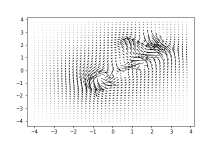
(a) $t=0$

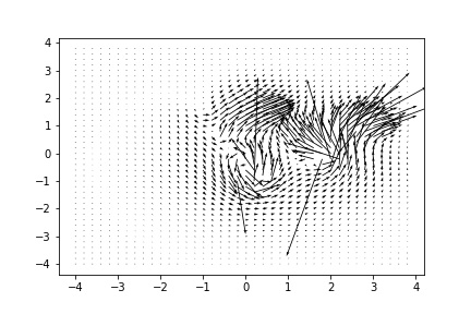
(b) $t=1$

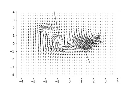
(c) $t=3$

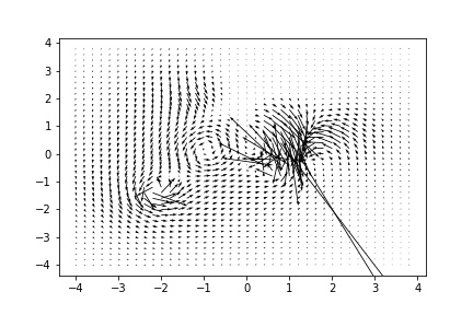
(d) $t=5$

Figure 1: An inviscid Flow

(a)

(b)

(c)

(d)

Figure 2: Split each particle into $5$ parts

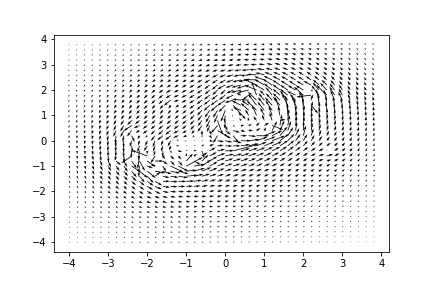
(a)

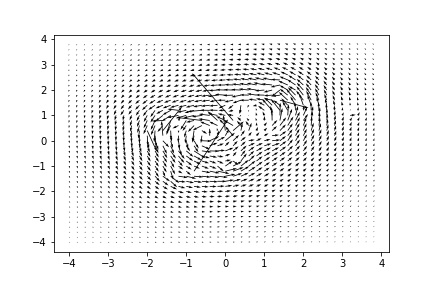
(b)

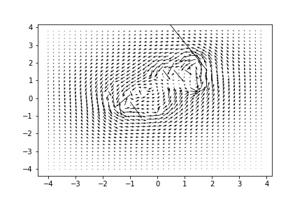
(c)

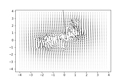
(d)

Figure 3: Split each particle into $50$ parts

When $\nu\neq 0$, we are going to split the particles as in the previous section, and we will see that more splitting helps minimise the stochastic error. We keep the choice of the kernel, $\varphi$, $h$, the initial condition as in the inviscid flow. The only difference here is that we consider the viscosity $\nu=1$ in this case, which means we have to solve a system of SDEs with the appropriate noise. We are looking at the projection of velocity field when $t=0.5$. (Figure. 2 and Figure. 3). When we split each particle into $50$ parts, the result from different randomisation is more consistent.

For 2D flows simulation, we use the 2D Biot-Savart kernel $H$, and $\varphi=c(|x|^{2}-1)^{2}$, $h=0.5$. we start the flow with randomized $(x_{n},A_{n})$ $n=1,2,\dots,10$. $x_{n}$ are sampled in $[-1,1]\times[-1,1]$ by uniform distribution independently, and $A_{n}$ are sampled in $[-10,-10]$ by uniform distribution. The particles inside the flow are denoted by different colors, and then we look at their locations at different time. (Figure. 4)

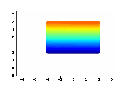
(a) $t=0$

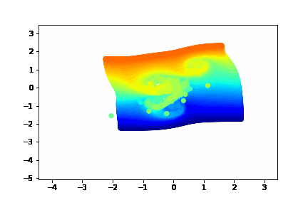
(b) $t=0.3$

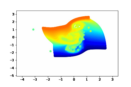
(c) $t=0.6$

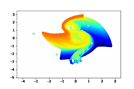
(d) $t=1$

Figure 4: The dynamics of an inviscid flow

Figure. 5 is the vorticity picture for a non-inviscid flow with viscosity $\nu=1$. We use the same kernel, $\varphi$, $h$ as in the previous simulation. We let $(x_{1},x_{2},x_{3},x_{4})$ be sampled in $\mathbb{R}^{2}$ by $N(0,I)$, with vorticity $(10,10,-10,-10)$ respectively. We split each particle into $50$ parts to minimise the stochastic error. The vorticity value at each point is represented by its color, and the relations between the color and vorticity are shown in the bar on the right of each figure. The blue color represents positive vorticity, and the red color represents negative vorticity.

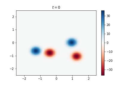
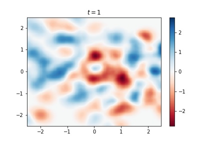
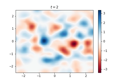
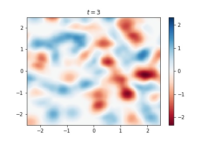
Figure 5: Vorticity of a non-inviscid flow

Data Availability Statement

The data that support the findings of this study are available from the corresponding author upon reasonable request.

References

Cottet and Koumoutsakos (2000)G. H. Cottet and P. D. Koumoutsakos, Vortex methods:
theory and practice (Cambridge University Press, 2000).
Majda and Bertozzi (2002)A. J. Majda and A. L. Bertozzi, Vorticity and
incompressible flow (Cambridge University Press, 2002).
Saffman (1995)P. G. Saffman, Vortex dynamics (Cambridge University Press, 1995).
Ting and Knio (2007)R. Ting, L.; Klein and O. M. Knio, Vortex dominated flows: analysis and computation for multiple scale
phenomena (Springer-verlag, 2007).
Mimeau and Mortazavi (2021)C. Mimeau and I. Mortazavi, “A review of
vortex methods and their applications: from creation to recent advances,” Fluids 6, 68 (2021).
Chorin (1973)A. J. Chorin, “Numerical study
of slightly viscous flow,” J. Fluid Mech 57, 785–796 (1973).
Anderson and Greengard (1985)C. Anderson and C. Greengard, “On vortex
methods,” SIAM
J. Numer. Anal. 22, 413–440 (1985).
Beale and Majda (1982)J. T. Beale and A. Majda, “Vortex methods. i.
convergence in three dimensions,” Mathematics of Computation 39, 1–27 (1982).
Hald and del
Prete (1978)O. Hald and V. M. del
Prete, “Convergence of
vortex methods for euler’s equations,” Mathematics of Computation 32, 791–809 (1978).
Hald (1979)O. Hald, “Convergence of
vortex methods for euler’s equations, ii,” SIAM Journal on Numerical Analysis 16, 726–755 (1979).
Hald (1987)O. Hald, “Convergence of
vortex methods for euler’s equations, iii,” SIAM Journal on Numerical Analysis 24, 538–582 (1987).
Beale (1986)J. T. Beale, “A convergent 3-d
vortex method with grid-free stretching,” Mathematics of Computation 46, 401–424 (1986).
Long (1988)D. G. Long, “Convergence of the
random vortex method in two dimensions.” Journal of the American Mathematical
Society 1, 779–804
(1988).
Pullin and Saffman (1998)D. I. Pullin and P. G. Saffman, “Vortex dynamics
in turbulence,” Annu. Rev. Fluid Mech. 30, 31–51 (1998).
Ikeda and Watanabe (1989)N. Ikeda and S. Watanabe, Stochastic
differential equations and diffusion processes, 2nd ed. (North-Holland Publishing Company, 1989).
Adams (1975)R. A. Adams, Sobolev spaces (Academic Press, 1975).