Technical Report: Distributed Sampling-based Planning for
Non-Myopic Active Information Gathering

Abstract

This paper addresses the problem of active information gathering for multi-robot systems. Specifically, we consider scenarios where robots are tasked with reducing uncertainty of dynamical hidden states evolving in complex environments. The majority of existing information gathering approaches are centralized and, therefore, they cannot be applied to distributed robot teams where communication to a central user is not available. To address this challenge, we propose a novel distributed sampling-based planning algorithm that can significantly increase robot and target scalability while decreasing computational cost. In our non-myopic approach, all robots build in parallel local trees exploring the information space and their corresponding motion space. As the robots construct their respective local trees, they communicate with their neighbors to exchange and aggregate their local beliefs about the hidden state through a distributed Kalman filter. We show that the proposed algorithm is probabilistically complete and asymptotically optimal. We provide extensive simulation results that demonstrate the scalability of the proposed algorithm and that it can address large-scale, multi-robot information gathering tasks, that are computationally challenging for centralized methods.

I INTRODUCTION

Recent advances in sensing and perception have enabled the deployment of mobile robots in unknown environments for information gathering missions such as environmental monitoring [1], [2], surveillance [3], coverage [4], [5], target tracking [6],[7] and active-SLAM [8], [9]. These tasks require spatio-temporal information collection, which can be achieved more efficiently by multi-robot systems, rather than relying on individual robots. To avoid the need for a central user computing sensor-based control policies for large multi-robot systems, distributed control frameworks are needed allowing robots to make decisions locally.

In this paper, we are interested in designing distributed control policies for a team of mobile sensing robots tasked with actively reducing the accumulated uncertainty of a dynamic hidden state over an a priori unknown horizon while satisfying user-specified accuracy requirements. In particular, first we formulate the Active Information Acquisition (AIA) problem as a stochastic optimal control problem. Then, building upon the separation principle presented in [10], we convert the stochastic optimal control problem into a deterministic optimal control problem via the use of a Distributed Kalman Filter (DKF) for which offline/open-loop control policies are optimal. To solve the resulting deterministic optimal control problem, we propose a novel distributed sampling-based method under which all robot incrementally and in parallel build their own directed trees that explore both their respective robot motion and information space. To build these trees, the robots communicate with each other over an underlying connected communication network to exchange their beliefs about the hidden state which are then fused using a DKF [11]. We show that the proposed algorithm is probabilistically complete and asymptotically optimal. The proposed scheme is evaluated through extensive simulations for a target localization and tracking scenario.

Literature Review: Relevant works that address informative planning problems can be categorized into myopic/greedy and non-myopic (sampling-based and search-based). Myopic approaches typically rely on gradient-based controllers that although they enjoy computational efficiency, they suffer from local optima [12, 13, 14, 15, 16, 17, 18]. In [15] a decentralized, myopic approach is introduced where the robots are driven along the gradient of the Mutual Information (MI) between the targets and the sensor observations. To mitigate the issue of local optimality, non-myopic search-based approaches have been proposed that can design optimal paths [19]. Typically, these methods are computationally expensive as they require exploring exhaustively both the robot motion and the information space in a centralized fashion. More computationally efficient but suboptimal controllers have also been proposed that rely on pruning the exploration process and on addressing the information gathering problem in a decentralized way via coordinate descent [20, 9, 21]. However, these approaches become computationally intractable as the planning horizon or the number of robots increases as decisions are made locally but sequentially across the robots. Monte Carlo Tree Search [22] has recently gain popularity for online planning in robotics. Best et. al [23] suggest the Dec-MCTS algorithm that efficiently samples the individual action space of each robot on contrary to our proposed method and then coordinates with a sparse approximation of the joint action space. To do so, the robots must exchange branches of their Monte-Carlo trees, burdening further the communication needs. Nonmyopic sampling-based approaches have also been proposed due to their ability to find feasible solutions very fast, see e.g., [24, 25, 26, 27]. Common in these works is that they are centralized and, therefore, as the number of robots or the dimensions of the hidden states increase, the state-space that needs to be explored grows exponentially and, as result, sampling-based approaches also fail to compute sensor policies because of either excessive runtime or memory requirements. A more scalable but centralized sampling-based approach is proposed in [28] that requires communication to a central user for both estimation and control purposes. Building upon our previous work [28], we propose a novel distributed sampling-based algorithm that scales well with the number of robots and planning horizon while allowing the robots to locally and simultaneously explore their physical and reachable information space, exchange their beliefs over an underlying communication network, and fuse them via a DKF.

Contributions: The contribution of this paper can be summarized as follows. First, we propose a distributed nonmyopic sampling-based approach for information-gathering tasks. Second, we propose the first distributed sampling-based information gathering algorithm that is probabilistically complete and asymptotically optimal, while it signfinicantly decreases the computational complexity per iteration of its centralized counterpart [28]. Third, we provide extensive simulation results that show that the proposed method can efficiently handle large-scale estimation tasks.

II Problem Formulation

II-A Robot Dynamics, Hidden State, and Observation Model

Consider a team of $N$ mobile robots that reside in a complex environment $\Omega\subset\mathbb{R}^{d}$ where $d$ is the dimension of the workspace. Obstacles of arbitrary shape are denoted as $\mathcal{O}$ and the obstacle-free area is $\Omega_{\text{free}}\coloneqq\Omega\backslash\mathcal{O}.$ The dynamics of the robots are governed by the following equation

$$\mathbf{p}_{i}(t+1)=f_{i}(\mathbf{p}_{i}(t),\mathbf{u}_{i}(t)),\quad i=\{1,\dots,N\}$$ (1)

where $\mathbf{p}_{i}(t)\in\Omega_{\text{free}}$ describes the state of robot $i$ at discrete time $t$ (e.g position), $\mathbf{u}_{i}(t)\in\mathcal{U}_{i}$ is the control input applied to robot $i$ at time $t$ from a finite space $\mathcal{U}_{i}$ of admissible control inputs. The task of the robots is to collaboratively estimate a hidden state $\mathbf{x}(t)$ evolving in $\Omega_{\text{free}}$ governed by the following dynamics

$$\mathbf{x}(t+1)=A\mathbf{x}(t)+\mathbf{w}(t), \quad\mathbf{w}(t)\sim\mathcal{N}(\mathbf{d}(t),{\bf{Q}}(t))$$ (2)

where $\mathbf{x}(t)\in\mathbb{R}^{d_{x}}$ and $\mathbf{w}(t)\in\mathbb{R}^{d_{{w}}}$ denote the hidden states and the process noise at time $t$, respectively. Robots are equipped with sensors (e.g., cameras) which allow them to take measurements associated with the unknown state $\mathbf{x}(t)$. Hereafter, we assume that the robots can generate measurements as per the following observation model

$$\mathbf{y}_{i}(t)=M_{i}(\mathbf{p}_{i}(t))\mathbf{x}(t)+\mathbf{v}_{i}(t)$$ (3)

where $\mathbf{y}_{i}(t)$ is the measurement signal at time $t$ and $\mathbf{v}_{i}(t)\sim\mathcal{N}(\mathbf{0},\mathbf{R}_{i}(t))$ is a sensor-state dependent measurement noise. Signals observed by robot $i$ are independent of other robots’ observations.

Assumption 1

The dynamics of the state $\mathbf{x}(t)$ in (2), the control input $\mathbf{d}(t)$ the observation model (3), and process and measurement noise covariances $Q(t)$ and $R_{i}(t)$ are known for all time instants $t$. This assumption is common in the literature [10], [11] and it is required for the application of a Kalman filter to estimate the hidden states.

II-B Distributed Kalman Filter for State Estimation

Given a Gaussian prior distribution for $\mathbf{x}(0)$, i.e., $\mathbf{x}(0)\sim\mathcal{N}(\bm{\mu}(0),\Sigma(0))$, and measurements, denoted by $\mathbf{y}_{i,0:t}$, that robot $i$ has collected until a time instant $t$, robot $i$ computes a Gaussian distribution that the hidden state follows at time $t$, denoted by $\hat{\mathbf{x}}_{i}(t)=\mathcal{N}(\bm{\mu}_{i}(t|\mathbf{y}_{i,0:t}),\Sigma_{i}(t|\mathbf{y}_{i,0:t}))$, where $\bm{\mu}_{i}(t|\mathbf{y}_{i,0:t})$ and $\Sigma_{i}(t|\mathbf{y}_{i,0:t})$ denote the a-posteriori mean and covariance matrix. To compute this local Gaussian distribution, we adopt the Distributed Kalman Filter (DKF) algorithm proposed in [11]. To this end, we assume that the robots formulate an underlying communication network modeled as an undirected graph $G=(V,E)$. The sets $V$ and $E$ denote the set of vertices, defined as $V\coloneqq\{1,\dots,N\}$ and indexed by the robots, and set of edges where existence of an edge $(i,j)$ means that robots $i$ and $j$ can directly communicate with each other. Given, such a communication graph, every robot $i$ updates its respective Gaussian distribution as follows:

$$\Omega_{i}(t+1)=\sum\limits_{j\in\mathcal{N}_{i}\cup\{i\}}\kappa_{ij}\Omega_{j}(t)+M_{i}(t)^{T}R_{i}(t)^{-1}M_{i}(t)$$ (4)

where $\Omega_{i}(t)=\Sigma_{i}(t)^{-1}$, $\mathcal{N}_{i}$ is the set of nodes (neighbors) connected to robot $i$, $\kappa_{ij}>0,\sum_{j\in\mathcal{N}_{i}\cup\{i\}}\kappa_{ij}=1$.

II-C Active Information Acquisition

The quality of measurements taken by robot $i$ up to a time instant $t$, $\mathbf{y}_{i,0:t}$, can be evaluated using information measures, such as the mutual information between $\mathbf{y}_{i,0:t}$ and $\mathbf{x}(t)$ or the conditional entropy of $\mathbf{x}(t)$ given $\mathbf{y}_{i,0:t}$. Given initial robot states $\mathbf{p}_{i}(0)\in\Omega_{\text{free}}$ and a prior distribution of the hidden states $\mathbf{x}(0)$, our goal is to compute a sequence of control policies $\bm{\pi}_{i}(t)\colon\{\mathbf{u}_{i,0:t-1},\mathbf{y}_{i,0:t}\}\rightarrow\mathbf{u}_{i}(t)\in\mathcal{U}_{i}$ and a planning horizon $F$, for all robots $i\in\{1,\dots,N\}$ and time instants $t=\{0,\dots,F\}$ which solves the following stochastic optimal control problem:

$$\min\limits_{F}\max\limits_{\bm{\pi}_{0:F}}\left[J(F,\bm{\pi}_{0:F})=\sum_{i=1}^{N}\sum_{t=0}^{F}\mathbb{I}(\mathbf{x}(t+1);\mathbf{y}_{i,{0:t}})\right]$$ (5a)

$$\ \ \ \ \ \ \mathbb{I}(\mathbf{x}(F+1);\mathbf{y}_{i,0:F})\geq\epsilon\textit{ for at least one robot},$$ (5b)

$$\ \ \ \ \ \ \mathbf{p}_{i}(t+1)=f_{i}(\mathbf{p}_{i}(t),\bm{\pi}_{i}(t)),$$ (5c)

$$\ \ \ \ \ \ \mathbf{p}_{i}(t+1)\in\Omega_{\text{free}}^{N},$$ (5d)

$$\ \ \ \ \ \ \mathbf{y}_{i}(t)=M_{i}(\mathbf{p}_{i}(t))\mathbf{x}(t)+\mathbf{v}_{i}(t),$$ (5e)

$$\ \ \ \ \ \ \mathbf{x}(t+1)=A\mathbf{x}(t)+\mathbf{w}(t)$$ (5f)

where the objective in (5a) captures the accumulated mutual information between the measurements received up to time $t$ and the state $\mathbf{x}(t+1)$ of all robots and $\bm{\pi}_{0:F}$ stands for the concatenated sequence of control inputs applied to the robots from $t=0$ until $t=F$. The constraint in (5b) requires that at the end of the planning there exists at least one robot that has a comprehensive view of the state $\mathbf{x}(F+1)$ with a certain confidence $\epsilon\geq 0$. Moreover not including constraint (5b) would result in robots to stay put, i.e $F=0$. The constraints (5c), (5e) capture the robot and sensor model, respectively, while constraint (5f) is the hidden state model. Obstacle avoidance is ensured through constraint (5d).

Active Information Problem (5) is a stochastic optimal control problem for which closed-loop policies outclass open loop ones. Nonetheless, the linear relation between measurement $\mathbf{y}_{i}(t)$ and state $\mathbf{x}(t)$ in (3) and the gaussian assumptions transform the stochastic optimal control problem (5) into a deterministic optimal control problem where open loop policies are optimal [10]. The principle is extended for our case where robots communicate with neighbors $\mathcal{N}_{i}$ according to a communication graph $G=(V,E)$ and fuse their beliefs via DKF (4) and an open-loop control sequence $\sigma=\mathbf{u}(0),\dots,\mathbf{u}(F)$ exists which is optimal in (5).

Furthermore Problem (5) can be transformed to the following deterministic control problem

$$\min_{\begin{subarray}{c}F,\bm{u}_{0:F}\end{subarray}}\left[J(F,\bm{u}_{0:F})=\sum_{i=1}^{N}\sum_{t=0}^{F}\det\Sigma_{i}(t+1|\mathbf{y}_{i,{0:t}})\right]$$ (6a)

$$\ \ \ \ \ \ \ \det\Sigma_{i}(F+1)\leq\delta(\epsilon)\textit{ for at least one robot}$$ (6b)

$$\ \ \ \ \ \ \ \ \mathbf{p}_{i}(t+1)\in\Omega_{\text{free}}^{N},$$ (6c)

$$\ \ \ \ \ \ \ \ \mathbf{p}_{i}(t+1)=f_{i}(\mathbf{p}_{i}(t),\mathbf{u}_{i}(t)),$$ (6d)

$$\ \ \ \ \ \ \ \ \Omega_{i}(t+1)=\rho(\mathbf{p}_{i}(t),\Omega_{j\in\mathcal{N}_{i}\cup\{i\}}(t)),$$ (6e)

$$\ \ \ \ \ \ \ \ \Sigma_{i}(t+1)=\Omega_{i}(t+1)^{-1}$$ (6f)

where $\rho(\cdot)$ is the DKF update rule in (4), $\bm{u}_{0:F}$ is the concatenated sequence of control inputs of all robots from $t=0$ until $t=F$ and $\delta(\epsilon)\geq 0$ is the resulting uncertainty threshold from the definition of mutual information and (5b). The robots collaboratively solve the objective (6a) with each constraint applying individually to them. Note that solving (6) requires the robots to exchange their covariance matrices over the communication network $G$ due to (6e).

III Distributed Sampling Based Active Information Acquisition

A novel distributed sampling-based method to solve (6) is proposed which is summarized in Algorithm 1. In the proposed method, each robot $i$ builds, in parallel with all other robots, a local directed tree that explores both the information space and its robot motion space while exchanging information with neighboring robots collected in $\mathcal{N}_{i}$, opposed to the global tree built in [28] resulting in decreasing the computational complexity significantly.

The proposed distributed sampling-based algorithm is presented in Algorithm 1. In what follows, we denote the tree built by robot $i$ as $\mathcal{G}_{i}=\{\mathcal{V}_{i},\mathcal{E}_{i},{J_{\mathcal{G}}}_{i}\}$, where $\mathcal{V}_{i}$ is the set of nodes and $\mathcal{E}_{i}$ denotes the set of edges. The set of nodes collects states of the form $\mathbf{q}_{i}(t)=[\mathbf{p}_{i}(t),\Sigma_{i}(t),\mathcal{S}_{i}(t)]$ where $\mathcal{S}_{i}(t)$ is a set that collects nodes $\mathbf{q}_{j}\in\mathcal{V}_{j}$ for $j\in\mathcal{N}_{i}$, that participate in the update rule of $\Sigma_{i}(t)$ as per (4) and $[\mathcal{S}_{i}(t)]_{j}=\mathbf{q}_{j}(t)$, where $[\mathcal{S}_{i}(t)]_{j}$ denotes the $j$-th element in the set $\mathcal{S}_{i}(t)$; see Section III-A2. The root of the tree is defined as $\mathbf{q}_{i}(0)=[\mathbf{p}_{i}(0),\Sigma_{i}(0),\mathcal{S}_{i}(0)]$ where $\mathbf{p}_{i}(0),\Sigma_{i}(0)$ are the initial state of the robot and prior covariance, respectively, and $\mathcal{S}_{i}(0)=\emptyset$.

The cost function ${J_{\mathcal{G}}}_{i}\colon\mathcal{V}_{i}\rightarrow\mathbb{R}_{+}$ describes the cost of reaching a node $\mathbf{q}_{i}(t)$ starting from the root of the tree $\mathbf{q}_{i}(0)$. The cost of the root $\mathbf{q}_{i}(0)$ is ${J_{\mathcal{G}}}_{i}(\mathbf{q}(0))=\det\Sigma_{i}(0)$, while the cost of $\mathbf{q}_{i}(t+1)=[\mathbf{p}_{i}(t+1),\Sigma_{i}(t+1),\mathcal{S}_{i}(t+1)]$ is equal to

$${J_{\mathcal{G}}}_{i}(\mathbf{q}_{i}(t+1))={J_{\mathcal{G}}}_{i}(\mathbf{q}_{i}(t))+\det\Sigma_{i}(t+1)$$ (7)

where $\mathbf{q}_{i}(t)$ is the parent node of $\mathbf{q}_{i}(t+1)$. Applying (7) recursively results in ${J_{\mathcal{G}}}_{i}(\mathbf{q}_{i}(t+1))=\sum_{k=0}^{t+1}\det\Sigma_{i}(k)$ which is equal to the interior sum of the objective in (6). Thus, the summation of costs of individual tree paths over all robots yields the objective function in (6a).

The tree $\mathcal{G}_{i}$ is initialized so that $\mathcal{V}_{i}=\{\mathbf{q}_{i}(0)\},\ \mathcal{E}_{i}=\emptyset$ and ${J_{\mathcal{G}}}_{i}(\mathbf{q}_{i}(0))=\det\Sigma_{i}(0)$ [line 1, Alg. 1]. The construction of the trees lasts for $n_{\max}$ iterations and is based on two procedures sampling [line 1-1, Alg. 1] and extending-the-tree [line 1-1, Alg. 1]. A solution consisting of a terminal horizon $F$ and a sequence of paths control inputs $\mathbf{u}_{0:F}$ is returned after $n_{\max}$ iterations.

Input: (i) maximum number of iterations $n_{\text{max}}$, (ii) dynamics (1), (2), observation model (3), (iii) prior Gaussians $\mathcal{N}(\bm{\mu}_{i}(0),\Sigma_{i}(0))$, (iv) initial robot configurations $\bm{p}_{i}(0)$

Output: Terminal horizon $F$, and control inputs $\bm{u}_{0:F}$

1 Initialize $\mathcal{V}_{i}=\{\mathbf{q}_{i}(0)\}$, $\mathcal{E}_{i}=\emptyset$, $\mathcal{V}_{i,1}=\{\bm{q}_{i}(0)\}$, $K_{i,1}=1$ and $\mathcal{X}_{g}=\emptyset$;

2 for  $n=1,\dots,n_{\text{max}}$ do

3       parfor $i=1,\dots,N$

4             Sample a subset $\mathcal{V}_{i,k_{\text{rand}}}$ from $f_{\mathcal{V}_{i}}$;

5             Sample a control input $\bm{u}_{i,\text{new}}\in\mathcal{U}_{i}$ from $f_{\mathcal{U}_{i}}$ and compute $\bm{p}_{i,\text{new}}$;

6             if $\bm{p}_{i,\text{new}}\in\Omega_{\text{free}}^{N}$ then

7                   for $\bm{q}_{i,\text{rand}}(t)=[\bm{p}_{i,\text{rand}}(t),\Sigma_{i,\text{rand}}(t),\mathcal{S}_{i,\text{rand}}(t)]\in\mathcal{V}_{i,k_{\text{rand}}}$ do

8                         Compute sets $\mathcal{Q}_{ij}(t+1)$ for all $j\in\mathcal{N}_{i}$ ;

9                         Sample node $\bm{q}_{j}$ from $f_{\mathcal{Q}_{i}}$ for all $j\in\mathcal{N}_{i}$ and compute $\mathcal{S}_{i,\text{new}}$;

10                         Compute $\Sigma_{i,\text{new}}(t+1)=\rho(p_{i,\text{rand}}(t),\Sigma_{i,\text{rand}}(t),\Sigma_{j}(t))$;

11                         Construct $\bm{q}_{i,\text{new}}(t+1)=[\bm{p}_{i,\text{new}}(t+1),\Sigma_{i,\text{new}}(t+1),\mathcal{S}_{i,\text{new}}]$;

12                        

13                        Update set of nodes: $\mathcal{V}_{i}=\mathcal{V}_{i}\cup\{\bm{q}_{i,\text{new}}\}$;

14                         Update set of edges: $\mathcal{E}_{i}=\mathcal{E}_{i}\cup\{(\bm{q}_{i,\text{rand}},\bm{q}_{i,\text{new}})\}$;

15                         Compute cost of new state: $J_{\mathcal{G}_{i}}(\bm{q}_{i,\text{new}})=J_{\mathcal{G}_{i}}(\bm{q}_{i,\text{rand}})+\det\Sigma_{i,\text{new}}(t+1)$

16                        if $\exists k\in\{1,\dots,K_{n}\}$ associated with same position as in $\bm{q}_{i,\text{new}}$ then

17                               $\mathcal{V}_{i,k}=\mathcal{V}_{i,k}\cup\{\bm{q}_{i,\text{new}}\}$;

18                         else

19                               $K_{i,n}=K_{i,n}+1$, $\mathcal{V}_{i,K_{n}}=\{\bm{q}_{i,\text{new}}\}$;

20                              

21                        if $\bm{q}_{\text{new}}$ satisfies (6b) then

22                               ${\mathcal{X}_{g}}_{i}={\mathcal{X}_{g}}_{i}\cup\{\bm{q}_{\text{new}}\}$;

23                              

24parfor $i\in\mathcal{N}^{*}$

25       for $\mathbf{q}_{i}(t_{k})\in{\mathcal{X}_{g}}_{i}$ do

26             Compute and transmit path $\mathbf{q}_{i,0:t_{k}}=[\mathbf{q}_{i}(0),\dots,\mathbf{q}_{i}(t_{k})]$;

27             Receive corresponding paths $\mathbf{q}_{j,0:t_{k}}$;

28             Compute cost $J(t_{k})$ as per 6a;

29            

30       Compute minimum cost $J({t_{\text{end}}})$;

31      

32Set $F=t_{\text{end}}$ and execute team paths $\mathbf{q}_{0:t_{\text{end}}}$;

33

Algorithm 1 Sampling-based Active Information Acquisition

To extract such a solution, we need first to define the goal set $\mathcal{X}_{g_{i}}\subseteq\mathcal{V}$ that collects all states $\mathbf{q}_{i}(t)=[\mathbf{p}_{i}(t),\Sigma_{i}(t),\mathcal{S}_{i}(t)]$ in the $i$-th tree that satisfy $\det\Sigma_{i}(t)\leq\delta$ [lines 1-1, Algorithm 1]. After $n_{\max}$ iterations, every robot $i$ with non-empty goal set, collected in the set $\mathcal{N}^{*}$, selects a node in $\mathcal{X}_{g_{i}}$ and computes the path connecting it to the root of its tree. This path is then propagated to all robots in the network in a multi-hop fashion through the communication graph $G$. Using the sets $\mathcal{S}_{i}(t)$, all robots compute a path in their trees that they should follow so that robot $i\in\mathcal{N}^{*}$ can follow its selected/transmitted path. The resulting paths are then transmitted back to robot $i$ which computes the total cost as per (6a). This process is repeated for all nodes in $\mathcal{X}_{g_{i}}$ and for all robots $i$ in $\mathcal{N}^{*}$, [lines 1-1, Alg. 1]. Among all resulting team paths, the robots select the team path with the minimum cost as (6a), [lines 1-1, Alg. 1].

III-A Incremental Construction of trees

At each iteration $n$ a node $\mathbf{q}_{i,\text{rand}}\in\mathcal{V}_{i}$ is selected to be expanded according to a sampling procedure described in Section III-A1. A new node $\mathbf{q}_{i,\text{new}}=\left[\mathbf{p}_{i,\text{new}},\Sigma_{i,\text{new}},\mathcal{S}_{i,\text{new}}\right]$ is added to $\mathcal{V}_{i}$ and the edge $(\mathbf{q}_{i,\text{rand}},\mathbf{q}_{i,\text{new}})$ is added to $\mathcal{E}_{i}$; see Section III-A2.

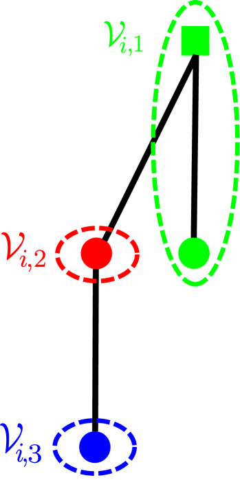
(a)

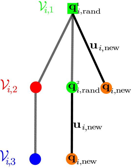
(b)

Figure 1: Fig. 1(a) shows an example of the sets $\mathcal{V}_{i,k}$. The root of the tree is depicted by a square. There are three ($K_{i,n}=3)$ groups $\mathcal{V}_{i,k}$ and the members of each group have the same color. Group $\mathcal{V}_{i,1}$ consists of nodes $\mathbf{q}_{i}^{1}$ and $\mathbf{q}_{i}^{2}$ for which $\mathbf{p}_{i}^{1}=\mathbf{p}_{i}^{2}$. Figure 1(b) illustrates the incremental construction of the tree.

III-A1 Sampling Strategy

The sampling procedure begins by first dividing the set of nodes $\mathcal{V}_{i}$ into a finite number of sets $\mathcal{V}_{i,k}\subseteq\mathcal{V}_{i}$. If $K_{i,n}$ is the number of created sets during iteration $n$ then $\mathcal{V}_{i}=\mathop{\cup}_{k=1}^{K_{i,n}}\mathcal{V}_{i,k}$. The set $\mathcal{V}_{i,k}$ collects nodes $\mathbf{q}_{i}=[\mathbf{p}_{i},\Sigma_{i},\mathcal{S}_{i}]\in\mathcal{V}_{i}$ that share the same robot state $\mathbf{p_{i}}$; see Fig. 1(a). At iteration $n=1$ it holds that $K_{i,1}=1$ and $\mathcal{V}_{i}=\mathcal{V}_{i,1}$ [line 1, Alg. 1]. Once the sets $\mathcal{V}_{i,k}$ are created, the nodes $\mathbf{q}_{i,\text{rand}}\in\mathcal{V}_{i,k_{i,\text{rand}}}$ will be expanded where index $k_{i,\text{rand}}$ is sampled from a given distribution $f_{\mathcal{V}_{i}}(k_{i}|\mathcal{V}_{i})\colon\{1,\dots,K_{i,n}\}\rightarrow[0,1]$ and points to the set $\mathcal{V}_{i,k_{i,\text{rand}}}$[line 1, Alg. 1].

Given nodes $\mathbf{q}_{i,\text{rand}}$ to be expanded with corresponding robot state $\mathbf{p}_{i,\text{rand}}$, a control input $\mathbf{u}_{i,\text{new}}$ is sampled from a distribution $f_{\mathcal{U}_{i}}(\mathbf{u}_{i})\colon\mathcal{U}_{i}\rightarrow[0,1]$. The new robot state $\mathbf{p}_{i,\text{new}}$ is created by applying the selected control input $\mathbf{u}_{i,\text{new}}$ to $\mathbf{p}_{i,\text{rand}}$ according to (1) [line 1, Alg. 1].

Remark 1 (Diversity of trees)

The selection of which group $\mathcal{V}_{i,k}$ is expanded is independent between different robots. Due to the randomness imposed by the aforementioned sampling procedures, the constructed trees $\mathcal{G}_{i}$ at iteration $n$ may have different structures among the robots.

III-A2 Extending the tree

Once $\mathbf{p}_{i,\text{new}}$ is constructed, we check whether it belongs to the obstacle-free area $\Omega_{\text{free}}$ or not. In the latter case, the sample is rejected and the sampling procedure is repeated [line 1, Alg. 1]. Otherwise, the state $\mathbf{q}_{i,\text{new}}$ is constructed; see Fig. 1(b). Specifically, given the parent node $\mathbf{q}_{i,\text{rand}}=[\mathbf{p}_{i,\text{rand}},\Sigma_{i,\text{rand}},\mathcal{S}_{i,\text{rand}}]$ and $\mathbf{p}_{i,\text{new}}$, the construction of $\mathbf{q}_{i,\text{new}}$ requires the computation of $\Sigma_{i,\text{new}}$ and $\mathcal{S}_{i,\text{new}}$. To what follows we assume that $\mathbf{q}_{i,\text{rand}}$ and $\mathbf{q}_{i,\text{new}}$ lie at depth $t$ and $t+1$ respectively. The update rule in (4) requires covariance matrix $\Sigma_{i}(t)$ obtained from node $\mathbf{q}_{i}(t)$ and $\Sigma_{j}(t)$ from neighbors $j\in\mathcal{N}_{i}$. From Remark 1, at depth $t$ there may exist more than one nodes $\mathbf{q}_{j}(t)\in\mathcal{V}_{j}$ to provide $\Sigma_{j}(t)$ or no nodes. Moreover, the covariance matrix $\Sigma_{i}(t)$ of node $\mathbf{q}_{i}(t)$ was once constructed using information received by the set of nodes $\mathcal{S}_{i}(t)=\{\mathbf{q}_{j}(t-1)\mid\Sigma_{j}(t-1)\textit{\text{ participated in computation of }}\Sigma_{i}(t)\textit{\text{ in \eqref{eq:distributed_kalman_filter}}},\forall\ j\in\mathcal{N}_{i}\}$, with $|\mathcal{S}_{i}(t)|=|\mathcal{N}_{i}|$ and $[\mathcal{S}_{i}(t)]_{j}=\mathbf{q}_{j}(t-1)$. To maintain consistency with the update rule in (4) only children of the set of nodes $\mathcal{S}_{i}(t)$ are allowed to distribute their corresponding covariance matrices. For every robot $j\in\mathcal{N}_{i}$ the set of admissible nodes to share $\Sigma_{j}(t)$ with robot $i$ is $\mathcal{Q}_{ij}(t)=\{\mathbf{q}_{j}(t)\mid\mathbf{q}_{j}(t)\textit{ is child of node }[\mathcal{S}_{i}(t)]_{j}\}$. Given the set $\mathcal{Q}_{ij}(t)$ node $\tilde{\mathbf{q}}_{j}(t)$ is sampled from a given discrete distribution $f_{\mathcal{Q}_{i}}(\mathbf{q}_{j})\colon\mathcal{Q}_{ij}(t)\rightarrow[0,1]$ and the set $\mathcal{S}_{i}(t+1)$ is created by collecting the sampled nodes from all $j\in\mathcal{N}_{i}$ [lines 1-1, Alg. 1]; see also Fig. 2. The covariance matrix $\Sigma_{i}(t+1)$ is then computed by applying the update rule in (4) and node $\mathbf{q}_{i,\text{new}}(t+1)$ is completed [lines 1-1, Alg. 1].

Next, the set of nodes and edges are updated and the cost of node $\mathbf{q}_{i,\text{new}}$ is computed as $J_{\mathcal{G}_{i}}(\mathbf{q}_{i,\text{new}}(t+1))=J_{\mathcal{G}_{i}}(\mathbf{q}_{i,\text{rand}}(t))+\det\Sigma_{i,\text{new}}(t+1)$ [lines 1-1, Alg. 1]. Finally, the sets $\mathcal{V}_{i,k}$ are updated, so that if there already exists a subset $\mathcal{V}_{i,k}$ with the same configuration as the state $\mathbf{p}_{i,\text{new}}$, then $\mathcal{V}_{i,k}=\mathcal{V}_{i,k}\cup\{\mathbf{q}_{i,\text{new}}(t+1)\}$. Otherwise, a new subset $\mathcal{V}_{i,k}=\{\mathbf{q}_{i,\text{new}}\}$ is created and the number of subsets increases by one, i.e. $K_{i,n}=K_{i,n}+1$ [lines 1-1, Alg. 1].

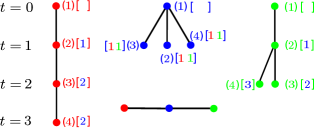
Figure 2: This Figure illustrates the computation of $\Sigma_{i,\text{new}}$ and $\mathcal{S}_{i,\text{new}}$ for a group of three robots, $i\in$ {red, blue, green}. The communication graph is depicted at the bottom. The growth of the trees for four iterations is presented where node $(k)$ is added to the trees. In square brackets, sets $\mathcal{S}_{i}$ are described. Red node $(4)$ awaits information from the blue robot, while the parent red node $(3)$ transmits its own $\mathcal{S}_{\text{red}}$, i.e. informs that it once communicated with the blue node $(2)$. Blue node $(2)$ is a leaf therefore $\mathcal{Q}_{\text{red}}=\{2\}$ and so $\mathcal{S}_{\text{red},\text{new}}=[2]$. Similarly for green node $(4)$, $\mathcal{Q}_{\text{green}}=\{2,3,4\}$ and blue node $(3)$ is sampled from $f_{\mathcal{Q}}$ to constitute $\mathcal{S}_{\text{green},\text{new}}$.

Remark 2 (Communication)

The update of $\Sigma_{i,\text{new}}$ in Section III-A2 is the only procedure for which robots need to communicate with each other to build their trees. The information robot $i$ sends to neighbors $\mathcal{N}_{i}$ is the set $\mathcal{S}_{i,\text{rand}}$. In exchange it receives covariance matrices $\Sigma_{j}$.

Remark 3 (Set of candidate nodes)

In the case where the set of candidate nodes $\mathcal{Q}_{ij}(t)$ is empty, covariance matrix of node $[\mathcal{S}_{i}(t)]_{j}$ will be transmitted.

IV Complexity, Completeness and Optimality

In this section, we show that Algorithm 1 reduces the computational complexity per iteration of its centralized counterpart [28]. We further show that it is probabilistically complete and asymptotically optimal under the following assumptions regarding the mass functions $f_{\mathcal{V}_{i}},f_{\mathcal{U}_{i}},f_{\mathcal{Q}_{i}}$. The proofs of the following results can be found in Section VIII.

Assumption 2 (Probability mass function $f_{\mathcal{V}_{i}}$)

(i) Pr-
obability mass function $f_{\mathcal{V}_{i}}(k_{i}|\mathcal{V}_{i})\colon\{1,\dots,K_{i,n}\}\rightarrow[0,1]$ satisfies $f_{\mathcal{V}_{i}}(k_{i}|\mathcal{V}_{i})\geq\epsilon,\forall k_{i}\in\{1,\dots,K_{i,n}\},\forall n\geq 0$ for some $\epsilon>0$ that remains constant across all iterations (ii) $k_{i,\text{rand}}$ are drawn independently across iterations.

Assumption 3 (Probability mass function $f_{\mathcal{U}_{i}}$)

(i) Pr-
obability mass function $f_{\mathcal{U}_{i}}$ satisfies $f_{\mathcal{U}_{i}}(\mathbf{u}_{i})\geq\zeta,\forall\mathbf{u}_{i}\in\mathcal{U}_{i},\forall n\geq 0$, for some $\zeta>0$ that remains constant across all iterations (ii) Samples $\mathbf{u}_{i}$ are drawn independently across iterations.

Assumption 4 (Probability mass function $f_{\mathcal{Q}_{i}}$)

(i) Pr-
obability mass function $f_{\mathcal{Q}_{i}}$ satisfies $f_{\mathcal{Q}_{i}}(\mathbf{q}_{j})\geq\xi,\forall\mathbf{q}_{j}\in\mathcal{Q}_{ij},\forall n\geq 0$, where $\xi>0$ (ii) Samples $\mathbf{q}_{j}$ are drawn independently across iterations.

Remark 4 (Mass functions)

Assumptions 2-4 are defined in such a way to ensure that the sets (i) $\{1,\dots,K_{i,n}\}$, (ii) $\mathcal{U}_{i}$ and (iii) $\mathcal{Q}_{ij}$ have non-zero measure. They are important to ensure the exploration of the entire physical and reachable information space and the fusion of potential beliefs for the DKF. All of them are very flexible, since they allow $f_{\mathcal{V}_{i}},f_{\mathcal{U}_{i}}$ and $f_{\mathcal{Q}_{i}}$ to change with iterations of Algorithm 1, as the trees grow and to be different among the robots. Any mass functions could be used as long as they satisfy the aforementioned assumptions. A typical example is the discrete uniform distribution. In Section V non-uniform distributions are suggested for a target-tracking scenario.

Theorem 1 (Probabilistic Completeness)

If there exists a solution to Problem 6, then Algorithm 1 is probabilistically complete, i.e., feasible paths $\bm{q}_{i,0:F}=\bm{q}_{i}(0),\dots,\bm{q}_{i}(F)$, $\bm{q}_{i}(f)\in\mathcal{V}_{i}$, for all $f\in\{0,\dots,F\}$ and $i\in\{1,\dots,N\}$, will be found with probability $1$, as $n\to\infty$.

Theorem 2 (Asymptotic Optimality)

Assume that there exists an optimal solution to Problem 6. Then, Algorithm 1 is asymptotically optimal, i.e., the optimal paths $\bm{q}_{i,0:F}^{*}=\bm{q}_{i}(0),\bm{q}_{i}(1),\bm{q}_{i}(2),\dots,\bm{q}_{i}(F)$ for all $i=\{1,\dots,N\}$, will be found with probability $1$, as $n\to\infty$.

Theorem 3 (Complexity Per Iteration)

Let $d_{\max}$ denote the maximum degree of the vertices of the communication graph $G$, $N$ be the number of robots and $k$ be the number of nodes $\mathbf{q}_{\text{rand}}$ to be expanded in one iteration. Then the computational complexity per iteration of Algorithm 1 and the centralized approach [28] is $\mathcal{O}(kd_{\max})$ and $\mathcal{O}(kN)$ respectively, under a worst-case scenario complexity analysis.

V Biased Sampling - Target Tracking

In large-scale estimation problems where a large number of robots are equipped to estimate high-dimensional hidden states, mass functions $f_{\mathcal{V}_{i}},f_{\mathcal{U}_{i}}$ and $f_{\mathcal{S}_{i}}$ introduced in Section III could be designed such that the trees tend to explore regions that are expected to be informative. In this section, we consider an application to target localization for Algorithm 1. The hidden state $\mathbf{x}(t)$ now collects the positions of all targets at time $t$, i.e $\mathbf{x}(t)=[\mathbf{x}_{1}(t)^{T},\dots,\mathbf{x}_{M}(t)^{T}]^{T}$, where $\mathbf{x}_{l}(t)$ is the position of target $l$ at time $t$ and $M$ is the number of targets. In this application, we require the constraint (6f) to hold for all targets $\mathbf{x}_{l}(F+1)$ for some $\delta_{i}^{l}$, i.e $\det\Sigma_{i}^{l}\leq\delta_{i}^{l}$ where $\Sigma_{i}^{l}$ is the corresponding covariance matrix of target $l$. In what follows, we design mass functions that allow us to address large-scale estimation tasks that involve large teams of robots and targets.

V-A Mass function $f_{\mathcal{V}_{i}}$

Let $L_{i,\max}^{n}$ denote the depth of tree $\mathcal{G}_{i}$ at iteration $n$ and $\mathcal{K}_{i,\max}^{n}$ be the set that collects indices $k$ that point to subsets $\mathcal{V}_{i,k}$ for which there exists at least a node $\mathbf{q}_{i}\in\mathcal{V}_{i,k}$ that lays at depth $L_{i,\max}^{n}.$ Given the set $\mathcal{K}_{i,\max}^{n}$ the mass function $f_{\mathcal{V}_{i}}$ is designed as follows

$$f_{\mathcal{V}_{i}}(k|\mathcal{V}_{i})=\left\{\begin{array}[]{ll}p_{\mathcal{V}_{i}}\frac{1}{|\mathcal{K}_{i,\text{max}}^{n}|},~{}~{}~{}~{}~{}~{}~{}~{}~{}~{}~{}~{}\mbox{if}~{}k\in\mathcal{K}_{i,\text{max}}^{n}\\ (1-p_{\mathcal{V}_{i}})\frac{1}{|\mathcal{V}_{i}\setminus\mathcal{K}_{i,\text{max}}^{n}|},~{}\mbox{otherwise},\end{array}\right.$$ (8)

where $p_{\mathcal{V}_{i}}\in(0.5,1)$ is the probability of selecting any group $\mathcal{V}_{i,k}$ indexed by $k\in\mathcal{K}_{i,\max}^{n}$.

V-B Mass function $f_{\mathcal{U}_{i}}$

The mass function $f_{\mathcal{U}_{i}}$ is designed such that control inputs that drive robot $i$ with position $\mathbf{p}_{i}(t)$ closer to target $j$ of predicted position $\hat{\mathbf{x}}_{j}(t+1)$ at time $t+1$ are selected more often. If $\bm{u}_{i}^{*}$ is the control input that minimizes the geodesic distance between $\bm{p}_{i}(t+1)$ and $\hat{\bm{x}}_{j}(t+1)$, i.e $\bm{u}_{i}^{*}=\arg\min_{\bm{u}\in\mathcal{U}_{i}}\left[d_{ij}=\parallel\bm{p}_{i}(t+1)-\hat{\bm{x}}_{j}(t+1)\parallel_{g}\right]$ the mass function $f_{\mathcal{U}_{i}}$ is constructed as follows

$$f_{\mathcal{U}_{i}}(\bm{u}_{i})=\left\{\begin{array}[]{ll}p_{\mathcal{U}_{i}},~{}~{}~{}~{}~{}~{}~{}~{}~{}~{}~{}~{}\mbox{if}~{}(\bm{u}_{i}=\bm{u}_{i}^{*})\wedge(d_{ij}>R_{i})\\ (1-p_{\mathcal{U}_{i}})\frac{1}{|\mathcal{U}_{i}|},~{}\mbox{otherwise},\end{array}\right.$$ (9)

where (i) $p_{\mathcal{U}_{i}}\in(0.5,1)$ is the probability that input $\mathbf{u}_{i}$ is selected (ii) $\mathbf{p}_{i}(t+1)$ is computed as per (1) (iii) $\hat{\mathbf{x}}_{j}(t+1)$ is the predicted position of target $j$ from the Kalman filter prediction step and (iv) $R_{i}$ denotes the sensing range. Once the predicted position $\hat{\mathbf{x}}_{j}(t+1)$ is within the robot’s sensing range, controllers are selected randomly.

V-C Mass function $f_{\mathcal{S}_{i}}$

The mass function $f_{\mathcal{S}_{i}}$ is designed such that when more than one candidate nodes $\mathbf{q}_{j}\in\mathcal{Q}_{ij}$ are available, node $\mathbf{q}_{j}^{*}$ with the smallest uncertainty, i.e $|\Sigma_{j}^{*}|=\arg\min_{\mathbf{q}_{j}\in\mathcal{Q}_{ij}}|\Sigma_{j}|$ is selected with higher probability. Given the set $\mathcal{Q}_{ij}$ the mass function $f_{\mathcal{S}_{i}}$ is the following

$$f_{\mathcal{S}_{i}}(\bm{q}_{j})=\left\{\begin{array}[]{ll}p_{\mathcal{S}_{i}},~{}~{}~{}~{}~{}~{}~{}~{}~{}~{}~{}~{}\mbox{if}~{}\bm{q}_{j}=\bm{q}_{j}^{*}\\ (1-p_{\mathcal{S}_{i}})\frac{1}{|\mathcal{Q}_{ij}|},~{}\mbox{otherwise},\end{array}\right.$$ (10)

where $p_{\mathcal{S}_{i}}\in(0.5,1)$ is the probability that node $\mathbf{q}_{j}$ is selected to provide covariance matrix $\Sigma_{j}(t)$.

V-D On-the-fly Target Assignment

In Algorithm 2 we propose a target assignment process executed once the state $\mathbf{q}_{i,\text{new}}$ is created. Initially robot $i$ inherits the assigned target $l_{i,\text{rand}}$ of the parent node $\mathbf{q}_{i,\text{rand}}$. Initially the sets $\mathcal{T}_{i,\text{sorted}},\mathcal{T}_{i,\text{satisfied}},\mathcal{T}_{i,\text{unsatisfied}}$ and $\mathcal{T}_{i,\text{occupied}}$ are created [Alg. 2, lines 2-2]. In particular, the set $\mathcal{T}_{i,\text{sorted}}$ is the sorted set of indices $l\in\{1,\dots,M\}$ of increasing order according to the geodesic distance $\parallel\mathbf{p}_{i,\text{new}}-\hat{\mathbf{x}}_{l}\parallel_{g}$. Moreover, the set $\mathcal{T}_{i,\text{satisfied}}$ collects the indices of the satisfied targets, i.e $\mathcal{T}_{i,\text{satisfied}}=\{l\mid\det\Sigma_{i,\text{new}}^{l}\leq\delta_{i}^{l},\ l\in\{1,\dots,M\}\}$ [line 2, Alg. 2]. Given the aforementioned sets, we can compute the sorted set of the unsatisfied targets $\mathcal{T}_{i,\text{unsatisfied}}$ [line 2, Alg. 2]. The set $\mathcal{T}_{i,\text{occupied}}$ collects the indices $l_{j}$ that point to targets already assigned to neighbors $\mathcal{N}_{i}$, i.e $\mathcal{T}_{i,\text{occupied}}=\{l_{j}\mid\text{{assigned target of }}\mathbf{q}_{j}\in\mathcal{Q}_{ij},j\in\mathcal{N}_{i}\}$ [line 2, Alg. 2]. Once the sets are computed the robot sequentially seeks for the new target $l_{i,new}$ that is not already assigned to any of the neighbors and has not satisfied the uncertainty threshold [Alg. 2, lines 2-2].

Input: (i) $\delta_{k},\forall k\in\{1,\dots M\}$, (ii) $\mathbf{q}_{i,\text{new}}$, (iii) current target $l_{\text{i,rand}}$

Output: assigned target $l_{i,\text{new}}$

1 Compute sets $\mathcal{T}_{i,\text{sorted}}$ and $\mathcal{T}_{i,\text{satisfied}}$;

2 Compute set $\mathcal{T}_{i,\text{unsatisfied}}=\mathcal{T}_{i,\text{sorted}}\backslash\mathcal{T}_{i,\text{satisfied}}$;

3 Compute set $\mathcal{T}_{i,\text{occupied}}$;

4 $l_{i,\text{new}}=[\ ]$;

5 for $l\in\mathcal{T}_{i,\text{unsatisfied}}$ do

6       if $l\notin\mathcal{T}_{i,\text{occupied}}$ then

7             $l_{i,\text{new}}=l$;

8             break;

9            

10if $l_{i,\text{new}}$ is empty then

11       $l_{i,\text{new}}=l_{i,\text{rand}}$;

12      

Algorithm 2 On-the-fly Target Assignment

VI Numerical Experiments

In this section, we present numerical experiments that illustrate the performance of Algorithm 1 for the target localization and tracking problem, described in Section V. We are interested in examining the scalability of Algorithm 1 and compare performances for different communication networks. All case studies have been implemented using Python 3.6 on a computer with Intel Core i10 1.3GHz and 16Gb RAM.

In this section, each robot uses differential drive dynamics with $\mathbf{p}_{i}(t)$ describing the position and orientation of robot $i$ at time $t$. The control commands use motion primitives $\{\nu_{i},\omega_{i}\},\ \nu_{i}\in\{0,0.2,1\}\text{m/s},\ \omega_{i}\in\{0,\pm 5,\pm 10,\pm 20,\pm 30,\\ \pm 45,\pm 60\}^{\circ}\text{/s}.$ Furthermore, we assume that the robots are equipped with omnidirectional, range-only, line-of-sight sensors with limited range of 1m. The measurement received by robot $i$ regarding target $k$ is given by $y_{i,k}=l_{i,k}(t)+v_{i}(t)$ if $(l_{i,k}(t)\leq 1)\wedge(k\in\texttt{FOV}_{i})$ where $l_{i,k}(t)$ is the distance between robot $i$ and target $k$, $\texttt{FOV}_{i}$ denotes the field-of-view of robot $i$ and $v_{i}(t)\sim\mathcal{N}(0,\sigma^{2}(\mathbf{p}_{i}(t),\mathbf{x}_{k}(t))$ is the measurement noise with $\sigma=0.25l_{i,k}(t)$ if $l_{i,k}(t)\leq 1$; otherwise $\sigma$ is infinite. For separation principle to hold and offline control policies to be optimal we linearize the observation model about the predicted target position. In all case studies the targets are modeled as linear systems and the threshold parameter is selected to be $\delta_{i}^{k}=1.8\times 10^{-5}$ for all targets. The robots reside in the $10m\times 10m$ environment shown in Fig. 4. The DKF parameters are chosen as $k_{ii}=0.75$ and $k_{ij}=0.25/|\mathcal{N}_{i}|$ if $\det\Sigma_{i}^{l}\leq\det\Sigma_{j}^{l}$ for a target $l$; otherwise the values interchange.

VI-A Scalability Performance

In this Section we examine the scalability of the proposed distributed scheme with respect to the number of robots $N$ and targets $M$ for different communication networks. In Table I we provide averaged results from ten Monte-Carlo trials for random and fully connected communication networks and the centralized approach in [28]. Especially for the random communication networks we state the average degree (A.D) of the vertices pointing to the robots. The results come from a sequential implementation of Algorithm 1 and the time required by the ”slowest” robot to build its tree is reported in Table I for the distributed scheme.

TABLE I: Scalability Analysis

	Connected		All-to-All	Centralized
N/M	A.D	Runtime / F	Runtime / F	Runtime / F
10/10	5.60	2.09 secs / 28	1.45 secs / 15	7.670 secs / 11
10/20	5.00	3.63 secs / 33	2.93 secs / 26	15.03 secs / 18
10/35	5.40	5.69 secs / 40	3.37 secs / 25	25.37 secs / 19
15/20	8.10	2.72 secs / 26	2.60 secs / 26	14.30 secs / 13
15/35	8.50	4.41 secs / 34	3.77 secs / 26	25.24 secs / 15
20/20	11.1	2.93 secs / 28	2.11 secs / 17	23.14 secs / 14
20/25	10.5	4.00 secs / 33	2.51 secs / 19	21.27 secs / 12
20/35	10.7	4.64 secs / 32	3.51 secs / 24	26.02 secs / 11
30/50	17.0	5.32 secs / 26	4.29 secs / 19	46.02 secs / 10

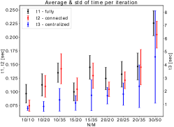
Figure 3: This Figure illustrates the average time needed for a completion of one iteration across the entire planning horizon $F$ for $N$ robots, $M$ targets for three cases (i) random connected network (red), (ii) fully connected network (black) and (iii) centralized method (blue).

We can notice that feasible paths are computed very fast for all connectivity cases regardless of the number of robots and targets. The planning horizon $F$ of the random connected networks is always larger since any transmitted information needs more timesteps until diffused. The centralized approach returns the smallest $F$, as in contrast to DKF the update rule of Kalman Filter fuses measurement models of all robots and therefore the desired uncertainty threshold is reached faster. In Fig. 3 the average time of completion of one iteration is presented for all scenarios of Table I. We can see that the distributed approach improves the computational complexity per iteration by at least a factor of 10.

VI-B Different communication networks

In this section we examine the performance of Algorithm 1 for different communication graph densities. Specifically, in Fig. 4, the trajectories for three different communication scenarios are presented for $N=6$ robots and $M=10$ targets (i) fully connected graph (ii) connected graph with three edges average degree and (iii) no communication. In the current example, the planning terminates once a robot realizes that the targets have been identified either by itself and/or by any of the neighboring robots.

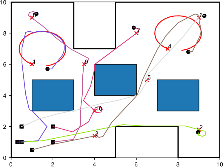
(a)

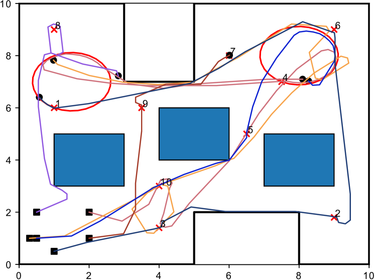
(b)

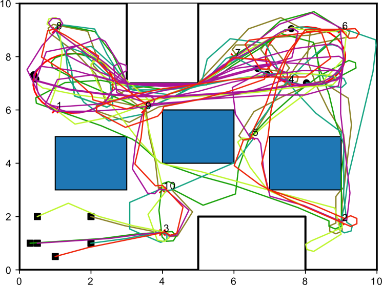
(c)

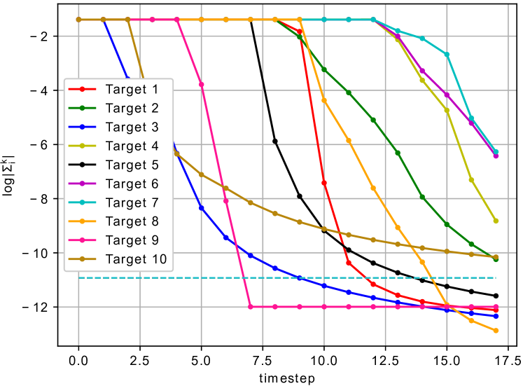
(d)

Figure 4: Trajectories of $N=6$ robots and $M=10$ targets for three communication networks (a) fully connected, (b) connected and (c) no communication. The initial positions of the targets are depicted as red crosses and the trajectory of moving targets can be seen in solid red color. The initial and final position of the robots are depicted by black squares and circles respectively. In Fig. 4(d) the uncertainties $\det\Sigma_{i}^{k}$ are presented for the ”purple” robot of Fig. 4(a). The dashed line depicts the threshold $\delta_{i}^{k}$.

The density of the communication network affects the returned paths and the planning horizon $F$. Specifically, in the case of a fully connected network as in Fig. 4(a) the speed of fusing beliefs is high and thus robots reduce their uncertainty even for targets that have not been visited by themselves. The same idea extends in the case of a random connected network as in Fig. 4(b) with the only difference being that the fusion of beliefs has a smaller rate and therefore robots may revisit targets that have already been satisfied. In fact the less dense a graph is the more the planning horizon $F$ increases. In the case of no communication in Fig. 4(c) each robot plans completely on its own and therefore every target is visited. Kalman Filter updates may lead to an increase of the uncertainty over a dynamic target even if in the past it was well estimated. The robots then as in Fig. 4(c) oscillate between the two moving targets leading to a further increase of their planning horizon. The returned planning horizons of the aforementioned cases are $F=[24,29,120]$, where for the disconnected network the maximum planning horizon out of the individual planning horizons of each robot is stated.

In Fig. 4(d) the evolution of the uncertainties $\det\Sigma_{i}^{k}$ over time is depicted for the ”purple” robot of the fully connected case of Fig. 4(a). Thanks to the connectivity capabilities, we can see that the current robot has not reduced the uncertainty for the entire group of targets since it realizes that there exist other robots that took the responsibility of identifying the remaining targets.

VII Conclusions

A new distributed sampling-based algorithm for active information gathering is introduced in this paper followed by formal guarantees. The proposed scheme is tested via extensive simulations showing that feasible paths are quickly computed for large-scale problems, improving significantly also the computational time of existing scalable centralized method. In the future, time-varying communication graphs will be incorporated in the proposed framework.

VIII Appendix: Proof of Separation Principle, Completeness & Optimality

To prove Theorems 1, 2 we need to prove the following results.

Lemma 1

(Sampling $\mathcal{V}^{n}_{i,k_{\text{rand}}}$) Consider any subset $\mathcal{V}_{i,k}^{n}$, any fixed iteration index $n$ and any fixed $k\in\{1,\dots,K_{i,n}\}$. Then, there exists an infinite number of subsequent iterations $n+w$, where $w\in\mathcal{W}$ and $\mathcal{W}\subseteq\mathbb{N}$ is a subsequence of $\mathbb{N}$, at which the subset $\mathcal{V}_{i,k}^{n}$ is selected to be the set $\mathcal{V}_{i,k_{\text{rand}}}^{n+w}$.

Lemma 2 (Sampling $\bm{u}_{i,\text{new}}$)

Consider any subset $\mathcal{V}_{i,k_{\text{rand}}}^{n}$ selected by $f_{\mathcal{V}_{i}}$ and any fixed iteration index $n$. Then, for any given control input $\bm{u}\in\mathcal{U}_{i}$, there exists an infinite number of subsequent iterations $n+w$, where $w\in\mathcal{W}^{\prime}$ and $\mathcal{W}^{\prime}\subseteq\mathcal{W}$ is a subsequence of the sequence of $\mathcal{W}$ defined in Lemma 1, at which the control input $\bm{u}\in\mathcal{U}_{i}$ is selected to be $\bm{u}_{i,\text{new}}^{n+w}$.

Proof:

The proofs of Lemmas 1, 2 resemble the proof of [28, Appendix A] and are omitted. ∎

Lemma 3

(Sampling $\mathbf{q}_{j}$) Consider any subset $\mathcal{V}_{i,k_{\text{rand}}}^{n}$, any control input $\bm{u}_{i,\text{new}}$ and any fixed iteration $n$. Then for any $\mathbf{q}_{j}\in\mathcal{Q}_{ij}^{n}$ there exists an infinite number of subsequent iterations $n+w$, where $w\in\mathcal{W}^{\prime\prime}$ and $\mathcal{W}^{\prime\prime}\subseteq\mathcal{W}^{\prime}$ is a subsequence of the sequence $\mathcal{W}^{\prime}$ defined in Lemma 2, at which node $\mathbf{q}_{j}$ is selected to be added in the set $\mathcal{S}_{i,new}$.

Proof:

Define the infinite sequence of events $A^{\text{new}}=\{A^{\text{new},n+w}(\bm{q}_{j})\}_{w=0}^{\infty}$, for $\bm{q}_{j}\in\mathcal{Q}_{ij}^{n}$, where $A^{\text{new},n+w}(\bm{q}_{j})=\{\bm{q}_{j}^{n+w}=\bm{q}_{j}\}$, for $w\in\mathbb{N}$, denotes the event that at iteration $n+w$ of Algorithm 1 node $\bm{q}_{j}\in\mathcal{Q}_{ij}^{n}$ is selected by the sampling function to be the node $\bm{q}_{j}^{n+w}$, given the subset $\mathcal{V}_{i,k_{\text{rand}}}^{n}\in\mathcal{V}_{k_{\text{rand}}}^{n+w}$ and control input $\mathbf{u}_{i,\text{new}}$. Moreover, let $\mathbb{P}(A^{\text{new},n+w}(\bm{q}_{j}))$ denote the probability of this event, i.e., $\mathbb{P}(A^{\text{new},n+w}(\bm{q}_{j}))=f_{\mathcal{Q}_{i}}^{n+w}(\bm{q}_{j}|\mathcal{Q}_{ij}^{n+w})$. Now, consider those iterations $n+w$ with $w\in\mathcal{W^{\prime}}$ such that $k_{\text{rand}}^{n+w}=k_{\text{rand}}^{n}$ and $\mathbf{u}_{i,\text{new}}^{n+w}=\mathbf{u}_{i,\text{new}}^{n}$ by Lemma 2. We will show that the series $\sum_{w\in\mathcal{W^{\prime}}}\mathbb{P}(A^{\text{new},n+w}(\bm{q}_{j}))$ diverges and then we will use Borel-Cantelli lemma to show that any given $\bm{q}_{j}\in\mathcal{U}$ will be selected infinitely often to be $\bm{q}_{j}^{n+w}$. By Assumption 4(i) we have that $\mathbb{P}(A^{\text{new},n+w}(\bm{q}_{j}))=f_{\mathcal{Q}_{i}}^{n+w}(\bm{q}_{j}|\mathcal{Q}_{ij}^{n+w})$ is bounded below by a strictly positive constant $\xi>0$ for all $w\in\mathcal{W}^{\prime}$. Therefore, we have that $\sum_{w\in\mathcal{W}^{\prime}}\mathbb{P}(A^{\text{new},n+w}(\bm{q}_{j}))$ diverges, since it is an infinite sum of a strictly positive constant term. Using this result along with the fact that the events $A^{\text{new},n+w}(\bm{q}_{j})$ are independent, by Assumption 4 (ii), we get that $\mathbb{P}(\limsup_{w\to\infty}A^{\text{new},n+w}(\bm{q}_{j}))=1,$ due to the Borel-Cantelli lemma. In words, this means that the events $A^{\text{new},n+w}(\bm{q}_{j})$ for $w\in\mathcal{W}^{\prime}$ occur infinitely often. Thus, given any subset $\mathcal{V}_{i,k_{\text{rand}}}^{n}$, any control input $\bm{u}_{i,\text{new}}^{n}$ for all $q_{j}\in\mathcal{Q}_{ij}^{n}$ and for all $n\in\mathbb{N}_{+}$, there exists an infinite subsequence $\mathcal{W}^{\prime\prime}\subseteq\mathcal{W}^{\prime}$ so that for all $w\in\mathcal{W}^{\prime\prime}$ it holds $\bm{q}_{j}^{n+w}=\bm{q}_{j}$, completing the proof. ∎

Before stating the next result, we first define the reachable state-space of a state $\bm{q}_{i}(t)=[\bm{p}_{i}(t),\Sigma_{i}(t),\mathcal{S}_{i}(t)]\in\mathcal{V}_{i,k}^{n}$, denoted by $\mathcal{R}(\bm{q}_{i}(t))$ that collects all states $\bm{q}_{i}(t+1)=[\bm{p}_{i}(t+1),\Sigma_{i}(t+1),\mathcal{S}_{i}(t+1)]$ that can be reached within one time step from $\bm{q}_{i}(t)$.

Corollary 1 (Reachable set $\mathcal{R}(\bm{q}_{i}(t))$)

Given any state $\bm{q}_{i}(t)=[\bm{p}_{i}(t),\Sigma_{i}(t),\mathcal{S}_{i}(t)]\in\mathcal{V}_{i,k}^{n}$, for any $k\in\{1,\dots,K_{i,n}\}$, Algorithm 1 will add to $\mathcal{V}_{i}^{n}$ all states that belong to the reachable set $\mathcal{R}(\bm{q}_{i}(t))$ will be added to $\mathcal{V}_{i}^{n+w}$, with probability 1, as $w\to\infty$, i.e., $\lim_{w\rightarrow\infty}\mathbb{P}\left(\{\mathcal{R}(\bm{q}_{i}(t))\subseteq\mathcal{V}_{i}^{n+w}\}\right)=1.$ Also, edges from $\bm{q}_{i}(t)$ to all reachable states $\bm{q}_{i}^{\prime}(t+1)\in\mathcal{R}(\bm{q}_{i}(t))$ will be added to $\mathcal{E}_{i}^{n+w}$, with probability 1, as $w\to\infty$, i.e., $\lim_{w\rightarrow\infty}\mathbb{P}\left(\{\cup_{\bm{q}_{i}^{\prime}\in\mathcal{R}(\bm{q}_{i})}(\bm{q}_{i},\bm{q}_{i}^{\prime})\subseteq\mathcal{E}_{i}^{n+w}\}\right)=1.$

Proof:

The proof straightforwardly follows from Lemmas 1-3 and is omitted. ∎

Proof of Theorem 1: By construction of the path $\bm{q}_{i,0:F}$, it holds that $\bm{q}_{i}(f)\in\mathcal{R}(\bm{q}_{i}(f-1))$, for all $f\in\{1,\dots,F\}$. Since $\bm{q}_{i}(0)\in\mathcal{V}_{i}^{1}$, it holds that all states $\bm{q}_{i}\in\mathcal{R}(\bm{q}_{i}(0))$, including the state $\bm{q}_{i}(1)$, will be added to $\mathcal{V}_{i}^{n}$ with probability $1$, as $n\to\infty$, due to Corollary 1. Once this happens, the edge $(\bm{q}_{i}(0),\bm{q}_{i}(1))$ will be added to set of edges $\mathcal{E}_{i}^{n}$ due to Corollary 1. Applying Corollary 1 inductively, we get that $\lim_{n\rightarrow\infty}\mathbb{P}\left(\{\bm{q}_{i}(f)\in\mathcal{V}_{i}^{n}\}\right)=1$ and $\lim_{n\rightarrow\infty}\mathbb{P}\left(\{(\bm{q}_{i}(f-1),\bm{q}_{i}(f))\in\mathcal{E}_{i}^{n}\}\right)=1$, for all $f\in\{1,\dots,F\}$ meaning that the path $\bm{q}_{i,0:F}$ will be added to the tree $\mathcal{G}_{i}^{n}$ with probability $1$ as $n\to\infty$ completing the proof.

Proof of Theorem 2: The proof of this result straightforwardly follows from Theorem 1. Specifically, recall from Theorem 1 that Algorithm 1 can find any feasible path and, therefore, the optimal path as well, with probability 1, as $n\to\infty$, completing the proof.

Proof of Theorem 3: For the proof, a fixed iteration is considered and the computational complexity is analyzed with parameters the number of robots $N$ and maximum degree of the vertices $d_{\max}$ of the communication graph $G$, where $d_{\max}\leq N-1$. Let’s assume that both methods need to expand $k$ nodes $\mathbf{q}_{\text{rand}}$ and robot $i$ is the one with the most neighbors, i.e $d_{\max}=|\mathcal{N}_{i}|$. In the centralized approach [28] each state $\mathbf{p}_{\text{rand}}$ describes $N$ concatenated states $\mathbf{p}_{i,\text{rand}}$. The computation then of $\mathbf{p}_{\text{new}}$ is of order $\mathcal{O}(kN)$, while for Algorithm 1 is $\mathcal{O}(k)$. The Kalman filter update rule in [28] is computed based on $N$ measurement models, while in Algorithm 1 each state $\mathbf{p}_{i,\text{new}}$ uses information from $|\mathcal{N}_{i}|$ neighbors. The respective Kalman Filter complexities then are $\mathcal{O}(N)$ and $\mathcal{O}(k|\mathcal{N}_{i}|)$. Note that sampling a single-query from a discrete distribution and checking membership of $\mathbf{q}_{\text{new}}$ in a subset $\mathcal{V}_{k}$ depends on parameters which are not part of our analysis and are not taken into account. Summing-up, the computational complexity per iteration of centralized approach [28] and Algorithm 1 are $\mathcal{O}(kN+N)=\mathcal{O}(kN)$ and $\mathcal{O}(k+kd_{\text{max}})=\mathcal{O}(kd_{\text{max}})$ respectively, completing the proof.

References

• [1] K.-C. Ma, L. Liu, and G. S. Sukhatme, “Informative planning and online learning with sparse gaussian processes,” in 2017 IEEE International Conference on Robotics and Automation (ICRA).   IEEE, 2017, pp. 4292–4298.
• [2] Q. Lu and Q.-L. Han, “Mobile robot networks for environmental monitoring: A cooperative receding horizon temporal logic control approach,” IEEE transactions on cybernetics, vol. 49, no. 2, pp. 698–711, 2018.
• [3] E. W. Frew and J. Elston, “Target assignment for integrated search and tracking by active robot networks,” in 2008 IEEE International Conference on Robotics and Automation.   IEEE, 2008, pp. 2354–2359.
• [4] M. Tzes, S. Papatheodorou, and A. Tzes, “Visual area coverage by heterogeneous aerial agents under imprecise localization,” IEEE control systems letters, vol. 2, no. 4, pp. 623–628, 2018.
• [5] T. Kusnur, D. M. Saxena, and M. Likhachev, “Search-based planning for active sensing in goal-directed coverage tasks,” arXiv preprint arXiv:2011.07383, 2020.
• [6] D. J. Bucci and P. K. Varshney, “Decentralized multi-target tracking in urban environments: Overview and challenges,” in 2019 22th International Conference on Information Fusion (FUSION).   IEEE, 2019, pp. 1–8.
• [7] G. Huang, K. Zhou, N. Trawny, and S. I. Roumeliotis, “A bank of maximum a posteriori (map) estimators for target tracking,” IEEE Transactions on Robotics, vol. 31, no. 1, pp. 85–103, 2015.
• [8] L. Carlone, J. Du, M. K. Ng, B. Bona, and M. Indri, “Active slam and exploration with particle filters using kullback-leibler divergence,” Journal of Intelligent & Robotic Systems, vol. 75, no. 2, pp. 291–311, 2014.
• [9] N. Atanasov, J. Le Ny, K. Daniilidis, and G. J. Pappas, “Decentralized active information acquisition: Theory and application to multi-robot slam,” in 2015 IEEE International Conference on Robotics and Automation (ICRA).   IEEE, 2015, pp. 4775–4782.
• [10] ——, “Information acquisition with sensing robots: Algorithms and error bounds,” in 2014 IEEE International Conference on Robotics and Automation (ICRA).   IEEE, 2014, pp. 6447–6454.
• [11] N. Atanasov, R. Tron, V. M. Preciado, and G. J. Pappas, “Joint estimation and localization in sensor networks,” in 53rd IEEE Conference on Decision and Control.   IEEE, 2014, pp. 6875–6882.
• [12] T. H. Chung, J. W. Burdick, and R. M. Murray, “A decentralized motion coordination strategy for dynamic target tracking,” in Proceedings 2006 IEEE International Conference on Robotics and Automation, 2006. ICRA 2006.   IEEE, 2006, pp. 2416–2422.
• [13] R. Olfati-Saber, “Distributed tracking for mobile sensor networks with information-driven mobility,” in 2007 American Control Conference.   IEEE, 2007, pp. 4606–4612.
• [14] G. M. Hoffmann and C. J. Tomlin, “Mobile sensor network control using mutual information methods and particle filters,” IEEE Transactions on Automatic Control, vol. 55, no. 1, pp. 32–47, 2009.
• [15] P. Dames, M. Schwager, V. Kumar, and D. Rus, “A decentralized control policy for adaptive information gathering in hazardous environments,” in 2012 IEEE 51st IEEE Conference on Decision and Control (CDC).   IEEE, 2012, pp. 2807–2813.
• [16] B. Charrow, V. Kumar, and N. Michael, “Approximate representations for multi-robot control policies that maximize mutual information,” Autonomous Robots, vol. 37, no. 4, pp. 383–400, 2014.
• [17] F. Meyer, H. Wymeersch, M. Fröhle, and F. Hlawatsch, “Distributed estimation with information-seeking control in agent networks,” IEEE Journal on Selected Areas in Communications, vol. 33, no. 11, pp. 2439–2456, 2015.
• [18] M. Corah and N. Michael, “Distributed submodular maximization on partition matroids for planning on large sensor networks,” in 2018 IEEE Conference on Decision and Control (CDC).   IEEE, 2018, pp. 6792–6799.
• [19] J. Le Ny and G. J. Pappas, “On trajectory optimization for active sensing in gaussian process models,” in Proceedings of the 48h IEEE Conference on Decision and Control (CDC) held jointly with 2009 28th Chinese Control Conference.   IEEE, 2009, pp. 6286–6292.
• [20] A. Singh, A. Krause, C. Guestrin, and W. J. Kaiser, “Efficient informative sensing using multiple robots,” Journal of Artificial Intelligence Research, vol. 34, pp. 707–755, 2009.
• [21] B. Schlotfeldt, D. Thakur, N. Atanasov, V. Kumar, and G. J. Pappas, “Anytime planning for decentralized multirobot active information gathering,” IEEE Robotics and Automation Letters, vol. 3, no. 2, pp. 1025–1032, 2018.
• [22] C. B. Browne, E. Powley, D. Whitehouse, S. M. Lucas, P. I. Cowling, P. Rohlfshagen, S. Tavener, D. Perez, S. Samothrakis, and S. Colton, “A survey of monte carlo tree search methods,” IEEE Transactions on Computational Intelligence and AI in games, vol. 4, no. 1, pp. 1–43, 2012.
• [23] G. Best, O. M. Cliff, T. Patten, R. R. Mettu, and R. Fitch, “Dec-mcts: Decentralized planning for multi-robot active perception,” The International Journal of Robotics Research, vol. 38, no. 2-3, pp. 316–337, 2019.
• [24] D. Levine, B. Luders, and J. P. How, “Information-rich path planning with general constraints using rapidly-exploring random trees,” in AIAA Infotech at Aerospace Conference, Atlanta, GA, 2010.
• [25] G. A. Hollinger and G. S. Sukhatme, “Sampling-based robotic information gathering algorithms,” The International Journal of Robotics Research, vol. 33, no. 9, pp. 1271–1287, 2014.
• [26] R. Khodayi-mehr, Y. Kantaros, and M. M. Zavlanos, “Distributed state estimation using intermittently connected robot networks,” IEEE Transactions on Robotics, vol. 35, no. 3, pp. 709–724, 2019.
• [27] X. Lan and M. Schwager, “Rapidly exploring random cycles: Persistent estimation of spatiotemporal fields with multiple sensing robots,” IEEE Transactions on Robotics, vol. 32, no. 5, pp. 1230–1244, 2016.
• [28] Y. Kantaros, B. Schlotfeldt, N. Atanasov, and G. J. Pappas, “Asymptotically optimal planning for non-myopic multi-robot information gathering.” in Robotics: Science and Systems, 2019, pp. 22–26.