On the Importance of Ca ii Photoionisation by the Hydrogen Lyman Transitions in Solar Flare Models

Abstract

The forward fitting of solar flare observations with radiation-hydrodynamic simulations is a common technique for learning about energy deposition and atmospheric evolution during these explosive events. A frequent spectral line choice for this process is Ca ii $854.2\text{\,}\mathrm{nm}$ due to its formation in the chromosphere and substantial variability. It is important to ensure that this line is accurately modeled to obtain the correct interpretation of observations. Here we investigate the importance of photoionisation of Ca ii to Ca iii by the hydrogen Lyman transitions; whilst the Lyman continuum is typically considered in this context in simulations, the associated bound-bound transitions are not. This investigation uses two RADYN flare simulations and reprocesses the radiative transfer using the Lightweaver framework which accounts for the overlapping of all active transitions. The Ca ii $854.2\text{\,}\mathrm{nm}$ line profiles are found to vary significantly due to photoionisation by the Lyman lines, showing notably different shapes and even reversed asymmetries. Finally, we investigate to what extent these effects modify the energy balance of the simulation and the implications on future radiation-hydrodynamic simulations. There is found to be a 10-15% change in detailed optically thick radiative losses from considering these photoionisation effects on the calcium lines in the two simulations presented, demonstrating the importance of considering these effects in a self-consistent way.

1 Introduction

Radiation-hydrodynamic (RHD) simulations are a common approach to modelling solar flares against which observations can be compared, and theoretical predictions investigated. The most commonly used of these are RADYN (Carlsson & Stein, 1992, 1997; Abbett & Hawley, 1999; Allred et al., 2005, 2015), FLARIX (Varady et al., 2010; Heinzel et al., 2015), and HYDRAD (Bradshaw & Mason, 2003; Bradshaw & Cargill, 2013; Reep et al., 2019). These models are field-aligned, viewing the plasma as a quasi-one-dimensional field-aligned tube of fluid, coupled with a plane-parallel description of non-LTE (NLTE) radiative transfer. RADYN and FLARIX both perform full non-equilibrium (i.e. time-dependent) computation of hydrogen and calcium level populations, ionisation states, and spectral synthesis (RADYN also treats helium in this way, and both have been adapted to treat magnesium). Recently, RADYN and FLARIX simulations have been compared, and found to have good agreement (Kašparová et al., 2019).

In this work we reprocess the radiative transfer aspect of RADYN simulations with time-dependence to investigate the impact of Ca ii to Ca iii photoionisation by the hydrogen Lyman lines, an effect that is not considered in RADYN’s current radiative treatment, in addition to the Lyman continuum which is considered in both models. If these lines have a significant photoionising effect then the distribution of calcium populations between ionisation states will be affected, along with the observed line profiles and even the radiative losses from the atmosphere. This effect was first modelled and discussed by Ishizawa (1971) and is an important component of prominence modelling (e.g. Gouttebroze & Heinzel, 2002). The Ca ii $854.2\text{\,}\mathrm{nm}$ spectral line of the infrared triplet is chosen for this investigation as it is a strongly variable chromospheric line commonly treated in RHD codes due to the importance of calcium transitions in determining atmospheric energy balance, making it a prime candidate for comparison and forward-fitting of observations (e.g. Kuridze et al. (2015, 2018); Kerr et al. (2016); Rubio da Costa et al. (2016); Bjørgen et al. (2019)). Ca ii $854.2\text{\,}\mathrm{nm}$ has strong diagnostic potential and is observed in high spatial, spectral, and temporal resolution using instruments such as CRISP on the Swedish Solar Telescope (SST) (Scharmer et al., 2008), and the upcoming Visible Tunable Filter (VTF) on the Daniel K Inouye Solar Telescope (DKIST) (Rimmele et al., 2020). It can therefore be used to probe thermodynamic properties in the chromosphere, primarily centred on the core-forming region at an average optical depth $\log\tau_{$500\text{\,}\mathrm{nm}$}\sim-5.3$ (Centeno, 2018). This information can be augmented with observations of other spectral lines such as H$\alpha$ to better understand thermodynamic gradients present in the solar atmosphere and interpret energy deposition and transport during solar flares. Whilst flare observations typically consider Ca ii $854.2\text{\,}\mathrm{nm}$ in an unpolarised mode, the line is highly polarisable and thus can carry an additional wealth of information regarding the chromospheric magnetic field (Centeno, 2018). To correctly interpret the large volume of high quality observations that will be taken over the coming years, using forward-fitting (e.g. Kuridze et al., 2015; Rubio da Costa et al., 2016), traditional regression-based inversions (e.g. Kuridze et al., 2018), and more efficient machine-learning approaches (Osborne et al., 2019) it is essential that RHD models synthesise Ca ii $854.2\text{\,}\mathrm{nm}$ as accurately as possible.

The hydrogen Lyman lines are very strongly enhanced in observations of flares, where a two order of magnitude enhancement between quiet sun and flaring region was found by Rubio Da Costa et al. (2009) using the Transition Region and Coronal Explorer (TRACE), and also in RHD simulations using RADYN which suggest similar or even larger enhancements (Brown et al., 2018; Hong et al., 2019). These highly enhanced lines lie in a wavelength range spanned by several Ca ii to Ca iii continua and therefore provide a mechanism for Ca ii photoionisation, possibly influencing the opacity throughout the chromosphere and in turn the energy balance and emergent calcium spectral line profiles.

We will first present the methodology of treating the Lyman lines together with the calcium transitions in these simulations, followed by the effects of this photoionisation on the emergent line profiles. Finally, we will investigate whether these effects change the Ca ii radiative losses sufficiently to modify the energy balance of the model.

2 Methodology

In this investigation we compare the line profiles and radiative losses from Ca ii spectral lines in RADYN simulations and those same simulations reprocessed using the Lightweaver framework (Osborne & Milić, 2021), both with and without the photoionisation effect of the hydrogen Lyman lines. First, a baseline simulation is produced using a slightly modified version of the RADYN code in which the hydrodynamic variables and beam heating rates are written to a file at every internal timestep. This time-dependent atmosphere is then loaded into a program built on the Lightweaver framework and two simulations are performed, one including the photoionising effects of the Lyman lines on Ca ii and the other excluding these effects (retaining photoionisation from the Lyman continuum in these baseline models). We stress the framework term attached to Lightweaver, as it is not a code, but instead a modular set of components that can be connected in different ways to construct a program specific to the radiative transfer problem at hand, allowing for more rapid experimentation with different techniques. Similarly to RADYN, our simulations are undertaken in a fully time-dependent manner whereby an initial solution for the active atomic populations is computed in statistical equilibrium, the populations are then advected, and the atmospheric properties are updated to the thermodynamic atmosphere from the next RADYN timestep (including the calculation of LTE populations and background opacities). Finally the populations are advanced in time given the new atmospheric properties, updated radiation field, and the atomic populations at the previous timestep. These steps (other than the initial statistical equilibrium) are taken for every timestep saved from the RADYN simulation using RADYN’s internal timestep.

The simulations presented here make use of RADYN in a similar configuration to that used for the F-CHROMA grid of simulations. The starting atmosphere is based on the semi-empirical VAL3C model (Vernazza et al., 1981). Instead of the Fokker-Planck formalism used in the F-CHROMA grid, we use the simpler analytic “Emslie” beam approach (Emslie, 1978) with a spectral index $\delta=5$, low-energy cut-off of $20\text{\,}\mathrm{keV}$, and a constant energy deposition for $10\text{\,}\mathrm{s}$ of $1\times 10^{6}$ or $1\text{\times}{10}^{7}\text{\,}\mathrm{J}\text{\,}{\mathrm{m}}^{-2}\text{\,}{\mathrm{s}}^{-1}$ . Henceforth these two simulations with different energy depositions will be referred to as F9 and F10 respectively. These parameters were chosen to serve as “average” RADYN simulations and are the same as those used by Kerr et al. (2019a, b). They are also in agreement with the F-CHROMA grid, which uses spectral indices in the range of 3-8, low energy cut-offs in the range 10-$25\text{\,}\mathrm{keV}$, and total energy depositions in the range $3\times 10^{7}$ to $1\text{\times}{10}^{9}\text{\,}\mathrm{J}\text{\,}{\mathrm{m}}^{-2}$ with triangular heating pulses lasting $20\text{\,}\mathrm{s}$.

Observationally, our low-energy cut-off is supported by Sui et al. (2007), who found a range of 10-$50\text{\,}\mathrm{keV}$ in a sample of 33 early impulsive flares using the Ramaty High Energy Solar Spectroscopy Imager (RHESSI) assuming a cold collisional thick target model and accounting for X-ray albedo. Our choice of spectral index is supported by Saint-Hilaire et al. (2008), whose survey of 53 flares using RHESSI found a distribution of photon spectral index $\gamma$ in the range 2 to 5, peaking between 3 and 3.5. The photon spectral index is related to the electron index by $\delta=\gamma+1$, thus our choice of spectral index lies well inside their distribution.

Our beam energy fluxes are on the lower end of those used in the F-CHROMA grid, in large part due to the constant energy deposition, which is much more demanding on the simulation due to the lack of beam ramp-up time. Kerr et al. (2019a) also present an F11 simulation (with otherwise identical parameters), but use a different version of RADYN with a different starting atmosphere, model atoms, and a Fokker-Planck model for the beam energy deposition. We were unable to make a model with such high energy deposition converge, despite repeated adjustments to RADYN’s parameters and several thousand hours of CPU time. Additionally, both RADYN’s and Lightweaver’s methods for including incoming optically thin coronal radiation were disabled due to discrepancies between their implementations.

The methods used in the Lightweaver framework are discussed in depth in its associated technical report (Osborne & Milić, 2021). The framework is numerically similar to the RH code (Uitenbroek, 2001; Pereira & Uitenbroek, 2015), using the multi-level accelerated lambda iteration (MALI) method with full preconditioning is used (Rybicki & Hummer, 1992), along with a cubic Bézier spline formal solver (de la Cruz Rodríguez & Piskunov, 2013). These techniques allow for multiple overlapping lines and continua to be treated directly. Partial redistribution effects on spectral lines can also be considered, however this is not applied in this work, so as to maintain equivalency with RADYN in this aspect of the treatment. The populations are advanced in time following the same approaches based on MALI preconditioning presented in Kašparová et al. (2003) and Judge (2017). The advective term of the kinetic equilibrium equations is also treated here, externally to the Lightweaver framework.

The kinetic equilibrium equations are solved by splitting the time-evolution operator for the populations into radiative and advective components. The radiative component is solved as previously discussed, over the entire timestep, followed by the advective component. As RADYN’s grid is also adopted by our program, we also apply a modified version of its method of advection. The advection equations for the populations use piecewise limited reconstruction (van Leer style with second-order correction) and the problem is then cast as an implicit system of ordinary differential equations solved by Newton-Raphson iteration. The Jacobian needed for this is computed by coloured finite-difference (Curtis et al., 1974) on the residual to be minimised. A Strang splitting (Strang, 1968) approach coupling the solutions of the advective and radiative terms to second order was also used, but yielded no apparent differences in the result.

Our program independently computes the level populations and outgoing radiation from hydrogen and calcium in the RADYN simulation. A simulation is first run with all hydrogen and calcium lines included, to consider the effects of irradiation from the Lyman lines. A second simulation with a model hydrogen atom excluding the resonance lines is then run, using fixed hydrogen level populations loaded at each timestep from the data saved from RADYN (the so-called “detailed static” mode in Lightweaver); the full time-dependent treatment is still applied to the calcium populations. In all of these simulations, for both RADYN and our model, the Lyman continuum and its photoionisation effects on Ca ii are included. Non-thermal collisional processes in hydrogen are included using the method of Fang et al. (1993), using the beam heating rates saved from RADYN.

The hydrogen, calcium, and helium model atoms used in our model are the same as those used in RADYN, and the other species used in LTE for the background are taken from the RH distribution. Therefore the hydrogen atom used has five bound levels and and an overlying H ii continuum with ten lines, and the Ca ii atom also has five bound levels and an overlying Ca iii continuum with five lines. RADYN uses an approximate treatment for partial redistribution in the Lyman lines by removing radiative broadening and reducing the van der Waals broadening parameters in these lines. Whilst a more correct treatment will somewhat change the intensity in these lines, and thus the Ca ii populations, we choose to replicate this treatment for consistency. The Ca ii lines are also affected by partial redistribution effects (primarily in the H & K resonance lines), but this is not considered in RADYN and should remain a small effect in the high chromospheric densities that occur during flares. In all cases the same $2\text{\,}\mathrm{km}\text{\,}{\mathrm{s}}^{-1}$ microturbulent velocity is assumed throughout the atmosphere. The Lightweaver and RADYN models therefore differ only in their prescriptions of background opacities (including the treatment of helium in LTE in the Lightweaver model) and numerical techniques.

Fig. 1 shows the overlap from the hydrogen Lyman lines and continuum with the calcium continua present in our model. Radiation from Ly$\alpha$ photoionises Ca ii from all levels present other than the ground state, and the higher energy radiation from higher Lyman lines can photoionise Ca ii to Ca iii from all Ca ii levels in this model. In reality, higher Lyman lines, significantly Stark-broadened by the flaring atmosphere, will create a quasi-continuum from a point between Ly$\delta$ and the Lyman continuum (De Feiter & Švestka, 1975), further enhancing the photoionisation of Ca ii from what is presented here.

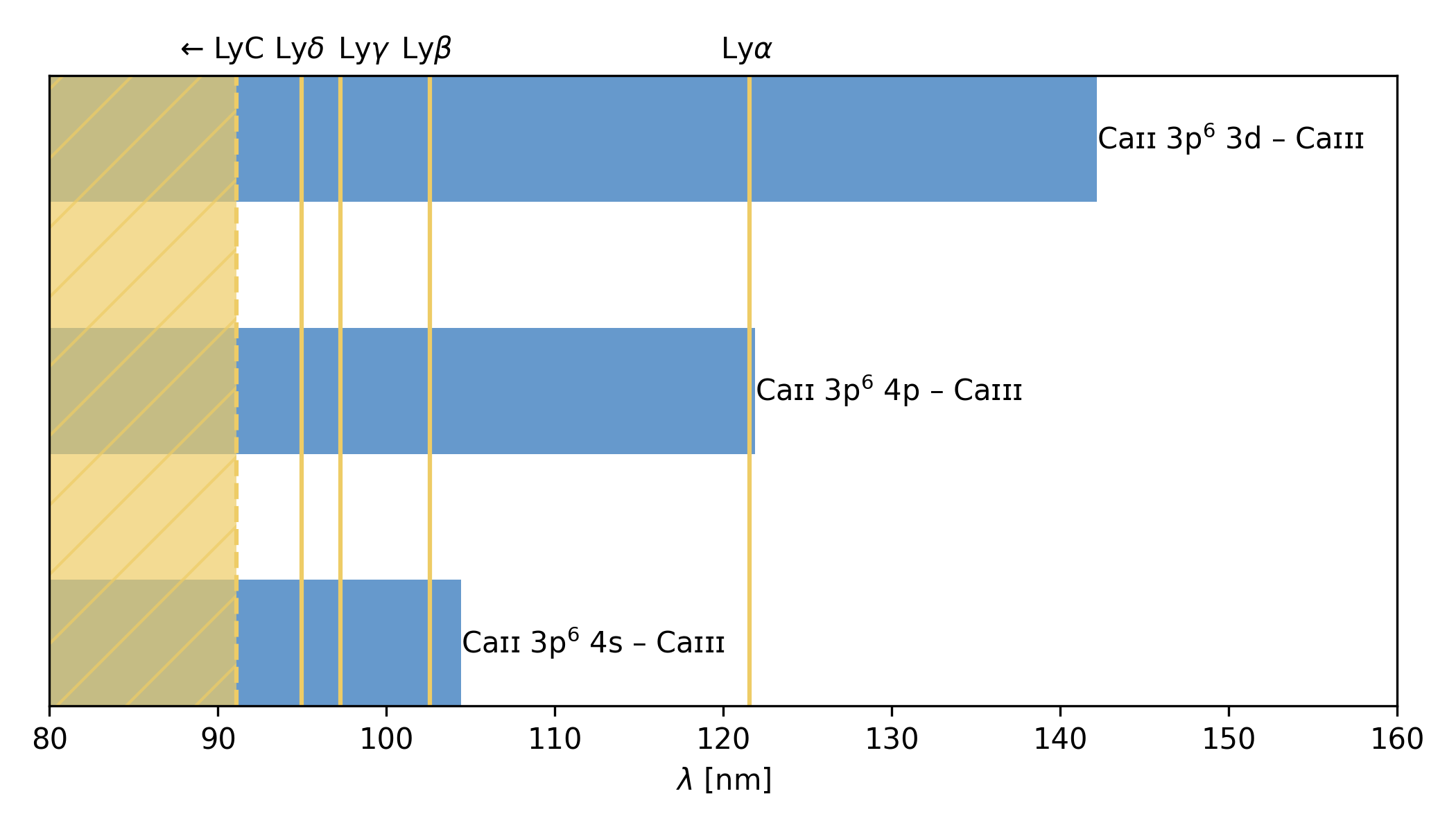
Figure 1: This diagram shows the overlap between the hydrogen Lyman lines and continuum with the Ca ii continua present in our model. Both the Ca ii 3p⁶ 4p and 3p⁶ 3d levels contain two sub-levels with close to identical continuum edges.

3 Changes to line profiles

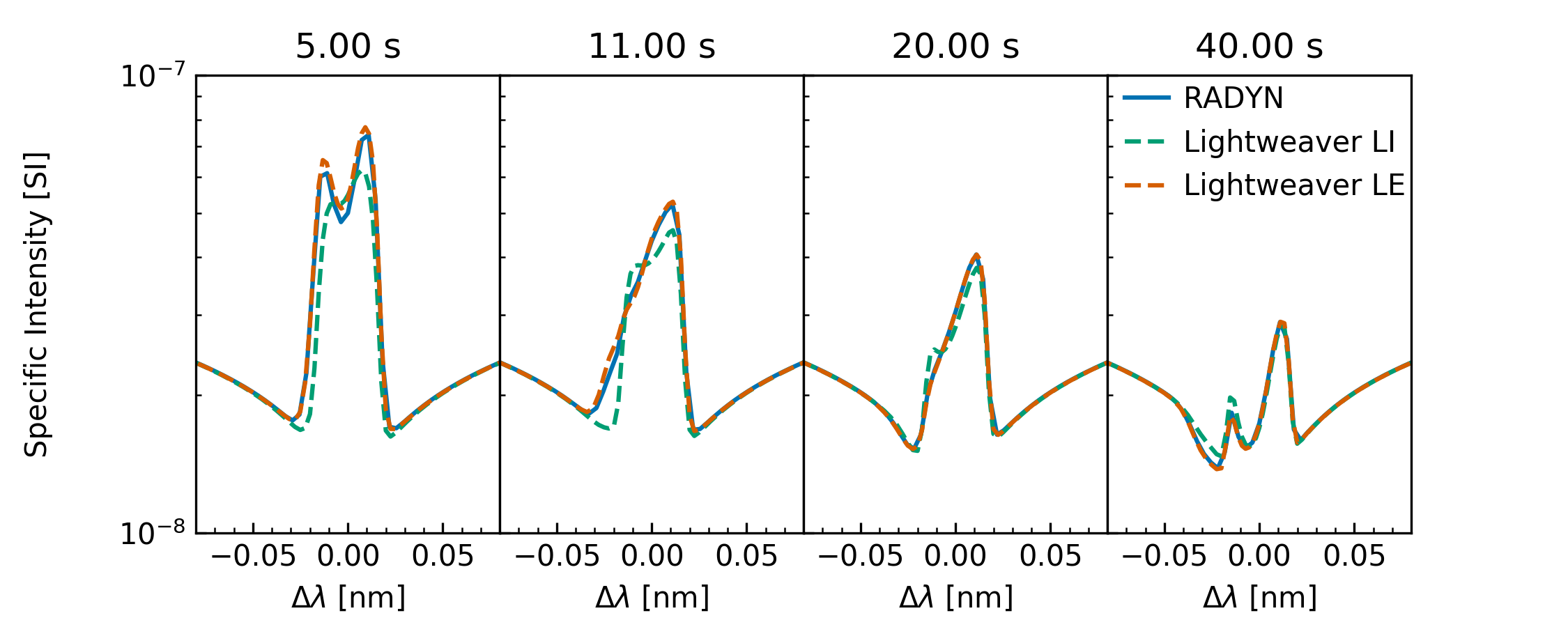
Figure 2: Comparison of Ca ii $854.2\text{\,}\mathrm{nm}$ line profiles during the F9 simulation. Specific intensity is expressed in $\mathrm{J}\text{\,}{\mathrm{s}}^{-1}\text{\,}{\mathrm{m}}^{-2}\text{\,}{\mathrm{Hz}}^{-1}\text{\,}{\mathrm{sr}}^{-1}$. Here “LI” indicates the model where photoionisation of Ca ii by the hydrogen Lyman lines is taken into account whereas “LE” excludes this effect.

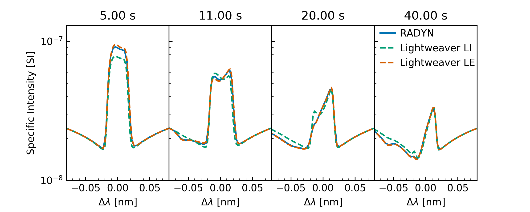
Figure 3: Comparison of Ca ii $854.2\text{\,}\mathrm{nm}$ line profiles during the F10 simulation.

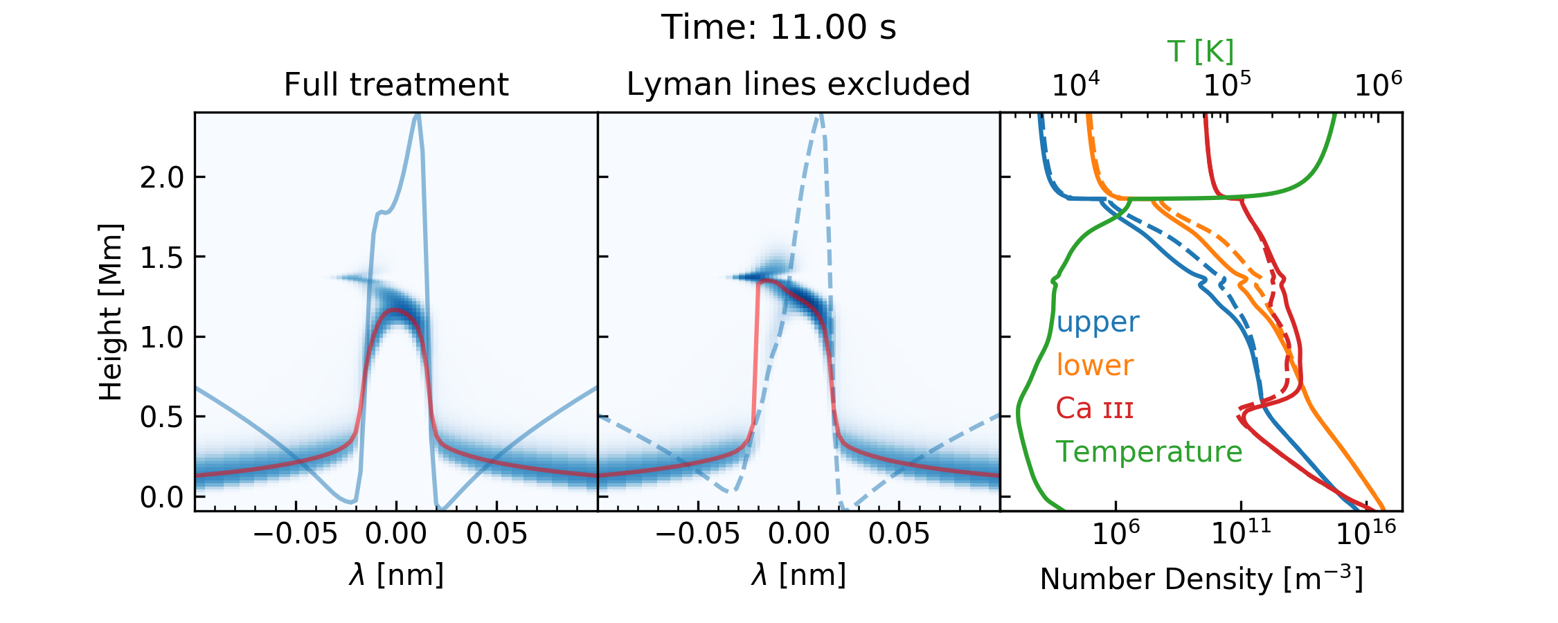
Figure 4: Contribution function and level populations for the two cases in the F9 simulation at $t=$11\text{\,}\mathrm{s}$$. The first two panels show the contribution function, emergent line profile in blue, and $\tau_{\nu}=1$ line in red. The third panel shows the temperature structure, and population density for upper and lower levels of the transition and Ca iii, where the solid lines represent the populations from the LI treatment and the dashed lines the LE treatment.

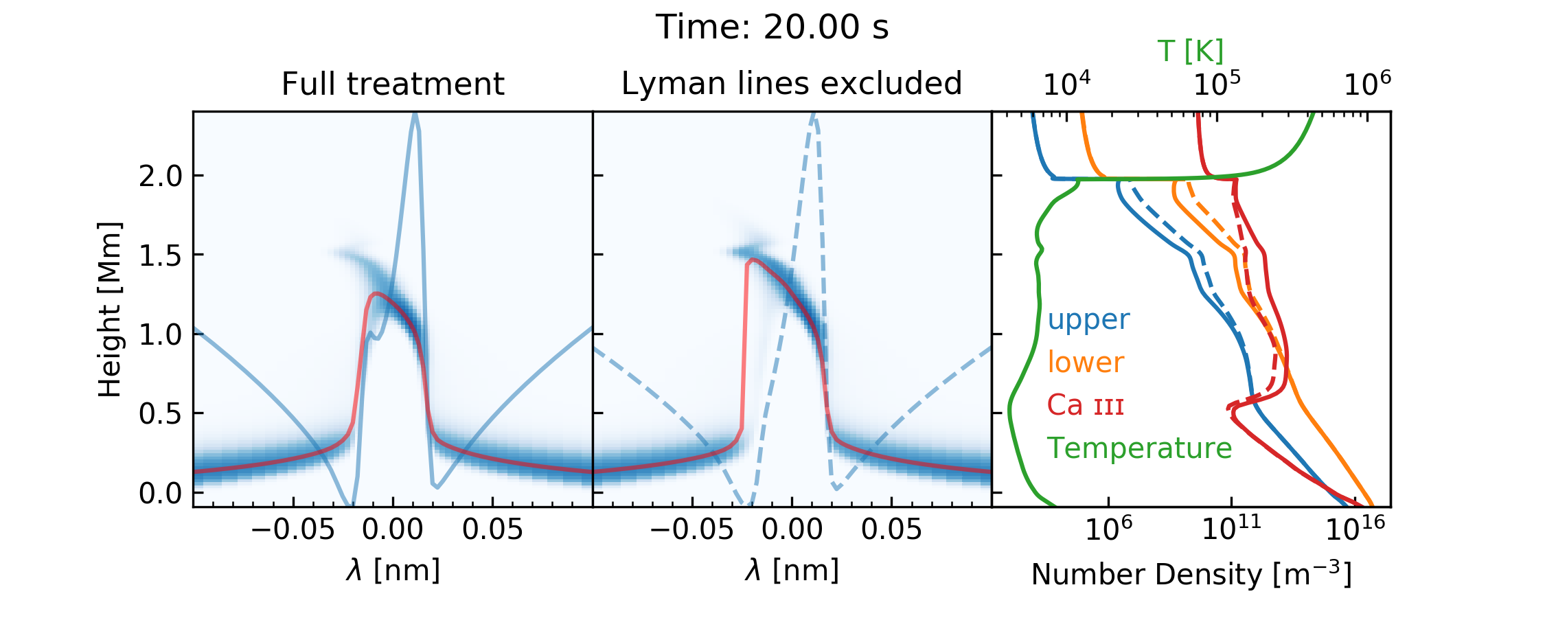
Figure 5: Contribution function and level populations for the two cases in the F9 simulation at $t=$20\text{\,}\mathrm{s}$$. The panels represent the same information as Fig. 4.

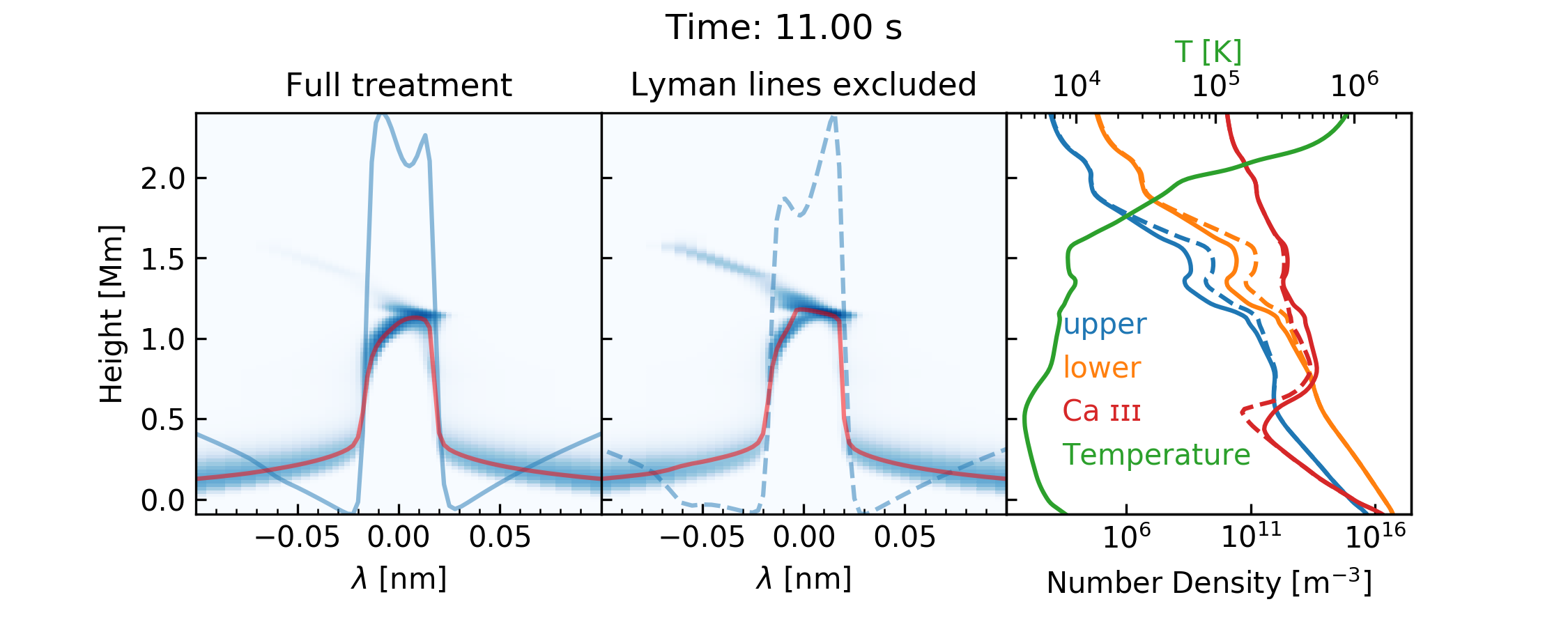
Figure 6: Contribution function and level populations for the two cases in the F10 simulation at $t=$11\text{\,}\mathrm{s}$$. The panels represent the same information as Fig. 4.

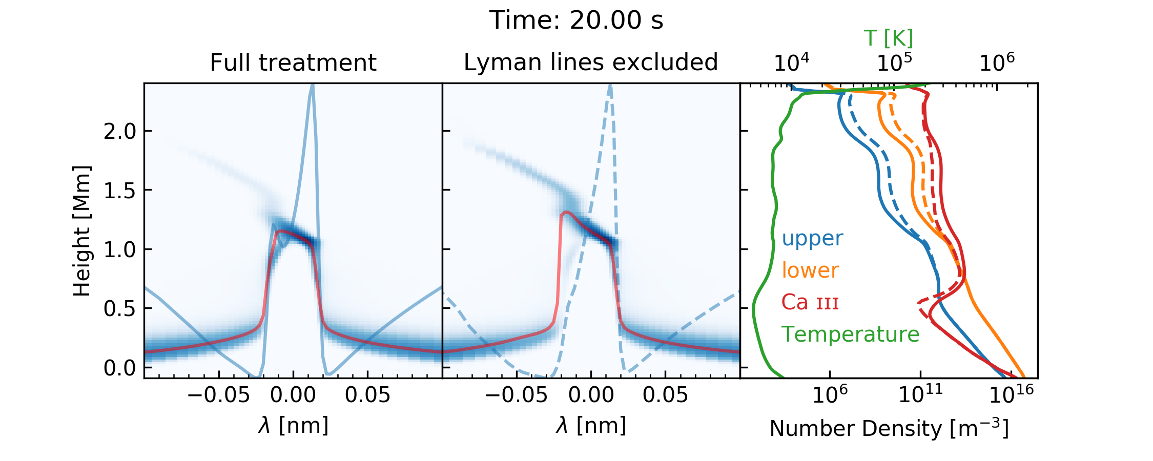
Figure 7: Contribution function and level populations for the two cases in the F10 simulation at $t=$20\text{\,}\mathrm{s}$$. The panels represent the same information as Fig. 4.

In the following we describe the simulations where the effects of the Lyman lines on Ca ii are included as Lyman inclusive (LI), and the others as Lyman exclusive (LE).

In Figs. 2 and 3 we show the Ca ii $854.2\text{\,}\mathrm{nm}$ line profile at $5$, $11$, $20$ and $40\text{\,}\mathrm{s}$ since the start of the heating for both of the simulations considered, compared against the output from the RADYN simulations. We see that the intensity from the LE model disagrees with the RADYN output by only a few percent, and the shapes remain extremely consistent, giving confidence in the Lightweaver framework. On the other hand, the line profiles produced by the LI model differ remarkably from those produced by RADYN.

For the F9 simulation shown in Fig. 2, the full LI treatment produces a narrower, less intense, double-peaked line profile, whilst the LE treatment produces a much more variable line profile, starting off sharply double-peaked, and becoming singly-peaked in the decay phase (between $11$ and $20\text{\,}\mathrm{s}$).

For the F10 simulation shown in Fig. 3, we note that during flare heating the peak intensity is substantially reduced in the LI treatment ($t=$5\text{\,}\mathrm{s}$$). At $t=$11\text{\,}\mathrm{s}$$ the asymmetry between the two peaks is reversed in the LI and LE treatments, and at $t=$20\text{\,}\mathrm{s}$$ there is a secondary peak in the violet side of the line profile in the LI case that is not present in the LE treatment. At later times there are also dips to lower intensity in the violet wing of the LE case, which evolve in shape over this cooling phase.

Due to the different line asymmetries and presence of extra peaks, we consider that the differences are most stark for the $t=11$ and $t=$20\text{\,}\mathrm{s}$$ timeslices in these simulations. Looking at the level populations for these in the right-hand panels of Figs. 4-7 we see that the LE and LI models have arrived at different populations for the upper and lower levels of Ca ii $854.2\text{\,}\mathrm{nm}$. The contribution functions, shown in the left-hand panels of Figs. 4-7, also differ significantly, leading not only to different line profiles, but to a different theoretical interpretation of where the emergent line profile is formed. In the LE models there is a contribution to the violet wing of the line present around $1.5\text{\,}\mathrm{Mm}$ that is much less significant in the LI treatment. We suggest that this occurs due to the lower population of levels involved in the formation of Ca ii $854.2\text{\,}\mathrm{nm}$ at this height, primarily due to the photoionisation of Ca ii to Ca iii in this region from Lyman lines formed in the transition region. This in turn reduces the local opacity in an area that would otherwise, due to local plasma temperature, be expected to be optically thick. This interpretation is supported by the change in the $\tau_{\nu}=1$ line present in the contribution function figures. It is also interesting to note the large variation in Ca iii populations in the F10 simulation around the temperature minimum region, much deeper than where the cores of any of the Ca ii lines form, likely due to photoionisation from the upper chromosphere and transition region.

4 Changes to radiative losses

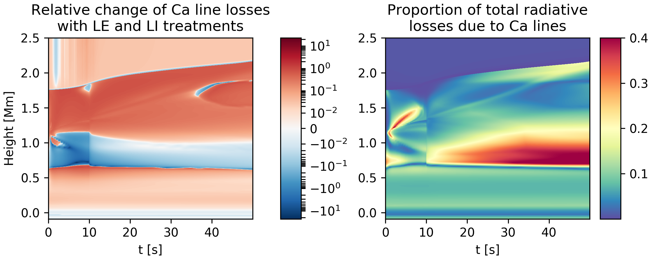
Figure 8: These panels show the time-evolution of the calcium losses in the F9 simulation. The left-hand panel shows the absolute relative change in losses due to calcium lines between the LI and LE models. The right-hand panel indicates the proportion of the total radiative losses due to calcium lines.

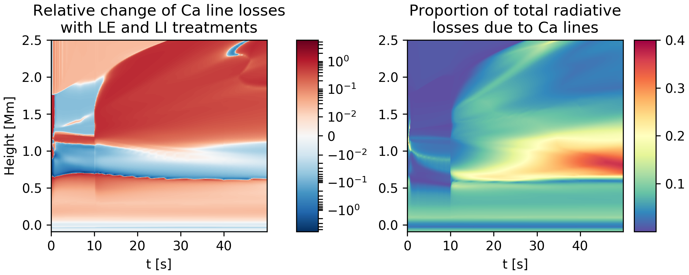
Figure 9: These panels show the time-evolution of the calcium losses in the F10 simulation. The left-hand panel shows the absolute relative change in losses due to calcium lines between the LI and LE models. The right-hand panel indicates the proportion of the total radiative losses due to calcium lines.

Figs. 8 and 9 show the variation between the two calcium treatments in both simulations, as well as the proportion of the radiative losses that the calcium lines represent in the RADYN simulation. The fine band where there is a large difference between the two treatments is around the temperature minimum region of the original simulation, and should remain relatively unimportant for the formation of this line. The left-hand panel is computed as

$$\frac{\sum_{i\in\mathcal{C}}|\mathrm{loss}_{i,\,\mathrm{LE}}|-\sum_{i\in\mathcal{C}}|\mathrm{loss}_{i,\,\mathrm{LI}}|}{\sum_{i\in\mathcal{C}}|\mathrm{loss}_{i,\,\mathrm{LE}}|},$$ (1)

where $\mathcal{C}$ is the set of calcium lines in our model, $\mathrm{loss}_{i}$ is the volumetric radiative loss ($\mathrm{W}\text{\,}{\mathrm{m}}^{-3}$), and the right-hand panel is computed as

$$\frac{\sum_{i\in\mathcal{C}}|\mathrm{loss}_{i,\,\mathrm{RADYN}}|}{\sum_{j}|\mathrm{loss}_{j,\,\mathrm{RADYN}}|},$$ (2)

i.e. the fraction of the so-called detailed radiative losses due to calcium lines in RADYN. Here, the term “detailed radiative losses” describes the losses that are computed from the full NLTE treatment (i.e. lines and continua from hydrogen, helium, and calcium). The absolute value is used inside the summations here as many of the terms inside the summation are otherwise of opposing sign and the denominator terms may be significantly smaller than the numerator, making it hard to evaluate the magnitude of these effects.

In the less energetic simulation there is a significant difference in the calcium losses between the two treatments during heating (as can be expected from the large variation in line profiles). There is also a large effect present in the F10 simulation, in a narrower band, centred on $\sim$$1.2\text{\,}\mathrm{Mm}$ where the core of the line forms.

In both cases the region where the two treatments agree quite well ($0.6$ to $1.1\text{\,}\mathrm{Mm}$), is also the region where calcium losses are maximal for most of the simulation. In the $1$ to $2\text{\,}\mathrm{Mm}$ region, the calcium lines typically represent 5-20% of the total detailed losses, and the relative change of radiative loss between the two calcium treatments is mostly in excess of 50%.

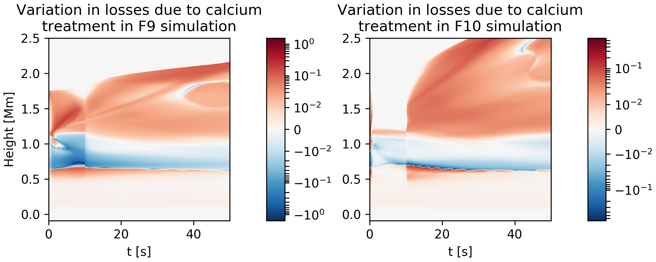
Figure 10: The absolute relative change of the detailed radiative losses, based on the change between the LE and the LI treatments (i.e. the product of the left- and right-hand panels of Figs 8 and 9) for both the F9 and F10 simulations.

The effect on the total detailed radiative losses in the simulation can be approximately described by the product of the left- and right-hand panels in Figs. 8 and 9. These are plotted in Fig. 10, and there is up to a 15% difference in the detailed radiative losses throughout the majority of the chromosphere. The time-averaged variation in radiative losses in the chromosphere is smaller in the F10 simulation than the F9, although they remain of the same order of magnitude, and this is likely due to the calcium accounting for a smaller portion of the total radiative losses in the F10 case. It is therefore reasonable to suggest that a complete RADYN-style simulation using an LI treatment could see changes in the chromospheric energy balance of around 10-15% and could therefore present different atmospheric evolution, beyond the shape and interpretation of the calcium line profiles.

5 Discussion and Conclusions

We have shown that the inclusion of the radiation field from the hydrogen Lyman lines in the calculation of the calcium populations substantially change both the emergent calcium line profiles, and the formation regions of these lines. Additionally, these effects can change the energy balance in the upper chromosphere by up to 15% in the simulations investigated here, and could therefore modify the atmospheric evolution, further increasing the change in the emergent line profiles. It is therefore important to consider these effects and analyse them further in simulations including the energy balance from the Lyman line inclusive treatment in a self-consistent way.

Whilst not presented here, we have additionally confirmed these results using the flare simulation presented in Kašparová et al. (2019). The FLARIX results were inserted into a Lightweaver model and similar relative differences between LI and LE for the Ca ii $854.2\text{\,}\mathrm{nm}$ line were found. Both time-dependent and statistical equilibrium solutions from RADYN and FLARIX snapshots were computed for this simulation and the others presented above. Little difference was found for the Ca ii line profiles, showing that the non-equilibrium ionisation of Ca ii plays a marginal role here, and that of photoionisation by the hydrogen Lyman lines appears significantly greater. There is no clear correlation between the changes to these spectral lines and the increasing flux between the F9 and F10 models, in both cases the effects are significant and appear likely to remain so as the energy input increases further.

For the simulations presented here we have also performed a cursory investigation of these effects on the Ca ii H resonance line, and found that they are less significant than on Ca ii $854.2\text{\,}\mathrm{nm}$, settling back to the LE solution much faster after the beam heating ends. This may be due to the lack of overlap between Ly$\alpha$ and the Ca ii resonance continuum, but further investigation is needed. We note that similar effects will also occur with the photoionisation of Mg ii by the Lyman continuum, but as the edge of the Mg ii resonance continuum lies at $82.46\text{\,}\mathrm{nm}$, only the Lyman continuum can contribute and the effects of the Lyman lines investigated here only apply to subordinate continua.

Acknowledgments

C.M.J.O. acknowledges support from the UK Research and Innovation’s Science and Technology Facilities Council (STFC) doctoral training grant ST/R504750/1. P.H. and J.K. were supported by grant 19-09489S (GACR) and project RVO:67985815. L.F. acknowledges support from UK Research and Innovation’s Science and Technology Facilities Council under grant award number ST/T000422/1. This research arose from discussions held at and around a meeting of the International Space Science Institute (ISSI) team: “Interrogating Field-Aligned Solar Flare Models: Comparing, Contrasting and Improving” organised by G.S. Kerr and V. Polito and we would like to thank ISSI-Bern for supporting this team.

Data Availability

The data underlying this article is available in Zenodo at https://dx.doi.org/10.5281/zenodo.4727772. The Lightweaver framework (v0.5.0) is available in Zenodo at https://dx.doi.org/10.5281/zenodo.4549258, and the scripts associated with the model presented here is available in Zenodo at https://doi.org/10.5281/zenodo.4757502 (v1.1.0).

References

- Abbett & Hawley (1999) Abbett W. P., Hawley S. L., 1999, The Astrophysical Journal, 521, 906
- Allred et al. (2005) Allred J. C., Hawley S. L., Abbett W. P., Carlsson M., 2005, The Astrophysical Journal, 630, 573
- Allred et al. (2015) Allred J. C., Kowalski A. F., Carlsson M., 2015, The Astrophysical Journal, 809, 104
- Bjørgen et al. (2019) Bjørgen J. P., Leenaarts J., Rempel M., Cheung M. C. M., Danilovic S., Rodríguez J. d. l. C., Sukhorukov A. V., 2019, Astronomy & Astrophysics, 631, A33
- Bradshaw & Cargill (2013) Bradshaw S. J., Cargill P. J., 2013, The Astrophysical Journal, 770, 12
- Bradshaw & Mason (2003) Bradshaw S. J., Mason H. E., 2003, Astronomy & Astrophysics, 401, 699
- Brown et al. (2018) Brown S. A., Fletcher L., Kerr G. S., Labrosse N., Kowalski A. F., Rodríguez J. D. L. C., 2018, The Astrophysical Journal, 862, 59
- Carlsson & Stein (1992) Carlsson M., Stein R. F., 1992, The Astrophysical Journal, 397, L59
- Carlsson & Stein (1997) Carlsson M., Stein R. F., 1997, The Astrophysical Journal, 481, 500
- Centeno (2018) Centeno R., 2018, The Astrophysical Journal, 866, 89
- Curtis et al. (1974) Curtis A. R., Powell M. J., Reid J. K., 1974, IMA Journal of Applied Mathematics (Institute of Mathematics and Its Applications), 13, 117
- De Feiter & Švestka (1975) De Feiter L. D., Švestka Z., 1975, Solar Physics, 41, 415
- Emslie (1978) Emslie A. G., 1978, The Astrophysical Journal, 224, 241
- Fang et al. (1993) Fang C., Henoux J., Gan W., 1993, Astronomy & Astrophysics, 274, 917
- Gouttebroze & Heinzel (2002) Gouttebroze P., Heinzel P., 2002, Astronomy & Astrophysics, 385, 273
- Heinzel et al. (2015) Heinzel P., Kašparová J., Varady M., Karlický M., Moravec Z., 2015, Proceedings of the International Astronomical Union, 11, 233
- Hong et al. (2019) Hong J., Li Y., Ding M. D., Carlsson M., 2019, The Astrophysical Journal, 879, 128
- Ishizawa (1971) Ishizawa T., 1971, Publications of the Astronomical Society of Japan, 23, 75
- Judge (2017) Judge P. G., 2017, The Astrophysical Journal, 851, 5
- Kašparová et al. (2003) Kašparová J., Heinzel P., Varady M., Karlický M., 2003, in Hubeny I., Mihalas D., Werner K., eds, Stellar Atmosphere Modeling, ASP Conference Proceedings, Vol. 288. Astronomical Society of the Pacific, San Francisco, p. 544, https://ui.adsabs.harvard.edu/abs/2003ASPC..288..544K
- Kašparová et al. (2019) Kašparová J., Carlsson M., Varady M., Heinzel P., 2019, in Werner K., Stehlé C., Rauch T., Lanz T. M., eds, Radiative Signatures From the Cosmos, ASP Conference Serries Vol 519. Astronomical Society of the Pacific, San Francisco, p. 141, https://ui.adsabs.harvard.edu/abs/2019ASPC..519..141K
- Kerr et al. (2016) Kerr G. S., Fletcher L., Russell A. J. B., Allred J. C., 2016, The Astrophysical Journal, 827, 101
- Kerr et al. (2019a) Kerr G. S., Allred J. C., Carlsson M., 2019a, The Astrophysical Journal, 883, 57
- Kerr et al. (2019b) Kerr G. S., Carlsson M., Allred J. C., 2019b, The Astrophysical Journal, 885, 119
- Kuridze et al. (2015) Kuridze D., et al., 2015, The Astrophysical Journal, 813, 125
- Kuridze et al. (2018) Kuridze D., Henriques V. M. J., Mathioudakis M., van der Voort L. R., de la Cruz Rodríguez J., Carlsson M., 2018, The Astrophysical Journal, 860, 10
- Osborne & Milić (2021) Osborne C. M. J., Milić I., 2021, arXiv e-prints, p. arXiv:2107.00475
- Osborne et al. (2019) Osborne C. M. J., Armstrong J. A., Fletcher L., 2019, The Astrophysical Journal, 873, 128
- Pereira & Uitenbroek (2015) Pereira T. M. D., Uitenbroek H., 2015, Astronomy & Astrophysics, 574, A3
- Reep et al. (2019) Reep J. W., Bradshaw S. J., Crump N. A., Warren H. P., 2019, The Astrophysical Journal, 871, 18
- Rimmele et al. (2020) Rimmele T. R., et al., 2020, Solar Physics, 295, 172
- Rubio Da Costa et al. (2009) Rubio Da Costa F., Fletcher L., Labrosse N., Zuccarello F., 2009, Astronomy & Astrophysics, 507, 1005
- Rubio da Costa et al. (2016) Rubio da Costa F., Kleint L., Petrosian V., Liu W., Allred J. C., 2016, The Astrophysical Journal, 827, 38
- Rybicki & Hummer (1992) Rybicki G. B., Hummer D. G., 1992, Astronomy & Astrophysics, 262, 209
- Saint-Hilaire et al. (2008) Saint-Hilaire P., Krucker S., Lin R. P., 2008, Solar Physics, 250, 53
- Scharmer et al. (2008) Scharmer G. B., et al., 2008, The Astrophysical Journal, 689, L69
- Strang (1968) Strang G., 1968, SIAM Journal on Numerical Analysis, 5, 506
- Sui et al. (2007) Sui L., Holman G. D., Dennis B. R., 2007, The Astrophysical Journal, 670, 862
- Uitenbroek (2001) Uitenbroek H., 2001, The Astrophysical Journal, 557, 389
- Varady et al. (2010) Varady M., Kašparová J., Moravec Z., Heinzel P., Karlický M., 2010, IEEE Transactions on Plasma Science, 38, 2249
- Vernazza et al. (1981) Vernazza J. E., Avrett E. H., Loeser R., 1981, The Astrophysical Journal Supplement Series, 45, 635
- de la Cruz Rodríguez & Piskunov (2013) de la Cruz Rodríguez J., Piskunov N., 2013, The Astrophysical Journal, 764, 33