Effects of strain stiffening and electrostriction on tunable elastic waves
in compressible dielectric elastomer laminates

Abstract

This paper presents an electromechanical analysis of the nonlinear static response and the superimposed small-amplitude wave characteristics in an infinite periodic compressible dielectric elastomer (DE) laminate subjected to electrostatic excitations and prestress in the thickness direction. The enriched Gent material model is employed to account for the effects of strain stiffening and electrostriction of the DE laminate. The theory of nonlinear electroelasticity and related linearized incremental theory are exploited to derive the governing equations of nonlinear response and the dispersion relations of incremental shear and longitudinal waves. Numerical results reveal that the snap-through instability of a Gent DE laminate resulting from geometrical and material nonlinearities can be used to achieve a sharp transition in the position and width of wave band gaps. Furthermore, the influence of material properties (including Gent constants, the second strain invariant and electrostrictive parameters) and that of prestress on the snap-through instability and the electrostatic tunability of band gaps for both shear and longitudinal waves are discussed in detail. The electrostrictive effect and prestress are beneficial to stabilizing the periodic DE laminate. Depending on whether the snap-through instability occurs or not, a continuous variation or a sharp transition in wave band gaps can be realized by varying the electric stimuli. Our numerical findings are expected to provide a solid guidance for the design and manufacture of soft DE wave devices with tunable band structures.

1 Introduction

Dielectric elastomers (DEs) are one type of smart soft materials that can deform and change their physical properties dramatically in response to an external electric stimulus. Owing to their fascinating characters, such as large controllable deformation, light weight, high fracture toughness, and high sensitivity, DEs have been widely used in various engineering applications ranging from energy harvesters, soft robots and sensing devices to tunable resonators (Koh et al., 2010; Huang et al., 2013; Viry et al., 2014; Li et al., 2017b; Lu et al., 2013, 2015; Sugimoto et al., 2013; Yu et al., 2017; Chen et al., 2019a). In particular, Lu et al. (2013) designed and investigated experimentally a DE absorber with a back cavity, and achieved broadband frequency absorptions of noise. The same authors (Lu et al., 2015) developed a new type of duct silencer made of DE actuators whose acoustic characteristics can be actively tuned by voltage. A semicylindrical push-pull acoustic transducer composed of DE films was proposed by Sugimoto et al. (2013) for the supression of harmonic distortion. Yu et al. (2017) realized the broadband sound attenuation in a novel acoustic metamaterial consisting of an array of DE resonators, which can be tuned by either electric or mechanical biasing fields. Recently, a comprehensive electromechanical characterization of different DE materials was conducted experimentally by Chen et al. (2019a) to promote practical applications of DE actuators and generators.

It is well-known that large deformations induced by the electric field will significantly affect the electromechanical properties of DEs, which may provide an effective approach to manipulating the acoustic/elastic waves in these soft matters. In recent years, many efforts have been devoted to studying small-amplitude wave propagation characteristics in DEs under the application of electric and mechanical biasing fields following the theory of nonlinear electroelasticity and its associated linearized incremental theory developed by Dorfmann and Ogden (2005, 2010). For example, Dorfmann and Ogden (2010) investigated the propagation of Rayleigh-type surface waves superimposed on a finitely deformed electroactive (EA) half-space. The longitudinal axisymmetric waves propagating in solid and hollow DE cylinders under combined action of electric and mechanical loadings were explored by Chen and Dai (2012) and Shmuel and deBotton (2013), respectively. Then, Shmuel (2015) discussed the possibility to exploit the applied voltage to manipulate torsional elastic waves in DE tubes. Adopting proper displacement functions, the non-axisymmetric wave motions in an infinite incompressible soft EA hollow cylinder with uniform biasing fields were studied by Su et al. (2016). For soft EA tubes under inhomogeneous electromechanical biasing fields, Wu et al. (2017) employed the State Space Method to analyze the guided circumferential waves propagation and pointed out that it is feasible to design self-sensing EA actuator and conduct ultrasonic non-destructive detection of soft EA structures via the circumferential waves. Recently, an experimental apparatus was designed by Ziser and Shmuel (2017) to excite and measure elastic waves in a DE film, and the experimental results demonstrated that the wave velocity of the fundamental flexural wave could be slowed down under voltage.

Most of the existing works on wave propagation adopt the ideal dielectric model with constant dielectric permittivity to characterize the soft EA materials. In fact, the electrostrictive effect describing the deformation-dependent permittivity has been experimentally observed (Wissler and Mazza, 2007; Li et al., 2011) and plays an important role in the electromechanical analysis of DEs. Zhao and Suo (2008) proposed a thermodynamic electrostrictive model for DEs and pointed out that the electrostrictive effect may become pronounced at large deformations and should not be neglected. Utilizing the enriched DE model, Gei et al. (2014) discussed the role of electrostriction on the stability of a homogeneous DE actuator and made a conclusion that electrostriction has a trend to stabilizing the DE actuator. Liu et al. (2015) developed a theoretical material model coupling electrostriction with polarization, and proved that the stability of DE/carbon nanotube composites can be affected significantly by the electrostrictive effect. Based on the Hessian matrix method, Su et al. (2018) presented a theoretical analysis of parameter optimization (including the strain-stiffening and electrostrictive parameters) to achieve giant deformations of an incompressible DE plate. As regards the investigation on elastic waves, Galich and Rudykh (2016) found that whether accounting for the electrostrictive effect into the material model or not evidently influences shear and pressure bulk wave propagation behaviors in compressible DEs subjected to an electrostatic field. Although the existing experimental results of the electrostrictive effect are still contradictory, there is no definite conclusion yet. For example, Chen et al. (2019a) argued that the dielectric permittivity parameters for three DE materials are deformation-independent, but they also pointed out that there exist experimental errors and the measurement of electrostrictive parameters also depends on the electrode and DE type, DE size and shape, interfacial integrity, edge effects and other factors. Thus, the electrostrictive effect may appear in different DE materials and it should be of practical value to study its effect on the nonlinear response and wave propagation behaviors in DE structures.

Since the concept of phononic crystals (i.e. PCs, which are intrinsically periodic composites) was first proposed in the 1990s (Kushwaha et al., 1993), their unique properties have attracted intensive research interests and provided new avenues for the manipulation of acoustic/elastic waves. Due to the Bragg scattering mechanism or the locally resonant mechanism (Liu et al., 2000), band gap is the most important feature of PCs, which corresponds to the frequency range where waves are forbidden to propagate in media (Li and Wang, 2012; Yuan et al., 2019; Wang et al., 2020). Many acoustic devices with desired superior functions have been designed on the foundation of band gaps (Soukiassian et al., 2007; Liang et al., 2009; Gao et al., 2017; Ma et al., 2018; Huang et al., 2018; Gao et al., 2018; Chen et al., 2019b). However, once the structures are fabricated with specified geometrical and material parameters, the operating frequencies of most traditional PCs are generally fixed. Therefore, in order to realize real-time control of waves, a large number of researches have been carried out to acquire high-performance PCs with broad tunable band gaps. For example, in a two-dimensional PC composed of air and quartz, Huang and Wu (2005) found that the band structure of both bulk modes and surface modes can be tuned by the temperature variation. Yang et al. (2014) showed experimentally that the band gap of a magneto-mechanical PC is highly sensitive to a small magnetic field due to the magnetic torque effect on the coupling between Bragg scattering and local resonant modes. Lian et al. (2016) proposed a piezoelectric PC connected with resonant shunting circuits and indicated that both central frequency and bandwidth of the locally resonant band gaps decrease with the increase of resistance and inductance. A soft membrane-type acoustic metamaterial was designed by Zhou et al. (2018), and its band gap strongly depends on the applied pre-stretch when choosing Gent material model. By employing periodic electrical boundary conditions, an innovative design to generate actively tunable topologically protected interface mode in a homogeneous piezoelectric rod system was proposed by Zhou et al. (2020). Matar et al. (2013) and Wang et al. (2020) provided literature overview on tunable PCs by diverse tuning methods and demonstrated a brilliant prospect in optional manipulation of waves via tunable PCs. More recently, the research status, design principles, future development and challenges were reviewed by Bertoldi et al. (2017) for soft or flexible mechanical PCs and metamaterials (MMs).

Among the researches on tunable PCs, some studies have been conducted to use large deformation and electric stimuli to tune wave propagation behaviors in PCs composed of soft EA materials. Yang and Chen (2007) carried out the first piece of work to explore the electro-mechanical coupling effects in soft DE PCs, and achieved the tunable band gaps in a two-dimensional PCs consisting of hollow DE cylinders immersed in an air background. A pre-stretched DE membrane-type waveguide was proposed by Gei et al. (2010) for the purpose of tuning bandgap position at will. Shmuel and deBotton (2012) investigated the incremental thickness-shear waves propagating in a DE laminate composed of two alternating neo-Hookean (N-H) phases, and analyzed the tunability of band gaps under electric biasing field. Then, Getz and Shmuel (2017) found that the band gaps of DE composite plates can be adjusted by the applied voltage and suggested its application to actively tunable waveguides and isolators. Galich and Rudykh (2017) re-checked the results in Shmuel and deBotton (2012) and a different conclusion was obtained that the band gaps of shear wave propagating in periodic Gent DE laminates may be widened and lifted up via the applied electric stimuli, while the band gaps keep unchanged for the N-H material model. Recently, Zhu et al. (2018) obtained the dispersion relation and transmission behaviors of shear horizontal wave propagating in the periodic DE laminate and demonstrated the tunable effect of external electric stimuli on shear wave band gaps. In addition, by adopting a genetic algorithm approach, Bortot et al. (2018) utilized the topological optimization to maximize the band-gap width of anti-plane shear waves propagating in DE fiber composites.

Nevertheless, all of the above-mentioned works take no account of the instabilities that commonly occur in soft EA structures. It is worth noting that different kinds of instabilities can be used to enhance the electrostatic manipulability for acoustic/elastic waves in soft EA PCs, which is an interesting topic and has received some attention. Bortot and Shmuel (2017) made use of the plane wave expansion method to explore the electrostatic tunability of an array of DE tubes surrounded by air, and showed that the snap-through instability can be used to achieve an abrupt transition in band gaps. Recently, Wu et al. (2018) investigated the longitudinal waves propagating in a one-dimensional PC cylinders tuned by axial force and voltage, and obtained a sudden and enormous change in the band gaps through the snap-through transition emerging only in the Gent DE materials. Using the finite-element-based numerical simulations, Jandron and Henann (2018) presented the possibility to harness electromechanical pull-in instability and macroscopic instability to achieve enhanced electrical tunability of waves in soft DE composites. The snap-through instability induced by both electric voltage and internal pressure was also exploited by Mao et al. (2019) to realize the resonant frequency jump of soft EA balloons.

The primary objective of the present investigation is to shed light on the effects of material properties (including strain stiffening and electrostriction) and external loadings (including electric stimuli and prestress) on the nonlinear response and the superimposed shear and longitudinal waves in a periodic two-phase compressible DE laminate. The research motivations are the following four important aspects: (1) The material compressibility needs to be considered when analyzing the longitudinal wave propagation; (2) How the snap-through instability due to the strain-stiffening effect influences the static and dynamic behaviors of periodic DE laminate; (3) How the second strain invariant affects the nonlinear static response and wave propagation in the DE laminate; (4) To what extent of the electric stimuli, the electrostrictive effect will become significant.

This paper is outlined as follows. A brief summary of basic formulations of the nonlinear electroelasticity theory and related linearized incremental theory is described in Section 2. The nonlinear deformation of a periodic compressible DE laminate is considered in Section 3 for the enriched Gent material model. Combining the transfer matrix method with the Bloch-Floquet theorem, Section 4 derives the dispersion relations for the incremental shear and longitudinal waves. Then numerical discussions in Section 5 elucidate the effects of strain stiffening, the second strain invariant, electrostriction and prestress on the nonlinear deformation and the band structures of periodic DE laminate subjected to the electric stimuli. Some conclusions are finally made in Section 6.

2 Preliminary formulations

This section briefly reviews the general theory of nonlinear electroelasticity and the associated linearized incremental theory. Interested readers are referred to the papers of Dorfmann and Ogden (2005, 2006, 2010) and the monograph by Dorfmann and Ogden (2014) for more detailed discussions about the basic ideas.

2.1 Nonlinear electroelasticity theory

Consider a deformable electroelastic body that occupies a region ${{\mathcal{B}}_{r}}$ in the Euclidean space with the boundary $\partial{{\mathcal{B}}_{r}}$ and the outward unit normal $\mathbf{N}$ in the undeformed ‘reference configuration’ at time ${{t}_{0}}$. An arbitrary material point in this state is labelled by its position vector $\mathbf{X}$. The body moves to a region ${{\mathcal{B}}_{t}}$ with the boundary $\partial{{\mathcal{B}}_{t}}$ and the outward unit normal $\mathbf{n}$ at time $t$, if subjected to a motion $\mathbf{x}=\bm{\chi}\text{(}\mathbf{X},t\text{)}$, where $\bm{\chi}$ is a vector field function with a sufficiently regular property and $\mathbf{x}$ is the new location of the material point associated with $\mathbf{X}$ in the ‘current configuration’. The deformation gradient tensor is defined as $\mathbf{F}=\text{Grad }\bm{\chi}$, where Grad is the gradient operator with respect to ${{\mathcal{B}}_{r}}$, and ${{\mathbf{F}}_{i\alpha}}=\partial{{x}_{i}}/\partial{{X}_{\alpha}}$ in Cartesian components. Note that Greek and Roman indices are associated with ${{\mathcal{B}}_{r}}$ and ${{\mathcal{B}}_{t}}$, respectively. We will adopt the summation convention for repeated indices. The relations between the infinitesimal line element $\text{d}\mathbf{X}$, surface element $\text{d}A$ and volume element $\text{d}V$ in ${{\mathcal{B}}_{r}}$ and those in ${{\mathcal{B}}_{t}}$ are connected by $\text{d}\mathbf{x}=\mathbf{F}\text{d}\mathbf{X}$, the well-known Nanson’s formula $\mathbf{n}\text{d}a=J{{\mathbf{F}}^{-\text{T}}}\mathbf{N}\text{d}A$ and $\text{d}v=J\text{d}V$, respectively. Here the superscript ${}^{\text{T}}$ signifies the transpose of a second-order tensor if not otherwise stated and $J=\det\mathbf{F}>0$ denotes the local measure of volume change. The left and right Cauchy-Green tensors are defined as $\mathbf{b=F}{{\mathbf{F}}^{\text{T}}}$ and $\mathbf{C=}{{\mathbf{F}}^{\text{T}}}\mathbf{F}$ that will be employed as the deformation measures.

Here, under the assumption of the quasi-electrostatic approximation, Gauss’s law and Faraday’s law in the absence of free charges and currents can be read as

$${\rm{div}}{\kern 1.0pt}{\bf{D}}=0,\quad{\rm{curl}}{\kern 1.0pt}{\bf{E}}={\bf{0}},$$ (1)

where ‘curl’ and ‘div’ denote the curl and divergence operators in the current configuration ${{\mathcal{B}}_{t}}$; $\mathbf{D}$ and $\mathbf{E}$ are the electric displacement and electric field vectors in ${{\mathcal{B}}_{t}}$, respectively. In addition, in the absence of mechanical body forces, the equations of motion can be written as

$${\rm{div}}{\kern 1.0pt}{\bm{\tau}}=\rho{{\bf{x}}_{,tt}},$$ (2)

where $\bm{\mathbf{\tau}}$ is the so-called ‘total Cauchy stress tensor’ including the contribution of electric body forces, $\rho={{\rho}_{0}}{{J}^{-1}}$ is the mass density in the deformed configuration ${{\mathcal{B}}_{t}}$ (${{\rho}_{0}}$ is the initial material mass density in ${{\mathcal{B}}_{r}}$), and the subscript $t$ following a comma represents the material time derivative. The conservation of angular momentum ensures the symmetry of $\bm{\mathbf{\tau}}$.

In this paper, we will consider a periodic DE laminate that is coated with flexible electrodes on the leftmost and rightmost surfaces with equal and opposite surface free charges, as shown in Fig. 1. Then, there is no electric field in the surrounding vacuum by Gauss’s theorem. As to be shown in Subsec. 3, the electric displacement field in the DE laminate is uniformly distributed in the thickness direction. Therefore, the electric boundary conditions on $\partial{{\mathcal{B}}_{t}}$ yield

$${\bf{E}}\times{\bf{n}}=0,\quad{\rm{}}{\bf{D}}\cdot{\bf{n}}=-{\sigma_{\rm{f}}},$$ (3)

where ${{\sigma}_{\text{f}}}$ is the free surface charge density on $\partial{{\mathcal{B}}_{t}}$. Furthermore, the mechanical boundary condition can be expressed in Eulerian form as

$${\bm{\tau n}}={{\bf{t}}^{a}},$$ (4)

where ${{\mathbf{t}}^{a}}$ is the prescribed mechanical traction vector per unit area of $\partial{{\mathcal{B}}_{t}}$. For the corresponding Lagrangian counterparts of Eqs. (1)-(4), we refer to the works of Dorfmann and Ogden (2005, 2006).

According to the theory of nonlinear electroelasticity (Dorfmann and Ogden, 2006), the nonlinear constitutive relations for a compressible electroelastic material in terms of the total energy density function $\Omega(\mathbf{F},\bm{\mathcal{D}})$ per unit reference volume are given by

$${\bf{T}}=\frac{{\partial\Omega}}{{\partial{\bf{F}}}},\quad\bm{{\cal E}}=\frac{{\partial\Omega}}{{\partial\bm{{\cal D}}}},$$ (5)

where $\mathbf{T}=J{{\mathbf{F}}^{-1}}\mathbf{\bm{{\tau}}}$, $\mathcal{\bm{{\cal D}}}=J{{\mathbf{F}}^{-1}}\mathbf{D}$ and $\mathcal{\bm{{\cal E}}}={{\mathbf{F}}^{\text{T}}}\mathbf{E}$ are the ‘total nominal stress tensor’, Lagrangian electric displacement and electric field vectors, respectively. Thus, the nonlinear constitutive relations expressed by $\bm{{\tau}}$ and $\mathbf{E}$ can be derived as $\bm{{\tau}}=J^{-1}\mathbf{F}{{\partial\Omega}}/{{\partial{\bf{F}}}}$ and $\mathbf{E}={{\mathbf{F}}^{-\text{T}}}{{\partial\Omega}}/{{\partial\bm{{\cal D}}}}$. For a compressible isotropic electroelastic material, the form of $\Omega$ can be written as $\Omega=\Omega(I_{1},I_{2},I_{3},I_{4},I_{5},I_{6})$ depending on the following six invariants:

$$\begin{split}{I_{1}}&={\rm{tr}}{\bf{C}},\quad{I_{2}}=[{({\rm{tr}}{\bf{C}})^{2}}-{\rm{tr}}({{\bf{C}}^{2}})]/2,\quad{I_{3}}=\det{\bf{C}}={J^{2}},\\ {I_{4}}&={\bm{{\cal D}}}\cdot{\bm{{\cal D}}},\quad{I_{5}}={\bm{{\cal D}}}\cdot({\bf{C}}{\bm{{\cal D}}}),\quad{I_{6}}={\bm{{\cal D}}}\cdot({{\bf{C}}^{2}}{\bm{{\cal D}}}),\end{split}$$ (6)

which are substituted into Eq. (5) to yield the explicit forms of total stress tensor $\mathbf{\bm{\tau}}$ and electric field vector $\mathbf{E}$ as (Dorfmann and Ogden, 2010)

$$\begin{split}J{\bm{\tau}}&=2{\Omega_{1}}{\bf{b}}+2{\Omega_{2}}({I_{1}}{\bf{b}}-{{\bf{b}}^{2}})+2{I_{3}}{\Omega_{3}}{\bf{I}}+2{I_{3}}{\Omega_{5}}{\bf{D}}\otimes{\bf{D}}+2{I_{3}}{\Omega_{6}}({\bf{D}}\otimes{\bf{bD}}+{\bf{bD}}\otimes{\bf{D}}),\\ {\bf{E}}&=2J({\Omega_{4}}{{\bf{b}}^{-1}}{\bf{D}}+{\Omega_{5}}{\bf{D}}+{\Omega_{6}}{\bf{bD}}),\end{split}$$ (7)

where ${{\Omega}_{m}}=\partial\Omega/\partial{{I}_{m}}(m=1-6)$. We note that the last two terms of the expression for $J\mathbf{\bm{\tau}}$ in Dorfmann and Ogden (2010) contain typographical errors, which have been corrected in Eq. (7).

2.2 The linearized incremental theory

Based on the theoretical framework developed by Dorfmann and Ogden (2010), we reproduce the governing equations for time-dependent infinitesimal incremental changes in both motion $\dot{\mathbf{x}}\left(\mathbf{X},t\right)$ and electric displacement vector superimposed on a deformed soft electroelastic body with a static finite deformation $\mathbf{x}=\bm{\chi}\left(\mathbf{X}\right)$ and an electric displacement vector $\mathbf{D}\left(\mathbf{X}\right)$. A linearized incremental theory can be established by employing the perturbation method due to the infinitesimality of incremental mechanical and electrical fields. Here and thereafter a superposed dot signifies the increment in the quantities concerned.

In updated Lagrangian form, the incremental governing equations can be written as

$${\rm{div}}{\kern 1.0pt}{\dot{\bm{{\cal D}}}_{0}}=0,\quad{\rm{curl}}{\kern 1.0pt}{\dot{\bm{{\cal E}}}_{0}}=\bf{0},\quad{\rm{div}}{{\bf{\dot{T}}}_{0}}=\rho{{\bf{u}}_{,tt}},$$ (8)

where ${{\dot{\mathcal{{\bm{{\cal D}}}}}}_{0}}$, ${{\dot{\mathcal{\bm{{\cal E}}}}}_{0}}$ and ${{\mathbf{\dot{T}}}_{0}}$ are the ‘push forward’ versions of corresponding Lagrangian increments that update the reference configuration from the original unstressed configuration ${{\mathcal{B}}_{r}}$ to the initial static deformed configuration ${{\mathcal{B}}}$, the subscript 0 identifies the resulting ‘push forward’ variables, and $\mathbf{u}(\mathbf{x},t)=\dot{\mathbf{x}}\left(\mathbf{X},t\right)$ is the incremental displacement vector. For a compressible soft electroelastic material, the linearized incremental constitutive laws in terms of the increments ${{\mathbf{\dot{T}}}_{0}}$ and ${{\dot{\mathcal{{\bm{{\cal E}}}}}}_{0}}$ can be obtained from Eq. (5) and the push-forward operation as

$${{\bf{\dot{T}}}_{0}}={{\bm{{\cal A}}}_{0}}{\bf{H}}+{{\bm{{\cal M}}}_{0}}{\dot{\bm{{\cal D}}}_{0}},\quad{\rm{}}{\dot{\bm{{\cal E}}}_{0}}={\bm{{\cal M}}}_{0}^{\rm{T}}{\bf{H}}+{{\bm{{\cal R}}}_{0}}{\dot{\bm{{\cal D}}}_{0}},$$ (9)

where $\mathbf{H}=\text{grad}\mathbf{u}$ represents the incremental displacement gradient tensor with ‘grad’ being the gradient operator in ${{\mathcal{B}}}$. It should be emphasized that the superscript ${}^{\text{T}}$ in Eq. (9) denotes the transpose of a third-order tensor between the first two subscripts (that always go together) and the third subscript (i.e. ${\bm{{\cal M}}}_{0}^{\rm{T}}{\bf{H}}={{\cal M}_{0ijk}}H_{ij}$). The three instantaneous electroelastic moduli tensors ${{\bm{{\cal A}}}_{0}}$, ${{\bm{{\cal M}}}_{0}}$ and ${{\bm{{\cal R}}}_{0}}$ are given in component form by

$$\begin{split}{{\cal A}_{0piqj}}&={J^{-1}}{F_{p\alpha}}{F_{q\beta}}{{\cal A}_{\alpha i\beta j}}={{\cal A}_{0qjpi}},\quad{{\cal R}_{0ij}}=JF_{\alpha i}^{-1}F_{\beta j}^{-1}{{\cal R}_{\alpha\beta}}={{\cal R}_{0ji}},\\ {{\cal M}_{0piq}}&={F_{p\alpha}}F_{\beta q}^{-1}{{\cal M}_{\alpha i\beta}}={{\cal M}_{0ipq}},\end{split}$$ (10)

where $\bm{\mathcal{A}}$, $\bm{\mathcal{M}}$ and $\bm{\mathcal{R}}$ denote the referential electroelastic moduli associated with $\Omega(\mathbf{F},\bm{\mathcal{D}})$, with their components defined by ${{\mathcal{A}}_{\alpha i\beta j}}={{\partial}^{2}}\Omega/(\partial{{F}_{i\alpha}}\partial{{F}_{j\beta}})$, ${{\mathcal{M}}_{\alpha i\beta}}={{\partial}^{2}}\Omega/(\partial{{F}_{i\alpha}}\partial{{\mathcal{D}}_{\beta}})$ and ${{\mathcal{R}}_{\alpha\beta}}={{\partial}^{2}}\Omega/(\partial{{\mathcal{D}}_{\alpha}}\partial{{\mathcal{D}}_{\beta}})$. Moreover, the additional incremental incompressibility condition is given by

$$\mbox{div\hskip 1.0pt}\mathbf{u}=\mbox{tr\hskip 1.0pt}\mathbf{H}=0.$$ (11)

Finally, the updated Lagrangian incremental forms of electric and mechanical boundary conditions, which hold on $\partial{{\mathcal{B}}}$, will become

$${\dot{\bm{{\cal E}}}_{0}}\times{\bf{n}}=0,\quad{\dot{\bm{{\cal D}}}_{0}}\cdot{\bf{n}}=-{\dot{\sigma}_{{\rm{F0}}}},\quad{\bf{\dot{T}}}_{0}^{\rm{T}}{\bf{n}}={\bf{\dot{t}}}_{0}^{A},$$ (12)

where the electrical variables and their increments in the surrounding vacuum have been discarded, and ${{\dot{\sigma}}_{\text{F0}}}$ and $\mathbf{\dot{t}}_{0}^{A}$ are the incremental surface charge density and mechanical traction vector per unit area of $\partial{{\mathcal{B}}}$, respectively.

3 Nonlinear deformation of an infinite periodic DE laminate

Figure 1: Sketch of an infinite two-phase periodic DE laminate subjected to voltage $V$ and prestress $\tau_{33}^{0}$ in the thickness direction.

As shown in Fig. 1, we consider an infinite periodic DE laminate composed of two compressible alternating phases denoted by $a$ and $b$, with the thickness of undeformed unit cell being $H={{H}^{\left(a\right)}}+{{H}^{\left(b\right)}}$ along the ${{x}_{3}}$ direction. In the following, the physical quantities of the $p$-th ($p=a,b$) phase are indicated by the superscript ${{\left(\cdot\right)}^{\left(p\right)}}$. Geometrically, the initial volume fractions of phase $a$ and phase $b$ are ${{\nu}^{\left(a\right)}}={{H}^{\left(a\right)}}/H$ and ${{\nu}^{\left(b\right)}}={{H}^{\left(b\right)}}/H$, respectively. It is assumed that, when subjected to an electric voltage $V$ between the two mechanically negligible electrodes on the leftmost and rightmost surfaces of the laminate as well as a prestress $\tau_{33}^{0}$ along the thickness direction, each layer of the DE laminate is allowed to expand freely in the ${{x}_{1}}$ and ${{x}_{2}}$ directions. Now the length of the deformed unit cell and the thicknesses of each phase become

$$h={h^{\left(a\right)}}+{h^{\left(b\right)}},\quad{h^{\left(a\right)}}=\lambda_{3}^{\left(a\right)}{H^{\left(a\right)}},\quad{h^{\left(b\right)}}=\lambda_{3}^{\left(b\right)}{H^{\left(b\right)}},$$ (13)

where $\lambda_{3}^{\left(a\right)}$ and $\lambda_{3}^{\left(b\right)}$ are the stretch ratios of the two phases in the ${{x}_{3}}$ direction, and $h$ is the length of the unit cell in the deformed configuration. In virtue of the perfect bonding condition between the two homogeneous phases and the symmetry of the problem in the $x_{1}$-$x_{2}$ plane, we obtain the following relations

$$\lambda_{1}^{\left(a\right)}=\lambda_{2}^{\left(a\right)}=\lambda_{1}^{\left(b\right)}=\lambda_{2}^{\left(b\right)}=\lambda,$$ (14)

where $\lambda_{1}^{\left(p\right)}$ and $\lambda_{2}^{\left(p\right)}$ denote the stretch ratios of phase $p$ in the ${{x}_{1}}$ and ${{x}_{2}}$ directions, respectively. Therefore, the deformation gradient tensor of phase $p$ can be expressed as ${{\mathbf{F}}^{\left(p\right)}}=\text{diag}[\lambda,\lambda,\lambda_{3}^{\left(p\right)}]$ with its components to be solved by boundary conditions. Since the voltage is applied along the ${{x}_{3}}$ direction, it can be derived that $D_{1}^{\left(p\right)}=D_{2}^{\left(p\right)}=0$ and the only nonzero component $D_{3}^{\left(p\right)}$ of the electric displacement vector is a constant in each phase using Gauss’s law [see Eq. (1)₁]. Combining the continuity condition at the interface between phases $a$ and $b$ with the electric boundary condition [see Eq. (3)₂] on the leftmost and rightmost surfaces of the laminate, we have

$${D_{3}}=D_{3}^{(a)}=D_{3}^{(b)}=-{\sigma_{\rm{fR}}}.$$ (15)

where $\sigma_{\rm{fR}}$ is the free surface charge density on the rightmost deformed surface.

It is well known that the rubber-like materials used in engineering are often slightly compressible and associated with dilatational deformations, such as foamed polyurethane elastomer, silicon rubber (Elite Double 32, Zhermarck) and 3D-print digital material (A85) (Holzapfel, 2000; Galich et al., 2017). Moreover, incompressible materials can only support shear waves and thus compressible periodic layered materials should be taken into account to analyze the longitudinal waves (Galich and Rudykh, 2016; Wu et al., 2018). In order to investigate both the longitudinal and shear wave propagation characteristics in the DE laminate, here we consider the following compressible enriched DE model with electrostriction (Galich and Rudykh, 2016)

$${\Omega}({\bf{F}},\bm{\mathcal{D}})=\Omega^{\text{elas}}({I_{1}},{I_{2}},{I_{3}})+\frac{1}{{2{\varepsilon}J}}(\gamma_{0}{I_{4}}+\gamma_{1}{I_{5}}+\gamma_{2}{I_{6}}),$$ (16)

where $\Omega^{\text{elas}}({{I}_{1}},{{I}_{2}},{{I}_{3}})$ is a purely elastic energy function (such as neo-Hookean, Mooney-Rivlin and Gent or Gent-Gent models), and in order to incorporate the effect of electric field, the energy density function $\Omega$ also includes those terms linear in the invariants $I_{4}$, $I_{5}$ and $I_{6}$. In Eq. (16), ${{\varepsilon}}={{\varepsilon}_{0}}\varepsilon_{r}$ is the material permittivity of phase $p$ in the undeformed state with ${{\varepsilon}_{0}}(=8.85\text{pF/m)}$ and $\varepsilon_{r}$ being the vacuum permittivity and the relative permittivity, respectively. In addition, $\gamma_{i}$ $\left(i=0,1,2\right)$ are dimensionless parameters which satisfy $\gamma_{0}+\gamma_{1}+\gamma_{2}=1$. Note that the compressible enriched DE model (16) can well capture the behaviour of ideal dielectrics and electrostrictive materials (Gei et al., 2014; Galich and Rudykh, 2016), and the ideal dielectric model can be recovered by imposing $\gamma_{0}=\gamma_{2}=0$ and $\gamma_{1}=1$ in Eq. (16). Note that some representative electrostrictive models have been proposed in the literature, which are discussed and concluded in A.

Substituting Eq. (16) into Eq. (7) will yield the nonlinear constitutive relations as

$$\bm{\tau} =2{{J}^{-1}}\left[\Omega_{1}^{\text{elas}}\mathbf{b}+\Omega_{2}^{\text{elas}}({{I}_{1}}\mathbf{b}-{{\mathbf{b}}^{2}})+{{I}_{3}}\Omega_{3}^{\text{elas}}\mathbf{I}\right]$$

$$-{{\varepsilon}^{-1}}\left[\left({{\gamma}_{0}}{{a}_{4}}+{{\gamma}_{1}}{{a}_{5}}+{{\gamma}_{2}}{{a}_{6}}\right)\mathbf{I}/2+{{\gamma}_{1}}\mathbf{D}\otimes\mathbf{D}+{{\gamma}_{2}}(\mathbf{D}\otimes\mathbf{bD}+\mathbf{bD}\otimes\mathbf{D})\right],$$ (17)

$$\mathbf{E} =\frac{1}{\varepsilon}({{\gamma}_{0}}{{\mathbf{b}}^{-1}}+{{\gamma}_{1}}\mathbf{I}+{{\gamma}_{2}}\mathbf{b})\mathbf{D},$$

where $a_{i}=I_{i}/J^{2}\text{ }(i=4,5,6)$. Furthermore, for the energy density function $\Omega$ given in Eq. (16), the explicit expressions of instantaneous electroelastic moduli tensors ${{\bm{{\cal A}}}_{0}}$, ${{\bm{{\cal M}}}_{0}}$ and ${{\bm{{\cal R}}}_{0}}$ are derived by Galich and Rudykh (2016) and not shown here for brevity. Note that Vertechy et al. (2013) developed a nonlinear fully-coupled thermo-electro-elastic continuum model with electrostriction and their nonlinear constitutive relations are provided in A.

To account for the particular strain-stiffening effect and the second strain invariant, we adopt the compressible Gent-Gent model (Ogden et al., 2004; Chen et al., 2019a) for $\Omega^{\text{elas}}({{I}_{1}},{{I}_{2}},{{I}_{3}})$ in the following form

$${\Omega^{\text{elas}}}=-\frac{{\mu{J_{m}}}}{2}\ln(1-\frac{{{I_{1}}-3}}{{{J_{m}}}}){\color[rgb]{1,0,0}+{c_{2}}\ln\left({\frac{{{I_{2}}}}{3}}\right)}-\mu\ln J+\left({\frac{{{\Lambda_{0}}}}{2}-\frac{\mu}{{{J_{m}}}}}\right){(J-1)^{2}},$$ (18)

where ${{\mu}}$, $c_{2}$ (related to the contribution of $I_{2}$) and $\Lambda_{0}$ are the elastic moduli and the first Lam$\acute{\text{e}}$’s parameter in the undeformed state, $I_{1}=2{{\lambda}^{2}}+{\lambda_{3}^{2}}$ and $I_{2}={{\lambda}^{4}}+2{{\lambda}^{2}{\lambda_{3}^{2}}}$ represent the first and second strain invariants, and $\mu^{\prime}=\mu+2{{c_{2}}}/3$ is the infinitesimal initial shear modulus, which results in the bulk modulus calculated as ${{K}}=\Lambda_{0}+2{{\mu^{\prime}}}/3$. The parameter $J_{m}$ in Eq. (18) is the dimensionless Gent constant reflecting the strain-stiffening effect in the DE laminate and defining the lock-up stretch ratio ${\lambda_{lim}}$ related to the limiting chain extensibility of rubber networks via the relation $J_{m}=2{\lambda_{lim}^{2}}+{\lambda_{lim}^{-4}}-3$. Recall that the original Gent model (Gent, 1996; Wang et al., 2013) can be recovered from Eq. (18) if $c_{2}=0$ and the Gent model further reduces to the neo-Hookean model when ${{J}_{m}}\to\infty$.

Inserting Eqs. (16) and (18) into Eq. (3) and utilizing the relations $\mathbf{b}=\text{diag}[\lambda^{2},\lambda^{2},\lambda_{3}^{2}]$ as well as $\mathbf{D}=[0,0,D_{3}]^{\text{T}}$, we derive the principal Cauchy stress components and the nonzero component of Eulerian electric field vector for the $p$ phase as

$$\begin{split}\tau_{11}^{(p)}&=\tau_{22}^{(p)}={\frac{{{\mu^{(p)}}}}{{{J^{(p)}}}}\left({\frac{{J_{m}^{\left(p\right)}}}{{J_{m}^{\left(p\right)}-I_{1}^{\left(p\right)}+3}}{\lambda^{2}}-1}\right)+2\left({\frac{{\Lambda_{0}^{\left(p\right)}}}{2}-\frac{{{\mu^{(p)}}}}{{J_{m}^{\left(p\right)}}}}\right)\left({{J^{(p)}}-1}\right)}\\ &{\color[rgb]{1,0,0}+\frac{{2c_{2}^{\left(p\right)}}}{{{J^{\left(p\right)}}I_{2}^{\left(p\right)}}}(I_{1}^{\left(p\right)}{\lambda^{2}}-{\lambda^{4}})}-\frac{{D_{3}^{2}}}{{2{\varepsilon^{(p)}}}}\left[{\gamma_{0}^{(p)}{{(\lambda_{3}^{(p)})}^{-2}}+\gamma_{1}^{(p)}+\gamma_{2}^{(p)}{{(\lambda_{3}^{(p)})}^{2}}}\right],\\ \tau_{33}^{(p)}&={\frac{{{\mu^{(p)}}}}{{{J^{(p)}}}}\left({\frac{{J_{m}^{\left(p\right)}}}{{J_{m}^{\left(p\right)}-I_{1}^{\left(p\right)}+3}}{{(\lambda_{3}^{(p)})}^{2}}-1}\right)+2\left({\frac{{\Lambda_{0}^{\left(p\right)}}}{2}-\frac{{{\mu^{(p)}}}}{{J_{m}^{\left(p\right)}}}}\right)\left({{J^{(p)}}-1}\right)}\\ &{\color[rgb]{1,0,0}+\frac{{4\lambda_{3}^{\left(p\right)}c_{2}^{\left(p\right)}}}{{I_{2}^{\left(p\right)}}}}+\frac{{D_{3}^{2}}}{{2{\varepsilon^{(p)}}}}\left[{-\gamma_{0}^{(p)}{{(\lambda_{3}^{(p)})}^{-2}}+\gamma_{1}^{(p)}+3\gamma_{2}^{(p)}{{(\lambda_{3}^{(p)})}^{2}}}\right],\end{split}$$ (19)

and

$$E_{3}^{(p)}=\frac{1}{{{\varepsilon^{(p)}}}}\left[{\gamma_{0}^{(p)}{{(\lambda_{3}^{(p)})}^{-2}}+\gamma_{1}^{(p)}+\gamma_{2}^{(p)}{{(\lambda_{3}^{(p)})}^{2}}}\right]{D_{3}},$$ (20)

where ${{J}^{\left(p\right)}}={{\lambda}^{2}}\lambda_{3}^{\left(p\right)}$ and $I_{1}^{\left(p\right)}=2{{\lambda}^{2}}+{(\lambda_{3}^{(p)})}^{2}$. Considering the prestress $\tau_{33}^{0}$ applied along the ${{x}_{3}}$ direction as well as the traction-free condition in the ${{x}_{1}}$-${{x}_{2}}$ plane, we have

$$\begin{split}&\tau_{33}^{\left(a\right)}=\tau_{33}^{\left(b\right)}=\tau_{33}^{0},\\ &\lambda_{3}^{\left(a\right)}{\nu^{\left(a\right)}}\tau_{11}^{\left(a\right)}+\lambda_{3}^{\left(b\right)}{\nu^{\left(b\right)}}\tau_{11}^{\left(b\right)}=0.\end{split}$$ (21)

Here, to derive Eq. (21)₂, we have followed Shmuel and deBotton (2012) and Galich and Rudykh (2017) to assume that the consultant lateral force applied to a unit cell vanishes (instead of vanishing of the lateral normal stresses everywhere) in the sense of Saint-Venant’s principle. In addition, Eq. (1)₂ indicates a curl-free electric field that can be expressed as $\mathbf{E}=-\text{grad}\phi$ where $\phi$ is an electrostatic potential. In this case, the electric potential drop $\Delta V$ over each unit cell of the periodic laminate is calculated as

$$\Delta V=\int_{0}^{h}{\text{d}{\phi^{\left(p\right)}}={V^{\left(a\right)}}+{V^{\left(b\right)}}=-\int_{0}^{h}{E_{3}^{\left(p\right)}\text{d}x_{3}}=-(\lambda_{3}^{(a)}E_{3}^{(a)}{H^{(a)}}+\lambda_{3}^{(b)}E_{3}^{(b)}{H^{(b)}}}),$$ (22)

where ${V^{\left(p\right)}}$ is the electric potential drop in the $p$ phase. By defining the effective referential electric field of each unit cell as $E_{3}^{\text{eff}}=-\Delta V/H$, we obtain from Eq. (22)

$$E_{3}^{\text{eff}}=\lambda_{3}^{(a)}E_{3}^{(a)}{{\nu}^{\left(a\right)}}+\lambda_{3}^{(b)}E_{3}^{(b)}{{\nu}^{\left(b\right)}}.$$ (23)

Thus, the overall electric potential drop (i.e. the electric voltage $V$) between the two electrodes of the laminate is equal to $E_{3}^{\text{eff}}$ times the total thickness of the periodic laminate.

It is obvious from Eqs. (20) and (23) that $E_{3}^{\text{eff}}$ depends linearly on ${{D}_{3}}$. Thus, once the applied prestress $\tau_{33}^{0}$ and $E_{3}^{\text{eff}}$ are given, the stretch ratios $\lambda_{3}^{\left(a\right)}$, $\lambda_{3}^{\left(b\right)}$, $\lambda$ and the electric displacement ${{D}_{3}}$ can be completely determined from Eqs. (19)-(23).

4 Incremental wave propagation and dispersion relations

In this section, the incremental longitudinal and shear waves propagating perpendicular to the DE laminate are superposed upon the finitely deformed configuration induced by the combined action of an electric voltage and a prestress in the thickness direction. In this paper, it is assumed that all physical fields depend on ${{x}_{3}}$ and $t$ only. In order to make the incremental Faraday’s law in Eq. (8)₂ satisfied automatically, an incremental electric potential $\dot{\phi}$ may be introduced such that ${{\dot{\bm{\mathcal{E}}}}_{0}}=-\text{grad}\dot{\phi}$, with the components being ${{\dot{\mathcal{E}}}_{0i}}=-{{\dot{\phi}}_{,i}}$. As a result, the time-harmonic incremental displacement and electric potential can be supposed as

$${u_{1}}={U_{1}}({x_{3}}){e^{-\text{i}\omega t}},\quad{u_{2}}={U_{2}}({x_{3}}){e^{-\text{i}\omega t}},\quad{u_{3}}={U_{3}}({x_{3}}){e^{-\text{i}\omega t}},\quad\dot{\phi}=\Phi({x_{3}}){e^{-\text{i}\omega t}},$$ (24)

where ${U_{1}}({x_{3}})$, ${U_{2}}({x_{3}})$, ${U_{3}}({x_{3}})$ and $\Phi({x_{3}})$ are the unknown functions, and $\omega$ is the circular frequency.

Making use of Eq. (24), the nonzero components of ${\dot{\bm{{\cal E}}}_{0}}$ and incremental displacement gradient tensor $\mathbf{H}=\text{grad}\mathbf{u}$ are obtained as

$${\dot{\cal E}_{03}}=-{\dot{\phi}_{,3}},\quad{H_{13}}={u_{1,3}},\quad{H_{23}}={u_{2,3}},\quad{H_{33}}={u_{3,3}}.$$ (25)

Consequently, the incremental motion equation (8)₃ and incremental Gauss’s law (8)₁ are simplified as

$${\dot{T}_{0pi,p}}={\dot{T}_{03i,3}}=\rho{u_{i,tt}},\quad{\dot{\cal D}_{0i,i}}={\dot{\cal D}_{03,3}}=0.$$ (26)

For the compressible Gent DE model in Eqs. (16) and (18), the expressions of nonzero components of instantaneous electroelastic moduli tensors ${{\bm{\mathcal{A}}}_{0}}$, ${{\bm{\mathcal{M}}}_{0}}$ and ${{\bm{\mathcal{R}}}_{0}}$ are explicitly provided in B for reference. Thus, the incremental constitutive relations [see Eq. (9)] become

$$\begin{split}{{\dot{T}}_{031}}&={{\cal A}_{03131}}{H_{13}}+{{\cal M}_{0311}}{{\dot{\cal D}}_{01}},\\ {{\dot{T}}_{032}}&={{\cal A}_{03232}}{H_{23}}+{{\cal M}_{0322}}{{\dot{\cal D}}_{02}},\\ {{\dot{T}}_{033}}&={{\cal A}_{03333}}{H_{33}}+{{\cal M}_{0333}}{{\dot{\cal D}}_{03}},\\ {{\dot{\cal E}}_{01}}&={{\cal M}_{0311}}{H_{13}}+{{\cal R}_{011}}{{\dot{\cal D}}_{01}}{\rm{=0}},\\ {{\dot{\cal E}}_{02}}&={{\cal M}_{0322}}{H_{23}}+{{\cal R}_{022}}{{\dot{\cal D}}_{02}}{\rm{=0}},\\ {{\dot{\cal E}}_{03}}&={{\cal M}_{0333}}{H_{33}}+{{\cal R}_{033}}{{\dot{\cal D}}_{03}}.\end{split}$$ (27)

Solving for ${{\dot{\mathcal{D}}}_{0i}}$ in Eqs. (27)_4-6 in terms of ${{\dot{\mathcal{E}}}_{0i}}$, then substituting the resulting expressions into Eqs. (27)_1-3 and using Eq. (25), the incremental constitutive relations are rewritten in terms of $\mathbf{u}$ and $\dot{\phi}$ as

$$\begin{split}{{\dot{T}}_{031}}&={c_{55}^{*}}{u_{1,3}},\quad{{\dot{T}}_{032}}={c_{55}^{*}}{u_{2,3}},\\ {{\dot{T}}_{033}}&={c_{33}^{*}}{u_{3,3}}+{e_{33}}{{\dot{\phi}}_{,3}},\quad{{\dot{\cal D}}_{03}}={e_{33}}{u_{3,3}}-{\varepsilon_{33}}{{\dot{\phi}}_{,3}},\end{split}$$ (28)

where ${{c}_{55}^{*}}={{\mathcal{A}}_{03131}}-\mathcal{M}_{0311}^{2}\text{/}{{\mathcal{R}}_{011}}$, ${{c}_{33}^{*}}={{\mathcal{A}}_{03333}}-\mathcal{M}_{0333}^{2}\text{/}{{\mathcal{R}}_{033}}$, ${{e}_{33}}=-{{\mathcal{M}}_{0333}}\text{/}{{\mathcal{R}}_{033}}$ and ${{\varepsilon}_{33}}=\text{1/}{{\mathcal{R}}_{033}}$. Substitution of Eq. (28) into Eq. (26) yields the incremental governing equations as

$$\begin{split}{{\dot{T}}_{031,3}}&={c_{55}^{*}}{u_{1,33}}=\rho{u_{1,tt}},\quad{{\dot{T}}_{032,3}}={c_{55}^{*}}{u_{2,33}}=\rho{u_{2,tt}},\\ {{\dot{T}}_{033,3}}&={c_{33}^{*}}{u_{3,33}}+{e_{33}}{{\dot{\phi}}_{,33}}=\rho{u_{3,tt}},\quad{{\dot{\cal D}}_{03,3}}={e_{33}}{u_{3,33}}-{\varepsilon_{33}}{{\dot{\phi}}_{,33}}=0.\end{split}$$ (29)

Obviously, the incremental transverse displacements ${{u}_{1}}$ and ${{u}_{2}}$ (defined by Eqs. (29)_1,2) are decoupled from the incremental longitudinal displacement ${{u}_{3}}$ and electric potential $\dot{\phi}$ (governed by Eqs. (29)_3,4), which means that shear waves are decoupled from longitudinal waves that are directly coupled with the incremental electric field.

For further simplification, we introduce the following variable

$$\dot{\psi}=\frac{{{e_{33}}}}{{{\varepsilon_{33}}}}{u_{3}}-\dot{\phi},$$ (30)

which is substituted into Eq. (29)_3,4 to obtain

$$\begin{split}{{c}_{33}}{u_{3,33}}=\rho{u_{3,tt}},\quad{{\dot{\psi}}_{,33}}=0,\end{split}$$ (31)

where ${{{c}}_{33}}={{c}_{33}^{*}}+e_{33}^{2}/{{\varepsilon}_{33}}={{\mathcal{A}}_{03333}}$. Accordingly, inserting Eq. (24) into Eqs. (29)_1,2 and (31), we obtain the solutions of $\mathbf{u}$ and $\dot{\psi}$ as

$$\begin{split}{u_{1}}({x_{3}},t)&=\left({{A_{1}}{e^{{\rm{i}}{k_{T}}{x_{3}}}}+{A_{2}}{e^{-{\rm{i}}{k_{T}}{x_{3}}}}}\right){e^{-{\rm{i}}\omega t}},\quad{u_{2}}({x_{3}},t)=\left({{B_{1}}{e^{{\rm{i}}{k_{T}}{x_{3}}}}+{B_{2}}{e^{-{\rm{i}}{k_{T}}{x_{3}}}}}\right){e^{-{\rm{i}}\omega t}},\\ {u_{3}}({x_{3}},t)&=\left({{P_{1}}{e^{{\rm{i}}{k_{L}}{x_{3}}}}+{P_{2}}{e^{-{\rm{i}}{k_{L}}{x_{3}}}}}\right){e^{-{\rm{i}}\omega t}},\quad\dot{\psi}=\left({{Q_{1}}{x_{3}}+{Q_{2}}}\right){e^{-{\rm{i}}\omega t}},\end{split}$$ (32)

where ${{k}_{T}}=\sqrt{\rho{{\omega}^{2}}/{{c}_{55}^{*}}}$ and ${{k}_{L}}=\sqrt{\rho{{\omega}^{2}}/{{{{c}}}_{33}}}$ denote the incremental shear and longitudinal wave numbers, respectively, and $A_{1}$, $B_{1}$, etc. are arbitrary constants. Thus, the expression of $\dot{\phi}$ is derived as

$$\dot{\phi}=\frac{{{e_{33}}}}{{{\varepsilon_{33}}}}{u_{3}}-\dot{\psi}=\left[{\frac{{{e_{33}}}}{{{\varepsilon_{33}}}}\left({{P_{1}}{e^{{\rm{i}}{k_{L}}{x_{3}}}}+{P_{2}}{e^{-{\rm{i}}{k_{L}}{x_{3}}}}}\right)-({Q_{1}}{x_{3}}+{Q_{2}})}\right]{e^{-{\rm{i}}\omega t}}.$$ (33)

Furthermore, inserting Eqs. (32) and (33) into Eq. (28), we rewrite the corresponding incremental stresses and electric displacement as

$$\begin{split}{{\dot{T}}_{031}}&={\rm{i}}{k_{T}}{c_{55}^{*}}\left({{A_{1}}{e^{{\rm{i}}{k_{T}}{x_{3}}}}-{A_{2}}{e^{-{\rm{i}}{k_{T}}{x_{3}}}}}\right){e^{-{\rm{i}}\omega t}},\\ {{\dot{T}}_{032}}&={\rm{i}}{k_{T}}{c_{55}^{*}}\left({{B_{1}}{e^{{\rm{i}}{k_{T}}{x_{3}}}}-{B_{2}}{e^{-{\rm{i}}{k_{T}}{x_{3}}}}}\right){e^{-{\rm{i}}\omega t}},\\ {{\dot{T}}_{033}}&=\left[{{c}_{33}}{\rm{i}}{k_{L}}\left({{P_{1}}{e^{{\rm{i}}{k_{L}}{x_{3}}}}-{P_{2}}{e^{-{\rm{i}}{k_{L}}{x_{3}}}}}\right)-{e_{33}}{Q_{1}}\right]{e^{-{\rm{i}}\omega t}},\\ {{\dot{\cal D}}_{03}}&={\varepsilon_{33}}{Q_{1}}{e^{-{\rm{i}}\omega t}},\end{split}$$ (34)

Next we shall employ the transfer-matrix method (Adler, 1990; Shmuel and deBotton, 2012) in conjunction with the Bloch-Floquet theorem to derive the dispersion relations governing the incremental wave motions in the infinite periodic DE laminate. For incremental shear waves, we can choose $\mathbf{S}_{n}^{\left(p\right)}={[{u_{1n}^{(p)},\dot{T}_{031n}^{(p)}}]^{\text{T}}}$ or $\mathbf{S}_{n}^{\left(p\right)}={[{u_{2n}^{(p)},\dot{T}_{032n}^{(p)}}]^{\text{T}}}$ as the incremental state vector of phase $p$ in the $n$th unit cell of the laminate that should be continuous across the interfaces between two adjacent layers. Based on the Bloch-Floquet theorem, the relation of incremental state vectors of the same phase in adjacent unit cells takes the following form:

$$\mathbf{S}_{n+1}^{\left(a\right)}={e^{{\rm{i}}k_{B}h}}\mathbf{S}_{n}^{\left(a\right)},$$ (35)

where ${{k}_{B}}$ denotes the Bloch wave number. Thus, through some simple derivations, Eq. (35) combined with Eqs. (32)_1,2 and (34)_1,2 leads to the dispersion relation of incremental shear waves as

$$\cos({k_{B}}h)=\cos(k_{T}^{(a)}{h^{(a)}})\cos(k_{T}^{(b)}{h^{(b)}})-\frac{1}{2}\left({{F_{T}}+\frac{1}{{{F_{T}}}}}\right)\sin(k_{T}^{(a)}{h^{(a)}})\sin(k_{T}^{(b)}{h^{(b)}}),$$ (36)

where ${{F}_{T}}=c_{55}^{*(a)}k_{T}^{(a)}/(c_{55}^{*(b)}k_{T}^{(b)})$.

For incremental longitudinal waves, the corresponding incremental state vector is taken as $\mathbf{S}_{n}^{\left(p\right)}={[{u_{3n}^{(p)},\dot{\phi}_{n}^{(p)},\dot{T}_{033n}^{(p)},\dot{\mathcal{D}}_{03n}^{(p)}}]^{\text{T}}}$ and in this case, Eqs. (32)₃, (33) and (34)_3,4 are rewritten in matrix form as

$$\left[{\begin{array}[]{*{20}{c}}{{u_{3}}}\\ {\dot{\phi}}\\ {{{\dot{T}}_{033}}}\\ {{{\dot{\cal D}}_{03}}}\end{array}}\right]=\left[{\begin{array}[]{*{20}{c}}{{e^{{\rm{i}}{k_{L}}{x_{3}}}}}&{{e^{-{\rm{i}}{k_{L}}{x_{3}}}}}&0&0\\ {\frac{{{e_{33}}}}{{{\varepsilon_{33}}}}{e^{{\rm{i}}{k_{L}}{x_{3}}}}}&{\frac{{{e_{33}}}}{{{\varepsilon_{33}}}}{e^{-{\rm{i}}{k_{L}}{x_{3}}}}}&-{{x_{3}}}&-1\\ {{\rm{i}}{k_{L}}{{c}_{33}}{e^{{\rm{i}}{k_{L}}{x_{3}}}}}&{-{\rm{i}}{k_{L}}{{c}_{33}}{e^{-{\rm{i}}{k_{L}}{x_{3}}}}}&{-{e_{33}}}&0\\ 0&0&{{\varepsilon_{33}}}&0\end{array}}\right]\left[{\begin{array}[]{*{20}{c}}{{P_{1}}}\\ {{P_{2}}}\\ {{Q_{1}}}\\ {{Q_{2}}}\end{array}}\right]{e^{-{\rm{i}}\omega t}}.$$ (37)

Similarly, using the continuity condition across the interfaces and the Bloch-Floquet theorem [see Eq. (35)], we derive the dispersion relation of incremental longitudinal waves as follows:

$$\cos({k_{B}}h)=\cos(k_{L}^{(a)}{h^{(a)}})\cos(k_{L}^{(b)}{h^{(b)}})-\frac{1}{2}\left({{F_{L}}+\frac{1}{{{F_{L}}}}}\right)\sin(k_{L}^{(a)}{h^{(a)}})\sin(k_{L}^{(b)}{h^{(b)}}),$$ (38)

where ${{F}_{L}}={{c}_{33}^{(a)}k_{L}^{(a)}}/({{c}_{33}^{(b)}k_{L}^{(b)}})$.

We observe from Eqs. (36) and (38) that except for the difference between $(k_{T},{{F}_{T}})$ and $(k_{L},{{F}_{L}})$, the dispersion relations of incremental shear and longitudinal waves in the compressible periodic DE laminate are in the same form, which was also shown by Galich and Rudykh (2017) for the compressible hyperelastic laminate. By numerically solving these two equations, the dispersion relations between ${{k}_{B}}$ and $\omega$ for shear and longitudinal waves can be achieved and the effect of applied voltage and prestress on their band structures can be investigated, which is to be shown in Sec. 5.

5 Numerical examples and discussions

We now conduct numerical calculations to elucidate how the applied electric field and prestress affect the incremental shear and longitudinal wave propagation in the compressible periodic DE laminate. In particular, attention is mainly focused on the influence of strain-stiffening, the second strain invariant and electrostriction of different DEs on the tunable elastic waves. We will use the normalized quantities to conduct numerical calculations and the commercial product Silicone CF19-2186 (Shmuel and Pernas-Salomón, 2016) is just chosen as the referential DE with its material properties given as ${{\rho}_{\text{0}}}=1100$ kg/m³, ${{\mu}_{0}}=333$ kPa and ${{\varepsilon}_{r}}=2.8$, which is used to normalize the related physical quantities. Specifically, the normalized physical quantities indicated by a bar on them are defined in the following form:

$$\begin{split}{{\overline{\mu}}^{\left(p\right)}}&={\mu^{\left(p\right)}}/{\mu_{0}},\quad{{\overline{\rho}}^{\left(p\right)}}={\rho^{\left(p\right)}}/{\rho_{0}},\quad\overline{\Lambda}_{0}^{\left(p\right)}=\Lambda_{0}^{\left(p\right)}/{\mu_{0}},\\ \quad{{\overline{\varepsilon}}^{\left(p\right)}}&={\varepsilon^{\left(p\right)}}/\varepsilon,\quad\bar{c}_{2}^{\left(p\right)}=c_{2}^{\left(p\right)}/{\mu_{0}},\quad\overline{D}_{\rm{3}}=D_{3}/\sqrt{{\mu_{0}}\varepsilon},\\ \quad\overline{E}_{3}^{\left(p\right)}&=E_{3}^{\left(p\right)}\sqrt{\varepsilon/{\mu_{0}}},\quad\overline{E}_{3}^{\text{eff}}=E_{3}^{\text{eff}}\sqrt{\varepsilon/{\mu_{0}}},\quad\overline{\tau}_{{\rm{33}}}^{\rm{0}}=\tau_{{\rm{33}}}^{\rm{0}}{\rm{/}}{\mu_{\rm{0}}},\end{split}$$ (39)

where $\varepsilon=\varepsilon_{0}\varepsilon_{r}$.

In the following numerical examples, the normalized initial densities, shear moduli, and material permittivities of phases $a$ and $b$ are taken to be ${{\overline{\rho}}^{\left(a\right)}}={{\overline{\rho}}^{\left(b\right)}}=1$, ${{\overline{\mu}}^{\left(a\right)}}=1$, ${{\overline{\mu}}^{\left(b\right)}}=5$, ${{\overline{\varepsilon}}^{\left(a\right)}}=1$ and ${{\overline{\varepsilon}}^{\left(b\right)}}=2$, respectively. The first Lam$\acute{\text{e}}$’s parameter $\Lambda_{0}^{\left(p\right)}$ of phase $p$ is set to be $\Lambda_{0}^{\left(p\right)}=1000{{\mu}^{\left(p\right)}}$ in order to account for material compressibility. The normalized second moduli of phases $a$ and $b$ are taken to be $\bar{c}_{2}^{\left(a\right)}=\bar{c}_{2}^{\left(b\right)}={\bar{c}_{2}}$. In addition, the initial volume fractions of phases $a$ and $b$ are fixed as ${{\nu}^{\left(a\right)}}={{\nu}^{\left(b\right)}}=0.5$ and the Gent constants of both phases are equal, i.e., $J_{m}^{\left(a\right)}=J_{m}^{\left(b\right)}={{J}_{m}}$.

Furthermore, as in Shmuel and deBotton (2012) and Galich and Rudykh (2017), the normalized Bloch wave number and circular frequency are defined as

$$\begin{split}{{\overline{k}}_{B}}&={k_{B}}h,\quad\overline{\omega}=\omega H/\sqrt{{\mu_{0}}/{\rho_{0}}},\end{split}$$ (40)

where ${{k}_{B}}$ indicates the Bloch wave number in the so-called first irreducible Brillouin zone, varying from 0 to $\pi/h$ and giving the smallest region where wave propagation is unique (Kittel, 2005).

5.1 Influence of the strain-stiffening effect

Figure 2: Nonlinear response of the lateral stretch $\lambda$ to the normalized effective referential electric field $\overline{E}_{3}^{\text{eff}}$ in the DE laminate for the Gent model with ${{J}_{m}}=$ 5, 10, 20, 1000 and the neo-Hookean (N-H) model. The snap-through instaibility occurs when the effective electric field reaches a critical value $\overline{E}_{3}^{\text{cr}}$.

Before studying the tunable band structures of incremental waves propagating in the periodic DE laminate, we first examine the influence of strain-stiffening effect on the nonlinear static response of ideal dielectric materials subjected to the electric field only (the prestress, the electrostriction effect and the contribution of $I_{2}$ are not considered at this moment, i.e., $\tau_{33}^{0}=\gamma_{0}=\gamma_{2}=0$, $\gamma_{1}=1$ and ${\bar{c}_{2}}=0$). According to Eqs. (21) and (23), the nonlinear responses of lateral stretch $\lambda$ versus the normalized effective referential electric field $\overline{E}_{3}^{\text{eff}}$ in the periodic DE laminate are illustrated in Fig. 2 for both the neo-Hookean (N-H) and Gent models (${{J}_{m}}=$ 5, 10, 20, 1000). As mentioned in Sec. 3, the N-H model can be recovered from the Gent model when ${{J}_{m}}$ approaches infinity, which can be verified in Fig. 2 that the nonlinear curve of the N-H model coincides with that of the Gent model with a very large value ${{J}_{m}}=$ 1000. It can be seen in Fig. 2 that the onset of snap-through instability exists when the dimensionless Gent parameter ${{J}_{m}}=$ 10 and 20, and the dashed orange arrows in Fig. 2 indicate the paths of snap-through transition for ${{J}_{m}}=10$ (path $B$-$C$ and path $D$-$E$). Specifically, as the applied electric field $\overline{E}_{3}^{\text{eff}}$ increases from zero to a critical value $\overline{E}_{3}^{\text{cr}}$ (from state $A$ to state $B$) which is dependent on the material properties, the DE laminate shrinks due to the electro-mechanical coupling effect. Then, a further ascending change in the electric field will trigger the so-called snap-through transition from state $B$ to a stable state $C$, which leads to a drastic change in geometrical configuration. Conversely, a contracting snap-through process from state $D$ to state $E$ may also be generated by a consecutive fall in the effective electric field to the state $D$.

However, the results of the N-H model and the Gent model with ${{J}_{m}}=5$ in Fig. 2 indicate that the snap-through transition is not accessible. The underlying mechanism is explained as follows. The occurrence of snap-through transition results from the competition between the change in mechanical stress owing to the strain-stiffening effect and that in electrostatic stress counterpart induced by the electric stimuli. Thus, the DE laminate with a larger ${{J}_{m}}$ shows a weaker strain-stiffening effect, and the N-H model presents the electromechanical instability that results in ultimate electric breakdown (Zhao and Suo, 2008; Wu et al., 2018). In turn, with a smaller ${{J}_{m}}$ (for example,${{J}_{m}}=5$) that means a more pronounced strain-stiffening effect, the snap-through transition may not take place under the application of electric field as well, which is due to the fact that DE material has reached the strain-stiffening stage in advance before the electric field achieves the aforementioned critical value $\overline{E}_{3}^{\text{cr}}$. It is also noted from Fig. 2 that, for the Gent model, the critical electric field where the snap-through transition occurs from $B$ to $C$ is almost independent of ${{J}_{m}}$, and the DE laminate will arrive at a stable state $C$ in the vicinity of the lock-up stretch state $\lambda_{lim}$.

Figure 3: Evolution of the band structures of shear waves before (a) and after (b) the snap-through transition from states $B$ to $C$ shown in Fig. 2 (${{J}_{m}}=10$).

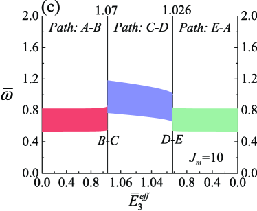
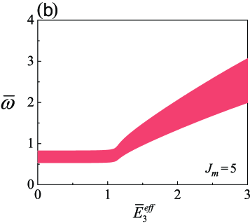
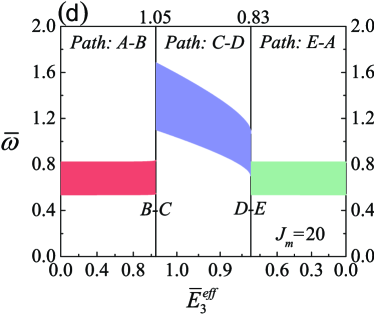
Figure 4: The frequency limits of the first band gap of incremental shear waves versus the dimensionless electric field $\overline{E}_{3}^{\text{eff}}$ in the periodic DE laminate for the N-H model (a) and the Gent model with (b) ${{J}_{m}}=5$, (c) ${{J}_{m}}=10$ and (d) ${{J}_{m}}=20$.

Based on the nonlinear response of different strain-stiffening models with or without the snap-through transition, it is extremely feasible to electrostatically tune the band structures of incremental waves in DE laminates in various manners. For the Gent model with $J_{m}=10$ and different electric fields, the dispersion curves of incremental shear waves are depicted in Figs. 3(a) and 3(b) before and after the snap-through transition, respectively. It is observed that the band gaps appear at the center and border of the first Brillouin zone and their positions move up with increasing electric field. Comparing the result in Fig. 3(a) with that in Fig. 3(b), we can see that a huge change in dispersion curves can be achieved by means of the snap-through transition.

To clearly demonstrate the effect of snap-through instabilities on the band gaps, the first band gap of incremental shear waves is taken as an example and its variations with the normalized effective electric field are displayed in Fig. 4(a)-(d) for the ideal N-H and Gent models (${{J}_{m}}=5$, 10 and 20). Hereafter, all the critical electric field value $\overline{E}_{3}^{\text{cr}}$ will be marked out on the top of corresponding figures. We observe from Fig. 4(a) that the first band gap of shear waves in ideal N-H DE laminates is not affected by the variation of electric stimuli, which agrees well with the result of Galich et al. (2017) for the compressible periodic hyperelastic laminate. This phenomenon can be ascribed to the mutual cancellation between the change in geometrical and material properties via the finite deformation induced by electric stimuli. For the ideal Gent models with $J_{m}=20$ and 10 shown in Figs. 4(c) and 4(d), we can obtain that the snap-through transition triggered at the corresponding critical electric field leads to a remarkable change in the position and width of shear wave band gap, and the subsequent decrease in the electric field from state $C$ to state $D$ lowers the position and narrows the width of band gap continuously. Besides, the results along the loading path $E$-$A$ coincide with those along path $A$-$B$ and their variation trend of the first band gaps of shear waves for ${{J}_{m}}=10$ and 20 appears to be the same as that of the N-H model, which can be explained based on the fact that the Gent phase has not reached the strain-stiffening stage under a small electric field and resembles the N-H model. Different from Figs. 4(c) and 4(d), Fig. 4(b) presents the continuous band gap variation with increasing electric field $\overline{E}_{3}^{\text{eff}}$ for the ideal Gent model ${{J}_{m}}=5$ without the snap-through instability. To be specific, the band gap widens and lifts up beyond a threshold value of the effective electric field ($\overline{E}_{3}^{\text{eff}}\simeq 1.15$), where the influence of strain-stiffening effect (belonging to the material property change) exceeds that of geometrical change on the shear wave band gap.

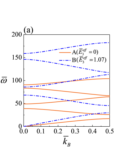
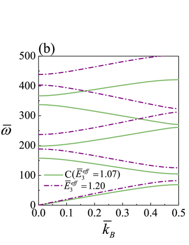
Figure 5: Evolution of the band structures of longitudinal waves before (a) and after (b) the snap-through transition from states $B$ to $C$ shown in Fig. 2 (${{J}_{m}}=10$).

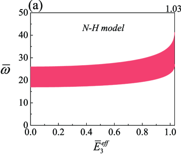
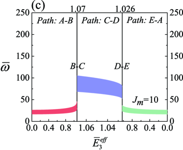
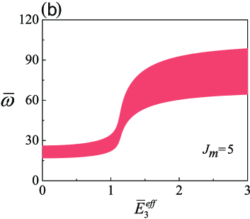
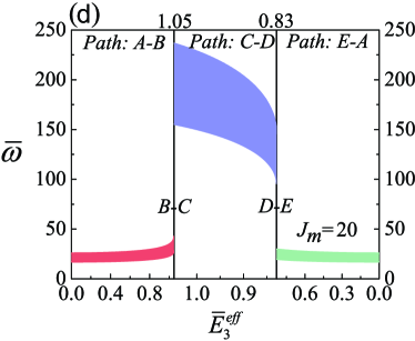
Figure 6: The frequency limits of the first band gap of incremental longitudinal waves versus the dimensionless electric field $\overline{E}_{3}^{\text{eff}}$ in the periodic DE laminate for the N-H model (a) and the Gent model with (b) ${{J}_{m}}=5$, (c) ${{J}_{m}}=10$ and (d) ${{J}_{m}}=20$.

Similarly, for the ideal Gent model with $J_{m}=10$ and different electric stimuli, Figs. 5(a) and 5(b) show the evolution of dispersion diagrams of incremental longitudinal (or pressure) waves propagating in the periodic DE laminate before and after snap-through transition, respectively. Analogous observations to those in Figs. 3(a) and 3(b) can be obtained and hence the discussions are omitted for brevity. Nevertheless, it should be emphasized that the position or the frequency of band gaps for pressure waves is much higher than that for shear waves when comparing Figs. 5(a) and 5(b) with Figs. 3(a) and 3(b).

Furthermore, for incremental pressure waves, Figs. 6(a)-(d) display the frequency limits of the first band gap as functions of the normalized electric field for the ideal N-H model and the Gent models with ${{J}_{m}}=5$, 10 and 20. We find from Figs. 6(a)-(c) that the pressure wave band gap for the N-H model before the snap-through transition can be altered by the electric stimuli, which is distinguished from the case of shear waves, since the dominant mechanism affecting the pressure wave band gaps is the geometrical change of layers via the finite deformation generated by the electric field (Galich et al., 2017). Specifically, the pressure wave band gap moves upward owing to the geometrical change as the electric field increases although the material may not reach the strain-stiffening stage before the snap-through transition. Comparing the variation trends at the snap-through transitions and at the loading path $C$-$D$ for pressure waves in Figs. 6(c) and 6(d) with those for shear waves in Figs. 4(c) and 4(d), we can obtain qualitatively similar characteristics and will not repeat here. However, we note that compared with the result of tuning incremental shear waves, a better tunable effect on pressure waves can be obtained in view of a relatively greater jump in the band gap induced by the snap-through transition. In addition, for the ideal Gent model with $J_{m}=5$ shown in Fig. 6(b), we see that before the same threshold value $\overline{E}_{3}^{\text{eff}}\simeq 1.15$ as that in Fig. 4(b), the first band gap of longitudinal waves ascends and keeps the same width with the increase of electric field. A further increase in electric field makes the band gap move upward and become wider due to the combination effects of strain stiffening and great geometrical change in the compressible ideal DE laminate. Finally, the band gap may reach a plateau at the lock-up stretch $\lambda_{lim}$, where the layers of DE laminate have been compressed sufficiently such that the strain stiffening and the geometrical configuration almost keep unchanged.

In a word, by choosing DE materials with different Gent constants ${{J}_{m}}$ reflecting the strength of strain-stiffening effect, sharp transition and continuous control of band gaps are practicable by tuning the electric field for both shear and longitudinal waves, which should be beneficial for the design of tunable acoustic/elastic wave devices.

5.2 Influence of the second strain invariant

Now the effect of the second strain invariant $I_{2}$ characterized by the second modulus $c_{2}$ on the nonlinear response and wave propagation behavior in periodic DE laminates is considered in this subsection without electrostrictive effect and prestress ($\tau_{33}^{0}=\gamma_{0}=\gamma_{2}=0$ and $\gamma_{1}=1$). By virtue of fitting experimental data with the Gent-Gent constitutive model for the mechanical response of natural rubbers, Ogden et al. (2004) obtained two sets of parameters with ${c_{2}}/\mu=$ 0.42 and 0.14 for simple tension and equibiaxial tension, respectively. Recently, Chen et al. (2019a) performed the pure-shear tests on three different DE materials: the THERABAND YELLOW 11726 made of styrenic rubber, the OPPO BAND GREEN 8003 made of natural rubber and VHB 4905 by 3M, with ${c_{2}}/\mu$ measured as 0.91, 0.37 and 0.00024, respectively. In our work, the normalized material parameter $\bar{c}_{2}$ used for numerical calculations is chosen as 0, 0.37 and 0.91 in accordance with the experimental results obtained by Chen et al. (2019a).

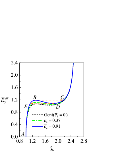
Figure 7: Nonlinear response of the lateral stretch $\lambda$ to the normalized effective referential electric field $\overline{E}_{3}^{\text{eff}}$ in the DE laminate for Gent-Gent model with ${\bar{c}_{2}}=$ 0 (original Gent model), 0.37 and 0.91 ($J_{m}=$10).

Fig. 7 displays the nonlinear response of the periodic ideal DE laminate under electric stimuli for the compressible Gent-Gent model (18) with different values of ${\bar{c}_{2}}=$ 0, 0.37 and 0.91 ($J_{m}=$ 10, $\tau_{33}^{0}=\gamma_{0}=\gamma_{2}=0$ and $\gamma_{1}=1$). We observe that the increase in ${\bar{c}_{2}}$ may result in larger critical electric field at which the snap-through instability from state $B$ to state $C$ takes place and the resulting lateral stretch at the stable state $C$ also becomes larger. However, the nonlinear responses at small and large effective electric fields ($\overline{E}_{3}^{\text{eff}}\lesssim 1.0$ and $\overline{E}_{3}^{\text{eff}}\gtrsim 1.2$) appear to be independent of the second strain invariant.

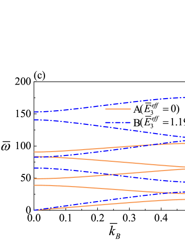
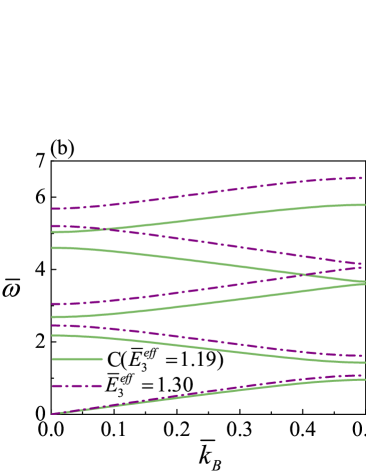
Figure 8: Evolution of the band structures of shear (a, b) and longitudinal (c, d) waves before (a, c) and after (b, d) the snap-through transition from states $B$ to $C$ shown in Fig. 7 for ${\bar{c}_{2}}=$ 0.91 (${{J}_{m}}=10$).

The evolution of band structures for incremental shear and longitudinal waves before and after the snap-through transition is displayed in Fig. 8 for ${\bar{c}_{2}}=0.91$ and different electric fields. We find from Fig. 8 that the band gaps can be moved up by increasing the electric field, and the triggered snap-through transition helps to realize a drastic change in band gaps. In addition, by comparing the results in Figs. 8(c) and (d) with those in Figs. 8(a) and (b), we see that the band gap frequency of longitudinal waves is much larger than that of shear waves. These are qualitatively analogous to the phenomena observed in Figs. 3 and 5.

In order to clearly show the effect of the second strain invariant on wave propagation behaviors, Fig. 9 depicts the frequency limits of the first shear and pressure wave band gaps versus the effective electric field before (path $A$ to $B$) and after (path $C$ to $D$) the snap-through transtion at three different values of ${\bar{c}_{2}}=$ 0, 0.37 and 0.91. The result for ${\bar{c}_{2}}=$ 0 corresponds to the case of the original Gent model. For different ${\bar{c}_{2}}$, the variation trends of frequency limits with electric field $\overline{E}_{3}^{\text{eff}}$ are qualitatively consistent but quantitatively different for both loading paths. The differences are as follows: (1) the critical electric field becomes larger and the frequency limits (i.e. the position of band gaps) are lifted up with the increase of ${\bar{c}_{2}}$; (2) the band gaps of both shear and pressure waves can be tuned in a wider range of electric field for a larger ${\bar{c}_{2}}$.

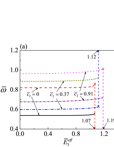
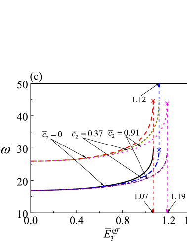
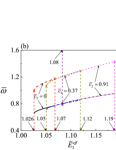
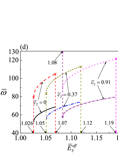
Figure 9: The frequency limits of the first shear (a, b) and longitudinal (c, d) wave band gap versus the dimensionless electric field $\overline{E}_{3}^{\text{eff}}$ in the ideal DE laminate before (a, c) and after (b, d) the snap-through transition for ${{J}_{m}}=10$ and different ${\bar{c}_{2}}$ (The corresponding critical $\overline{E}_{3}^{\text{cr}}$ is also marked by cross in this figure).

5.3 Influence of the electrostrictive effect

Reference	${{\gamma}_{\text{0}}}$	${{\gamma}_{\text{1}}}$	${{\gamma}_{\text{2}}}$
ES-1 (Wissler and Mazza, 2007)	0.00104	1.14904	-0.15008
ES-2 (Li et al., 2011)	0.00458	1.3298	-0.33438

Table 1: Electrostrictive parameters of the enriched Gent DE model utilized in numerical calculations (‘ES-1’ denotes the first set of electrostrictive parameters from Wissler and Mazza (2007), while ‘ES-2’ represents the second one from Li et al. (2011)).

Due to the large deformations of DEs induced by the application of electric fields, the dielectric permittivity is no longer a constant and dependent on the deformation process, which is referred to as the electrostrictive effect (Zhao and Suo, 2008). This phenomenon has been observed by the experimental works (Wissler and Mazza, 2007; Li et al., 2011) for typical DE materials (such as 3M VHB4910). By means of the numerical fitting of the enriched material model (16) to experimental data, Gei et al. (2014) obtained the values of electrostrictive parameters for experimentally tested DE materials conducted by Wissler and Mazza (2007) and Li et al. (2011). The two sets of electrostrictive parameters marked by ‘ES-1’ and ‘ES-2’ are provided in Table 1. In this subsection, we will illustrate the effect of electrostriction on nonlinear response and incremental wave characteristics of the periodic DE laminate under electric stimuli. Note that A provides some other electrostrictive models available in the literature (Zhao and Suo, 2008; Dorfmann and Ogden, 2010; Vertechy et al., 2013), numerical comparison of which is beyond the scope of this paper and worth further research.

Based on Eqs. (21) and (23), the nonlinear response of the periodic DE laminate to the electric stimuli are displayed in Fig. 10 for the ideal ($\gamma_{0}=\gamma_{2}=0$ and $\gamma_{1}=1$) and enriched Gent models with the electrostrictive effect. Note that the prestress here is still set to be $\tau_{33}^{0}=0$ and the Gent constant is taken as ${{J}_{m}}=10$ for all three cases. For small effective electric fields ($\overline{E}_{3}^{\text{eff}}\lesssim 0.8$) where the effect of electrostriction can be neglected, the results predicted by the electrostrictive model are the same as that based on the ideal Gent model. When considering the electrostriction effect, the critical electric field $\overline{E}_{3}^{\text{cr}}$ of the enriched Gent model where the snap-through transition from state $B$ to state $C$ occurs is higher than that given by the ideal Gent model. However, the critical stretch $\lambda_{\text{cr}}$ at state $B$ is almost independent of the electrostrictive parameters. Moreover, the enriched Gent DE laminate may achieve a smaller lateral stretch $\lambda$ at the stable state $C$ after snap-through transition.

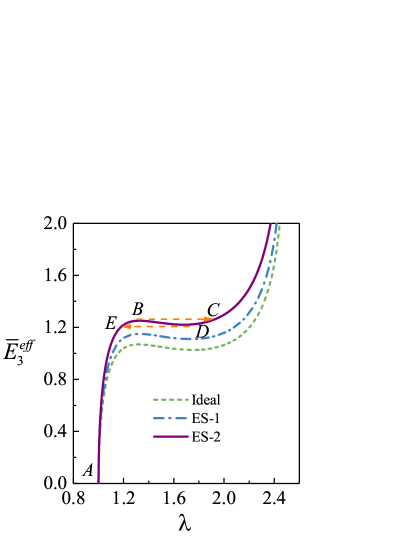
Figure 10: Nonlinear response of the periodic DE laminate to the effective electric field for the ideal, ES-1 and ES-2 Gent models (${{J}_{m}}=10$).

For the first band gap of incremental shear waves, we highlight in Figs. 11(a) and 11(b) the dependence of prohibited frequency limits on the dimensionless effective electric field for ES-1 and ES-2 enriched Gent model ($J_{m}=10$), respectively. We see from Fig. 11(a) that the variation trend for ES-1 parameters is qualitatively analogous to that in Fig. 4(c) for the ideal model except for the various critical electric field values $\overline{E}_{3}^{\text{cr}}$. Nonetheless, the shear wave band gap of the enriched Gent DE laminate with ES-2 parameters shown in Fig. 11(b) exhibits different variation features when subjected to the electric field. Specifically, when the applied electric field increases from zero to the critical value $\overline{E}_{3}^{\text{cr}}$ (from $A$ to $B$), the frequency limits first decrease and then increase slightly. Additionally, when adopting ES-2 parameters (Li et al., 2011), the jump of band gap during the snap-through transition from $B$ to $C$ is not so significant as those in Figs. 4(c) and 11(a).

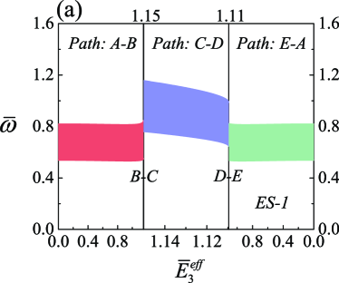
Figure 11: The frequency limits of the first band gap of incremental shear waves versus the dimensionless electric field $\overline{E}_{3}^{\text{eff}}$ in the periodic DE laminate for the enriched Gent model ($J_{m}=10$) with different electrostriction parameters: (a) ES-1; (b) ES-2.

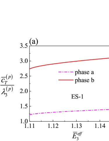
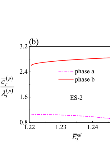
Figure 12: The variation of parameter $\bar{c}_{T}^{\left(p\right)}/\lambda_{3}^{\left(p\right)}$ for both DE phases with the dimensionless electric field $\overline{E}_{3}^{\text{eff}}$ for loading path $C$-$D$ and different electrostriction parameters: (a) ES-1; (b) ES-2.

Furthermore, Fig. 11(b) for ES-2 parameters shows that the forbidden frequency of incremental shear waves even increases monotonically with the decrease of $\overline{E}_{3}^{\text{eff}}$ along the path $C$-$D$, in contrast to the monotonous declining in Figs. 4(c) and 11(a). The reason for this phenomenon can be explained as follows. First, we define the effective shear wave velocity as ${c_{T}}=\sqrt{c_{55}^{*}/\rho}$ and hence the wave number is ${k_{T}}=\omega/{c_{T}}$. Then, the terms ${k_{T}}h$ in Eq. (36) for each phase can be rewritten as $\bar{\omega}{\lambda_{3}}/{\bar{c}_{T}}$, where ${\bar{c}_{T}}=\sqrt{Jc_{55}^{*}/{\mu_{0}}}$. It is well-known that the frequency of band gaps depends on the dimensionless wave velocity ${\bar{c}_{T}}$ and stretch ratio ${\lambda_{3}}$ (Galich et al., 2017). Specifically, an increase in ${\bar{c}_{T}}$ stands for the increase of material stiffness, which is accompanied by an ascending change in frequency; conversely, with the increase of ${\lambda_{3}}$, the deformed size of structure becomes larger, which may result in the decrease in frequency. Since ${\bar{c}_{T}}$ and ${\lambda_{3}}$ affect the frequency of band gaps in the opposite way, the variation of parameter ${\bar{c}_{T}}/{\lambda_{3}}$ as a whole with the effective electric field for loading path $C$-$D$ is displayed in Fig. 12 to take the effects of both phase material properties and size into consideration. As we can see from Fig. 12(a) for ES-1, $\bar{c}_{T}^{\left(p\right)}/\lambda_{3}^{\left(p\right)}$ becomes smaller for both phases with the decrease of $\overline{E}_{3}^{\text{eff}}$ from state $C$ to state $D$, which means that the shear wave band gap may be moved downwards by decreasing the electric field, as shown in Fig. 11(a). But for ES-2, Fig. 12(b) demonstrates that the curves of phases $a$ and $b$ vary in opposite trends (i.e., with the decrease of $\overline{E}_{3}^{\text{eff}}$, $\bar{c}_{T}^{\left(p\right)}/\lambda_{3}^{\left(p\right)}$ increases for phase $a$, but decreases for phase $b$). Because the increase in $\bar{c}_{T}^{\left(a\right)}/\lambda_{3}^{\left(a\right)}$ exceeds the decrease in $\bar{c}_{T}^{\left(b\right)}/\lambda_{3}^{\left(b\right)}$, the shear wave band gap in Fig. 11(b) moves up with the decrease of electric field. Similar explanations can be applied to other loading paths and longitudinal waves.

Fig. 13 illustrates the variation trend of the first band gap of longitudinal waves with the electric field $\overline{E}_{3}^{\text{eff}}$ for the enriched DE model with the ES-1 and ES-2 parameters. Along the loading path $A$-$B$, qualitatively analogous characteristics to those of the ideal Gent DE model are observed, which are different from the results of shear waves. The reason is that the geometrical change dominates the longitudinal wave band gaps and the critical stretch ratio $\lambda_{\text{cr}}$ at state $B$ is almost independent of the effect of electrostriction (as shown in Fig. 10). Besides, both of the two sets of electrostrictive parameters lower the frequency jump for the snap-through transition, compared with the ideal DE model.

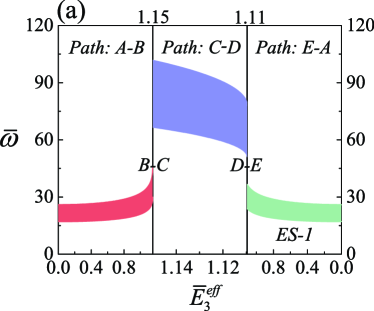
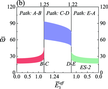
Figure 13: The frequency limits of the first band gap of incremental longitudinal waves versus the dimensionless electric field $\overline{E}_{3}^{\text{eff}}$ in the periodic DE laminate for the enriched Gent model ($J_{m}=10$) with different electrostriction parameters: (a) ES-1; (b) ES-2.

In brief, the electrostrictive effect increases the critical electric field where the snap-through instability happens, and it weakens the sharp transition of band gaps for both shear and longitudinal waves. Since different electrostrictive materials influence the superimposed wave propagation behaviors in different ways (see Fig. 11), a guided wave-based testing method may be developed to characterize the electrostrictive parameters of different DEs.

5.4 Influence of the prestress

Except for the electrostrictive effect discussed in Sec. 5.3, the mechanical loading (here is the prestress ${\tau}_{\text{33}}^{\text{0}}$ in the thickness direction displayed in Fig. 1) can also be exploited to tune the snap-through instabilities and manipulate the wave propagation in the periodic DE laminate. For the ideal Gent model with $J_{m}=10$, the nonlinear response of the periodic DE laminate under electric stimuli are plotted in Fig. 14 for different prestress values of $\overline{\tau}_{\text{33}}^{\text{0}}=0,1,2$ and 4. We see from Fig. 14 that a larger prestress is accompanied by a smaller lateral stretch $\lambda$ at the initial state $A$ ($\overline{E}_{3}^{\text{eff}}=0$). The critical electric fields $\overline{E}_{3}^{\text{cr}}$ at states $B$ and $D$ rises with the increase of prestress, which implies that the application of prestress in the thickness direction is beneficial to stabilizing the periodic DE laminate. Moreover, as the prestress increases, the resulting lateral deformation at stable state $C$ after the snap-through transition triggered by electric field becomes remarkably larger. Finally, independent of the applied prestress, the nonlinear responses approach to a vertical asymptote, where the Gent DE laminate reaches the lock-up stretch state that can be calculated as $\lambda_{lim}\simeq 2.55$ according to $J_{m}=2{\lambda_{lim}^{2}}+{\lambda_{lim}^{-4}}-3=10$.

Figure 14: Nonlinear response of the lateral stretch $\lambda$ to the effective electric field $\overline{E}_{3}^{\text{eff}}$ in the periodic DE laminate subjected to different prestress values of $\overline{\tau}_{\text{33}}^{\text{0}}=0,1,2,4$ (the ideal Gent model with ${{J}_{m}}=10$ is adopted).

For different prestress values, the first band gaps of shear and longitudinal waves as functions of the dimensionless electric field are demonstrated in Figs. 15 and 16, respectively, for the ideal Gent DE laminate with $J_{m}=10$. We can obtain qualitatively the same variation trends as those in Figs. 4(c) and 6(c) for zero prestress state: as the electric field ascends to the critical value, the shear wave band gap in path $A$-$B$ may hardly be changed, while the longitudinal one increases monotonically; along path $C$-$D$, the band gaps for both shear and longitudinal waves are shifted to lower frequencies with their width becoming narrower. Nevertheless, it should be emphasized that the jump of band gaps from state $B$ to state $C$ via the snap-through transition becomes more significant with increasing prestress for both types of waves. What’s more, the band gaps in path $C$-$D$ can be continuously adjusted in a wider range of the electric field. We can take the shear waves in Fig. 15 as the example: for $\overline{\tau}_{33}^{0}=1$, the applied electric field can be tuned from 1.20 to 1.06 (i.e., from state $C$ to state $D$ in Fig. 14) with its central frequency varying from 1.17 to 1.02 , while for $\overline{\tau}_{33}^{0}=4$, the electric field changes from 1.74 to 1.14 with the tuning range of central frequency from 1.81 to 0.91.

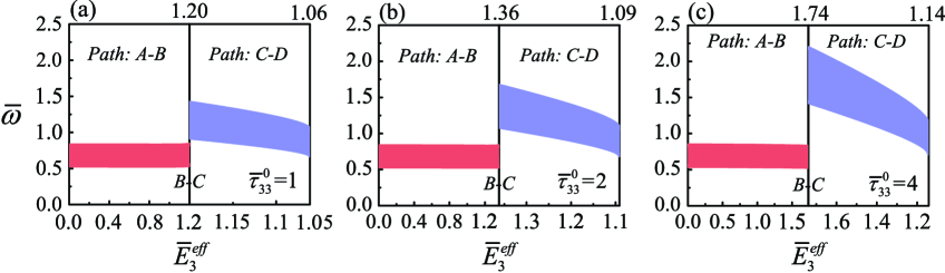
Figure 15: The frequency limits of the first band gap of incremental shear waves versus the dimensionless electric field $\overline{E}_{3}^{\text{eff}}$ in the periodic DE laminate for the ideal Gent model ($J_{m}=10$) and various prestress values: (a) $\overline{\tau}_{33}^{0}=1$; (b) $\overline{\tau}_{33}^{0}=2$; (c) $\overline{\tau}_{33}^{0}=4$.

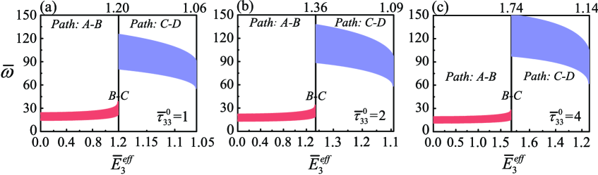
Figure 16: The frequency limits of the first band gap of incremental longitudinal waves versus the dimensionless electric field $\overline{E}_{3}^{\text{eff}}$ in the periodic DE laminate for the ideal Gent model ($J_{m}=10$) and various prestress values: (a) $\overline{\tau}_{33}^{0}=1$; (b) $\overline{\tau}_{33}^{0}=2$; (c) $\overline{\tau}_{33}^{0}=4$.

6 Conclusions

The nonlinear response and superimposed elastic wave motions in an infinite periodic DE laminate subjected to electromechanical loadings are theoretically investigated in this work. First of all, the theory of nonlinear electroelasticity proposed by Dorfmann and Ogden is employed to describe the nonlinear static deformations in periodic DE laminates under combined action of prestress and electric field, where the enriched Gent-Gent DE model is used to characterize the strain-stiffening, the second strain invariant and electrostrictive effects. Utilizing the transfer matrix method as well as the Bloch-Floquet theorem, the dispersion relations of decoupled shear and longitudinal waves superimposed on finite deformations are obtained, which are in the same form as the purely elastic counterpart. At last, numerical investigations are conducted to demonstrate how the material properties and external stimuli affect the nonlinear static response and wave propagation characteristic. What follows is a list of useful numerical findings from the present investigation:

1. For the periodic DE laminate described by ideal Gent model, the snap-through instability originating from geometrical and material nonlinearities can be harnessed to achieve the drastic change in geometrical configuration and band gaps (including the position and width).

2. The snap-through transition may not appear when the strain-stiffening effect is strong enough (such as ${{J}_{m}}=5$) or when the neo-Hookean model is adopted. Thus, the shear and pressure wave band gaps can be tuned continuously by adjusting the electric field.

3. Increasing the second modulus raises the critical electric field and lifts up the position of band gaps for both types of waves;

4. Both the electrostrictive effect and applied prestress contribute to stabilizing the periodic DE laminate. However, they affect the band structure in different manners: the former weakens the band gap jump induced by the snap-through transition, while the latter strengthens the tunable frequency range for both types of waves.

5. Due to the difference in physical mechanism dominating the wave motions, the electrostatically tunable effect on the band gap of longitudinal waves is more evident than that on the shear wave band gap.

The results obtained here may provide a strong theoretical guidance for the design and fabrication of electrostatically tunable DE wave devices and for the wave-based characterization method of electrostrictive materials. Experiments will definitely be beneficial to understand the wave propagation behaviors in periodic DE laminates, but they are out of the scope of this paper.

Note that viscoelasticity neglected in this work is indeed an important factor in the analysis of wave propagation behaviors. However, it should be emphasized that the dissipation/damping effect of soft materials on wave propagation is generally significant in the high frequency range, but is usually negligible at low frequencies (see, for example, Li et al. (2017a, 2018, 2019) and Gao et al. (2019)). Here we mainly focus on the first-order band gap in periodic DE laminates, which is the most important one in real-life situations. Numerical calculations indicate that the frequency of the first-order shear wave band gap is relatively low, but that of the pressure wave band gap is a little higher. As a result, the dissipation/damping in DE materials will hardly affect the first-order shear wave band gap while it will have remarkable suppressive effect on the first-order pressure wave band gap. Thus, consideration of dissipation can potentially improve the predictions of the first-order pressure wave band gap, which demands further research.

Appendix A Representative electrostrictive models

This appendix will list the specific forms of energy density function for several representative electrostrictive models suggested in the literature to characterize isotropic DE materials. The energy density function $\Omega^{\text{elec}}({\bf{F}},\bm{\mathcal{D}})$ related to the electrostrictive effect and purely electrostatic field is usually assumed to linearly depend on the three invariants ${I_{4}}$, ${I_{5}}$ and ${I_{6}}$ as

$$\Omega^{\text{elec}}({\bf{F}},\bm{\mathcal{D}})=\frac{1}{{2{\varepsilon}J}}(\gamma_{0}{I_{4}}+\gamma_{1}{I_{5}}+\gamma_{2}{I_{6}}),$$ (41)

where ${{\varepsilon}}={{\varepsilon}_{0}}\varepsilon_{r}$ is the material permittivity in the undeformed state. In general, the three coefficients $\gamma_{0}$, $\gamma_{1}$ and $\gamma_{2}$ are functions of the other three invariants ${I_{1}}$, ${I_{2}}$ and ${I_{3}}$ associated with the deformation. For constant coefficients, Eq. (41) recovers the compressible enriched DE model (16) (Galich and Rudykh, 2016) and the incompressible electrostrictive model with $J=1$ (Gei et al., 2014). Furthermore, if $\gamma_{2}=0$ and $J=1$, Eq. (41) reduces to the incompressible electrostrictive model used in Dorfmann and Ogden (2010).

Moreover, neglecting the dependence on ${I_{4}}$ and ${I_{6}}$, Eq. (41) becomes

$$\Omega^{\text{elec}}({\bf{F}},\bm{\mathcal{D}})=\frac{\gamma_{1}({\bf{F}})}{{2{\varepsilon}J}}{I_{5}}\equiv\frac{{I_{5}}}{{2J{\varepsilon_{d}}({\bf{F}})}},$$ (42)

where ${\varepsilon_{d}}({\bf{F}})={\varepsilon}/{\gamma_{1}({\bf{F}})}$ is the deformation-dependent material permittivity. The soft electro-active material characterized by Eq. (42) is called quasilinear dielectrics (Zhao and Suo, 2008).

Based on the free energy density function $\Psi({\mathbf{F}},\mathbf{E})$ per unit mass rather than the total energy density function $\Omega(\mathbf{F},\bm{\mathcal{D}})$ and using Eulerian electric field vector $\mathbf{E}$ as independent electric variable instead of Lagrangian electric displacement vector $\bm{\mathcal{D}}$ adopted in this work, Vertechy et al. (2013) obtained the nonlinear constitutive equations (neglecting terms related to temperature field in their work) as

$${\bm{\tau}}=\rho\frac{\partial\Psi}{\partial\mathbf{F}}{{\mathbf{F}}^{\text{T}}}+{{\bm{\sigma}}_{\text{M}}}+\mathbf{E}\otimes\mathbf{P},\quad\mathbf{P}=-\rho\frac{\partial\Psi}{\partial\mathbf{E}},$$ (43)

where ${{\bm{\sigma}}_{\text{M}}}={{\varepsilon}_{0}}[\mathbf{E}\otimes\mathbf{E}-(\mathbf{E}\cdot\mathbf{E})\mathbf{I}/2]$ is the well-known Maxwell’s stress tensor in vacuum and $\mathbf{P}=\mathbf{D}-{{\varepsilon}_{0}}\mathbf{E}$ is the electric polarization vector. It has been verified (see Secs. 2.4 and 2.5 in the review work by Wu et al. (2016)) that the nonlinear constitutive equation (43) can be transformed to Eq. (5) by introducing the following augmented free energy density function ${{\Omega}^{*}}\left(\mathbf{F},\bm{\mathcal{E}}\right)$ and conducting the following Legendre transformation

$${{\Omega}^{*}}\left(\mathbf{F},\bm{\mathcal{E}}\right)={{\rho}_{0}}\Psi\left(\mathbf{F},\mathbf{E}\right)-\pi\left(\mathbf{F},\mathbf{E}\right),\quad\Omega\left(\mathbf{F},\bm{\mathcal{D}}\right)={{\Omega}^{*}}\left(\mathbf{F},\bm{\mathcal{E}}\right)+\bm{\mathcal{E}}\cdot\bm{\mathcal{D}},$$ (44)

where

$$\pi\left(\mathbf{F},\mathbf{E}\right)={{\varepsilon}_{0}}J\bm{\mathcal{E}}\cdot\left({{\mathbf{C}}^{-1}}\bm{\mathcal{E}}\right)/2={{\varepsilon}_{0}}J\mathbf{E}\cdot\mathbf{E}/2,\quad\bm{\mathcal{E}}\cdot\bm{\mathcal{D}}=J\mathbf{E}\cdot\mathbf{D}.$$ (45)

For isotropic DE materials, $\Psi({\mathbf{F}},\mathbf{E})$ depends on the following six invariants:

$${{\bar{I}}_{1}} =\text{tr}\mathbf{b}=I_{1},\quad{{\bar{I}}_{2}}=\frac{1}{2}\left[{{\left(\text{tr}\mathbf{b}\right)}^{2}}-\text{tr}\left({{\mathbf{b}}^{2}}\right)\right]=I_{2},\quad{{\bar{I}}_{3}}=\det\mathbf{b}={{J}^{2}}=I_{3},$$

$${{\bar{I}}_{4}} =\mathbf{E}\cdot\mathbf{E},\quad{{\bar{I}}_{5}}=\mathbf{E}\cdot\left(\mathbf{bE}\right),\quad{{\bar{I}}_{6}}=\mathbf{E}\cdot\left({{\mathbf{b}}^{2}}\mathbf{E}\right),$$ (46)

substitution of which into Eq. (43) yields

$${\bm{\tau}}=2\rho\left[\left({{\Psi}_{1}}+{{\Psi}_{2}}{{{\bar{I}}}_{1}}\right)\mathbf{b}-{{\Psi}_{2}}{{\mathbf{b}}^{2}}+{{\Psi}_{3}}{{{\bar{I}}}_{3}}\mathbf{1}-{{\Psi}_{4}}\mathbf{E}\otimes\mathbf{E}+{{\Psi}_{6}}\left(\mathbf{bE}\right)\otimes\left(\mathbf{bE}\right)\right]+{{\bm{\sigma}}_{\text{M}}},$$

$$\mathbf{D}=-2\rho\left({{\Psi}_{4}}\mathbf{E}+{{\Psi}_{5}}\mathbf{bE}+{{\Psi}_{6}}{{\mathbf{b}}^{2}}\mathbf{E}\right),$$ (47)

where ${{\Psi}_{i}}=\partial\Psi/\partial{{\bar{I}}_{i}}(i=1-6)$. In particular, Vertechy et al. (2013) proposed a compressible Mooney-Rivlin electrostrictive model with $\Psi({\mathbf{F}},\mathbf{E})$ decomposed in the following three parts

$$\Psi={{\Psi}^{\text{hyel}}}\left({{{\bar{I}}}_{1}},{{{\bar{I}}}_{2}},J\right)+{{\Psi}^{\text{estr}}}\left(J,{{{\bar{I}}}_{4}},{{{\bar{I}}}_{5}}\right)+{{\Psi}^{\text{esta}}}\left(J,{{{\bar{I}}}_{4}}\right),$$

$${{\Psi}^{\text{hyel}}}=\frac{1}{{{\rho}_{0}}}\left[{{c}_{10}}\left({{{\bar{I}}}_{1}}-3\right)+{{c}_{20}}\left({{{\bar{I}}}_{2}}-3\right)+{{c}_{30}}{{\left(J-1\right)}^{2}}-2\left({{c}_{10}}+2{{c}_{20}}\right)\ln J\right],$$

$${{\Psi}^{\text{estr}}}=-\frac{1}{2{{\rho}_{0}}}\left[\frac{{{\beta}_{10}}\left({{{\bar{I}}}_{5}}-{{{\bar{I}}}_{4}}\right)J}{2}+{{\beta}_{20}}{{{\bar{I}}}_{5}}\left(J-1\right)\right],\quad{{\Psi}^{\text{esta}}}=-{{\varepsilon}_{0}}\frac{{{\chi}_{0}}{{{\bar{I}}}_{4}}J}{2{{\rho}_{0}}},$$ (48)

where $c_{10}$, $c_{20}$, $c_{30}$, $\beta_{10}$ and $\beta_{20}$ are constant material parameters and ${{\chi}_{0}}={{\varepsilon}_{r}}-1$ is the electric susceptibility. The detailed explanation of the three parts in Eq. (A) can be found in Vertechy et al. (2013). Inserting Eq. (A) into Eq. (A) leads to specific constitutive relations (see Eqs. (80)-(81) and (85)-(87) in Vertechy et al. (2013)). Note that due to the different choices of energy density function and independent electric variable, it is intractable to establish a direct and explicit connection between the nonlinear constitutive equations (3) and those in Vertechy et al. (2013).

Appendix B Nonzero components of instantaneous elelctroelastic moduli used in this paper

According to the formulations derived by Dorfmann and Ogden (2010) and Galich and Rudykh (2016) and for the compressible Gent-Gent DE model in Eqs. (16) and (18), the nonzero components of instantaneous elelctroelastic moduli tensors ${{\bm{\mathcal{A}}}_{0}}$, ${{\bm{\mathcal{M}}}_{0}}$ and ${{\bm{\mathcal{R}}}_{0}}$ utilized in Sec. 4 read

$${\cal A}_{03131} ={\cal A}_{03232}=\frac{{{\mu}}}{{{J}}}\frac{{J_{m}}}{{J_{m}-I_{1}+3}}{\lambda_{3}^{2}}+{\color[rgb]{1,0,0}\frac{{2{\lambda_{3}}{c_{2}}}}{{{I_{2}}}}}+\frac{{D_{3}^{2}}}{{{\varepsilon}}}\left[{\gamma_{1}+\left({{\lambda^{2}}+2{\lambda_{3}^{2}}}\right)\gamma_{2}}\right],$$

$${\cal A}_{03333} ={\lambda^{2}}\lambda_{3}\left({\Lambda_{0}-\frac{{2{\mu}}}{{J_{m}}}}\right)+\frac{{{\mu}}}{{{\lambda^{2}}\lambda_{3}}}\left[{\frac{{J_{m}}}{{J_{m}-I_{1}+3}}{\lambda_{3}^{2}}+1}\right]+{\color[rgb]{1,0,0}\frac{{4{\lambda_{3}}{c_{2}}}}{{{I_{2}}}}\left({1-\frac{{4{\lambda^{2}}\lambda_{3}^{2}}}{{{I_{2}}}}}\right)}$$

$$+\frac{{2{\mu}}}{{{\lambda^{2}}\lambda_{3}}}\frac{{J_{m}}}{{{{\left({J_{m}-I_{1}+3}\right)}^{2}}}}{\lambda_{3}^{4}}+\frac{{D_{3}^{2}}}{{{\varepsilon}}}\left({{\lambda_{3}^{-2}}\gamma_{0}+3{\lambda_{3}^{2}}\gamma_{2}}\right),$$

$${\cal M}_{0311} ={\cal M}_{0322}=\frac{{{D_{3}}}}{{{\varepsilon}}}\left[{\gamma_{1}+\left({{\lambda^{2}}+{\lambda_{3}^{2}}}\right)\gamma_{2}}\right],$$

$${\cal R}_{011} =\frac{1}{{{\varepsilon}}}\left({{\lambda^{-2}}\gamma_{0}+\gamma_{1}+{\lambda^{2}}\gamma_{2}}\right).$$

References

References

- Adler (1990) Adler, E. L., 1990. Matrix methods applied to acoustic waves in multilayers. IEEE Transactions on Ultrasonics, Ferroelectrics, and Frequency Control 37 (6), 485–490.
- Bertoldi et al. (2017) Bertoldi, K., Vitelli, V., Christensen, J., van Hecke, M., 2017. Flexible mechanical metamaterials. Nature Reviews Materials 2 (11), 17066.
- Bortot et al. (2018) Bortot, E., Amir, O., Shmuel, G., 2018. Topology optimization of dielectric elastomers for wide tunable band gaps. International Journal of Solids and Structures 143, 262–273.
- Bortot and Shmuel (2017) Bortot, E., Shmuel, G., 2017. Tuning sound with soft dielectrics. Smart Materials and Structures 26 (4), 045028.
- Chen and Dai (2012) Chen, W., Dai, H., 2012. Waves in pre-stretched incompressible soft electroactive cylinders: Exact solution. Acta Mechanica Solida Sinica 25 (5), 530–541.
- Chen et al. (2019a) Chen, Y., Agostini, L., Moretti, G., Fontana, M., Vertechy, R., 2019a. Dielectric elastomer materials for large-strain actuation and energy harvesting: A comparison between styrenic rubber, natural rubber and acrylic elastomer. Smart Materials and Structures 28 (11), 114001.
- Chen et al. (2019b) Chen, Y. J., Wu, B., Su, Y. P., Chen, W. Q., 2019b. Tunable two-way unidirectional acoustic diodes: Design and simulation. Journal of Applied Mechanics 86 (3), 031010.
- Dorfmann and Ogden (2005) Dorfmann, L., Ogden, R. W., 2005. Nonlinear electroelasticity. Acta Mechanica 174 (3-4), 167–183.
- Dorfmann and Ogden (2006) Dorfmann, L., Ogden, R. W., 2006. Nonlinear electroelastic deformations. Journal of Elasticity 82 (2), 99–127.
- Dorfmann and Ogden (2010) Dorfmann, L., Ogden, R. W., 2010. Electroelastic waves in a finitely deformed electroactive material. IMA Journal of Applied Mathematics 75 (4), 603–636.
- Dorfmann and Ogden (2014) Dorfmann, L., Ogden, R. W., 2014. Nonlinear Theory of Electroelastic and Magnetoelastic Interactions. Springer, New York.
- Galich et al. (2017) Galich, P. I., Fang, N. X., Boyce, M. C., Rudykh, S., 2017. Elastic wave propagation in finitely deformed layered materials. Journal of the Mechanics and Physics of Solids 98, 390–410.
- Galich and Rudykh (2016) Galich, P. I., Rudykh, S., 2016. Manipulating pressure and shear waves in dielectric elastomers via external electric stimuli. International Journal of Solids and Structures 91, 18–25.
- Galich and Rudykh (2017) Galich, P. I., Rudykh, S., 2017. Shear wave propagation and band gaps in finitely deformed dielectric elastomer laminates: Long wave estimates and exact solution. Journal of Applied Mechanics 84 (9), 091002.
- Gao et al. (2017) Gao, N., Hou, H., Mu, Y., 2017. Low frequency acoustic properties of bilayer membrane acoustic metamaterial with magnetic oscillator. Theoretical and Applied Mechanics Letters 7 (4), 252–257.
- Gao et al. (2018) Gao, N., Huang, Y. L., Bao, R. H., Chen, W. Q., 2018. Robustly tuning bandgaps in two-dimensional soft phononic crystals with criss-crossed elliptical holes. Acta Mechanica Solida Sinica 31 (5), 573–588.
- Gao et al. (2019) Gao, N., Li, J., Bao, R. H., Chen, W. Q., 2019. Harnessing uniaxial tension to tune poisson’s ratio and wave propagation in soft porous phononic crystals: An experimental study. Soft Matter 15 (14), 2921–2927.
- Gei et al. (2014) Gei, M., Colonnelli, S., Springhetti, R., 2014. The role of electrostriction on the stability of dielectric elastomer actuators. International Journal of Solids and Structures 51 (3-4), 848–860.
- Gei et al. (2010) Gei, M., Roccabianca, S., Bacca, M., 2010. Controlling bandgap in electroactive polymer-based structures. IEEE/ASME Transactions on Mechatronics 16 (1), 102–107.
- Gent (1996) Gent, A., 1996. A new constitutive relation for rubber. Rubber Chemistry and Technology 69 (1), 59–61.
- Getz and Shmuel (2017) Getz, R., Shmuel, G., 2017. Band gap tunability in deformable dielectric composite plates. International Journal of Solids and Structures 128, 11–22.
- Holzapfel (2000) Holzapfel, G. A., 2000. Nonlinear Solid Mechanics: A Continuum Approach for Engineering. John Wiley & Sons, Chichester.
- Huang et al. (2013) Huang, J., Shian, S., Suo, Z., Clarke, D. R., 2013. Maximizing the energy density of dielectric elastomer generators using equi-biaxial loading. Advanced Functional Materials 23 (40), 5056–5061.
- Huang et al. (2018) Huang, Y. L., Gao, N., Chen, W. Q., Bao, R. H., 2018. Extension/compression-controlled complete band gaps in 2d chiral square-lattice-like structures. Acta Mechanica Solida Sinica 31 (1), 51–65.
- Huang and Wu (2005) Huang, Z., Wu, T., 2005. Temperature effect on the bandgaps of surface and bulk acoustic waves in two-dimensional phononic crystals. IEEE Transactions on Ultrasonics, Ferroelectrics, and Frequency Control 52 (3), 365–370.
- Jandron and Henann (2018) Jandron, M., Henann, D. L., 2018. A numerical simulation capability for electroelastic wave propagation in dielectric elastomer composites: Application to tunable soft phononic crystals. International Journal of Solids and Structures 150, 1–21.
- Kittel (2005) Kittel, C., 2005. Introduction to Solid State Physics. John Wiley & Sons, New York.
- Koh et al. (2010) Koh, S. J. A., Keplinger, C., Li, T., Bauer, S., Suo, Z., 2010. Dielectric elastomer generators: How much energy can be converted? IEEE/ASME Transactions on Mechatronics 16 (1), 33–41.
- Kushwaha et al. (1993) Kushwaha, M. S., Halevi, P., Dobrzynski, L., Djafari-Rouhani, B., 1993. Acoustic band structure of periodic elastic composites. Physical Review Letters 71 (13), 2022.
- Li et al. (2011) Li, B., Chen, H., Qiang, J., Hu, S., Zhu, Z., Wang, Y., 2011. Effect of mechanical pre-stretch on the stabilization of dielectric elastomer actuation. Journal of Physics D: Applied Physics 44 (15), 155301.
- Li and Wang (2012) Li, F. M., Wang, Y. Z., 2012. Elastic wave propagation and localization in band gap materials: A review. Science China Physics, Mechanics and Astronomy 55 (10), 1734–1746.
- Li et al. (2017a) Li, G. Y., He, Q., Mangan, R., Xu, G., Mo, C., Luo, J., Destrade, M., Cao, Y., 2017a. Guided waves in pre-stressed hyperelastic plates and tubes: Application to the ultrasound elastography of thin-walled soft materials. Journal of the Mechanics and Physics of Solids 102, 67–79.
- Li et al. (2019) Li, J., Wang, Y. T., Chen, W. Q., Wang, Y. S., Bao, R. H., 2019. Harnessing inclusions to tune post-buckling deformation and bandgaps of soft porous periodic structures. Journal of Sound and Vibration 459, 114848.
- Li et al. (2018) Li, S., Zhao, D., Niu, H., Zhu, X., Zang, J., 2018. Observation of elastic topological states in soft materials. Nature Communications 9 (1), 1–9.
- Li et al. (2017b) Li, T., Li, G., Liang, Y., Cheng, T., Dai, J., Yang, X., Liu, B., Zeng, Z., Huang, Z., Luo, Y., et al., 2017b. Fast-moving soft electronic fish. Science Advances 3 (4), e1602045.
- Lian et al. (2016) Lian, Z., Jiang, S., Hu, H., Dai, L., Chen, X., Jiang, W., 2016. An enhanced plane wave expansion method to solve piezoelectric phononic crystal with resonant shunting circuits. Shock and Vibration 2016, 4015363.
- Liang et al. (2009) Liang, B., Yuan, B., Cheng, J., 2009. Acoustic diode: Rectification of acoustic energy flux in one-dimensional systems. Physical Review Letters 103 (10), 104301.
- Liu et al. (2015) Liu, L., Zhang, Z., Li, J., Li, T., Liu, Y., Leng, J., 2015. Stability of dielectric elastomer/carbon nanotube composites coupling electrostriction and polarization. Composites Part B: Engineering 78, 35–41.
- Liu et al. (2000) Liu, Z., Zhang, X., Mao, Y., Zhu, Y., Yang, Z., Chan, C. T., Sheng, P., 2000. Locally resonant sonic materials. Science 289 (5485), 1734–1736.
- Lu et al. (2013) Lu, Z., Cui, Y., Zhu, J., Zhao, Z., Debiasi, M., 2013. Acoustic characteristics of a dielectric elastomer absorber. The Journal of the Acoustical Society of America 134 (5), 4218–4218.
- Lu et al. (2015) Lu, Z., Godaba, H., Cui, Y., Foo, C. C., Debiasi, M., Zhu, J., 2015. An electronically tunable duct silencer using dielectric elastomer actuators. The Journal of the Acoustical Society of America 138 (3), EL236–EL241.
- Ma et al. (2018) Ma, F., Huang, M., Xu, Y., Wu, J. H., 2018. Bilayer synergetic coupling double negative acoustic metasurface and cloak. Scientific Reports 8 (1), 5906.
- Mao et al. (2019) Mao, R. W., Wu, B., Carrera, E., Chen, W. Q., 2019. Electrostatically tunable small-amplitude free vibrations of pressurized electro-active spherical balloons. International Journal of Non-Linear Mechanics 117, 103237.
- Matar et al. (2013) Matar, O. B., Vasseur, J. O., Deymier, P. A., 2013. Tunable phononic crystals and metamaterials. In: Acoustic Metamaterials and Phononic Crystals. Springer, Berlin, pp. 253–280.
- Ogden et al. (2004) Ogden, R. W., Saccomandi, G., Sgura, I., 2004. Fitting hyperelastic models to experimental data. Computational Mechanics 34 (6), 484–502.
- Shmuel (2015) Shmuel, G., 2015. Manipulating torsional motions of soft dielectric tubes. Journal of Applied Physics 117 (17), 174902.
- Shmuel and deBotton (2012) Shmuel, G., deBotton, G., 2012. Band-gaps in electrostatically controlled dielectric laminates subjected to incremental shear motions. Journal of the Mechanics and Physics of Solids 60 (11), 1970–1981.
- Shmuel and deBotton (2013) Shmuel, G., deBotton, G., 2013. Axisymmetric wave propagation in finitely deformed dielectric elastomer tubes. Proceedings of the Royal Society A: Mathematical, Physical and Engineering Sciences 469 (2155), 20130071.
- Shmuel and Pernas-Salomón (2016) Shmuel, G., Pernas-Salomón, R., 2016. Manipulating motions of elastomer films by electrostatically-controlled aperiodicity. Smart Materials and Structures 25 (12), 125012.
- Soukiassian et al. (2007) Soukiassian, A., Tian, W., Tenne, D., Xi, X., Schlom, D., Lanzillotti-Kimura, N., Bruchhausen, A., Fainstein, A., Sun, H., Pan, X., et al., 2007. Acoustic bragg mirrors and cavities made using piezoelectric oxides. Applied Physics Letters 90 (4), 042909.
- Su et al. (2016) Su, Y. P., Wang, H. M., Zhang, C. L., Chen, W. Q., 2016. Propagation of non-axisymmetric waves in an infinite soft electroactive hollow cylinder under uniform biasing fields. International Journal of Solids and Structures 81, 262–273.
- Su et al. (2018) Su, Y. P., Wu, B., Chen, W. Q., Lü, C. F., 2018. Optimizing parameters to achieve giant deformation of an incompressible dielectric elastomeric plate. Extreme Mechanics Letters 22, 60–68.
- Sugimoto et al. (2013) Sugimoto, T., Ando, A., Ono, K., Morita, Y., Hosoda, K., Ishii, D., Nakamura, K., 2013. A lightweight push-pull acoustic transducer composed of a pair of dielectric elastomer films. The Journal of the Acoustical Society of America 134 (5), EL432–EL437.
- Vertechy et al. (2013) Vertechy, R., Berselli, G., Parenti Castelli, V., Bergamasco, M., 2013. Continuum thermo-electro-mechanical model for electrostrictive elastomers. Journal of Intelligent Material Systems and Structures 24 (6), 761–778.
- Viry et al. (2014) Viry, L., Levi, A., Totaro, M., Mondini, A., Mattoli, V., Mazzolai, B., Beccai, L., 2014. Flexible three-axial force sensor for soft and highly sensitive artificial touch. Advanced Materials 26 (17), 2659–2664.
- Wang et al. (2013) Wang, P., Shim, J., Bertoldi, K., 2013. Effects of geometric and material nonlinearities on tunable band gaps and low-frequency directionality of phononic crystals. Physical Review B 88 (1), 014304.
- Wang et al. (2020) Wang, Y. F., Wang, Y. Z., Wu, B., Chen, W. Q., Wang, Y. S., 2020. Tunable and active phononic crystals and metamaterials. Applied Mechanics Reviews 72 (4), 040801.
- Wissler and Mazza (2007) Wissler, M., Mazza, E., 2007. Electromechanical coupling in dielectric elastomer actuators. Sensors and Actuators A: Physical 138 (2), 384–393.
- Wu et al. (2017) Wu, B., Su, Y. P., Chen, W. Q., Zhang, C. Z., 2017. On guided circumferential waves in soft electroactive tubes under radially inhomogeneous biasing fields. Journal of the Mechanics and Physics of Solids 99, 116–145.
- Wu et al. (2016) Wu, B., Zhang, C. L., Zhang, C. Z., Chen, W. Q., 2016. Theory of electroelasticity accounting for biasing fields: Retrospect, comparison and perspective (in Chinese). Advances in Mechanics 46, 201601.
- Wu et al. (2018) Wu, B., Zhou, W. J., Bao, R. H., Chen, W. Q., 2018. Tuning elastic waves in soft phononic crystal cylinders via large deformation and electromechanical coupling. Journal of Applied Mechanics 85 (3), 031004.
- Yang et al. (2014) Yang, A., Li, P., Wen, Y., Lu, C., Peng, X., Zhang, J., He, W., Wang, D., Yang, C., 2014. Significant tuning of band structures of magneto-mechanical phononic crystals using extraordinarily small magnetic fields. Applied Physics Letters 105 (1), 011904.
- Yang and Chen (2007) Yang, W., Chen, L., 2007. The tunable acoustic band gaps of two-dimensional phononic crystals with a dielectric elastomer cylindrical actuator. Smart Materials and Structures 17 (1), 015011.
- Yu et al. (2017) Yu, X., Lu, Z., Cui, F., Cheng, L., Cui, Y., 2017. Tunable acoustic metamaterial with an array of resonators actuated by dielectric elastomer. Extreme Mechanics Letters 12, 37–40.
- Yuan et al. (2019) Yuan, Y., Zhou, W. J., Li, J., Chen, W. Q., Bao, R. H., 2019. Tuning bandgaps in metastructured beams: Numerical and experimental study. Journal of Zhejiang University-Science A 20 (11), 811–822.
- Zhao and Suo (2008) Zhao, X., Suo, Z., 2008. Electrostriction in elastic dielectrics undergoing large deformation. Journal of Applied Physics 104 (12), 123530.
- Zhou et al. (2020) Zhou, W. J., Wu, B., Chen, Z. Y., Chen, W. Q., Lim, C. W., Reddy, J. N., 2020. Actively controllable topological phase transition in homogeneous piezoelectric rod system. Journal of the Mechanics and Physics of Solids 137, 103824.
- Zhou et al. (2018) Zhou, W. J., Wu, B., Muhammad, Du, Q. J., Huang, G. L., Lü, C. F., Chen, W. Q., 2018. Actively tunable transverse waves in soft membrane-type acoustic metamaterials. Journal of Applied Physics 123 (16), 165304.
- Zhu et al. (2018) Zhu, J., Chen, H. Y., Wu, B., Chen, W. Q., Balogun, O., 2018. Tunable band gaps and transmission behavior of SH waves with oblique incident angle in periodic dielectric elastomer laminates. International Journal of Mechanical Sciences 146, 81–90.
- Ziser and Shmuel (2017) Ziser, Y., Shmuel, G., 2017. Experimental slowing of flexural waves in dielectric elastomer films by voltage. Mechanics Research Communications 85, 64–68.