Green’s function formalism for nonlocal elliptical magnon transport

Abstract

We develop a non-equilibrium Green’s function formalism to study magnonic spin transport through a strongly anisotropic ferromagnetic insulator contacted by metallic leads. We model the ferromagnetic insulator as a finite-sized one-dimensional spin chain, with metallic contacts at the first and last sites that inject and detect spin in the form of magnons. In the presence of anisotropy, these ferromagnetic magnons become elliptically polarized, and spin conservation is broken. We show that this gives rise to a novel parasitic spin conductance, which becomes dominant at high anisotropy. Moreover, the spin state of the ferromagnet becomes squeezed in the high-anisotropy regime. We show that the squeezing may be globally reduced by the application of a local spin bias.

I Introduction

The controllable transport of spin through magnetic materials has recently attracted much attention, as it has the potential to augment or supplant modern electronics with high-frequency and low-dissipation computational elements [1]. Various strategies have been envisioned to achieve this goal, generally using either magnetic textures such as skyrmions [2, 3] or domain walls [4, 5] as the carriers of information, or using spin waves or magnons to transport spin angular momentum directly. The latter forms a broad field of research known as magnonics [6]. In recent years, significant milestones, both experimental and theoretical, have been achieved in the field of magnonics, with non-local transport of spin through ferromagnetic insulators [7, 8, 9, 10, 11, 12] now commonly realized and fairly well described using theoretical frameworks that range from drift-diffusion models to non-equilibrium Green’s function formalism [13, 14, 15, 16].

At the core of these theoretical models is the Holstein-Primakoff (HP) magnon [17], a bosonic quasiparticle that forms a natural approximation to low-energy excitations of the Heisenberg (anti)ferromagnet [18]. The simplest variants of the Heisenberg ferromagnet do not include any form of anisotropy, or have at most a ‘natural’ quantization axis, generally taken to be the $z$ axis, set by an external magnetic field. This results in a circularly polarized magnon, which appears to offer a sufficient approximation to adequately describe the broad behavior of magnon transport [19], for example in materials such as yttrium iron garnet [20].

In this work, however, we explicitly consider the effects of potentially large anisotropies, which break spin conservation and generate elliptically polarized magnons. The breaking of spin conservation is known to give rise to phenomena such as magnon tunneling between weakly coupled ferromagnetic insulators [21], which is prohibited when spin is conserved, and super-Poissonian shot noise [20]. Such phenomena are expected to arise whenever the ferromagnet under consideration has sufficiently strong anisotropy, e.g. in iron thin films [20] or exotic quantum magnets [22].

We develop a non-equilibrium Green’s function (NEGF) formalism, also known as Keldysh formalism [23, 24], to study the anomalous or off-diagonal correlations that are generated by the anisotropy terms, and as a proof of concept, apply it to determine whether magnon ellipticity gives rise to observable effects in local- and nonlocal transport experiments.

We find that, given sufficiently strong anisotropy, at least two potentially observable effects are produced: a novel parasitic spin resistance, and phase-space squeezing of magnons. The parasitic spin resistance may provide experimental insight into the anisotropy of the ferromagnet, provided a way can be found to measure it directly. Squeezed magnons are predicted to yield reduced shot noise in ferromagnet/conductor hybrids [25], analogous to the application of squeezed light to reduce quantum noise in optical lasers [26, 27]. This effect may also hypothetically find an application in the recently proposed magnon laser [28].

The outline of this work is as follows: in Section II, we recast the continuum field theory briefly outlined by Rückriegel and Duine [29] into a discrete, $N$-spin form using a bottom-up approach (similar work has been done in contexts such as the Bose-Hubbard model [30]), and in Section III, show the results we obtain from a numerical implementation of the framework. In Section IV we provide some concluding remarks and outline some potential further applications of the formalism developed in this work.

II Methods

In this section, we give a description of our model system and the implementation of the NEGF we use to investigate its dynamics.

II.1 System and Hamiltonian

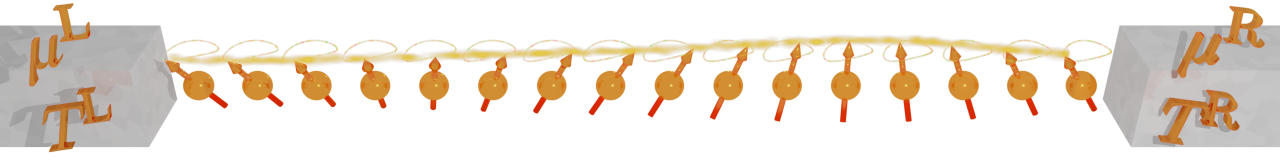
Figure 1: Cartoon representation of the system under consideration. A one-dimensional chain of spins is terminated at either end by heavy-metal leads, the left (right) lead having an electronic spin accumulation $\mu^{\mathrm{L(R)}}$ parallel to the magnetization axis, and temperature $T^{\mathrm{L(R)}}$. Spins precess elliptically due to the presence of high anisotropy, and can transport angular momentum in the form of an elliptical magnon or spin wave (yellow swirl).

We aim to consider systems typically used in long-distance transport experiments akin to Cornelissen et al. [7]: a ferromagnetic insulator with two heavy-metal leads, one of which serves to inject magnons, and one acting as a magnon detector. The system is biased by a constant electronic spin accumulation in the leads, aligned parallel to the magnetization so that there is no torque acting on the magnetization. We assume spin transport in the ferromagnetic insulator is quasi-one-dimensional, i.e., that magnons travel in a straight line from emitter to detector, and the bulk of the ferromagnet effectively consists of macroscopically many non-interacting parallel copies of the spin chain making up the transport channel for a single magnon. This allows us to treat the ferromagnetic bulk as a one-dimensional (1D) spin chain. A cartoon representation of this system is shown in Fig. 1. Extension to a two- or three-dimensional cubic bulk is mathematically simple (and tractable in the continuum limit), but computationally challenging for finite-sized systems due to the vast increase in lattice sites that must be taken into account.

We thus model our system using the 1D, $N$-particle Heisenberg [18] ferromagnetic insulator in the presence of quadratic anisotropy terms. It is described by the Hamiltonian

$$H =H_{\text{H}}+H_{\text{ani}},$$ (1)

where

$$H_{\text{H}} =-\frac{\tilde{J}}{2}\sum_{i=1}^{N-1}\bm{\hat{S}}_{i}\cdot\bm{\hat{S}}_{i+1}-h_{\mathrm{mag}}\sum_{i=1}^{N}\hat{S}_{i}^{z}$$ (2)

is the ordinary 1D Heisenberg Hamiltonian [18], and

$$H_{\text{ani}} =\sum_{\nu\in\{x,y,z\}}\sum_{i=1}^{N}K_{\nu}(\hat{S}^{\nu}_{i})^{2}$$ (3)

is the anisotropy Hamiltonian. Here $\tilde{J}>0$ is the exchange constant, the $K_{\nu}$ are the anisotropy energies in the three Cartesian directions, $\hat{\bm{S}}_{i}=(\hat{S}^{x}_{i},\hat{S}^{y}_{i},\hat{S}^{z}_{i})^{\mathrm{T}}$ is the spin operator at site $i$, and $h_{\mathrm{mag}}$ is an externally applied magnetic field.

As we are only interested in the behavior of the ferromagnet, we have omitted Hamiltonian terms originating from coupling to the leads, and instead opt to directly write down the relevant self-energy terms when we develop our Green’s function formalism later on.

The second-order, spin-$S$ Holstein-Primakoff transformation [17]

$$\hat{S}^{x}_{i} =\sqrt{\frac{S}{2}}\left(b_{i}+b^{\dagger}_{i}\right),$$ (4a)

$$\hat{S}^{y}_{i} =-\mathrm{i}\sqrt{\frac{S}{2}}\left(b_{i}-b^{\dagger}_{i}\right),$$ (4b)

$$\hat{S}^{z}_{i} =S-b^{\dagger}_{i}b_{i}$$ (4c)

is used to express the Hamiltonian 1 in terms of magnon creation (annihilation) operators $b^{\dagger}_{i}$ ($b_{i}$) acting at site $i$, that obey the bosonic commutation relations $[b_{i},b_{j}]=[b^{\dagger}_{i},b^{\dagger}_{j}]=0$ and $[b_{i},b^{\dagger}_{j}]=\delta_{ij}$. We additionally define the vector operator

$$\phi_{i} \equiv\begin{pmatrix}b_{i}\\ b^{\dagger}_{i}\end{pmatrix}$$ (5)

and its conjugate transpose $\phi^{\dagger}_{i}$.

Note that the Holstein-Primakoff transformation is an expansion around the ground state in which all spins are aligned in the $z$-direction. In the absence of an external field, this puts constraints on the relative signs and strengths of the anisotropy terms $K_{\nu}$, however a sufficiently strong field $h_{\mathrm{mag}}>0$ may always be used to guarantee alignment to the $z$-axis.

The Hamiltion of Eq. (1) may be simplified somewhat if one defines the constants $\Delta\equiv S(K_{x}+K_{y}-2K_{z}+\tilde{J})+h_{\mathrm{mag}}$, $J\equiv\frac{\tilde{J}S}{2}$ and $K\equiv\frac{S}{4}(K_{x}-K_{y})$. Then, dropping unimportant constant energy shifts, along with the additional boundary terms $-J(b^{\dagger}_{1}b_{1}+b^{\dagger}_{N}b_{N})$ that originate from the fact that we consider a finite-sized system (which we expect to be negligible for sufficiently large systems), the Hamiltonian (1) may be rewritten as

$$H =\frac{1}{2}\sum_{ij}\phi^{\dagger}_{i}h_{ij}\phi_{j},$$ (6)

with the $$2N\times 2N$$ matrix

$$h_{ij} =\begin{pmatrix}h^{\mathrm{i}}_{ij}&K\delta_{ij}\\ K\delta_{ij}&h^{\mathrm{i}}_{ij}\end{pmatrix}.$$ (7)

Here $$\delta_{ij} N\times N$$ is the identity matrix, and

$$h^{\mathrm{i}}_{ij} =\Delta\delta_{ij}-J\left[\delta_{i,j+1}+\delta_{i+1,j}\right]$$ (8)

is the isotropic Hamiltonian submatrix. We thus see that $\Delta$ is an on-site potential for the magnons. The rescaled exchange energy $J$ is a hopping parameter, governing the probability for a magnon to hop from one site to the next.

The off-diagonal submatrices $K\delta_{ij}$ govern the ellipticity of the magnons, and we shall henceforth use the term “the anisotropy” interchangeably with “the scalar constant $K$” (alternatively, and equivalently, $K$ could be called the “squeezing factor” or “spin nonconservation factor”). Note, however, that $K$ is proportional to the difference in anisotropy energies in the $x$ and $y$ directions, i.e. the principal directions perpendicular to the spin quantization axis.

The presence of nonzero $K$ breaks conservation of spin by introducing terms of the form $K\big{[}b_{i}b_{i}+b_{i}^{\dagger}b_{i}^{\dagger}\big{]}$. The Hamiltonian of Eq. (7) therefore cannot be unitarily diagonalized (in a physically meaningful way), and its eigenstates do not have a well-defined spin. Rather, Eq. (7) describes a Hamiltonian of the Bogoliubov form, which may be diagonalized using a para-unitary transformation [31], i.e. a transformation matrix $\mathcal{T}_{ij}$ obeying

$$\sum_{i}(\sigma_{3})_{ij}\mathcal{T}^{\dagger}_{jk} =\sum_{i}\mathcal{T}^{-1}_{ij}(\sigma_{3})_{jk},$$ (9)

where

$$(\sigma_{3})_{ij} \equiv\begin{pmatrix}\delta_{ij}&0\\ 0&-\delta_{ij}\end{pmatrix}$$ (10)

is the $$2N\times 2N \mathcal{T}_{ij}$$ analog of the third Pauli matrix (referred to as the para-identity matrix by Colpa [31]). The Hamiltonian (7) allows us to choose to be real, such that it takes the simple block structure

$$\mathcal{T}_{ij} =\begin{pmatrix}\mathcal{T}^{(1)}_{ij}&\mathcal{T}^{(2)}_{ij}\\ \mathcal{T}^{(2)}_{ij}&\mathcal{T}^{(1)}_{ij}\end{pmatrix},$$ (11)

where the individual $N\times N$ blocks $\mathcal{T}^{(1)}_{ij}$ and $\mathcal{T}^{(2)}_{ij}$ are not symmetric.

The para-unitary diagonalization of $h_{ij}$ is performed analytically for arbitrary $N\geq 2$ by leveraging the recurrent structure of the characteristic equation $\det\{h_{ij}-(\sigma_{3})_{ij}\varepsilon\}=0$, whereby the $N$-level equation can be expressed terms of the $(N-1)$- and $(N-2)$-level equations. The characteristic polynomial of the recurrence relation contains only terms of degree $N+1$, and is therefore easily solved analytically. The quasiparticles are elliptical magnons with the dispersion relation

$$\varepsilon_{n} =\sqrt{\left[\Delta-2J\cos\left(\frac{n\uppi}{N+1}\right)\right]^{2}-K^{2}}, 1 \leq n\leq N.$$ (12)

Here, the natural number $n$ is the quantum number, and $\varepsilon_{n}$ monotonically increases with $n$. The corresponding eigenstates are plane waves , with the quantum number $n$ corresponding to the wavenumber $k=\frac{n\uppi}{L}=\frac{n\uppi}{Na}$ for a spin chain of physical length $L=Na$, with $a$ the lattice constant.

II.2 Non-equilibrium Green’s function formalism

As stated in the previous subsection, diagonalization of our anisotropic ferromagnetic insulator Hamiltonian may be done analytically and results in free elliptical magnon modes. We now seek to investigate the finite-temperature steady-state behavior of such a system in the presence of two effects: (1) coupling to one or more metallic leads and (2) bulk dissipation of elliptical magnons in the form of Gilbert-like damping.

To this end, we develop a non-equilibrium Green’s function framework [33], also known as Keldysh formalism [23, 24]. In what follows, we set $\hbar=1$. The spectral properties of the magnons are encoded in the single-particle retarded Green’s function

$$g_{ij}(t,t^{\prime}) =-\mathrm{i}\theta(t-t^{\prime})\left<\left[\phi_{i}(t),\phi^{\dagger}_{j}(t^{\prime})\right]\right>$$ (13)

and advanced Green’s function

$$g^{\dagger}_{ij}(t,t^{\prime}) =\mathrm{i}\theta(t^{\prime}-t)\left<\left[\phi_{i}(t),\phi^{\dagger}_{j}(t^{\prime})\right]\right>,$$ (14)

where $$\theta(t-t^{\prime}) [\bullet,\bullet]$$ is the Heaviside step function and is the commutator. The Keldysh Green’s function

$$g^{\mathrm{K}}_{ij}(t,t^{\prime}) =-\mathrm{i}\left<\left\{\phi_{i}(t),\phi^{\dagger}_{j}(t^{\prime})\right\}\right>$$ (15)

encodes information about the occupation of the single-particle states. Here, $$\{\bullet,\bullet\}$$ is the anticommutator. Using these Green’s functions, one may construct the lesser Green’s function

$$g^{<}_{ij}(t,t^{\prime}) =-\mathrm{i}\left<\phi^{\dagger}_{i}(t)\phi_{j}(t^{\prime})\right>,$$ (16)

which, at equal times $$t=t^{\prime} i\neq j i=j -\mathrm{i}$$, contains the off-diagonal correlations (for ) and quasiparticle number density (for ), up to a prefactor of . Together with the greater Green’s function

$$g^{>}_{ij}(t,t^{\prime}) =-\mathrm{i}\left<\phi_{i}(t)\phi^{\dagger}_{j}(t^{\prime})\right>,$$ (17)

one obtains the relations [24]

$$g_{ij}(t,t^{\prime}) =\theta(t-t^{\prime})\left[g^{>}_{ij}(t,t^{\prime})-g^{<}_{ij}(t,t^{\prime})\right],$$ (18)

$$g^{\dagger}_{ij}(t,t^{\prime}) =-\theta(t^{\prime}-t)\left[g^{>}_{ij}(t,t^{\prime})-g^{<}_{ij}(t,t^{\prime})\right],$$ (19)

$$g^{\mathrm{K}}_{ij}(t,t^{\prime}) =g^{>}_{ij}(t,t^{\prime})+g^{<}_{ij}(t,t^{\prime}),$$ (20)

and

$$g_{ij}(t,t^{\prime})-g^{\dagger}_{ij}(t,t^{\prime}) =g^{>}_{ij}(t,t^{\prime})-g^{<}_{ij}(t,t^{\prime}).$$ (21)

For simplicity, we shall henceforth drop the subscripts $i,j,\dotsc$ on all matrices, as well as the explicit summations in matrix products seen in Section II.1, and work in the space of $2\times 2$ matrices, of which the four components are themselves $N\times N$ matrices. The presence of the $N\times N$ or $2N\times 2N$ identity matrix is implied when doing so does not lead to ambiguity.

For the remainder of this work, we shall only consider a system in the steady state, i.e. $g(t,t^{\prime})=g(t-t^{\prime})$ (and similar for the other Green’s functions), and work with Fourier-transformed Green’s functions. In particular, the retarded Green’s function $g(\omega)$ satisfies the Dyson equation

$$g(\omega) =[\omega\sigma_{3}-h-\Sigma(\omega)]^{-1},$$ (22)

where $\Sigma(\omega)$ is the retarded self-energy, and is easily obtained by numerical matrix inversion.

Here, we opt to stay in the HP basis (i.e., the basis of the circular magnons defined by the operators $\phi$ and $\phi^{\dagger}$) instead of transforming to the elliptical basis, and thus $h$ in Eq. (22) is simply given by Eq. (7). Lead coupling and Gilbert-like damping are to be incorporated into the (retarded) self-energy $\Sigma$.

The reason we choose to compute observables in the circular basis is twofold: (1) it provides a simple form for the lead self-energies, which will be explained shortly, and (2) experimental measurement of observables is generally done electrically (through the spin Hall effect and its inverse) [7, 34], so that electron spin is the natural measurement basis (see below).

In line with Zheng et al. [14], we take the self-energy component arising from lead $X$ to have the form

$$\Sigma^{X}(\omega) =-\mathrm{i}\eta^{X}(\omega-\mu^{X}\sigma_{3})\delta_{i,i^{X}}\delta_{j,i^{X}},$$ (23)

where $\delta_{i,i^{X}}\delta_{j,i^{X}}$ indicates that the self-energy is zero everywhere except for its diagonal components corresponding to site $i^{X}$, i.e. the index where lead $X$ is attached. The positive dimensionless real constant $\eta^{X}$ determines the strength of the lead’s coupling to the system, and $\mu^{X}$ is the spin accumulation—i.e. the difference in chemical potential between spin-up and spin-down electrons—in the lead, generated, for example, by the spin Hall effect. In this work, we attach at most two leads: the left lead ($X=\mathrm{L}$) at $i^{\mathrm{L}}=1$ and optionally the right lead ($X=\mathrm{R}$) at $i^{\mathrm{R}}=N$. We choose the coupling for positive and negative modes to be equal-but-opposite [indicated by $\mu^{X}\sigma_{3}$ in Eq. (23)], such that our system reduces to the one considered by Zheng et al. [14] in the limit $K\to 0$ (up to the splitting into positive and negative modes itself, which, at $K=0$, becomes a purely notational operation). At the level of the approximations used by Zheng et al. [14], the lead self-energy for this geometry is determined only by the electrons in the metal and the interfacial interaction, and is independent of the magnons and their particle-hole structure, making the form of Eq. (23) a natural choice for our model.

The form of the lead self-energy given by Eq. (23) is only valid when one assumes the spin basis is the natural basis for the lead Hamiltonians, i.e., that the leads inject a well-defined amount of spin into the ferromagnet. This is the case provided the electron spin in the leads is polarized in the $z$-direction and a spin-flip scattering process at the interface is the source of magnons: here a spin-$\frac{1}{2}$ excitation in the leads is flipped to $-\frac{1}{2}$, injecting a (spin-1) HP magnon into the ferromagnet. In the presence of anisotropy, the circular HP magnon is a superposition of elliptical magnons.

To find an expression for the Gilbert-like damping self-energy, it is important to carefully consider what one would expect the state of the system to be in thermal equilibrium. Given that the lead contributions are local, acting on only one or two sites of a much larger bulk, we assume our system ultimately thermalizes to states close to the eigenstates of the free anisotropic ferromagnet, i.e. the elliptical quasiparticles. Thus, what is linearly damped in our system is the density of elliptical magnons, which does not necessarily correspond to the classical magnetization—hence our use of the term ‘Gilbert-like damping’, as opposed to just ‘Gilbert damping’: the latter, in the strict sense, refers to damping of the classical magnetization only [36].

By this rationale, we employ a simple linear damping self-energy in the elliptical basis:

$$\Sigma^{\mathrm{B,ell}} =-\mathrm{i}\alpha\omega.$$ (24)

Here $\mathrm{B}$ stands for ‘bulk’ (as this is the only bulk self-energy we take into account), and $\alpha$ is the Gilbert-like damping parameter.

Transforming to the spin basis, we find

$$\Sigma^{\mathrm{B}}(\omega) =-\mathrm{i}\alpha\omega\mathcal{T}^{\dagger}\mathcal{T},$$ (25)

where $\mathcal{T}^{\dagger}\mathcal{T}$ becomes the identity matrix in the limit $K\to 0$. In this limit, the bulk self-energy reduces to standard Gilbert damping, which has been addressed by Zheng et al. [14].

The total (retarded) self-energy in our model is then simply the sum of the lead- and bulk self-energies in the spin basis:

$$\Sigma(\omega) =\Sigma^{\mathrm{B}}(\omega)+\Sigma^{\mathrm{L}}(\omega)+\Sigma^{\mathrm{R}}(\omega).$$ (26)

Under the assumption that the lead and bulk thermal baths are sufficiently large to be undisturbed by coupling to the spins, we may use the fluctuation-dissipation theorem [24] to find the associated Keldysh self-energy:

$$\Sigma^{\mathrm{K}}(\omega) =2\Sigma^{\mathrm{B}}(\omega)\mathcal{T}^{-1}F^{\mathrm{B}}(\omega)\mathcal{T}$$

$$\qquad+2\Sigma^{\mathrm{L}}(\omega)F^{\mathrm{L}}(\omega)+2\Sigma^{\mathrm{R}}(\omega)F^{\mathrm{R}}(\omega).$$ (27)

Here, we define the statistical matrix

$$F^{X}(\omega) \equiv\operatorname{diag}\Bigg{\{}\coth\left(\frac{\omega-\mu^{X}}{2k_{\mathrm{B}}T^{X}}\right),$$

$$\hskip 60.00009pt-\coth\left(\frac{-\omega-\mu^{X}}{2k_{\mathrm{B}}T^{X}}\right)\Bigg{\}},$$ (28)

with $X\in\{\mathrm{B},\mathrm{L},\mathrm{R}\}$, $k_{\mathrm{B}}$ the Boltzmann constant, and $T^{X}$ the temperature of the subsystem $X$. We will further assume the magnon chemical potential vanishes ($\mu^{\mathrm{B}}=0$), such that $\mathcal{T}^{-1}F^{\mathrm{B}}(\omega)\mathcal{T}=\coth\left(\frac{\omega}{2k_{\mathrm{B}}T^{\mathrm{B}}}\right)$ is a real number multiplying the identity matrix.

Finally, from the Keldysh self-energy, we compute the Keldysh Green’s function [23, 37]

$$g^{\mathrm{K}}(\omega) =g(\omega)\Sigma^{\mathrm{K}}(\omega)g^{\dagger}(\omega).$$ (29)

Note that $g^{\mathrm{K}}(\omega)$ is symmetric and anti-hermitian, and therefore pure-imaginary.

II.3 Observables

Using the elements outlined in Section II.2, we may compute any physical observable of our system. As we are primarily interested in steady-state behavior, the most obvious objects to consider are the equal-time two-point functions of the creation and annihilation operators of HP magnons. In the presence of anisotropy, we expect to obtain nonzero anomalous correlations, e.g. $\big{<}b_{i}b_{j}\big{>}$, because the states in the system are a superposition of HP magnon states (leading to nonconservation of spin). The normal and anomalous correlation functions are conveniently collected in a single matrix through the vector operator $\phi$, e.g.

$$\mathrm{i}g^{>}_{ij}(t) =\left<\phi_{i}(t)\phi^{\dagger}_{j}(t)\right>=\left<\begin{pmatrix}b_{i}(t)\\ b^{\dagger}_{i}(t)\end{pmatrix}\otimes\begin{pmatrix}b^{\dagger}_{j}(t)&b_{j}(t)\end{pmatrix}\right>$$

$$=\begin{pmatrix}\Big{<}b_{i}(t)b^{\dagger}_{j}(t)\Big{>}&\Big{<}b_{i}(t)b_{j}(t)\Big{>}\\ \Big{<}b^{\dagger}_{i}(t)b^{\dagger}_{j}(t)\Big{>}&\Big{<}b^{\dagger}_{i}(t)b_{j}(t)\Big{>}\end{pmatrix}.$$ (30)

Conversely, we may compute two-point functions of the elliptical magnons $\Psi\equiv\mathcal{T}\phi\equiv\begin{pmatrix}\psi,&\psi^{\dagger}\end{pmatrix}$, e.g.

$$\left<\Psi^{\dagger}(t)\Psi(t)\right> =\mathcal{T}^{*}\left<\phi^{\dagger}(t)\phi(t)\right>\mathcal{T}^{\mathrm{T}}.$$ (31)

Here, we expect the anomalous blocks to be nonzero only when lead coupling and anisotropy are simultaneously present: if only anisotropy is present, there are no damping terms that try to push the system away from the native elliptical magnon eigenstates (spin is not conserved, but there are no explicit sources and sinks of spin). Conversely, if lead coupling is present but anisotropy is absent, the elliptical magnons are identical to the HP ones, there is no breaking of spin conservation, and the system reduces to the case investigated by Zheng et al. [14].

As stated in Section II.2, the matrix $\rho_{\mu\nu}=\big{<}\phi^{\dagger}_{\mu}\phi_{\nu}\big{>}$ (at some arbitrary time in the steady state, and with the indices $\mu$ and $\nu$ in the range $[1,2N]$) containing number densities and off-diagonal correlations may be computed through the lesser Green’s function $g^{<}$:

$$\rho=\mathrm{i}g^{<} =\mathrm{i}\int\frac{\mathrm{d}\omega}{2\uppi}\,g^{<}(\omega)$$ (32)

$$=\frac{\mathrm{i}}{2}\int\frac{\mathrm{d}\omega}{2\uppi}\,\left(g^{\mathrm{K}}(\omega)-g(\omega)+g^{\dagger}(\omega)\right).$$

For the sake of brevity, we shall refer to $\rho$ as the density matrix, although the off-diagonal components are in fact off-diagonal correlations. Note also that by the symmetry of $g$ and $g^{\mathrm{K}}$, and anti-hermiticity of the Keldysh Green’s function, the lesser Green’s function is itself symmetric, anti-hermitian and pure-imaginary. One may alternatively work directly with the Keldysh Green’s function, of which the corresponding observable is the semiclassical (SC) HP magnon density matrix

$$\rho^{\mathrm{SC}}=\frac{\mathrm{i}}{2}g^{\mathrm{K}}-\frac{1}{2} =\frac{1}{2}\left<\left\{\phi^{\dagger},\phi\right\}\right>-\frac{1}{2}$$

$$=\frac{\mathrm{i}}{2}\int\frac{\mathrm{d}\omega}{2\uppi}\,g^{\mathrm{K}}(\omega)-\frac{1}{2}.$$ (33)

In equilibrium, the top-left and off-diagonal blocks correspond directly to those of the true density matrix of Eq. (32).

From the density matrix $\rho$, we may compute the uncertainty operators $\Delta\bar{S}^{x}$ and $\Delta\bar{S}^{y}$ for the corresponding normalized spin operators $\bar{S}^{x}$ and $\bar{S}^{y}$, which allow us to determine whether the elliptical magnons are squeezed in phase space [26]. From the normalized spin operators

$$\bar{S}^{x}_{i} =\frac{1}{\sqrt{2}}\left(b_{i}+b^{\dagger}_{i}\right),$$ (34a)

$$\bar{S}^{y}_{i} =\frac{-\mathrm{i}}{\sqrt{2}}\left(b_{i}-b^{\dagger}_{i}\right),$$ (34b)

and

$$\bar{S}^{z}_{i} =1-b^{\dagger}_{i}b_{i},$$ (34c)

[i.e. the HP transformation with $S$ set to 1, and applied in reverse with respect to Eqs. (4)], we immediately find the uncertainty operators

$$\Delta\bar{S}^{x}_{i} \equiv\sqrt{\big{<}(\bar{S}^{x}_{i})^{2}\big{>}-\big{<}\bar{S}^{x}_{i}\big{>}^{2}}$$

$$=\sqrt{\frac{1}{2}\left[\big{<}b_{i}b^{\dagger}_{i}\big{>}+\big{<}b^{\dagger}_{i}b_{i}\big{>}+\big{<}b_{i}b_{i}\big{>}+\big{<}b^{\dagger}_{i}b^{\dagger}_{i}\big{>}\right]}$$

$$=\sqrt{\frac{1}{2}\left[I_{+}\rho I_{+}^{\mathrm{T}}\right]_{ii}}$$ (35a)

and

$$\Delta\bar{S}^{y}_{i} \equiv\sqrt{\big{<}(\bar{S}^{y}_{i})^{2}\big{>}-\big{<}\bar{S}^{y}_{i}\big{>}^{2}}$$

$$=\sqrt{\frac{1}{2}\left[\big{<}b_{i}b^{\dagger}_{i}\big{>}+\big{<}b^{\dagger}_{i}b_{i}\big{>}-\big{<}b_{i}b_{i}\big{>}-\big{<}b^{\dagger}_{i}b^{\dagger}_{i}\big{>}\right]}$$

$$=\sqrt{\frac{1}{2}\left[I_{-}\rho I_{-}^{\mathrm{T}}\right]_{ii}},$$ (35b)

where $$I_{\pm} N\times 2N$$ are the matrices

$$I_{\pm} \equiv\delta_{ij}(1,\pm 1).$$ (35c)

Here, the one-point functions $\big{<}\bar{S}^{x}_{i}\big{>}$ and $\big{<}\bar{S}^{y}_{i}\big{>}$ vanish, because we do not explicitly couple to a pumping field and are not considering Bose-Einstein condensates [19]. The Robertson uncertainty principle [38] then states that $\Delta\bar{S}^{x}_{i}\Delta\bar{S}^{y}_{i}\geq\frac{1}{2}$. If either $\Delta\bar{S}^{x}_{i}<\frac{1}{\sqrt{2}}$ or $\Delta\bar{S}^{y}_{i}<\frac{1}{\sqrt{2}}$, the state is squeezed [26], and the pattern of quantum fluctuations of the spin around the $z$-axis takes the form of an ellipse, rather than a circle [20]. As noted by Kamra et al. [20], the purely quantum mechanical squeezing should not be confused with the magnetization trajectory of a classical elliptical spin wave: the latter concerns coherent excited states, whereas squeezing persists even in the ground state and affects properties such as entanglement.

In addition to the magnon density and the related observables, we may compute the spin currents in our system. These follows from the continuity equation of the magnetization; a brief outline of the derivation is given in Appendix A. The total spin current $j_{\mathrm{s,tot}}^{\mathrm{L}}$ flowing out of the left lead comprises three Landauer-Büttiker-type [39] terms:

$$j_{\mathrm{s,tot}}^{\mathrm{L}}(t) =j_{\mathrm{s}}^{\mathrm{R}\to\mathrm{L}}+j_{\mathrm{s}}^{\mathrm{B}\to\mathrm{L}}+j_{\mathrm{s}}^{\mathrm{L}}$$ (36)

where

$$j_{\mathrm{s}}^{X} =-\operatorname{Re}\operatorname{Tr}\int\frac{\mathrm{d}\omega}{2\uppi}\iota^{X}(\omega).$$ (37)

Here the integrands $\iota^{X}$ are the tunneling term

$$\iota^{\mathrm{R}\to\mathrm{L}}(\omega) =g^{\dagger}(\omega)\sigma_{3}\Sigma^{\mathrm{L}}(\omega)g(\omega)\Sigma^{\mathrm{R}}(\omega)$$

$$\hskip 50.00008pt\times\left[F^{\mathrm{R}}(\omega)-F^{\mathrm{L}}(\omega)\right],$$ (38a)

the bulk term

$$\iota^{\mathrm{B}\to\mathrm{L}}(\omega) =g^{\dagger}(\omega)\sigma_{3}\Sigma^{\mathrm{L}}(\omega)g(\omega)\Sigma^{\mathrm{B}}(\omega)$$

$$\hskip 50.00008pt\times\left[\mathcal{T}^{-1}F^{\mathrm{B}}(\omega)\mathcal{T}-F^{\mathrm{L}}(\omega)\right],$$ (38b)

and the lead-local term

$$\iota^{\mathrm{L}}(\omega) =g^{\dagger}(\omega)\sigma_{3}\Sigma^{\mathrm{L}}(\omega)g(\omega)h$$

$$\hskip 50.00008pt\times\left[\left.F^{\mathrm{L}}(\omega)\right|_{\mu^{\mathrm{L}}=0}-F^{\mathrm{L}}(\omega)\right].$$ (38c)

Conversely, the spin current out of the right lead consists of the same expressions but with $\mathrm{L}$ and $\mathrm{R}$ swapped.

Note that the terms in $j_{\mathrm{s,tot}}^{\mathrm{L}}$ contain the statistical matrices $F^{X}(\omega)$ in place of the scalar Bose-Einstein functions one would normally find in Landauer-Büttiker equations. One may exploit various symmetries of the components of the integrals to recover the more familiar form (in the circular limit identical to the expressions given by Zheng et al. [14]), though this requires the transmission functions to be written in terms of the individual $N\times N$ blocks of the component $2N\times 2N$ matrices, as has been done by e.g. Rückriegel and Duine [29].

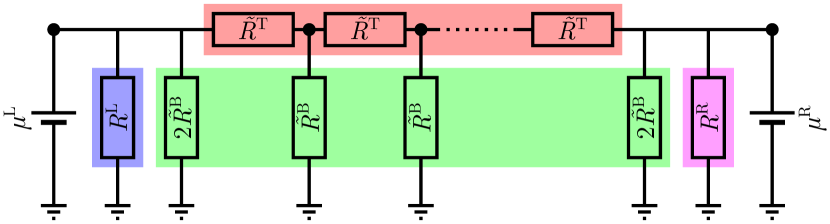
(a)

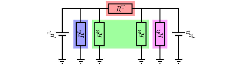
(b)

Figure 2: Resistor network diagrams of our model system. LABEL:sub@fig:resnetwork-full: In the full diagram, each black dot represents a spin, each resistor $\tilde{R}^{\mathrm{T}}$ represents an inter-spin coupling, and each resistor $\tilde{R}^{\mathrm{B}}$ represents a coupling to the field(s) responsible for Gilbert-like damping. The spin currents through the resistors $R^{\mathrm{L/R}}$ are given by the lead-local terms $-j^{\mathrm{L/R}}$. LABEL:sub@fig:resnetwork-reduced: By repeated application of the $\Delta-Y$ transform [40], one may collapse the internal couplings (red and green blocks), thereby reducing the $N$-spin resistor network to a five-resistor form. In this reduced diagram, the current through $R^{\mathrm{T}}$ (from right to left) is given by $j^{\mathrm{R\to L}}$ and the currents through the left (right) resistors $R^{\mathrm{B}}$ are represented by the bulk terms $-j^{\mathrm{B\to L(R)}}$. The lead-local resistors remain unchanged.

To interpret the three spin current contributions, it is useful to consider the system as a spin resistor network, shown in Fig. 2a. Here each node in the circuit represents a spin in our chain, and each resistor represents a coupling either between spins (tunneling resistors $\tilde{R}^{\mathrm{T}}$) or to a damping element (Gilbert-like damping for the bulk resistors $\tilde{R}^{\mathrm{B}}$, and lead damping for $R^{\mathrm{L/R}}$). The system is biased at either lead with a spin accumulation (voltage) $\mu^{\mathrm{L/R}}$. In this resistor network analogy, one may ‘integrate out’ the bulk spins by repeated application of the $\Delta-Y$ transform [40] to obtain Fig. 2b. At equal temperature ($T^{\mathrm{L}}=T^{\mathrm{R}}=T^{\mathrm{B}}=T$), the spin currents $j^{\mathrm{X}}$ may then be interpreted as follows:

The tunneling term $j^{\mathrm{R\to L}}$ is the current flowing from right to left through the resistor $R^{\mathrm{T}}$ in Fig. 2b, and corresponds to the spin current flowing out of the left lead when a spin accumulation is applied at the right lead. Physically, it is the term corresponding to magnon-mediated non-local transport, and roughly corresponds to the current measured experimentally in a ferromagnetic insulator by Cornelissen et al. [7], although our work considers the ballistic regime ($\mu^{\mathrm{B}}=0$) rather than the diffusive regime.

The bulk term $j^{\mathrm{B\to L}}$ corresponds to the current flowing out of the left lead as a result of Gilbert-like damping in the bulk. It is negative when a positive spin accumulation is applied to the left lead, indicating spin current flows from the lead into the bulk, where it is dissipated into the lattice. In Fig. 2b, $-j^{\mathrm{B\to L(R)}}$ is the current flowing to ground through the left (right) resistor $R^{\mathrm{B}}$.

The lead-local term $j^{\mathrm{L}}$, corresponding to the current flowing from ground upwards through $R^{\mathrm{L}}$ in Fig. 2b, is unique to systems that exhibit the Bogoliubov structure described at the start of this section. It is linear in $K$ to lowest nonvanishing order, and, at nonzero $K$, vanishes unless the system is driven by the application of an electronic spin accumulation in the lead. We may therefore conclude that it arises due to the mismatch between the lead states, where spin is a good quantum number, and the elliptical magnon eigenstates of the anisotropic ferromagnet. Ultimately, the mismatch is necessarily compensated by the lattice [21]. As this term contributes directly to the spin current flowing out of the lead to which a spin bias is applied, it offers a way to probe the ellipticity of magnons through local spin current measurements.

Taking the resistor network analogy further, the reduced model of Fig. 2b provides us with a new set observables more generic than the spin currents themselves, namely the spin resistances $R^{\mathrm{T}}$, $R^{\mathrm{L/R}}$ and $R^{\mathrm{B}}$. Setting $\mu^{\mathrm{R}}=0$ and formally expanding the left-lead spin current terms in $\mu^{\mathrm{L}}$, we obtain

$$j_{\mathrm{s}}^{\mathrm{R\to L}} =j_{\mathrm{s0}}^{\mathrm{R\to L}}(T^{\mathrm{L}},T^{\mathrm{R}})-\frac{1}{R^{\mathrm{T}}}\mu^{\mathrm{L}},$$ (39a)

$$j_{\mathrm{s}}^{\mathrm{B\to L}} =j_{\mathrm{s0}}^{\mathrm{B\to L}}(T^{\mathrm{L}},T^{\mathrm{B}})-\frac{1}{R^{\mathrm{B}}}\mu^{\mathrm{L}},$$ (39b)

$$j_{\mathrm{s}}^{\mathrm{L}} =-\frac{1}{R^{\mathrm{L}}}\mu^{\mathrm{L}}.$$ (39c)

Here $j_{\mathrm{s0}}^{\mathrm{R\to L}}(T^{\mathrm{L}},T^{\mathrm{R}})$ and $=j_{\mathrm{s0}}^{\mathrm{B\to L}}(T^{\mathrm{L}},T^{\mathrm{B}})$ are spin Seebeck effect [41, 12] terms that vanish when $T^{\mathrm{L}}=T^{\mathrm{R}}$ and $T^{\mathrm{L}}=T^{\mathrm{B}}$, respectively.

III Numerical implementation and results

The framework outlined in the previous section is implemented numerically for system sizes of order $N=20$. At low or moderate damping, the functions in our setup are sharply peaked in the frequency domain; frequency integrals are evaluated with an adaptive trapezoidal algorithm to avoid missing such peaks. As the setup requires matrices of size $2N\times 2N$ and the computation of observables includes one matrix inversion and multiple dense matrix multiplications per frequency sample, the numerical implementation scales poorly with system size. However, as the qualitative differences between systems of size $N=40$ and $N=20$ turn out to be minimal, we believe the latter to be a fair compromise between manageable computation time and sufficient capture of large-system behavior.

Our use of simplistic linear damping leads to a logarithmic divergence if the frequency integrals in the expressions for $\rho$ or $\rho^{\mathrm{SC}}$ are taken from $-\infty$ to $\infty$. We regularize the integrals by restricting the integration interval to $[-\varepsilon_{\mathrm{max}},\varepsilon_{\mathrm{max}}]$, where

$$\varepsilon_{\mathrm{max}} =\lim_{N\to\infty}\varepsilon_{N}.$$ (40)

We seek to investigate qualitative changes in the behavior of our system as the anisotropy $K$ is increased, while mitigating the effects of changes to the energetics of the ferromagnet’s eigenstates. To realize this, we shall keep the elliptical magnon gap $\varepsilon_{1}$, given by Eq. (12), fixed. Furthermore, we keep the exchange-like constant $J$ fixed, and adjust the field-like parameter $\Delta=2J\cos\left(\frac{\uppi}{N+1}\right)+\sqrt{\varepsilon_{1}^{2}+K^{2}}$ accordingly. Finally, we shall measure all energy scales relative to $J$, which is numerically realized by setting $J=1$.

III.1 Spin conductances

We compute the spin conductances

$$G^{\mathrm{T}} \equiv\frac{1}{R^{\mathrm{T}}},$$ (41a)

$$G^{\mathrm{B}} \equiv\frac{1}{R^{\mathrm{B}}},$$ (41b)

and

$$G^{\mathrm{L}} \equiv\frac{1}{R^{\mathrm{L}}}$$ (41c)

by fitting the components of $j_{\mathrm{s,tot}}^{\mathrm{L}}$ to Eqs. (39) for small values of $\mu^{\mathrm{L}}$, setting $T^{\mathrm{L}}=T^{\mathrm{R}}=T^{\mathrm{B}}=T$ and $\mu^{\mathrm{R}}=0$. We consider a system with parameters $N=20$, $\alpha=0.001$, $\varepsilon_{1}=0.025J$ and $\eta^{\mathrm{L}}=\eta^{\mathrm{R}}=8$. (Here, the values for $\eta^{\mathrm{L/R}}$ are chosen in line with Zheng et al. [14], while our choices for $\alpha$ and $\varepsilon_{1}$ are fairly arbitrary within the low-damping and low-gap regimes, respectively.) Note that because we have set $\hbar=1$, the conductances are dimensionless.

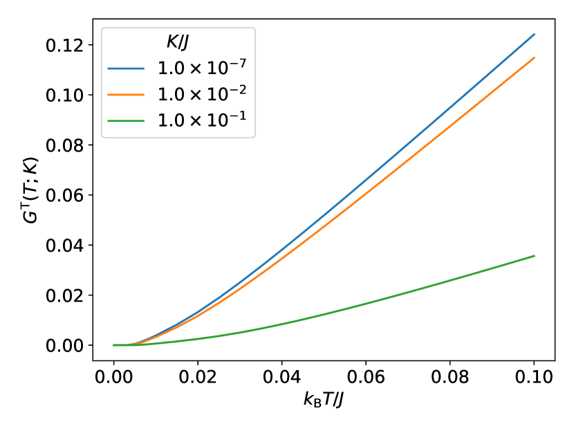
Figure 3: Tunneling conductance versus temperature at magnon gap $\varepsilon_{1}/J=0.025$, for different values of the anisotropy $K$.

Figure 3 shows the tunneling conductance $G^{\mathrm{T}}$ vs. temperature $k_{\mathrm{B}}T$ at various values of $K$. In all cases, the tunneling conductance vanishes at $T=0$ (to numerical accuracy; the highly nonlinear behavior at low temperature limits the fitting accuracy) and slowly transitions to being linear with temperature. The effect of anisotropy is to suppress the conductance, although this effect is small until $K/J=\mathcal{O}(0.1)$, i.e. very large anisotropy (e.g. for yttrium-iron garnet, a comparison of literature values [42, 43, 44, 45, 46] yields $K/J=\mathcal{O}(10^{-3}\text{---}10^{-2})$, although the range is highly variable between different materials [47]). Physically, this may be understood by the fact that the leads are not commensurate to the elliptical spin waves, which causes an increase in reflection at the interface.

The bulk conductance $G^{\mathrm{B}}$, shown in Fig. 4, similarly vanishes at $T=0$ and is suppressed by anisotropy. Unlike the tunneling conductance, where the transition to a linear regime is smeared out at higher anisotropies, the bulk conductance transitions more abruptly, at $k_{\mathrm{B}}T/J\sim 0.005$. The suppression with anisotropy is mild: at $k_{\mathrm{B}}T/J=0.1$, increasing the anisotropy from $K/J=$1\text{\times}{10}^{-7}$$ to $K/J=$1\text{\times}{10}^{-1}$$ suppresses the bulk conductance by roughly 8%. Our formalism does not elucidate the physical mechanism underlying this suppression, however, given its small magnitude, we believe it to be a natural consequence of the anisotropy-dependence of the dispersion, rather than being the result of any nontrivial effect.

The relatively abrupt transition to a linear regime is a direct consequence of the low-$\mu^{\mathrm{L}}$ behavior of the difference of statistical matrices in the bulk spin current integrand (38b):

$$\coth\left(\frac{\omega}{2k_{\mathrm{B}}T}\right) \mp\coth\left(\frac{\pm\omega-\mu^{\mathrm{L}}}{2k_{\mathrm{B}}T}\right)$$

$$\approx\pm\frac{\mu^{\mathrm{L}}}{k_{\mathrm{B}}T-k_{\mathrm{B}}T\cosh\left(\frac{\omega}{k_{\mathrm{B}}T}\right)}.$$ (42)

Given that the most significant contribution to $G^{\mathrm{B}}$ arises from a narrow region of $\iota^{\mathrm{B\to L}}$ centred around $\omega=\varepsilon_{1}$ (as one would expect), we may judiciously substitute $\omega=\varepsilon_{1}=0.025J$ in this expression. Dividing by $\mu^{\mathrm{L}}$, we then obtain a function that exhibits a kink near $k_{\mathrm{B}}T/J=0.005$, similar to the bulk conductance. We may thus conclude, qualitatively, that the kink is explained by the requirement for the temperature to overcome the finite gap.

In Fig. 5, it can be seen that the lead-local conductance $G^{\mathrm{L}}$ nearly vanishes at low anisotropy (as expected) and reaches a magnitude roughly comparable to the bulk conductance at the fairly high anisotropy value $K/J=$1\text{\times}{10}^{-2}$$. However, $G^{\mathrm{L}}$ is vastly enhanced at the very high anisotropy value $K/J=\mathcal{O}(0.1)$, becoming several times larger than the tunneling conductance, indicating most spin is lost to the lattice at the left-lead interface. This bears similarity to the appearance of evanescent spin waves in anisotropic systems [48], however, rigorously showing the relation between these effects requires reconstructing the classical wave picture from our formalism, which is beyond the scope of this work. Like the bulk conductance, the transition to a linear regime in the lead-local conductance is relatively abrupt for the $K/J=$1\text{\times}{10}^{-1}$$ curve.

Although the tunneling and bulk conductances are suppressed by increasing anisotropy, the corresponding increase in the lead-local conductance is greater than the decrease in the sum of tunneling and bulk conductances. In other words, the conductance of the parallel combination of the three spin resistors $R^{\mathrm{T}}$, $R^{\mathrm{B}}$ and $R^{\mathrm{L}}$ increases with increasing anisotropy, while the individual conductances of $R^{\mathrm{T}}$ and $R^{\mathrm{B}}$ decrease. Thus, although our model does not provide an obvious way to separate the bulk and lead-local contributions, it suggests the presence of anisotropy causes the local spin conductance to increase, while the nonlocal conductance decreases, thereby potentially providing an experimental way to probe the anisotropy of a ferromagnetic insulator using spin current measurements.

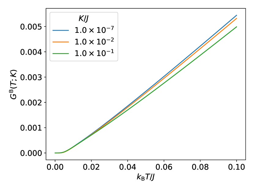
Figure 4: Bulk conductance versus temperature at magnon gap $\varepsilon_{1}/J=0.025$, for different values of the anisotropy $K$.

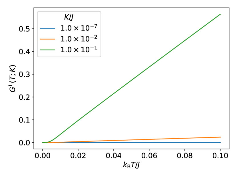
Figure 5: Lead-local conductance versus temperature at magnon gap $\varepsilon_{1}/J=0.025$, for different values of the anisotropy $K$.

III.2 Correlation functions and squeezing

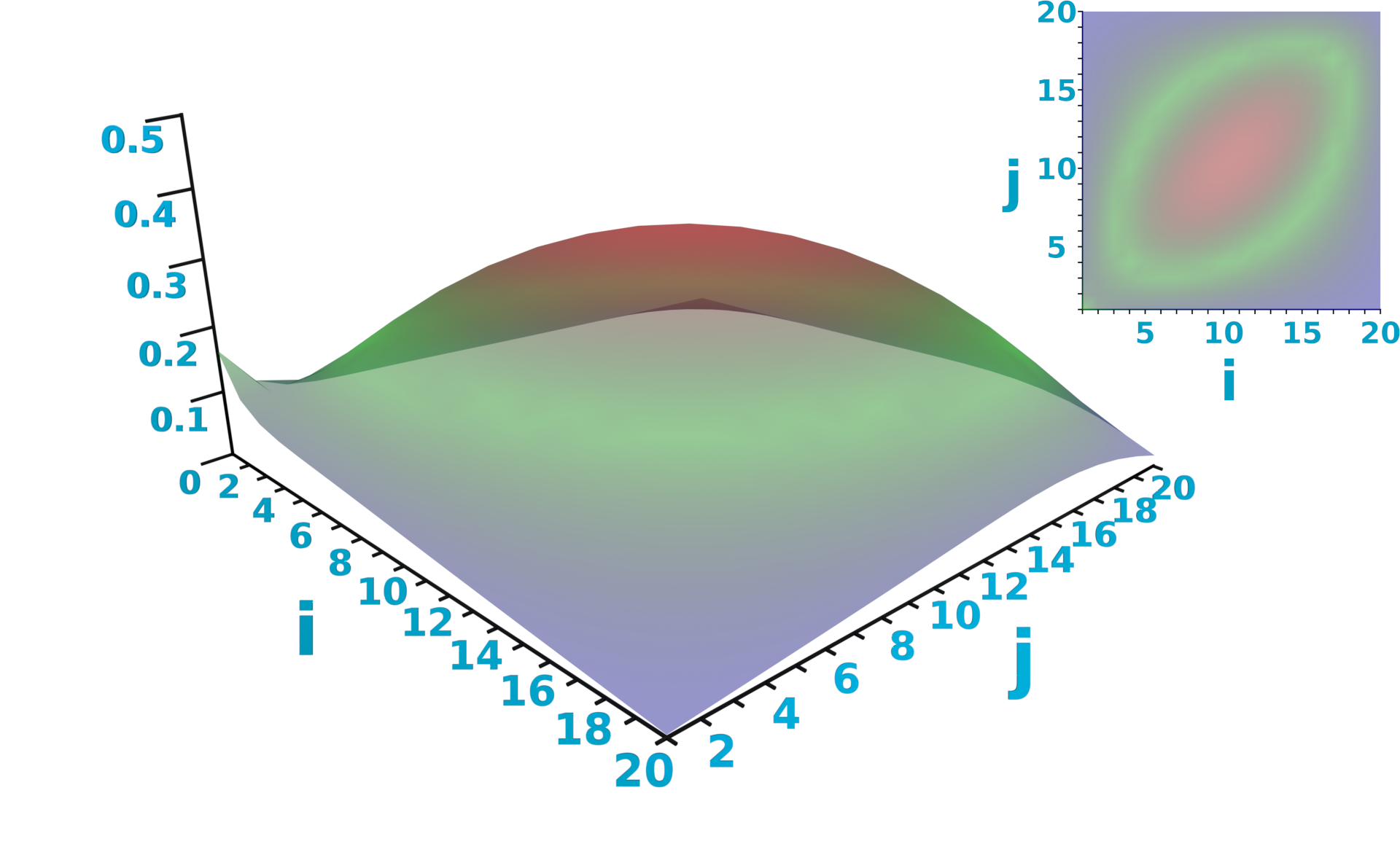
(a)

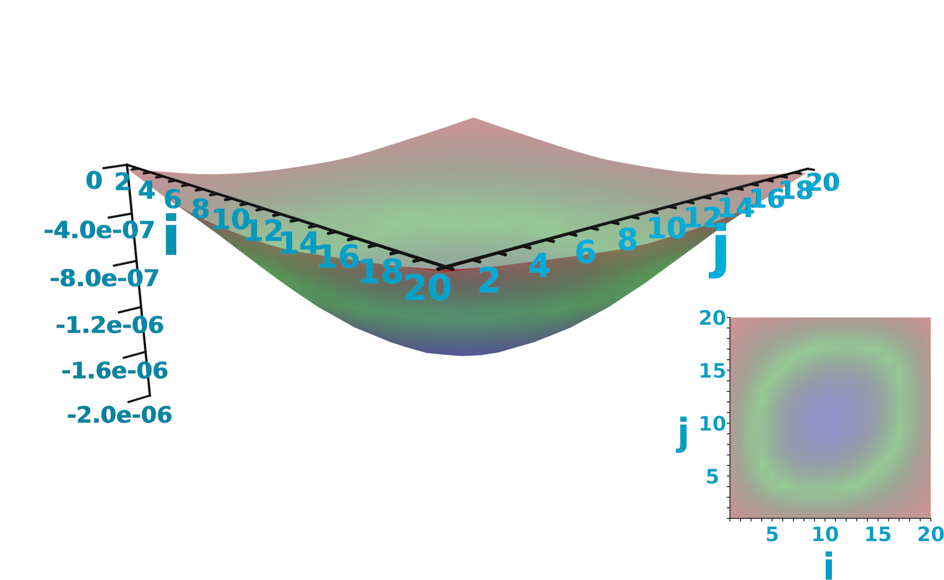
(b)

Figure 6: Normal and anomalous spin densities for a system of size $N=20$ with only the left lead attached ($\eta^{\mathrm{L}}=8$, $\eta^{\mathrm{R}}=0$), low Gilbert-like damping $\alpha=$1\text{\times}{10}^{-3}$$, temperature $T/J=0.1$, gap $\varepsilon_{1}/J=0.025$, and anisotropy $K/J=$1\text{\times}{10}^{-7}$$. The horizontal axes represent the site indices $i$ and $j$. Insets: heatmaps of the corresponding 3D plots. LABEL:sub@fig:rholesser1a: normal density $\big{<}b^{\dagger}_{i}(t)b_{j}(t)\big{>}$. LABEL:sub@fig:rholesser1b: anomalous density $\big{<}b^{\dagger}_{i}(t)b^{\dagger}_{j}(t)\big{>}$.

To gain insight into the distribution of spin and the profile of spin nonconservation in the ferromagnet, we compute the density matrix at low and high anisotropy. Figure 6a shows the spin density matrix $\big{<}b^{\dagger}_{i}(t)b_{j}(t)\big{>}$ in a low-damping ($\alpha=$1\text{\times}{10}^{-3}$$), low anisotropy ($K/J=$1\text{\times}{10}^{-7}$$) system where only the left lead is attached ($\eta^{\mathrm{L}}=8$, $\eta^{\mathrm{R}}=0$) and no biasing is applied ($\mu^{\mathrm{L}}=\mu^{\mathrm{R}}=0$). The temperature is taken to be homogeneous at $k_{\mathrm{B}}T^{\mathrm{L}}=k_{\mathrm{B}}T^{\mathrm{R}}=k_{\mathrm{B}}T^{\mathrm{B}}=0.1J$. The gap is set to $\varepsilon_{1}=0.025J$, which is a reasonable value for e.g. yttrium-iron garnet [45, 49].

In Fig. 6, the horizontal axes correspond to the site indices $i$ and $j$. The spin density is slightly elevated at the attached lead, but primarily accumulates deep within the bulk, taking the shape of the crest of a standing wave whose wavelength is twice the sample size. Here it is immediately apparent that the Holstein-Primakoff magnons are significantly delocalized, as the correlations $\big{<}b^{\dagger}_{i}(t)b_{j}(t)\big{>}$ decrease only slowly as $|i-j|$ grows.

At low anisotropy, the leads and bulk try to drive the system towards the same set of states, so the anomalous correlations $\big{<}b^{\dagger}_{i}(t)b^{\dagger}_{j}(t)\big{>}$, shown in Fig. 6b, vanish everywhere up to numerical accuracy. The spin density plots remain virtually unchanged with increasing anisotropy up until about $K/J=\mathcal{O}(10^{-3})$.

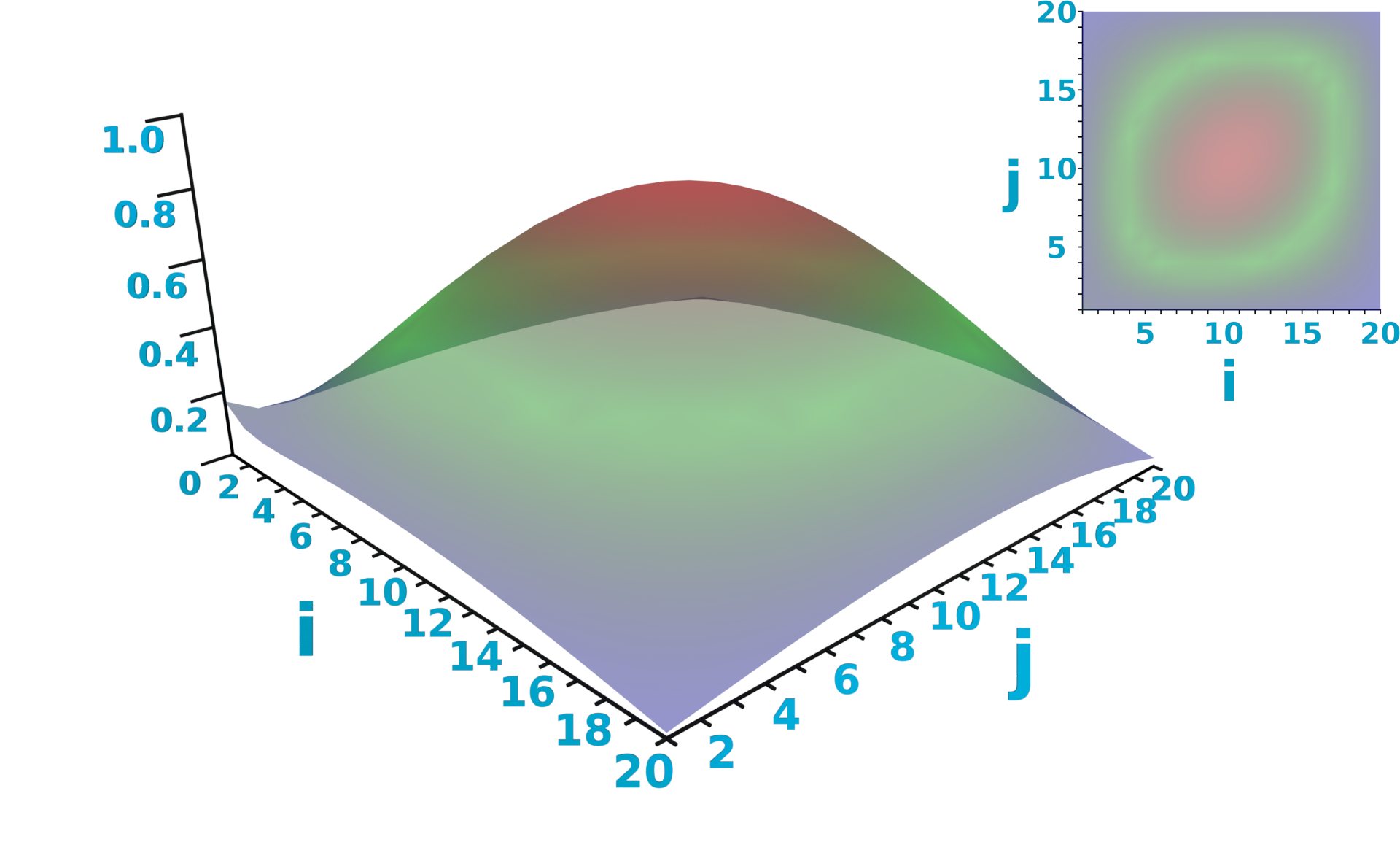
(a)

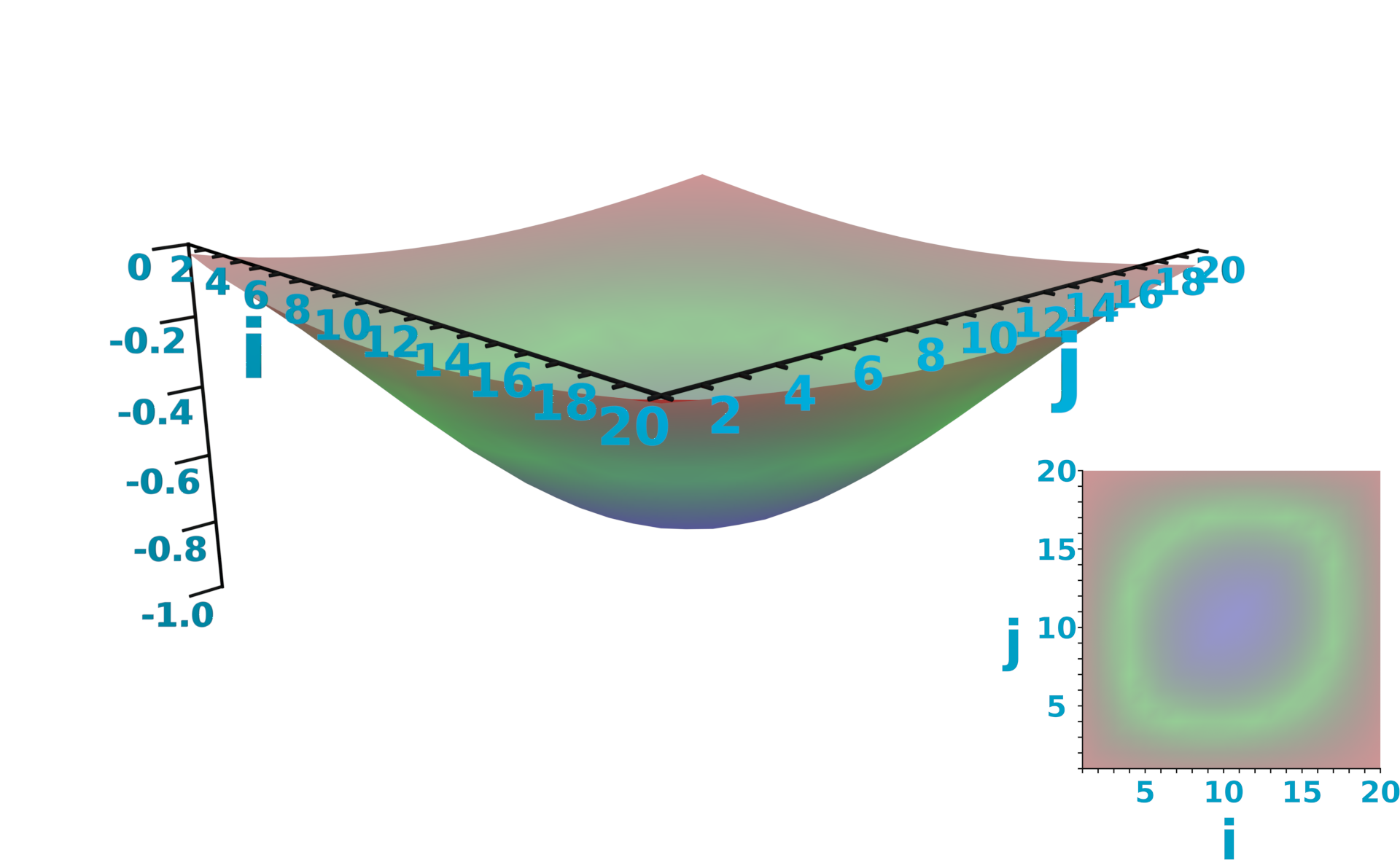
(b)

Figure 7: Normal and anomalous spin densities for a system with high anisotropy, $K/J=$5\text{\times}{10}^{-2}$$. All other parameters are equal to those in Fig. 6. LABEL:sub@fig:rholesser2a: normal density $\big{<}b^{\dagger}_{i}(t)b_{j}(t)\big{>}$. LABEL:sub@fig:rholesser2b: anomalous density $\big{<}b^{\dagger}_{i}(t)b^{\dagger}_{j}(t)\big{>}$.

At much greater anisotropy—$K/J=$5\text{\times}{10}^{-2}$$ shown in Fig 7—the amplitude of the spin density at the center of the sample increases significantly (Fig 7a), but the qualitative appearance of the profile remains broadly the same. However, as shown in Fig. 7b, the anomalous correlations now take a large negative value, highlighting that the Holstein-Primakoff magnons are no longer good basis states in the ferromagnetic bulk.

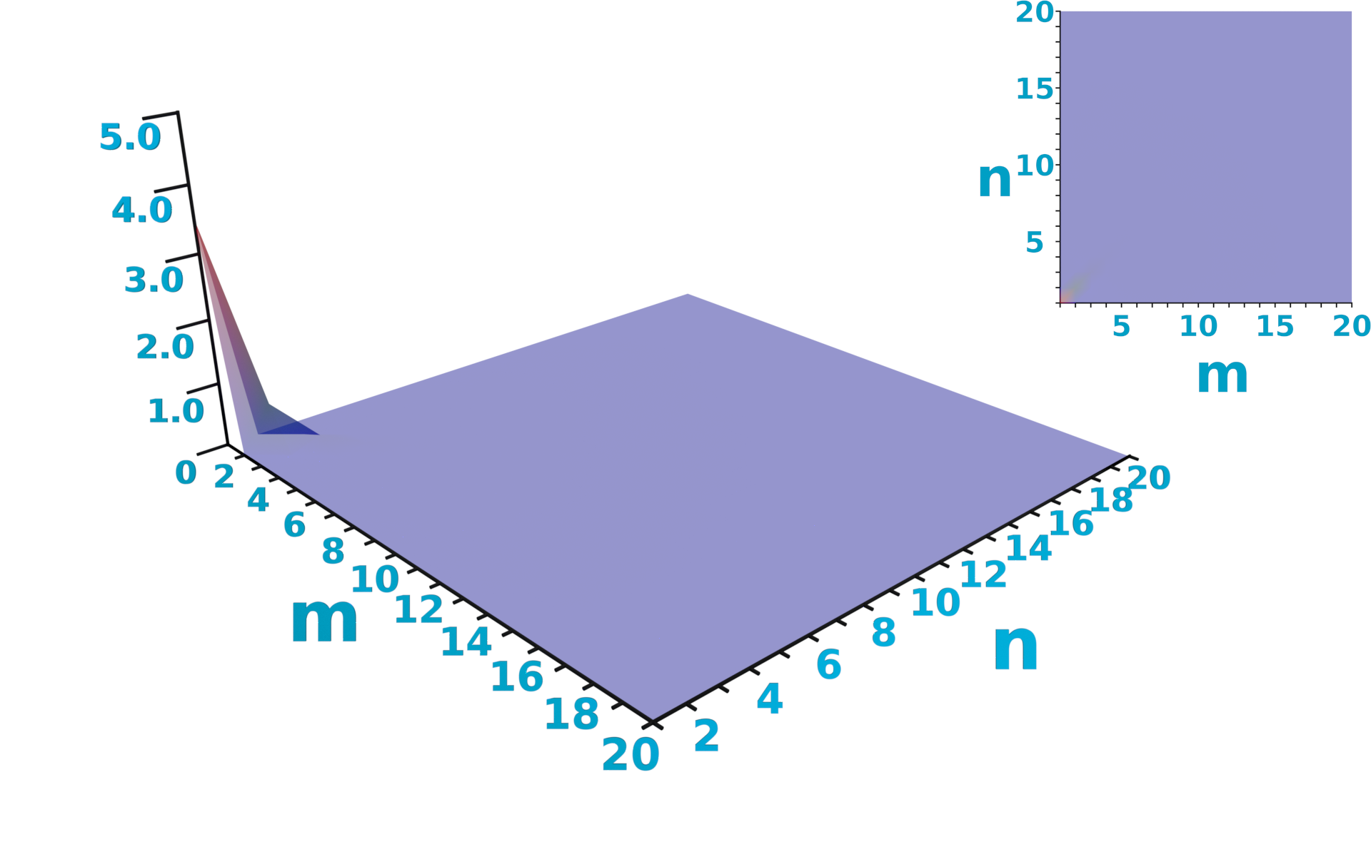
(a)

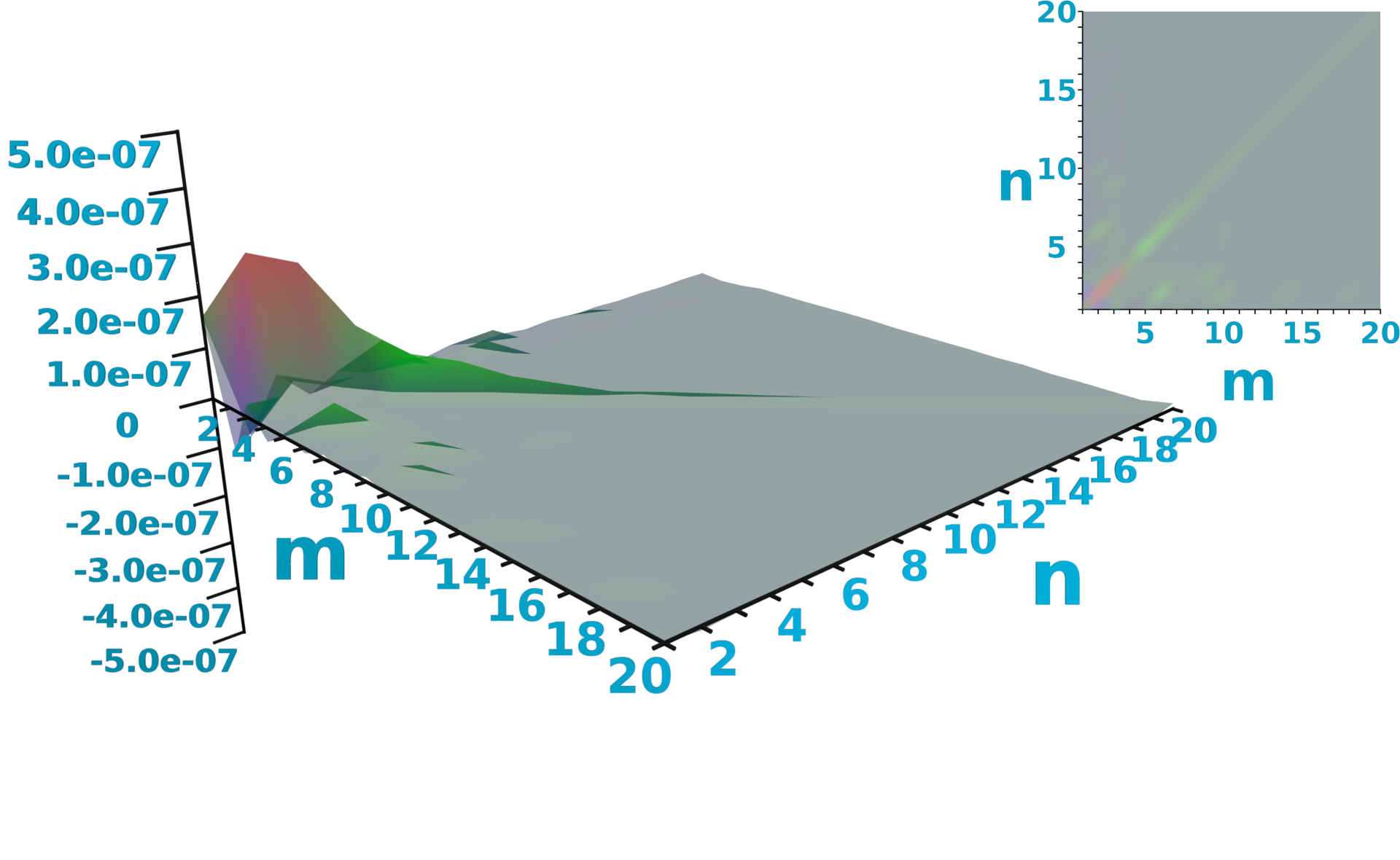
(b)

Figure 8: Normal and anomalous elliptical magnon densities for a system with low anisotropy, $K/J=$1\text{\times}{10}^{-7}$$. All other parameters are equal to those in Fig. 6. The horizontal axes represent the quantum numbers $m$ and $n$. LABEL:sub@fig:rholesser3a: normal density $\big{<}\psi^{\dagger}_{m}(t)\psi_{n}(t)\big{>}$. LABEL:sub@fig:rholesser3b: anomalous density $\big{<}\psi^{\dagger}_{m}(t)\psi^{\dagger}_{n}(t)\big{>}$. The minor (light green) fluctuations are near the scale of numerical error ($10^{-8}$) and may be unphysical.

In Figs. 8 and 9 we plot the equivalent matrices in the basis of elliptical magnons: the horizontal axes now represent the quantum number, and the diagonals of the plots are ordered by increasing energy. In this basis, the ordinary block $\big{<}\psi^{\dagger}_{m}\psi_{n}\big{>}$ of the correlation function $\big{<}\Psi^{\dagger}_{m}\Psi_{n}\big{>}$ is almost exactly diagonal at low anisotropy ($K/J=$1\text{\times}{10}^{-7}$$ shown in Fig. 8a). As we keep the gap $\varepsilon_{1}$ fixed, our chosen parameters lead to excitation of the lowest few modes only, regardless of anisotropy, with the overwhelming majority of quasiparticles being in the ground state (as indicated by the large spike at $m=n=1$). In Fig. 8b, it can be seen that the anomalous block $\big{<}\psi^{\dagger}_{m}\psi^{\dagger}_{n}\big{>}$ nearly vanishes, as expected (the same is true for $\big{<}\psi_{m}\psi_{n}\big{>}$).

(a)

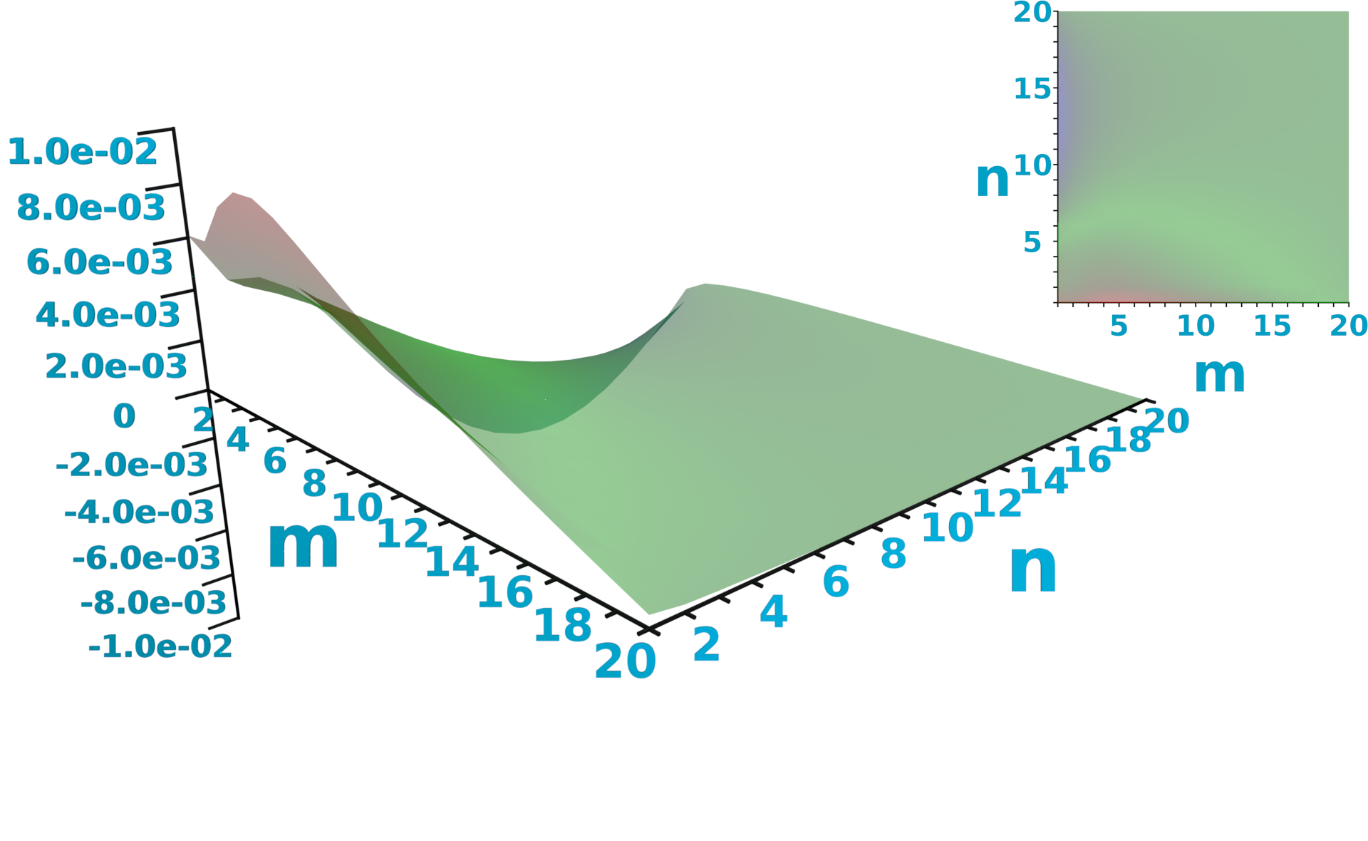
(b)

Figure 9: Normal and anomalous elliptical magnon densities for a system with high anisotropy, $K/J=$5\text{\times}{10}^{-2}$$. All other parameters are equal to those in Fig. 6. LABEL:sub@fig:rholesser4a: normal density $\big{<}\psi^{\dagger}_{m}(t)\psi_{n}(t)\big{>}$. LABEL:sub@fig:rholesser4b: anomalous density $\big{<}\psi^{\dagger}_{m}(t)\psi^{\dagger}_{n}(t)\big{>}$.

Figure 9a) shows that the qualitative behavior of the ordinary correlations $\big{<}\psi^{\dagger}_{m}\psi_{n}\big{>}$ does not change significantly even at the high anisotropy value $K/J=$5\text{\times}{10}^{-2}$$. However, the anomalous block $\big{<}\psi^{\dagger}_{m}\psi^{\dagger}_{n}\big{>}$, shown in Fig. 9b now exhibits a small but noticeable deviation from zero, and becomes asymmetric. This asymmetry ultimately stems from the fact that $\big{<}b^{\dagger}_{i}b_{j}\big{>}\neq\big{<}b_{i}b^{\dagger}_{j}\big{>}$. The bosonic relations are nevertheless preserved because the full matrix $\big{<}\Psi^{\dagger}_{m}\Psi_{n}\big{>}$ is symmetric.

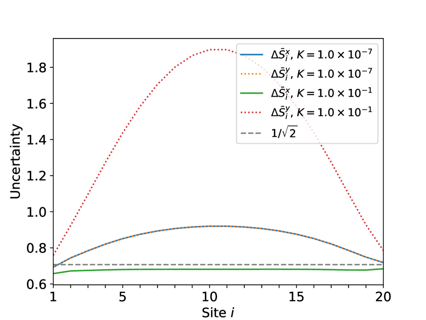
(a)

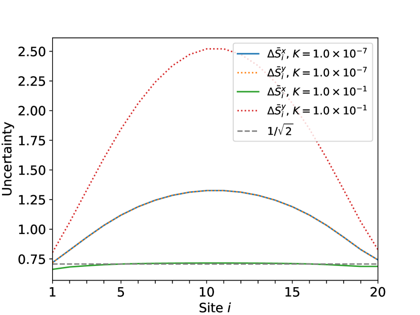
(b)

Figure 10: Uncertainty in the spin operators $S^{x}$ (solid lines) and $S^{y}$ (dotted lines), for a system of size $N=20$ with only the left lead attached ($\eta^{\mathrm{L}}=0.1$, $\eta^{\mathrm{R}}=0$), low Gilbert-like damping $\alpha=$1\text{\times}{10}^{-3}$$, temperature $k_{\mathrm{B}}T/J=0.1$, gap $\varepsilon_{1}/J=0.025$, and different anisotropies. When the spin uncertainty drops below $\frac{1}{\sqrt{2}}$ (dashed line), the state is squeezed. At very high anisotropy, the magnons become squeezed throughout the system. Note that the $\Delta\bar{S}^{x}$ and $\Delta\bar{S}^{y}$ curves lie on top of each other at $K/J=$1\text{\times}{10}^{-7}$$, indicating the magnons are coherent at low anisotropy. LABEL:sub@fig:squeeze-nobias: without applied bias ($\mu^{\mathrm{L}}=0$). LABEL:sub@fig:squeeze-bias: with bias at left lead ($\mu^{\mathrm{L}}/J=0.1$).

As explained previously, we may use the density matrix to directly compute uncertainty of the spin operators, which we expect to become squeezed at high anisotropy. In Fig. 10, we plot the uncertainty amplitudes $\Delta\bar{S}^{x}_{i}$ and $\Delta\bar{S}^{y}_{i}$ for $K/J=$1\text{\times}{10}^{-7}$$ and $K/J=$1\text{\times}{10}^{-1}$$, with weak left-lead coupling $\eta^{\mathrm{L}}=0.1$ and no right lead attached. In the case of zero bias ($\mu^{\mathrm{L}}=0$, Fig. 10a), it can be seen that high anisotropy causes the magnons to become squeezed throughout the sample. At site 1, where the left lead is attached, both $\Delta\bar{S}^{x}$ and $\Delta\bar{S}^{y}$ are squeezed, in an apparent violation of the uncertainty principle. However, this may be explained by the fact that we only consider the lowest-order self-energy contribution of the lead coupling: this ignores higher-order electronic contributions to the total wavefunction at the interface, and it stands to reason—although it remains to be verified—that the uncertainty principle is not violated if higher-order contributions are taken into account.

Taking only sites $i>1$ into account, we find that squeezing commences at site 20 (the ‘far side’ of the chain, where no lead is attached) for $K/J\approx$3\text{\times}{10}^{-2}$$. Squeezing increases with increasing anisotropy, with the effect being strongest at the center of the sample, where the overall spin density is the highest. By applying a spin bias at the attached lead ($\mu^{\mathrm{L}}/J=0.1$ shown in Fig. 10b), squeezing is diminished throughout the sample, and the overall uncertainty markedly increases. A local bias may thus be used to effect a global change in the uncertainty.

IV Conclusions and outlook

We have developed and numerically implemented a NEGF formalism to describe the transport of elliptically polarized magnons in finite-sized ferromagnetic insulators terminated by metallic leads. The presence of anisotropy in a ferromagnetic insulator can give rise to a novel parasitic local spin resistance, and additionally acts to suppress the spin conductance measured between the metallic leads. However, our model predicts that these effects are mild in ferromagnets with weak anisotropy, and become significant only when the ferromagnet exhibits strong anisotropy.

We have shown that the NEGF formalism allows theoretical access to the anomalous correlation functions $\big{<}b_{i}b_{j}\big{>}$ and $\big{<}b^{\dagger}_{i}b^{\dagger}_{j}\big{>}$, which may obtain a large amplitude in the presence of anisotropy, and provide a measure for the degree of nonconservation of spin and ellipticity of magnons. Likewise, the correlation functions $\big{<}\psi_{m}\psi_{n}\big{>}$ and $\big{<}\psi^{\dagger}_{m}\psi^{\dagger}_{n}\big{>}$ in the basis of eigenstates of the free anisotropic ferromagnetic insulator obtain a nonzero value in the presence of coupling to metallic leads which inject a well-defined amount of spin, provided the anisotropy is large and the lead coupling is sufficiently strong. Moreover, strong anisotropy produces squeezing of $\Delta\bar{S}^{x}$, which may be observable in the form of reduced shot noise [25] and find applications in quantum information science.

Although we have focussed on ferromagnets, where anisotropy tends to be significantly weaker than the exchange interaction, it stands to reason that much stronger observable effects may be realized in antiferromagnets, where similar anomalous Hamiltonian terms are introduced by coupling between sublattices, but are now governed by the exchange interaction itself [20].

While we have provided some examples of effects produced by the introduction of anisotropy, our model is simplistic, and omits several features one would expect to find in a realistic system. A possible extension, for example, would be the introduction of disorder, which can take the form of spatial fluctuations in both $\Delta$ and $K$. Moreover, our model considers only weak interactions between magnons and the leads and lattice (i.e. lowest-order self-energy terms), while higher-order contributions may be relevant to physical systems. We have likewise neglected magnon-magnon interactions, while several real systems are known or believed to violate this assumption [50, 51, 52].

Finally, the parameter space of our model (with or without extensions) is quite large, and therefore remains mostly unexplored. Hence, it is plausible that more observable effects of the spin-conservation breaking anisotropies can be found, for example through the spin Seebeck effect.

V Acknowledgements

R.A.D. is member of the D-ITP consortium, a program of the Dutch Organisation for Scientific Research (NWO) that is funded by the Dutch Ministry of Education, Culture and Science (OCW). This project has received funding from the European Research Council (ERC) under the European Union’s Horizon 2020 research and innovation programme (grant agreement No. 725509).

A.R. acknowledges financial support by the Deutsche Forschungsgemeinschaft (DFG) through Project No. KO/1442/10-1.

B.Z.R. acknowledges support by Iran Science Elites Federation (ISEF).

Appendix A Derivation of the steady-state spin current

We define the total spin current as the negative time-derivative of the total HP magnon number density (as each magnon carries spin 1), i.e.

$$j_{\mathrm{s}}^{\mathrm{tot}} =-\partial_{t}\operatorname{Tr}\left<b^{\dagger}(t)b(t)\right>$$

$$=-\frac{1}{2}\partial_{t}\left[\operatorname{Tr}\left\{\left<b^{\dagger}(t)b(t)\right>+\left<b(t)b^{\dagger}(t)\right>\right\}-N\right]$$

$$=-\frac{1}{2}\partial_{t}\operatorname{Tr}\left<\phi^{\dagger}(t)\phi(t)\right>=-\operatorname{Re}\operatorname{Tr}\left<\phi^{\dagger}(t)\partial_{t}\phi(t)\right>.$$ (43)

Note that the trace on the first two lines is over the spatial indices alone and therefore has $N$ terms, whereas on the last line, it is over the full matrix and therefore has $2N$ terms. To evaluate Eq. (43), we introduce a stochastic field

$$\xi(\omega) =-g(\omega)\phi(\omega)$$ (44)

obeying

$$\left<\xi(\omega)\xi^{\dagger}(\omega^{\prime})\right> =\uppi\mathrm{i}\delta(\omega-\omega^{\prime})\Sigma^{\mathrm{K}}(\omega).$$ (45)

By construction, $\xi$ is the Hubbard-Stratonovich field that decouples the quantum-quantum term of the Schwinger-Keldysh action for the continuum-limit field theory. A more detailed derivation is given e.g. by Kamenev [53].

Inserting Eq. (22) into Eq. (44) and taking the Fourier transform, we find the evolution equation

$$-\mathrm{i}\partial_{t}\phi(t) =\sigma_{3}h\phi(t)+\sigma_{3}\int\mathrm{d}t^{\prime}\Sigma(t-t^{\prime})\phi(t^{\prime})-\sigma_{3}\xi(t),$$ (46)

which we may plug into Eq. (43) to obtain

$$j_{\mathrm{s}}^{\mathrm{tot}} =-\operatorname{Im}\operatorname{Tr}\Bigg{\{}\left<\phi^{\dagger}(t)\sigma_{3}h\phi(t)\right>$$

$$\hskip 60.00009pt+\left<\phi^{\dagger}(t)\sigma_{3}\int\mathrm{d}t^{\prime}\Sigma(t-t^{\prime})\phi(t^{\prime})\right>$$

$$\hskip 60.00009pt-\left<\phi^{\dagger}(t)\sigma_{3}\xi(t)\right>\Bigg{\}}.$$ (47)

Here the first term is the Hamiltonian evolution of the system, and the second and third terms represent driving by external factors: the second term concerns the interaction with the lead electrons and with the field(s) responsible for Gilbert-like damping, and the third term contains the effect of quantum noise.

In the steady state, the total spin current vanishes by definition, and thus the first term necessarily cancels against the driving terms. In an experiment where the system is held out of equilibrium by external driving, the net external source/sink current are then given by the sum of the last two terms of Eq. (47). However, these terms, as given, sum over all of the spin currents within the system, including unobservable contributions that occur deep within the bulk and never exit the ferromagnet, whereas the actually observable spin currents are those which flow out of the leads. This quantity is obtained when one replaces $\Sigma$ with $\Sigma^{\mathrm{L/R}}$ and $\xi$ with $\xi^{\mathrm{L/R}}$ in Eq. (47). Here we define $\xi^{\mathrm{L/R}}$ to be the stochastic field obeying

$$\left<\xi^{\mathrm{L/R}}(\omega)\xi^{\dagger}(\omega^{\prime})\right> =2\uppi\mathrm{i}\delta(\omega-\omega^{\prime})\Sigma^{\mathrm{L/R}}(\omega)F^{\mathrm{L/R}}(\omega),$$ (48)

where $2\Sigma^{\mathrm{L/R}}(\omega)F^{\mathrm{L/R}}(\omega)$ is the left/right lead term of the Keldysh self energy.

Thus, focussing now on the spin current flowing out of the left lead (in the following derivation, one may obtain equivalent expressions for the right lead by swapping L and R), we find

$$j^{\mathrm{L,tot}}_{\mathrm{s}} =-\operatorname{Im}\operatorname{Tr}\Bigg{\{}\left<\phi^{\dagger}(t)\sigma_{3}\int\mathrm{d}t^{\prime}\Sigma^{\mathrm{L}}(t-t^{\prime})\phi(t^{\prime})\right>$$

$$\hskip 60.00009pt-\left<\phi^{\dagger}(t)\sigma_{3}\xi^{\mathrm{L}}(t)\right>\Bigg{\}}.$$ (49)

Next, by Fourier transforming and using Eq. (44) to write $$\phi \xi$$ in terms of , we obtain

$$j^{\mathrm{L,tot}}_{\mathrm{s}} =-\operatorname{Im}\operatorname{Tr}\int\frac{\mathrm{d}\omega}{2\uppi}\frac{\mathrm{d}\omega^{\prime}}{2\uppi}\mathrm{e}^{\mathrm{i}t(\omega^{\prime}-\omega)}$$

$$\hskip 60.00009pt\times\Bigg{\{}\left<\xi^{\dagger}(\omega)g^{\dagger}(\omega)\sigma_{3}\Sigma^{\mathrm{L}}(\omega^{\prime})g(\omega^{\prime})\xi(\omega^{\prime})\right>$$

$$\hskip 60.00009pt+\left<\xi^{\dagger}(\omega)g^{\dagger}(\omega)\sigma_{3}\xi^{\mathrm{L}}(\omega^{\prime})\right>\Bigg{\}}.$$ (50)

Reordering terms using the properties of the trace and making use of Eqs. (45), (48) and (27), this gives

$$j^{\mathrm{L,tot}}_{\mathrm{s}} =-\operatorname{Re}\operatorname{Tr}\int\frac{\mathrm{d}\omega}{2\uppi}\,g^{\dagger}(\omega)\sigma_{3}\Sigma^{\mathrm{L}}(\omega)g(\omega)$$

$$\hskip 60.00009pt\times\Bigg{\{}\Sigma^{\mathrm{L}}(\omega)F^{\mathrm{L}}(\omega)+\Sigma^{\mathrm{R}}(\omega)F^{\mathrm{R}}(\omega)$$

$$\hskip 60.00009pt+\Sigma^{\mathrm{B}}(\omega)\mathcal{T}^{-1}F^{\mathrm{B}}(\omega)\mathcal{T}+g^{-1}(\omega)F^{\mathrm{L}}(\omega)\Bigg{\}}.$$ (51)

Inserting the Dyson equation for $$g^{-1}(\omega)$$, we find

$$j^{\mathrm{L,tot}}_{\mathrm{s}} =-\operatorname{Re}\operatorname{Tr}\int\frac{\mathrm{d}\omega}{2\uppi}\Bigg{\{}\iota^{\mathrm{R\to L}}(\omega)+\iota^{\mathrm{B\to L}}(\omega)$$

$$\hskip 60.00009pt+g^{\dagger}(\omega)\sigma_{3}\Sigma^{\mathrm{L}}(\omega)g(\omega)\left[\omega\sigma_{3}-h\right]F^{\mathrm{L}}(\omega)\Bigg{\}},$$ (52)

where $\iota^{\mathrm{R\to L}}(\omega)$ and $\iota^{\mathrm{B\to L}}$ are given by Eqs. (38) and (38b), respectively. By using that $\operatorname{Re}\operatorname{Tr}M=\frac{1}{2}\operatorname{Tr}(M+M^{\dagger})$ for an arbitrary square matrix $M$, the term involving $\omega\sigma_{3}$ can easily be shown to vanish. In a similar vein, we find

$$-\operatorname{Re}\operatorname{Tr} \left\{g^{\dagger}(\omega)\sigma_{3}\Sigma^{\mathrm{L}}(\omega)g(\omega)hF^{\mathrm{L}}(\omega)\right\}$$

$$\quad=\frac{1}{2}\operatorname{Tr}\left\{g^{\dagger}(\omega)\sigma_{3}\Sigma^{\mathrm{L}}(\omega)g(\omega)\left[F^{\mathrm{L}}(\omega),h\right]\right\}.$$ (53)

In the absence of a spin accumulation, $F^{\mathrm{L}}(\omega)$ becomes a scalar function multiplying the identity matrix, causing the commutator to vanish. Therefore, we may add the term

$$0 =\operatorname{Tr}g^{\dagger}(\omega)\sigma_{3}\Sigma^{\mathrm{L}}(\omega)g(\omega)h\left.F^{\mathrm{L}}(\omega)\right|_{\mu^{\mathrm{L}}=0},$$ (54)

thereby recovering Eq. 38). Finally, in the limit $K\to 0$, the Hamiltonian $h$ becomes block-diagonal, so that the commutator in Eq. (53) causes $\iota^{\mathrm{L}}(\omega)$ to vanish in absence of anisotropy.

References

- Zhang et al. [2014] Y. Zhang, W. Zhao, J.-O. Klein, W. Kang, D. Querlioz, Y. Zhang, D. Ravelosona, and C. Chappert, Spintronics for low-power computing, in 2014 Design, Automation & Test in Europe Conference & Exhibition (DATE) (IEEE, 2014) pp. 1–6.
- Pinna et al. [2018] D. Pinna, F. Abreu Araujo, J. V. Kim, V. Cros, D. Querlioz, P. Bessiere, J. Droulez, and J. Grollier, Skyrmion Gas Manipulation for Probabilistic Computing, Physical Review Applied 9, 064018 (2018), arXiv:1701.07750 [cond-mat.mes-hall] .
- Song et al. [2020] K. M. Song, J.-S. Jeong, B. Pan, X. Zhang, J. Xia, S. Cha, T.-E. Park, K. Kim, S. Finizio, J. Raabe, et al., Skyrmion-based artificial synapses for neuromorphic computing, Nature Electronics 3, 148 (2020).
- Parkin et al. [2008] S. S. P. Parkin, M. Hayashi, and L. Thomas, Magnetic Domain-Wall Racetrack Memory, Science 320, 190 (2008).
- Vélez et al. [2019] S. Vélez, J. Schaab, M. S. Wörnle, M. Müller, E. Gradauskaite, P. Welter, C. Gutgsell, C. Nistor, C. L. Degen, M. Trassin, M. Fiebig, and P. Gambardella, High-speed domain wall racetracks in a magnetic insulator, Nature Communications 10, 4750 (2019), arXiv:1902.05639 [physics.app-ph] .
- Kruglyak et al. [2010] V. V. Kruglyak, S. O. Demokritov, and D. Grundler, Magnonics, Journal of Physics D Applied Physics 43, 264001 (2010).
- Cornelissen et al. [2015] L. J. Cornelissen, J. Liu, R. A. Duine, J. B. Youssef, and B. J. van Wees, Long-distance transport of magnon spin information in a magnetic insulator at room temperature, Nature Physics 11, 1022 (2015), arXiv:1505.06325 [cond-mat.mes-hall] .
- Fan et al. [2020] Y. Fan, P. Quarterman, J. Finley, J. Han, P. Zhang, J. T. Hou, M. D. Stiles, A. J. Grutter, and L. Liu, Manipulation of coupling and magnon transport in magnetic metal-insulator hybrid structures, Phys. Rev. Applied 13, 061002 (2020), arXiv:2002.08266 [cond-mat.mtrl-sci] .
- Wu et al. [2018] H. Wu, L. Huang, C. Fang, B. S. Yang, C. H. Wan, G. Q. Yu, J. F. Feng, H. X. Wei, and X. F. Han, Magnon Valve Effect between Two Magnetic Insulators, Physical Review Letters 120, 097205 (2018), arXiv:1801.06617 [cond-mat.mes-hall] .
- Guo et al. [2020] C. Guo, C. Wan, W. He, M. Zhao, Z. Yan, Y. Xing, X. Wang, P. Tang, Y. Liu, S. Zhang, et al., A nonlocal spin hall magnetoresistance in a platinum layer deposited on a magnon junction, Nature Electronics , 1 (2020).
- Prasai et al. [2017] N. Prasai, B. A. Trump, G. G. Marcus, A. Akopyan, S. X. Huang, T. M. McQueen, and J. L. Cohn, Ballistic magnon heat conduction and possible Poiseuille flow in the helimagnetic insulator Cu2OSeO3, Physical Review B 95, 224407 (2017), arXiv:1705.06328 [cond-mat.str-el] .
- Oyanagi et al. [2020] K. Oyanagi, T. Kikkawa, and E. Saitoh, Magnetic field dependence of the nonlocal spin Seebeck effect in Pt/YIG/Pt systems at low temperatures, AIP Advances 10, 015031 (2020), arXiv:1910.04046 [cond-mat.mtrl-sci] .
- Cornelissen et al. [2016] L. J. Cornelissen, K. J. H. Peters, G. E. W. Bauer, R. A. Duine, and B. J. van Wees, Magnon spin transport driven by the magnon chemical potential in a magnetic insulator, Physical Review B 94, 014412 (2016), arXiv:1604.03706 [cond-mat.mes-hall] .
- Zheng et al. [2017] J. Zheng, S. Bender, J. Armaitis, R. E. Troncoso, and R. A. Duine, Green’s function formalism for spin transport in metal-insulator-metal heterostructures, Physical Review B 96, 174422 (2017), arXiv:1709.03775 [cond-mat.mes-hall] .
- Nakata et al. [2017] K. Nakata, P. Simon, and D. Loss, Spin currents and magnon dynamics in insulating magnets, Journal of Physics D: Applied Physics 50, 114004 (2017).
- Ulloa et al. [2019] C. Ulloa, A. Tomadin, J. Shan, M. Polini, B. J. van Wees, and R. A. Duine, Non-local spin transport as a probe of viscous magnon fluids, arXiv e-prints (2019), arXiv:1903.02790 [cond-mat.mes-hall] .
- Holstein and Primakoff [1940] T. Holstein and H. Primakoff, Field Dependence of the Intrinsic Domain Magnetization of a Ferromagnet, Physical Review 58, 1098 (1940).
- Heisenberg [1928] W. Heisenberg, Zur Theorie des Ferromagnetismus, Zeitschrift fur Physik 49, 619 (1928).
- Bender et al. [2012] S. A. Bender, R. A. Duine, and Y. Tserkovnyak, Electronic Pumping of Quasiequilibrium Bose-Einstein-Condensed Magnons, Physical Review Letters 108, 246601 (2012), arXiv:1111.2382 [cond-mat.mes-hall] .
- Kamra et al. [2020] A. Kamra, W. Belzig, and A. Brataas, Magnon-squeezing as a niche of quantum magnonics, Applied Physics Letters 117, 090501 (2020), arXiv:2008.13536 [cond-mat.mtrl-sci] .
- Zheng et al. [2020] J. Zheng, A. Rückriegel, S. A. Bender, and R. A. Duine, Ellipticity and dissipation effects in magnon spin valves, Physical Review B 101, 094402 (2020), arXiv:1911.12017 [cond-mat.mes-hall] .
- Ulloa and Duine [2018] C. Ulloa and R. A. Duine, Magnon Spin Hall Magnetoresistance of a Gapped Quantum Paramagnet, Physical Review Letters 120, 177202 (2018), arXiv:1710.04431 [cond-mat.mes-hall] .
- Keldysh et al. [1965] L. V. Keldysh et al., Diagram technique for nonequilibrium processes, Sov. Phys. JETP 20, 1018 (1965).
- Rammer [2007] J. Rammer, Quantum field theory of non-equilibrium states (Cambridge Univ. Press, Cambridge, 2007).
- Kamra and Belzig [2016] A. Kamra and W. Belzig, Super-Poissonian Shot Noise of Squeezed-Magnon Mediated Spin Transport, Physical Review Letters 116, 146601 (2016), arXiv:1602.07513 [cond-mat.mes-hall] .
- Walls [1983] D. F. Walls, Squeezed states of light, Nature 306, 141 (1983).
- Aggarwal et al. [2020] N. Aggarwal, T. J. Cullen, J. Cripe, G. D. Cole, R. Lanza, A. Libson, D. Follman, P. Heu, T. Corbitt, and N. Mavalvala, Room-temperature optomechanical squeezing, Nature Physics 16, 784 (2020).
- Doornenbal et al. [2019] R. J. Doornenbal, A. Roldán-Molina, A. S. Nunez, and R. A. Duine, Spin-Wave Amplification and Lasing Driven by Inhomogeneous Spin-Transfer Torques, Physical Review Letters 122, 037203 (2019).
- Rückriegel and Duine [2020] A. Rückriegel and R. A. Duine, Hannay angles in magnetic dynamics, Annals of Physics 412, 168010 (2020), arXiv:1910.05099 [cond-mat.mes-hall] .
- Graß et al. [2011] T. D. Graß, F. E. A. dos Santos, and A. Pelster, Excitation spectra of bosons in optical lattices from the Schwinger-Keldysh calculation, Physical Review A 84, 013613 (2011), arXiv:1011.5639 [cond-mat.quant-gas] .
- Colpa [1978] J. H. P. Colpa, Diagonalization of the quadratic boson hamiltonian, Physica A Statistical Mechanics and its Applications 93, 327 (1978).
- Note [1] Specifically, the components of the paravector with quantum number corresponding to site are simply , up to paranormalization.
- Datta [2000] S. Datta, Nanoscale device modeling: the green’s function method, Superlattices and microstructures 28, 253 (2000).
- Ganzhorn et al. [2016] K. Ganzhorn, S. Klingler, T. Wimmer, S. Geprägs, R. Gross, H. Huebl, and S. T. B. Goennenwein, Magnon-based logic in a multi-terminal YIG/Pt nanostructure, Applied Physics Letters 109, 022405 (2016), arXiv:1604.07262 [cond-mat.mes-hall] .
- Note [2] Thus the full matrix has nonzero components at indices and .
- Gilbert [2004] T. L. Gilbert, A Phenomenological Theory of Damping in Ferromagnetic Materials, IEEE Transactions on Magnetics 40, 3443 (2004).
- Haug [2008] H. Haug, Quantum kinetics in transport and optics of semiconductors (Springer, Berlin New York, 2008).
- Robertson [1929] H. P. Robertson, The Uncertainty Principle, Physical Review 34, 163 (1929).
- Ventra [2008] M. Ventra, Electrical transport in nanoscale systems (Cambridge University Press, Cambridge, UK New York, 2008).
- Kennelly [1899] A. E. Kennelly, The equivalence of triangles and three-pointed stars in conducting networks, Electrical world and engineer 34, 413 (1899).
- Bauer et al. [2012] G. E. W. Bauer, E. Saitoh, and B. J. van Wees, Spin caloritronics, Nature Materials 11, 391 (2012), arXiv:1107.4395 [cond-mat.mes-hall] .
- Sharko et al. [2020] S. A. Sharko, A. I. Serokurova, N. N. Novitskii, V. A. Ketsko, M. N. Smirnova, R. Gieniusz, A. Maziewski, and A. I. Stognij, Ferromagnetic and FMR properties of the YIG/TiO2/PZT structures obtained by ion-beam sputtering, Journal of Magnetism and Magnetic Materials 514, 167099 (2020).
- Xie et al. [2017] L.-S. Xie, G.-X. Jin, L. He, G. E. W. Bauer, J. Barker, and K. Xia, First-principles study of exchange interactions of yttrium iron garnet, Physical Review B 95, 014423 (2017), arXiv:1701.00110 [cond-mat.mtrl-sci] .
- Edmonds and Petersen [1959] D. Edmonds and R. Petersen, Effective exchange constant in yttrium iron garnet, Physical Review Letters 2, 499 (1959).
- Cherepanov et al. [1993] V. Cherepanov, I. Kolokolov, and V. L’vov, The saga of YIG: Spectra, thermodynamics, interaction and relaxation of magnons in a complex magnet, Physics Reports 229, 81 (1993).
- Princep et al. [2017] A. J. Princep, R. A. Ewings, S. Ward, S. Tóth, C. Dubs, D. Prabhakaran, and A. T. Boothroyd, The full magnon spectrum of yttrium iron garnet, npj Quantum Materials 2, 63 (2017), arXiv:1705.06594 [cond-mat.str-el] .
- Coey [2009] J. M. D. Coey, Magnetism and magnetic materials (Cambridge University Press, Cambridge New York, 2009).
- Poimanov et al. [2020] V. D. Poimanov, A. N. Kuchko, and V. V. Kruglyak, Scattering of exchange spin waves from a helimagnetic layer sandwiched between two semi-infinite ferromagnetic media, Physical Review B 102, 104414 (2020).
- Kaplan and Kaplan [2014] B. Kaplan and R. Kaplan, Anisotropy effects on the spin wave gap of two dimensional magnets at zero temperature, Journal of Magnetism and Magnetic Materials 356, 95 (2014).
- Gros et al. [1997] C. Gros, W. Wenzel, A. Fledderjohann, P. Lemmens, M. Fischer, G. Güntherodt, M. Weiden, C. Geibel, and F. Steglich, Magnon-magnon interactions in the spin-peierls compound , Phys. Rev. B 55, 15048 (1997), arXiv:cond-mat/9612101 [cond-mat.str-el] .
- Chen et al. [2018] J. Chen, C. Liu, T. Liu, Y. Xiao, K. Xia, G. E. W. Bauer, M. Wu, and H. Yu, Strong Interlayer Magnon-Magnon Coupling in Magnetic Metal-Insulator Hybrid Nanostructures, Physical Review Letters 120, 217202 (2018).
- Xiong et al. [2020] Y. Xiong, Y. Li, M. Hammami, R. Bidthanapally, J. Sklenar, X. Zhang, H. Qu, G. Srinivasan, J. Pearson, A. Hoffmann, V. Novosad, and W. Zhang, Probing magnon-magnon coupling in exchange coupled Y3Fe5O12/Permalloy bilayers with magneto-optical effects, Scientific Reports 10, 12548 (2020), arXiv:1912.13407 [cond-mat.mtrl-sci] .
- Kamenev [2002] A. Kamenev, Keldysh and doi-peliti techniques for out-of-equilibrium systems, in Strongly Correlated Fermions and Bosons in Low-Dimensional Disordered Systems (Springer, 2002) pp. 313–340.