Throttling Equilibria in Auction Markets

Abstract

Throttling is a popular method of budget management for online ad auctions in which the platform modulates the participation probability of an advertiser in order to smoothly spend her budget across many auctions. In this work, we investigate the setting in which all of the advertisers simultaneously employ throttling to manage their budgets, and we do so for both first-price and second-price auctions. We analyze the structural and computational properties of the resulting equilibria. For first-price auctions, we show that a unique equilibrium always exists, is well-behaved and can be computed efficiently via tâtonnement-style decentralized dynamics. In contrast, for second-price auctions, we prove that even though an equilibrium always exists, the problem of finding an equilibrium is PPAD-complete, there can be multiple equilibria, and it is NP-hard to find the revenue maximizing one. We also compare the equilibrium outcomes of throttling to those of multiplicative pacing, which is the other most popular and well-studied method of budget management. Finally, we characterize the Price of Anarchy of these equilibria for liquid welfare by showing that it is at most 2 for both first-price and second-price auctions, and demonstrating that our bound is tight.

1 Introduction

Online ad auctions are the workhorse of the internet advertising industry; when a user visits an internet-based platform, an auction is run among the interested advertisers to determine the ad to be displayed to the user. Due to the large volume of these auctions, many advertisers are budget constrained: if they are allowed to participate in all the auctions they are interested in, they would end up spending more than their budget. This motivates the platforms to offer budget-management services. The focus of this paper is a popular budget-management service known as throttling (or alternatively as probabilistic pacing) which is offered by internet giants like Facebook (Facebook-Guide, ), Google (Karande et al., 2013) and LinkedIn (Agarwal et al., 2014). Throttling manages the expenditure of an advertiser by controlling the probability with which she participates in each individual auction.

The use of participation probability as a control lever allows the platform to evenly spread out an advertiser’s expenditure throughout her advertising campaign, while ensuring that she does not spend more than her budget. Furthermore, in contrast to other budget-management methods like multiplicative pacing, throttling does not modify the bids of the advertisers to achieve this, which is essential for advertisers aiming to maintain a stable cost-per-opportunity (Facebook-Guide, ). Additionally, in practice, many advertisers do not opt into budget-management services that modify their bids, forcing the platform to satisfy their budget constraint by only controlling their participation probability, as in throttling (Karande et al., 2013). Importantly, throttling also gives advertisers a more representative sample of users for which they are eligible and their bid is competitive (Karande et al., 2013). This is in contrast to budget-management approaches that modify bids, such as multiplicative pacing, which biases the allocation towards users where the advertiser has a high probability of getting a click, relative to other advertisers. Many advertisers place a premium on the predictability and representative samples offered by unmodified bids, motivating the platforms to offer throttling as a budget-management option.

Throttling has received significant attention in previous work, the vast majority of which studies it from the perspective of a single buyer participating in repeated generalized second-price auctions (see Section 1.2). In contrast, the scenario where all of the buyers simultaneously employ throttling to manage their budgets, and the resulting system-level properties, have received very little attention. In this paper, we attempt to remedy this situation by providing a structural and computational analysis of simultaneous multi-buyer throttling for both first-price and second-price auctions. More specifically, we analyze the resulting games, with an emphasis on equilibria and repeated play.

1.1 Main Contributions

We define a throttling game with budget-constrained buyers (advertisers) and stochastic good types (user types), in which each buyer chooses the probability with which she participates in the auction, with the goal of maximizing her expected utility while satisfying her budget constraint in expectation. Repeated play of this throttling game captures the repeated online ad auction setting in which each buyer employs throttling to manage their budget. Furthermore, we define the concept of throttling equilibrium for this game, show its equivalence to pure strategy Nash equilibrium, and analyze it with an emphasis on its structural and computational properties. We summarize our results below.

First-price Auctions: We show that a throttling equilibrium always exists, and characterize it as the maximal element in the set of participation probabilities that result in all buyers satisfying their budgets (Theorem 5). Furthermore, we use this characterization to establish its uniqueness. On the computational front, we describe decentralized dynamics in which buyers repeatedly play the throttling game and make simple tâtonnement-style adjustments to their participation probabilities based on their expected expenditure (Algorithm 1). We show that these tâtonnement-style dynamics converge to an approximate throttling equilibrium in polynomial time (Theorem 7).

Second-price Auctions: We begin by establishing that a throttling equilibrium always exists for second-price auctions (Theorem 8), but find that it may not be unique, and for some games all throttling equilibria can be irrational. Next, we prove results about the computational complexity of finding throttling equilibria, which requires the use of terminology from computational complexity theory. Before summarizing those results, we make a note for readers who may not be familiar with complexity theory: In order to make our results more accessible, we provide an informal description of them at the head of every subsection, in an attempt to avoid letting complexity-theoretic terminology obscure the conclusions derived from the result. Continuing on with the summary of our results, we prove that the problem of computing approximate throttling equilibria is PPAD-hard even when each good has at most three bids (Theorem 9), by showing a reduction from the PPAD-hard problem of computing an approximate equilibrium of a threshold game (Papadimitriou and Peng, 2021). As a consequence, we show that, unlike first-price auctions, no dynamics can converge in polynomial time to a second-price throttling equilibrium (assuming PPAD-complete problems cannot be solved in polynomial time). Furthermore, we place the problem of computing approximate throttling equilibria in the class PPAD by showing a reduction to the problem of finding a Brouwer fixed point of a Lipschitz mapping from a unit hypercube to itself (Theorem 15); the latter is known to be in PPAD via Sperner’s lemma (e.g. see Chen et al. 2009). We provide additional evidence of the computational challenges that afflict throttling for second-price auctions by proving the NP-hardness of finding a revenue-maximizing approximate throttling equilibrium (Theorem 17). We complement these hardness results by describing a polynomial-time algorithm for computing throttling equilibria for the special case in which there are at most two bids on each good (Algorithm 2), thereby precisely delineating the boundary of tractability.

Comparing Pacing and Throttling: As mentioned earlier, multiplicative pacing is another popular method of budget management, where buyers shade their bids to smoothly spend their budgets. In contrast to throttling, equilibria and dynamics in settings where all of the buyers use pacing have received significant attention (Borgs et al., 2007; Balseiro and Gur, 2019; Conitzer et al., 2018, 2019; Chen et al., 2021). This allows us to compare two of the most popular methods of budget management (Balseiro and Gur, ). We show that, for first-price auctions, the revenue of the unique throttling equilibrium and the unique pacing equilibrium, although incomparable directly, are always within a factor of 2 of each other (Theorem 19). Moreover, we find that pacing and throttling equilibria share a remarkably similar computational and structural landscape, as summarized in Table 1 and Table 2. In view of this comparison, our work can be seen as providing the analogous set of results for throttling equilibria that Borgs et al. (2007); Conitzer et al. (2018, 2019); Chen et al. (2021) proved for pacing equilibria. Our results reaffirm what the analysis of pacing suggested: budget management for first-price auctions is more well-behaved as compared to second-price auctions.

Existence	Rationality	Multiplicity	Computational Complexity	Efficient Dynamics
Always	Not always	Always unique	Poly.-time for approx. eq.	For approx. eq.
Always	Always	Always unique	Poly.-time for exact eq.	For approx. eq.
(Conitzer et al., 2019)	(Conitzer et al., 2019)	(Conitzer et al., 2019)	(Conitzer et al., 2019)	(Borgs et al., 2007)

Table 1: Comparison of throttling (top row) and pacing equilibria (bottom row) for first-price auctions.

Existence	Rationality	Multiplicity	Computational Complexity	Revenue Max.
Always	Not always	Possibly infinite	PPAD-complete for approx. eq	NP-hard
Always	Always	Possible	PPAD-complete for both exact	NP-hard
(Conitzer et al., 2018)	(Chen et al., 2021)	(Conitzer et al., 2018)	and approx. eq. (Chen et al., 2021)	(Conitzer et al., 2018)

Table 2: Comparison of throttling equilibria (top row) and pacing equilibria (bottom row) for second-price auctions.

Price of Anarchy: Liquid welfare (Dobzinski and Leme, 2014; Azar et al., 2017) is a measure of efficiency for settings with budget constraints, like the one considered in this work. It corresponds to the maximum revenue (liquidity) that can be extracted with full knowledge of the buyers’ values/bids, and reduces to social welfare when the budgets are non-binding. We show that the liquid welfare under any throttling equilibrium is at most a factor of 2 away from the liquid welfare that can be obtained by a central planner with complete information of the buyers bids/values, i.e., the Price of Anarchy is at most 2. We do so for both first-price and second-price auctions. Moreover, we provide examples to show that this bound is tight for both auction formats.

1.2 Additional Related Work

Budget management in online ad auctions has received widespread attention in the literature. Here, we review the papers which most closely relate to ours. We begin by reviewing the work on throttling, then give a broad overview of the other models for bidding under budget constraints considered in the literature, and finally conclude with a discussion of the work on multiplicative pacing, which we use in our comparisons.

Among work on throttling, Balseiro et al. (2021) is the closest to ours, and acts as the inspiration for our model and terminology. In Balseiro et al. (2021), the authors study system equilibria under various budget management strategies in second-price auctions, one of them being throttling. They show that throttling satisfies desirable incentive properties, and, under the special case when buyer values are symmetric, they compare equilibrium seller revenue and total welfare for throttling to a variety of other budget management techniques. Crucially, unlike our work, Balseiro et al. (2021) lacks a computational analysis and focuses solely on second-price auctions. Throttling has also received significant attention in other lines of research. Agarwal et al. (2014) study throttling in generalized second-price (GSP) auctions from the perspective of a single buyer, provide an algorithm which determines the participation probability based on user traffic forecasts, and analyze its performance empirically on real data from LinkedIn. Similarly, Xu et al. (2015) provide and empirically evaluate practical algorithms for throttling on data from demand-side platforms. Karande et al. (2013) use throttling (under the name Vanilla Probabilistic Throttling) as the benchmark in the GSP auction setting to evaluate the budget management algorithm they describe on data from Google, and find that it empirically outperforms throttling on the metrics they study. Importantly, they do not engage in an equilibrium analysis, and their algorithm does not provide a representative sample of the traffic to advertisers.

There is also a significant body of work which proposes alternatives to pacing and throttling methods. Charles et al. (2013) study regret-free budget-smoothing policies in which the platform selects the random subset of buyers that participate in the GSP auction for each good. They show that such policies always exist, and, under the small-bids assumption, give an efficient algorithm for the special case of second-price auctions. There is also a significant body of work that models budget management in first-price auctions as an allocation problem under stochastic and adversarial input, starting with the work of Mehta et al. (2007). See Mehta (2013) for a survey. We emphasize that in this work, our goal is to study the budget-management mechanisms that are employed in practice, which is why we focus on comparing pacing and throttling.

Unlike throttling, equilibrium analysis for the setting where all buyers simultaneously use multiplicative pacing is well-understood. Conitzer et al. (2018) define and study pacing equilibria in second-price auctions. They show that it always exists and study its structural properties. Chen et al. (2021) recently analyzed the computational complexity of finding pacing equilibria in second-price auctions, and proved that the problem is PPAD-complete. For first-price auctions, Borgs et al. (2007) describe a simple tâtonnement-style dynamics and prove its efficient convergence to a pacing equilibrium. Conitzer et al. (2019) characterize the structural properties of pacing equilibria in first-price auctions and give a market-equilibrium based algorithm for computing it. A summary of these results can be found in the second row of Table 1 and Table 2.

Finally, Price of Anarchy for liquid welfare has been studied in a variety of settings with budget-constrained buyers. Azar et al. (2017) show that the Price of Anarchy of liquid welfare is 2 for simultaneous first-price and second-price auctions in the multi-item setting. For mixed-strategy Nash equilibria they showed an upper bound of 51.5, with both results requiring the “no over-budgeting” assumption that requires the sum of bids to be less than the budget. Their results cannot be compared to ours because we only require the budget constraints to be satisfied in expectation, and more generally the settings have different action sets (throttling parameters versus bids). Balseiro et al. (2022) study a contextual-value auction model with strategic agents and establish the existence of pacing-based equilibria for all standard auction formats, including first-price and second-price auctions as special cases. They go on to show that pacing equilibria have a Price of Anarchy of at most 2 for all standard auctions in their model. Gaitonde et al. (2022) study the repeated-auction setting and show that the Price of Anarchy is bounded above by 2 even if the system is not in equilibrium, provided that all of the buyers use a generalization of the dual-descent-based pacing algorithm introduced in Balseiro and Gur (2019).

2 Model

Consider a seller who has $m$ types of goods to sell, and $n$ budget constrained buyers who are interested in buying these goods. The seller runs an auction amongst the buyers in order to make the sale. We assume that the type of good to be sold is drawn from some known distribution $d=(d_{1},\dots,d_{m})$, i.e., the good to be sold is of type $j$ with probability $d_{j}$. Buyer $i$ bids $\tilde{b}_{ij}$ on good type $j$, for all $i\in[n],j\in[m]$, and has a per-auction budget of $B_{i}>0$. To control their budget expenditure, each buyer $i$ is associated with a throttling parameter $\theta_{i}\in[0,1]$, which represents the probability with which she participates in the auction: each buyer $i$ independently flips a biased coin which comes up heads with probability $\theta_{i}$, and submits their bid $\tilde{b}_{ij}$ if the coin comes up heads, while submitting no bid if the coin comes up tails.

We focus on the setting where each buyer wishes to satisfy her budget constraint in expectation, i.e., buyer $i$ would like to spend less than $B_{i}$ in expectation over the good types and participation coin flips of all buyers. Requiring the budget constraints to be satisfied in expectation draws its motivation from the large number of auctions that are run by online-advertising platforms, in conjunction with concentration arguments, and has been employed by previous works on budget management in online auctions (see, e.g., Gummadi et al. (2012); Abhishek and Hosanagar (2013); Balseiro et al. (2015, 2017); Balseiro and Gur (2019); Conitzer et al. (2018)). Additionally, in this paper, we restrict our attention to the two most commonly-used auction formats in online advertising: first-price auctions and second-price auctions. In a first-price auction, the participating buyer with the highest bid wins the good and pays her bid, whereas in a second-price auction, the participating buyer with the highest bid wins the good and pays the second-highest bid among the participating buyers. Our model can be interpreted as a discrete version of the one defined in Balseiro et al. (2021).

Before proceeding further, we introduce some additional notation that allows us to capture the stochastic nature of the good types via a rescaling of the bids, thereby allowing us to analyze the setting as a deterministic multi-good auction problem: Set $b_{ij}\coloneqq d_{j}\tilde{b}_{ij}$ for all $i\in[n],j\in[m]$. Since the participation of buyers is independent of the good type and we are only concerned with expected payments, the good type distribution $d=(d_{j})_{j}$ and the bids $\{\tilde{b}_{ij}\}_{i,j}$ are consequential only insofar as they determine $\{b_{ij}\}_{i,j}$. Therefore, with some abuse of terminology, going forward, we refer to $b_{ij}$ as the bid of buyer $i$ on good $j$ (instead of $\tilde{b}_{ij}$, which will no longer be used). Furthermore, to simplify our analysis, we will assume that ties are broken lexicographically, i.e., the smaller buyer number wins in case of a tie. Our results continue to hold for all other tie-breaking priority orders over the buyers (even when they are different for each good). The lexicographic tie-breaking rule allows for simplified notation, albeit with some abuse: We will write $b_{ij}>b_{kj}$ to mean that either $b_{ij}$ is strictly greater than $b_{kj}$, or $b_{ij}=b_{kj}$ and $i<k$. Finally, we refer to any tuple $\left(n,m,(b_{ij}),(B_{i})\right)$ as a throttling game.

In online-advertising auctions, the buyers (or, more typically in practice, the platform on behalf of the buyers) attempt to satisfy their budget constraints by adjusting their throttling parameters. This naturally leads to a game where each buyer’s strategy is her throttling parameter. We use $p(\theta)_{ij}$ to denote the expected payment of buyer $i$ on good $j$ when buyers use $\theta=(\theta_{1},\dots,\theta_{n})$ to decide their participation probabilities. Let $X_{i}$ be a random variable such that $X_{i}=1$ if buyer $i$ participates and $X_{i}=0$ if buyer $i$ does not participate. Then, by our modeling assumptions, $X_{i}$ is a Bernoulli$(\theta_{i})$ random variable. More concretely, $p(\theta)_{ij}$ can be defined as follows:

• First-price auction: $p(\theta)_{ij}=\mathbb{E}\left[X_{i}b_{ij}\prod_{k\mathrel{\mathop{\mathchar 58\relax}}b_{kj}>b_{ij}}(1-X_{k})\right]=\theta_{i}b_{ij}\prod_{k\mathrel{\mathop{\mathchar 58\relax}}b_{kj}>b_{ij}}(1-\theta_{k})$

• Second-price auction:

  $$p(\theta)_{ij} =\mathbb{E}\left[\sum_{\ell\mathrel{\mathop{\mathchar 58\relax}}b_{\ell j}<b_{ij}}b_{\ell j}X_{i}X_{\ell}\prod_{k\neq i\mathrel{\mathop{\mathchar 58\relax}}b_{kj}>b_{\ell j}}(1-X_{k})\right]=\sum_{\ell\mathrel{\mathop{\mathchar 58\relax}}b_{\ell j}<b_{ij}}b_{\ell j}\theta_{i}\theta_{\ell}\prod_{k\neq i\mathrel{\mathop{\mathchar 58\relax}}b_{kj}>b_{\ell j}}(1-\theta_{k})$$

We overload $p(\theta)_{ij}$ to represent the expected payment in both auction formats; the auction format will be clear from the context. We assume here that the participation probability of a buyer across goods is perfectly correlated for simplicity ($X_{i}$ is the same for all $j$). Any other correlation structure, e.g. independent across goods, would also lead to the same results due to linearity of expectation. Next, we define the equilibrium concept which will be the main object of study in this work.

Definition 1 (Throttling Equilibrium).

Given a throttling game $\left(n,m,(b_{ij}),(B_{i})\right)$, a vector of throttling parameters $\theta=(\theta_{1},\dots,\theta_{n})\in[0,1]^{n}$ is called an $\delta$-approximate throttling equilibrium if:

1. Budget constraints are satisfied: $\sum_{j}p(\theta)_{ij}\leq B_{i}$ for all $i\in[n]$

2. No unnecessary throttling occurs: If $\sum_{j}p(\theta)_{ij}<B_{i}$, then $\theta_{i}=1$

The above definition applies to both first-price and second-price auctions using the corresponding payment rule $p(\theta)_{ij}$. Definition 1 draws its motivation from the fact that, in a natural utility model, throttling equilibria are essentially equivalent to pure Nash Equilibria, which we describe next. Consider a throttling game $\left(n,m,(b_{ij}),(B_{i})\right)$. Fix an auction format: either first-price or second-price. Suppose buyer $i$ has value $v_{ij}$ for good type $j$ for all $i\in[n],j\in[m]$. We make the natural assumption that the buyers bid less than their value, i.e., $d_{i}v_{ij}\geq b_{ij}$ for all $i\in[n],j\in[m]$ in second-price auctions and strictly less than their value, i.e., $d_{i}v_{ij}>b_{ij}$ for all $i\in[n],j\in[m]$ in first-price auctions. Define a new game $G$ in which each buyer $i$’s strategy is her throttling parameter $\theta_{i}$ and her utility function is given by

$$u_{i}(\theta)=\begin{cases}\sum_{j}\left(v_{ij}d_{i}\theta_{i}\prod_{k\mathrel{\mathop{\mathchar 58\relax}}b_{kj}>b_{ij}}(1-\theta_{k})-p(\theta)_{ij}\right)&\text{if }\sum_{j}p(\theta)_{ij}\leq B_{i}\\ -\infty&\text{otherwise}\end{cases}$$

This utility is simply the expected quasi-linear utility modified to ascribe a utility value of negative infinity for budget violations. Since all of the buyers get a non-negative utility from winning any good, increasing the throttling parameter improves utility so long as the budget constraint is satisfied. This makes it easy to see that every throttling equilibrium of the throttling game $\left(n,m,(b_{ij}),(B_{i})\right)$ is a Nash equilibrium of the corresponding game $G$. Furthermore, it is also straightforward to check that a pure Nash equilibrium of $G$ is not a throttling equilibrium only in the following scenario: There is a buyer who spends 0 in the Nash equilibrium and has a throttling parameter strictly less than 1. In this scenario, setting the throttling parameter of all such buyers to 1 yields a throttling equilibrium with exactly the same expected allocation and payment for all the buyers as under the Nash equilibrium. Hence, given a throttling game $\left(n,m,(b_{ij}),(B_{i})\right)$, for every pure Nash equilibrium of the corresponding game $G$, there is a throttling equilibrium with the same expected allocation and revenue.

We conclude this section by defining an approximate version of throttling equilibrium, which allows us to side-step issues of irrationality that can plague exact equilibria (see Example A and Example A).

Definition 2 (Approximate Throttling Equilibrium).

Given a throttling game $\left(n,m,(b_{ij}),(B_{i})\right)$, a vector of throttling parameters $\theta=(\theta_{1},\dots,\theta_{n})$ is called an $\delta$-approximate throttling equilibrium if:

1. Budget constraints are satisfied: $\sum_{j}p(\theta)_{ij}\leq B_{i}$ for all $i\in[n]$

2. Not too much unnecessary throttling occurs: If $\sum_{j}p(\theta)_{ij}<(1-\delta)B_{i}$, then $\theta_{i}\geq 1-\delta$

3 Throttling in First-price Auctions

We begin by studying throttling equilibria in the first-price auction setting. We start by showing that, for first-price auctions, there always exists a unique throttling equilibrium. We then describe a simple and efficient tâtonnement-style algorithm for approximate throttling equilibria.

3.1 Existence of First-Price Throttling Equilibria

To show existence, we will characterize the throttling equilibrium as a component-wise maximum of the set of all budget-feasible throttling parameters. This argument is inspired from the technique used in Conitzer et al. (2019) for pacing equilibria in first-price auctions. We use the following definition to make the argument precise.

Definition 3 (Budget-feasible Throttling Parameters).

Given a throttling game $\left(n,m,(b_{ij}),(B_{i})\right)$, a vector of throttling parameters $\theta\in[0,1]^{n}$ is called budget-feasible if every buyer satisfies her budget constraints, i.e., $\sum_{j}p(\theta)_{ij}\leq B_{i}$ for all buyers $i\in[n]$.

The following lemma captures the crucial fact that the component-wise maximum of two budget-feasible throttling parameters is also budget-feasible.

Lemma 4.

Given a throttling game $\left(n,m,(b_{ij}),(B_{i})\right)$, if $\theta,\tilde{\theta}\in[0,1]^{n}$ are budget-feasible, then $\max(\theta,\tilde{\theta})\coloneqq(\max(\theta_{i},\tilde{\theta}_{i}))_{i}$ is also budget-feasible.

Proof  Fix $i\in[m]$ and $j\in[m]$. Without loss of generality, we assume that $\theta_{i}\geq\tilde{\theta}_{i}$. Observe that

$$p(\max(\theta,\tilde{\theta}))_{ij}=\prod_{k\mathrel{\mathop{\mathchar 58\relax}}b_{kj}>b_{ij}}(1-\max(\theta_{k},\tilde{\theta}_{k}))\theta_{i}b_{ij}\leq\prod_{k\mathrel{\mathop{\mathchar 58\relax}}b_{kj}>b_{ij}}(1-\theta_{k})\theta_{i}b_{ij}=p(\theta)_{ij}$$

Summing over all goods $j\in[m]$ completes the proof.     $\sqcap$$\sqcup$

The maximality property shown in lemma 4 is analogous to the maximality property of multiplicative pacing: there it is also the case that component-wise maxima over pacing vectors preserves budget feasibility for first-price auctions, and this was used by Conitzer et al. (2019) to show several structural properties of pacing equilibria. Next we show that the maximality property allows us to establish the existence and uniqueness of throttling equilibria for first-price auction.

Theorem 5.

For every throttling game $\left(n,m,(b_{ij}),(B_{i})\right)$, there exists a unique throttling equilibrium $\theta^{*}\in[0,1]^{n}$ which is given by $\theta^{*}_{i}=\sup\{\theta_{i}\in[0,1]\mid\exists\ \theta_{-i}\text{ such that }\theta=(\theta_{i},\theta_{-i})\text{ is budget-feasible}\}.$

Proof  Set $\theta^{*}_{i}=\sup\{\theta_{i}\in[0,1]\mid\exists\ \theta_{-i}\text{ such that }\theta=(\theta_{i},\theta_{-i})\text{ is budget-feasible}\}$ for all $i\in[n]$. First, we show that $\theta_{i}^{*}$ is budget-feasible. Observe that the function $\theta\mapsto\left(\sum_{j}p(\theta)_{1j},\dots,\sum_{j}p(\theta)_{nj}\right)$ is continuous. Therefore, the pre-image of the set $\bigtimes_{i=1}^{n}[0,B_{i}]$ under this function is closed. In other words, the set of all budget-feasible throttling parameters is closed. Fix $\epsilon>0$. For all $i\in[n]$, by the definition of $\theta^{*}_{i}$, there exists $\theta^{(i)}\in[0,1]^{n}$ which is budget feasible and $\theta^{(i)}_{i}>\theta_{i}^{*}-\epsilon$. Iterative application of Lemma 4 yields the budget-feasibility of the vector $\theta$ defined by $\theta_{i}=\max_{k\in[n]}\theta^{(k)}_{i}$. Moreover, $\theta_{i}>\theta^{*}_{i}-\epsilon$ for all $i\in[n]$ because $\theta^{(i)}_{i}>\theta_{i}^{*}-\epsilon$ for all $i\in[n]$. Since $\epsilon>0$ was arbitrary, we have shown that there exists a sequence of budget-feasible throttling parameters which converges to $\theta^{*}$, which implies that $\theta^{*}$ is budget-feasible because the set of budget-feasible throttling parameters is closed.

Next, we show that $\theta^{*}$ also satisfies the ‘No unnecessary pacing’ property. Suppose there exists $i\in[n]$ such that $\sum_{j}p(\theta^{*})_{ij}<B_{i}$ and $\theta^{*}_{i}<1$. Then, by the continuity of $\theta\mapsto\sum_{j}p(\theta)_{ij}$, there exists $\theta_{i}$ such that $\theta^{*}_{i}<\theta_{i}<1$ and $\sum_{j}p(\theta_{i},\theta^{*}_{-i})_{ij}<B_{i}$, which contradicts the definition of $\theta^{*}$. Therefore, for all $i\in[n]$, we have $\sum_{j}p(\theta^{*})_{ij}<B_{i}$ implies $\theta^{*}_{i}=1$. Thus, $\theta^{*}$ is a throttling equilibrium.

Finally, we prove uniqueness of $\theta^{*}$. Suppose there is a throttling equilibrium $\theta\in[0,1]^{n}$ such that $\theta_{i}\neq\theta^{*}_{i}$ for some $i\in[n]$. Then, the set of buyers $C\subset[n]$ for whom $\theta_{i}^{*}>\theta_{i}$ is non-empty. Note that $\theta_{i}<1$ for all $i\in C$. Hence, every buyer in $C$ spends her entire budget under $\theta$. On the other hand, since $\theta_{i}^{*}>\theta_{i}$ for all $i\in C$ and $\theta_{i}^{*}=\theta_{i}$ for $i\notin C$, the total payment made by buyers in $C$ under $\theta^{*}$ is strictly greater than the payment under $\theta$, which contradicts the budget-feasibility of $\theta^{*}$. Therefore, $\theta^{*}$ is the unique throttling equilibrium.     $\sqcap$$\sqcup$

We conclude this subsection by noting that in Appendix A we describe a throttling game for which the unique throttling equilibrium has irrational throttling parameters for some buyers. In other words, rational throttling equilibrium need not always exist. Since irrational numbers cannot be represented exactly with a finite number of bits in the standard floating point representation, it leads us to consider algorithms for finding approximate throttling equilibrium instead.

3.2 An Algorithm for Computing Approximate First-Price Throttling Equilibria

In this subsection, we define a simple tâtonnement-style algorithm and prove that it yields an approximate throttling equilibrium in polynomial time.

Algorithm 1 Dynamics for First-price Auction

0:   Throttling game $\left(n,m,(b_{ij}),(B_{i})\right)$ and approximation parameter $\delta\in(0,1/2)$

0:   $\theta_{i}=\min\{B_{i}/(2\sum_{j}b_{ij}),1\}$ for all $i\in[n]$

0:   there exists a buyer $i\in[n]$ such that $\theta_{i}<1-\delta$ and $\sum_{j}p(\theta)_{ij}<(1-\delta)B_{i}$:

• For all $i\in[n]$ such that $\theta_{i}<1-\delta$ and $\sum_{j}p(\theta)_{ij}<(1-\delta)B_{i}$, set $\theta_{i}\leftarrow\theta_{i}/(1-\delta)$

0:   $\theta$

Before proceeding to prove the correctness and efficiency of Algorithm 1, we note some of its properties. Typically, in online advertising auctions, buyers participate in a large number of auctions throughout their campaign, and the platform periodically updates their throttling parameters to ensure that they don’t finish their budgets prematurely and loose out on valuable advertising opportunity. The above algorithm is especially suited for this setting due to its decentralized and easy-to-implement updates to the throttling parameter. Moreover, it also lends credence to the notion of throttling equilibrium as a solution concept because the update step in Algorithm 1 can be implemented independently by the buyers, resulting in decentralized dynamics which converge to a throttling equilibrium in polynomially-many steps. We refer the reader to Borgs et al. (2007) for a detailed model under which Algorithm 1 can be naturally interpreted as decentralized dynamics for online advertising auctions.

In the next lemma, we show that, throughout the run of Algorithm 1, all the buyers always satisfy their budget constraints.

Lemma 6.

Consider the run of Algorithm 1 on the throttling game $\left(n,m,(b_{ij}),(B_{i})\right)$ and approximation parameter $\delta\in(0,1/2)$. Then, after every iteration of the while loop, we have $\sum_{j}p(\theta)_{ij}\leq B_{i}$ for all $i\in[n]$.

Proof  We prove the lemma using induction on the number of iterations of the while loop. Note that $\sum_{j}p(\theta)_{ij}\leq B_{i}$ for all $i\in[n]$ before the first iteration of the while loop by virtue of our initialization. Let $\theta$ and $\theta^{\prime}$ represent the throttling parameters after the $t$-th iteration and the $(t+1)$-th iteration of the while loop. Suppose $\sum_{j}p(\theta)_{ij}\leq B_{i}$ for all $i\in[n]$. To complete the proof by induction, we need to show that $\sum_{j}p(\theta^{\prime})_{ij}\leq B_{i}$ for all $i\in[n]$. Consider a buyer $i$. Suppose $\sum_{j}p(\theta)_{ij}\geq(1-\delta)B_{i}$. By the update step of the algorithm, $\theta^{\prime}_{i}=\theta_{i}$ and $\theta^{\prime}_{j}\geq\theta_{j}$ for $j\neq i$. Therefore,

$$\sum_{j}p(\theta^{\prime})_{ij}=\sum_{j}\prod_{k\mathrel{\mathop{\mathchar 58\relax}}b_{kj}>b_{ij}}(1-\theta^{\prime}_{k})\theta^{\prime}_{i}b_{ij}\leq\sum_{j}\prod_{k\mathrel{\mathop{\mathchar 58\relax}}b_{kj}>b_{ij}}(1-\theta_{k})\theta_{i}b_{ij}=\sum_{j}p(\theta)_{ij}\leq B_{i}$$

On the other hand, suppose $\sum_{j}p(\theta)_{ij}<(1-\delta)B_{i}$. Then, by the update step of the algorithm, $\theta^{\prime}_{i}\leq\theta_{i}/(1-\delta)$ and $\theta^{\prime}_{j}\geq\theta_{j}$ for $j\neq i$. Therefore,

$$\sum_{j}p(\theta^{\prime})_{ij}=\sum_{j}\prod_{k\mathrel{\mathop{\mathchar 58\relax}}b_{kj}>b_{ij}}(1-\theta^{\prime}_{k})\theta^{\prime}_{i}b_{ij}\leq\frac{1}{1-\delta}\cdot\sum_{j}\prod_{k\mathrel{\mathop{\mathchar 58\relax}}b_{kj}>b_{ij}}(1-\theta_{k})\theta_{i}b_{ij}=\frac{1}{1-\delta}\cdot\sum_{j}p(\theta)_{ij}<B_{i}$$

This completes the proof of $\sum_{j}p(\theta^{\prime})_{ij}\leq B_{i}$ for all buyers $i\in[n]$.     $\sqcap$$\sqcup$

We conclude this subsection by proving the correctness and efficiency of Algorithm 1.

Theorem 7.

Given a throttling game $\left(n,m,(b_{ij}),(B_{i})\right)$ and an approximation parameter $\delta\in(0,1/2)$ as input, Algorithm 1 returns a $\delta$-approximate throttling equilibrium in polynomial time.

Proof  Since each iteration of the while loop only performs basic arithmetic operations, to establish a polynomial run-time complexity, it suffices to show that the while loop terminates in polynomially-many steps. Note that $c=\min_{i}\min\{B_{i}/(2\sum_{j}b_{ij}),1\}$ is a lower bound on the initial value of the throttling parameter of every buyer. Due to the termination condition of the while loop and the update step, at each iteration of the while loop, there exists a buyer $i\in[n]$ whose throttling parameter is updated, i.e., there exists $i\in[n]$ such that $\theta_{i}<1-\delta$ and $\theta_{i}\leftarrow\theta_{i}/(1-\delta)$. Therefore, the number of iteration of the while loop $T$ satisfies the following relationships:

$$\frac{c}{(1-\delta)^{T/n}}\leq 1\iff T\leq\frac{n\log(1/c)}{\log(1/(1-\delta))}\leq\frac{n\log(1/c)}{\delta}$$

The second sequence of inequalities upper bounds the number of iterations of the while loop by a polynomial function of the problem size.

To complete the proof, it suffices to show that at the termination of the while loop, $\theta$ is a $\delta$-approximate throttling equilibrium. Budget-feasibility follows from Lemma 6, and the ‘Not too much unnecessary throttling’ condition is satisfied by virtue of the termination condition.     $\sqcap$$\sqcup$

4 Throttling in Second-price Auctions

In this section, we study throttling equilibria in second-price auctions. We begin by establishing the existence of exact throttling equilibria. Next, we show that, in contrast to first-price auctions, it is PPAD-hard to compute an approximate throttling equilibrium. To complete the characterization of its complexity, we then place the problem in PPAD. Moreover, we also show that, unlike first-price auctions, multiple throttling-equilibria can exist for second-price auctions, and finding the revenue-maximizing one is NP-hard. Finally, we complement these negative results with an efficient algorithm for the case when each good has at most two positive bids.

4.1 Existence of Second-Price Throttling Equilibria

The following theorem establishes the existence of an exact throttling equilibrium for every bid profile by invoking Brouwer’s fixed-point theorem on an appropriately defined function.

Theorem 8.

For every throttling game $\left(n,m,(b_{ij}),(B_{i})\right)$, there exists a throttling equilibrium $\theta^{*}\in[0,1]^{n}$.

Proof  First, observe that we can write the expected payment of buyer $i$ on good $j$ under $\theta$ as

$$p(\theta)_{ij}=\sum_{\ell\mathrel{\mathop{\mathchar 58\relax}}b_{\ell j}<b_{ij}}b_{\ell j}\theta_{i}\theta_{\ell}\prod_{k\neq i\mathrel{\mathop{\mathchar 58\relax}}b_{kj}>b_{\ell j}}(1-\theta_{k})=\theta_{i}\cdot\sum_{\ell\mathrel{\mathop{\mathchar 58\relax}}b_{\ell j}<b_{ij}}b_{\ell j}\theta_{\ell}\prod_{k\neq i\mathrel{\mathop{\mathchar 58\relax}}b_{kj}>b_{\ell j}}(1-\theta_{k})=\theta_{i}\cdot p(1,\theta_{-i})_{ij}$$ (1)

Define $f\mathrel{\mathop{\mathchar 58\relax}}[0,1]^{n}\to[0,1]^{n}$ as

$$f_{i}(\theta)=\min\left\{\frac{B_{i}}{\sum_{j}p(1,\theta_{-i})_{ij}},1\right\}\quad\forall\theta\in[0,1]^{n}$$

where, we assume that $f_{i}(\theta)=1$ if $\sum_{j}p(1,\theta_{-i})_{ij}=0$. Note that $p(1,\theta_{-i})_{ij}$ is a continuous function of $\theta$ because it is a polynomial. Therefore, $f$ is continuous as a function of $\theta$ and hence, by Brouwer’s fixed-point theorem, there exists a $\theta^{*}$ such that $f(\theta^{*})=\theta^{*}$. As a consequence, for all buyers $i\in[n]$, we get the following equivalent statements

$$f_{i}(\theta^{*})=\theta^{*}_{i}\iff\theta^{*}_{i}\cdot\sum_{j}p(1,\theta^{*}_{-i})_{ij}<B_{i}\text{ implies }\theta^{*}_{i}=1\iff\sum_{j}p(\theta^{*})_{ij}<B_{i}\text{ implies }\theta^{*}_{i}=1$$

where the last equivalence follows from equation 1. Moreover, by definition of $f$, we get

$$\theta^{*}_{i}=f_{i}(\theta^{*})\leq\frac{B_{i}}{\sum_{j}p(1,\theta_{-i})_{ij}}$$

which in conjunction with equation 1 implies $\sum_{j}p(\theta^{*})_{ij}\leq B_{i}$. Therefore, $\theta^{*}$ is a throttling equilibrium.     $\sqcap$$\sqcup$

Even though the above theorem establishes the existence of a throttling equilibrium for every throttling game, in Appendix A we give an example of a throttling game for which all equilibria have a buyer with an irrational throttling parameter. This prompts us to study the problem of computing approximate throttling equilibria, which we do in the following subsections.

4.2 Complexity of Finding Approximate Second-Price Throttling Equilibria

In the previous subsection, by way of our existence proof, we reduced the problem of finding an approximate throttling equilibrium to that of finding a Brouwer fixed point of the function $f$; but this is of little use if we want to actually compute an approximate throttling equilibrium: no known algorithm can compute a Brouwer fixed point in polynomial time and it is believed to be a hard problem. This is because the problem of computing an approximate Brouwer fixed point is a complete problem for the class PPAD (Papadimitriou, 1994); informally, this means that it is as hard as any other problem in the class, such as computing Nash equilibria of bimatrix games (Daskalakis et al., 2009; Chen et al., 2009) or computing a market equilibrium under piece-wise linear concave utilities (Chen and Teng, 2009; Vazirani and Yannakakis, 2011). These problems have eluded a polynomial-time algorithm for decades despite intensive effort.

However, through our reduction we have only shown that the problem of computing an approximate throttling equilibrium is easier than the problem of computing a Brouwer fixed point by showing that any algorithm for the latter can be employed to solve the former. Perhaps, computing an approximate throttling equilibrium is strictly easier? Unfortunately, this is not the case and the goal of this subsection is to prove it. More precisely, we show that the problem of finding an approximate throttling equilibrium is PPAD-hard, which in informal terms means that it is as hard as any other problem in the class PPAD, in particular that of computing a Brouwer fixed point. Before stating the hardness result itself, we note a consequence of particular importance: Under the assumption that PPAD-hard problems cannot be solved in polynomial time, no dynamics can efficiently converge to an approximate throttling equilibrium in polynomial time, which is in stark contrast to throttling in first-price auctions. Now, we state the main result of the section.

Theorem 9.

There is a positive constant $\delta<1$ such that the problem of finding a $\delta$-approximate throttling equilibrium in a throttling game is PPAD-hard. This holds even when the number of buyers with non-zero bids for each good is at most three.

The proof of Theorem 9 uses threshold games, introduced recently by Papadimitriou and Peng (2021). They showed that the problem of finding an approximate equilibrium in a threshold game is PPAD-complete.

Definition 10 (Threshold game of Papadimitriou and Peng 2021).

A threshold game is defined over a directed graph $\mathcal{G}=([n],E)$. Each node $i\in[n]$ represents a player with strategy space $x_{i}\in[0,1]$. Let $N_{i}$ be the set of nodes $j\in[n]$ with $(j,i)\in E$. Then $(x_{i}\mathrel{\mathop{\mathchar 58\relax}}i\in[n])\in[0,1]^{n}$ is an $\epsilon$-approximate equilibrium if every $x_{i}$ satisfies

$$x_{i}\in\begin{cases}[0,\epsilon]&\sum_{j\in N_{i}}x_{j}>0.5+\epsilon\\ [1-\epsilon,1]&\sum_{j\in N_{i}}x_{j}<0.5-\epsilon\\ [0,1]&\sum_{j\in N_{i}}x_{j}\in[0.5-\epsilon,0.5+\epsilon]\end{cases}$$

Theorem 11 (Theorem 4.7 of Papadimitriou and Peng 2021).

There is a positive constant $\epsilon<1$ such that the problem of finding an $\epsilon$-approximate equilibrium in a threshold game is PPAD-hard. This holds even when the in-degree and out-degree of each node is at most three in the threshold game.

Given a threshold game $\mathcal{G}=([n],E)$, we let $O_{i}$ denote the set of nodes $j\in V$ with $(i,j)\in E$. So $|N_{i}|,|O_{i}|\leq 3$ for every $i\in[n]$. To prove Theorem 9, we need to construct a throttling game $\mathcal{I}_{\mathcal{G}}$ from $\mathcal{G}$ such that any approximate throttling equilibrium of $\mathcal{I}_{\mathcal{G}}$ corresponds to an approximate equilibrium of the threshold game. Before rigorously diving into the construction, we give an informal description to build intuition.

With each node of $\mathcal{G}$, we will associate a collection of buyers and goods, with the goal of capturing the corresponding strategy and equilibrium conditions of the threshold game. Fix a node $i\in[n]$. We will define a strategy buyer $S(i)$ and set the strategy $x_{i}$ for node $i$ to be proportional to $1-\theta_{S(i)}$. Next, in order to implement the equilibrium condition of the threshold game, our goal will be to define buyers and goods such that the linear form $\sum_{j\in N_{i}}x_{j}$ ends up being proportional to the total payment of a buyer who we will refer to as the threshold buyer $T(i)$. For each in-neighbour $j\in N_{i}$, we will define a neighbour good $G(i,j)$, for which the strategy buyer of the neighbour $S(j)$ places the highest bid of $6$ and the threshold buyer $T(i)$ places a bid of 5. Furthermore, for a reason that will become clear shortly, the strategy buyer $S(i)$ places a bid of 4 on $G(i,j)$. With these bids, the payment made by the threshold buyer $T(i)$ on all the neighbour goods $\{G(i,j)\}_{j}$ is proportional to $\theta_{T(i)}\theta_{S(i)}\sum_{j\in N_{i}}(1-\theta_{S}(j))=\theta_{T(i)}\theta_{S(i)}\sum_{j\in N_{i}}x_{j}$. Now, if we are somehow able to ensure that the throttling parameter of the strategy buyer $\theta_{S(i)}$ is inversely proportional to the throttling parameter of the threshold buyer $\theta_{T(i)}$, then the payment made by the threshold buyer on all the neighbour goods will be proportional to $\sum_{j\in N_{i}}x_{j}$, as desired. To achieve this, we define a reciprocal good $R(i)$. Finally, we set the budget of the threshold buyer $T(i)$ in such a way that comparing it to her payment, which is proportional to $\sum_{j\in N_{i}}x_{j}$, is tantamount to making a comparison between $\sum_{j\in N_{i}}x_{j}$ and $0.5$. The challenging part of the reduction lies in setting up the bids and budgets in a way that ensures that this comparison leads to an enforcement of the equilibrium condition of the threshold game.

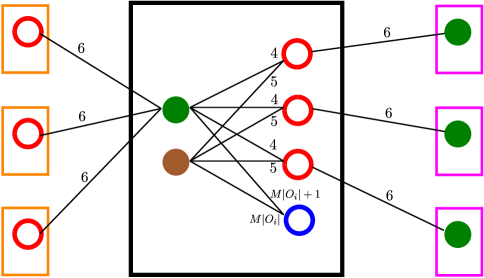
Figure 1: A diagrammatic representation of the non-zero bids made and received by the buyers and goods corresponding to a particular node of the threshold game. Consider a particular node of the threshold game, represented here by the black rectangle. It has three out neighbours, depicted as orange rectangles, and three in neighbours, depicted as pink rectangles. The hollow circles represent goods and the solid circles represent buyers. Corresponding to each node of the threshold game, there is one strategic buyer, shown here in green, and one threshold buyer, shown in brown. Furthermore, for each node of the threshold game, there are three neighbour goods, shown in red, and one reciprocal good, shown in blue. The lines represent non-zero bids.

With this high level overview of the reduction in place, we move on to the rigorous construction of the throttling game $\mathcal{I}_{\mathcal{G}}$ from $\mathcal{G}$. First, $\mathcal{I}_{\mathcal{G}}$ contains the following set of goods:

• For each $i\in[n]$ and $j\in N_{i}$, there is a neighbor good $G(i,j)$.

• For each $i\in[n]$, there is a reciprocal good $R(i)$.

Next, setting two constants $M$ and $\delta$ as $M={160}/{\delta}$ and $\delta=\min\{\epsilon/(3+\epsilon),\epsilon/2,1/4\},$ the throttling game $\mathcal{I}_{\mathcal{G}}$ has the following set of buyers:

• For each $i\in[n]$, there is a threshold buyer $T(i)$ who has budget $1/2$ and has non-zero bids only on the following goods: $b(T(i),G(i,j))=5$ for all $j\in N_{i}$; and $b(T(i),R(i))=M|O_{i}|$.

• For each $i\in[n]$, there is a strategy buyer $S(i)$ who has budget $M|O_{i}|/2$ and has non-zero bids only on the following goods: $b(S(i),R(i))=M|O_{i}|+1$; $b(S(i),G(i,j))=4$ for all $j\in N_{i}$; and $b(S(i),G(j,i))=6$ for all $j\in O_{i}$.

It is clear that $\mathcal{I}_{\mathcal{G}}$ can be constructed from $\mathcal{G}$ in polynomial time, and the number of buyers with non-zero bids for each good is at most three. Let $\theta$ be any $\delta$-approximate throttling equilibrium of $\mathcal{I}_{\mathcal{G}}$ and use it to define $(x_{i}\mathrel{\mathop{\mathchar 58\relax}}i\in[n])\in[0,1]^{n}$ as follows:

$$x_{i}=\min\big{\{}2(1-\theta_{S(i)}),1\big{\}},\quad\text{for all $i\in[n]$.}$$ (2)

To complete the reduction, we will show that $(x_{i}\mathrel{\mathop{\mathchar 58\relax}}i\in[n])$ is an $\epsilon$-approximate equilibrium of the threshold game $\mathcal{G}$. Since we are considering a particular $\theta$, we will suppress the dependence on $\theta$ of the payment made by buyer $B$ on good $G$ and simply denote it by $p(B,G)$. The next lemma notes the payment terms of buyers in $\mathcal{I}_{\mathcal{G}}$.

Lemma 12.

For all $i\in[n]$, we have

1. $p(T(i),G(i,j))=\left(1-\theta_{S(j)}\right)\theta_{T(i)}\theta_{S(i)}4$, for all $j\in N_{i}$; and $p(T(i),R(i))=0$.

2. $p(S(i),R(i))=\theta_{S(i)}\theta_{T(i)}M|O_{i}|$; $p(S(i),G(i,j))=0$, for all $j\in N_{i}$; and

   $$p(S(i),G(j,i))=\theta_{S(i)}\left[\theta_{T(j)}5\ +\ (1-\theta_{T(j)})\theta_{S(j)}4\right],\quad\text{for all $j\in O(i)$.}$$

In the next lemma, we bound the total payment made by strategy buyer $S(i)$ on the neighbor goods and provide lower bounds on the throttling parameters:

Lemma 13.

For all $i\in[n]$, we have $\theta_{S(i)}\geq(1-2\delta)/2$, $\theta_{T(i)}\geq 1/32$, and the total payment of $S(i)$ on the neighbor goods satisfies:

$$|O_{i}|\theta_{S(i)}\leq\sum_{j\in N_{i}}p(S(i),G(i,j))+\sum_{j\in O_{i}}p(S(i),G(j,i))\leq 5|O_{i}|\theta_{S(i)}$$

Proof  For $i\in[n]$, using Lemma 12, we get

$$\sum_{j\in N_{i}}p(S(i),G(i,j))+\sum_{j\in O_{i}}p(S(i),G(j,i))=\sum_{j\in O_{i}}\theta_{S(i)}\left[\theta_{T(j)}5\ +\ (1-\theta_{T(j)})\theta_{S(j)}4\right]\leq 5|O_{i}|\theta_{S(i)}.$$

Suppose $\theta_{S(i)}<(1-2\delta)/2$ for some $i\in[n]$. Then, the total payment made by $S(i)$ is at most

$$\theta_{S(i)}\theta_{T(i)}M|O_{i}|+5|O_{i}|\theta_{S(i)}<\frac{(1-2\delta)M|O_{i}|}{2}+5|O_{i}|<(1-\delta)\cdot\frac{M|O_{i}|}{2}$$

using $M>10/\delta$ by our choice of $M$. This contradicts the definition of $\delta$-approximate throttling equilibrium because $S(i)$ has a budget of $M|O_{i}|/2$. Therefore, we have $\theta_{S(i)}\geq(1-2\delta)/2$ and in particular, $\theta_{S(i)}\geq 1/4$ for all $i\in[n]$ using $\delta\leq 1/4$. Hence,

$$\sum_{j\in N_{i}}p(S(i),G(i,j))+\sum_{j\in O_{i}}p(S(i),G(j,i)) =\sum_{j\in O_{i}}\theta_{S(i)}\left[\theta_{T(j)}5\ +\ (1-\theta_{T(j)})\theta_{S(j)}4\right]$$

$$>\sum_{j\in O_{i}}\theta_{S(i)}\left[\theta_{T(j)}\theta_{S(j)}4\ +\ (1-\theta_{T(j)})\theta_{S(j)}4\right]$$

$$=4\theta_{S(i)}\cdot\sum_{j\in O_{i}}\theta_{S(j)}\geq|O_{i}|\theta_{S(i)}.$$

Suppose, $\theta_{T(i)}<1/32$. By Lemma 12 the total payment of threshold buyer $T(i)$ is at most

$$\sum_{j\in N_{i}}4\theta_{T(i)}\leq 12\theta_{T(i)}<\frac{3}{8}\leq\frac{1-\delta}{2}$$

using $|N_{i}|\leq 3$ and $\delta\geq 1/4$. Hence, we have obtained a contradiction with the definition of $\delta$-approximate throttling equilibria. Therefore, $\theta_{T(i)}\geq 1/32$.     $\sqcap$$\sqcup$

We are now ready to complete the reduction.

Lemma 14.

$(x_{i}\mathrel{\mathop{\mathchar 58\relax}}i\in[n])$, as defined in (2), is an $\epsilon$-approximate equilibrium of the threshold game $\mathcal{G}$.

Proof  Fix an $i\in[n]$. First consider the case when $\sum_{j\in N_{i}}x_{j}>0.5+\epsilon$. Assume for a contradiction that $x_{i}>\epsilon$. Then, $\theta(S(i))<1-(\epsilon/2)\leq 1-\delta$ using $\delta\leq\epsilon/2$. By the definition of $\delta$-approximate throttling equilibrium, the total payment of threshold buyer $S(i)$ is at least $(1-\delta)M|O_{i}|/2$. Combining this observation with Lemma 12 and Lemma 13, we get

$$\theta_{S(i)}\left[\theta_{T(i)}M|O_{i}|+5|O_{i}|\right]\geq(1-\delta)\cdot\frac{M|O_{i}|}{2}$$

and thus (using $\theta_{T(i)}\geq 1/32$ from Lemma 13 and our choice of $M=160/\delta$),

$$\theta_{S(i)}\geq\frac{1-\delta}{2\theta_{T(i)}+(10/M)}\geq\frac{1}{2\theta_{T(i)}}\cdot\frac{1-\delta}{1+\delta}\ \ \implies\ \ \theta_{T(i)}\theta_{S(i)}\geq\frac{1}{2(1+2\epsilon)}$$

using $\delta\leq\epsilon/2$ and $\epsilon<1$. Moreover, note that $\sum_{j\in N_{i}}x_{j}>0.5+\epsilon$ implies

$$\sum_{j\in N_{i}}2\left(1-\theta_{S(j)}\right)>(1+2\epsilon)/2$$

Combining the above statements allows us to bound the total payment of buyer $T(i)$:

$$\sum_{j\in N_{i}}\left(1-\theta_{S(j)}\right)\theta_{T(i)}\theta_{S(i)}4\geq\frac{4}{2(1+2\epsilon)}\cdot\sum_{j\in N_{i}}\left(1-\theta_{S(j)}\right)>\frac{1}{2}.$$

This yields a contradiction because $T(i)$ has budget $1/2$. Hence $x_{i}\leq\epsilon$ when $\sum_{j\in N_{i}}x_{j}>0.5+\epsilon$. Next consider the case of $\sum_{j\in N_{i}}x_{j}<0.5-\epsilon$. The budget constraint of $S(i)$ and Lemma 13 yield

$$\theta_{S(i)}\left[\theta_{T(i)}M|O_{i}|+|O_{i}|\right]\leq\frac{M|O_{i}|}{2}$$

which implies that

$$\theta_{S(i)}\left[\theta_{T(i)}M|O_{i}|+\theta_{T(i)}|O_{i}|\right]\leq\frac{M|O_{i}|}{2}\ \ \implies\ \ \theta_{T(i)}\theta_{S(i)}\leq\frac{1}{2(1+(1/M))}<\frac{1}{2}.$$ (3)

By Lemma 13, we have $\theta_{S(j)}\geq(1-2\delta)/2$ and thus, $2(1-\theta_{S(j)})\leq 1+2\delta$. Multiplying both sides by $(1-2\delta)$ yields $2(1-\theta_{S(j)})(1-2\delta)\leq 1-4\delta^{2}<1$. In other words, we have

$$2(1-\theta_{S(j)})(1-2\delta)<\min\{2(1-\theta_{S(j)}),1\}=x_{j}$$ (4)

for every $j\in[n]$. This together with $\sum_{j\in N_{i}}x_{j}<0.5-\epsilon$ implies

$$(1-2\delta)\sum_{j\in N_{i}}2\left(1-\theta_{S(j)}\right)<(1-2\epsilon)/2.$$

Therefore, we get that the total payment of $T(i)$ satisfies the following bound

$$\sum_{j\in N_{i}}\left(1-\theta_{S(j)}\right)\theta_{T(i)}\theta_{S(i)}4<\sum_{j\in N_{i}}2\left(1-\theta_{S(j)}\right)<\frac{1-2\epsilon}{2(1-2\delta)}\leq(1-\delta)\cdot\frac{1}{2}$$

using $\delta\leq\epsilon/2$. As a consequence of the definition of $\delta$-approximate throttling equilibria, we have that $\theta_{T(i)}\geq 1-\delta$. Finally, using (3) and (4), we have

$$x_{i}>2(1-\theta_{S(i)})(1-2\delta)\geq 2\left(1-\frac{1}{2\theta_{T(i)}}\right)(1-2\delta)\geq\frac{(1-2\delta)^{2}}{1-\delta}>\frac{1-4\delta}{1-\delta}\geq 1-\epsilon,$$

where the last inequality follows from $\delta\leq\epsilon/(3+\epsilon)$.     $\sqcap$$\sqcup$

This completes the reduction, and thereby the proof of Theorem 9, because we have shown that for any $\delta$-approximate throttling equilibrium of the throttling game $\mathcal{I}_{\mathcal{G}}$, the strategy $(x_{i})_{i}$ is an $\epsilon$-approximate equilibrium of the threshold game $\mathcal{G}$.

PPAD Membership of Approximate Second-Price Throttling Equilibria

Next, we show that the problem of computing a $\delta$-approximate throttling equilibrium belongs to PPAD by showing a reduction to BROUWER: the problem of computing an approximate fixed point of a Lipschitz continuous function from a $n$-dimensional unit cube to itself, which known to be in PPAD (Chen et al., 2009). Its proof is motivated by the argument for existence of exact throttling equilibria given in Theorem 8 and can be found in Appendix B.1

Theorem 15.

The problem of computing an approximate throttling equilibrium is in PPAD.

4.3 NP-hardness of Revenue Maximization under Throttling

To further strengthen our hardness result, next we establish the NP-hardness of computing the revenue-maximizing approximate throttling equilibrium. With revenue being one of the primary concerns of advertising platforms, this result provides further evidence of the computational difficulties which plague throttling equilibria in second-price auctions. We begin by defining the decision version of the revenue-maximization problem.

Definition 16 (REV).

Given a throttling game $G$ and target revenue $R$ as input, decide if there exists a $\delta$-approximate throttling equilibrium of $G$, for any $\delta\in[0,1)$, with revenue greater than or equal to $R$.

Note that we allow for arbitrarily bad approximations to the throttling equilibrium by allowing $\delta$ to be any number in $[0,1)$. Theorem 17 states the problem of finding the revenue maximizing approximate throttling equilibrium is NP-hard. Its based on a reduction from 3-SAT to REV and has been relegated to Appendix B.2.

Theorem 17.

REV is NP-hard.

4.4 An Algorithm for Second-Price Throttling Equilibria with Two Buyers Per Good

Next, we contrast the hardness results of the previous subsection with an algorithm for the case when each good receives at most two non-zero bids. Since goods with only one positive bid never result in a payment, without loss of generality, we can assume that every good has exactly two buyers with positive bids. More precisely, in this subsection, we will assume that $|\{i\in[n]\mid b_{ij}>0\}|=2$ for all $j\in[m]$. This special case demarcates the boundary of tractability for computing throttling equilibria in second-price auctions: Our PPAD-hardness result (Theorem 9) holds for the slightly more general case of each good receiving at most three positive bids. We begin by describing the algorithm (Algorithm 2).

Algorithm 2 Algorithm for the Two Buyer Case

0:   Throttling game $\left(n,m,(b_{ij}),(B_{i})\right)$ and parameter $\gamma>0$

0:   $\theta_{i}=\min\{B_{i}/(2\sum_{j}b_{ij}),1\}$ for all $i\in[n]$

0:   there exists a buyer $i\in[n]$ such that $\theta_{i}<1-\gamma$ and $\sum_{j}p(\theta)_{ij}<(1-\gamma)^{3}B_{i}$:

1. For all $i\in[n]$ such that $\theta_{i}<1-\gamma$ and $\sum_{j}p(\theta)_{ij}<(1-\gamma)^{2}B_{i}$, set $\theta_{i}\leftarrow\theta_{i}/(1-\gamma)$

2. For all $i\in[n]$ such that $\sum_{j}p(\theta)_{ij}>B_{i}$, set $\theta_{i}\leftarrow(1-\gamma)\theta_{i}$

0:   $\theta$

The following theorem, whose proof can be found in Appendix B.3, establishes the correctness and polynomial runtime of Algorithm 2.

Theorem 18.

Algorithm 2 returns a $(1-3\gamma)$-approximate throttling equilibrium in time which is polynomial in the size of the instance and $1/\gamma$.

5 Comparing Pacing and Throttling

In this section, we compare two of the most popular budget management strategies: multiplicative pacing and throttling. First, we restate the definition of pacing equilibrium, as it appears in Conitzer et al. (2018, 2019). Under pacing, each buyer $i$ has a pacing parameter $\alpha_{i}$ and, she bids $\alpha_{i}b_{ij}$ on good $j$. Let $p_{j}(\alpha)$ denote the price on good $j$ when all of the buyers use pacing, i.e., $p_{j}(\alpha)$ is the highest (second-highest) element among $\{\alpha_{i}v_{ij}\}_{i}$ for first-price (second-price) auctions. Then, a tuple $((\alpha_{i}),(x_{ij}))$ of pacing parameters and allocations $x_{ij}$ is called a pacing equilibrium if the following hold:

• Only buyers with the highest bid win the good: $x_{ij}>0$ implies $\alpha_{i}v_{ij}=\max_{i}\alpha_{i}b_{ij}$.

• Full allocation of each good with a positive bid: $\max_{i}\alpha_{i}b_{ij}>0$ implies $\sum_{i\in[n]}x_{ij}=1$.

• Budgets are satisfied: $\sum_{j\in[m]}x_{ij}p_{j}(\alpha)\leq B_{i}$.

• No unnecessary pacing: $\sum_{j\in[m]}x_{ij}p_{j}(\alpha)<B_{i}$ implies $\alpha_{i}=1$.

Comparing Pacing and Throttling in First-Price Auctions

We begin with a comparison of pacing equilibria and throttling equilibria for first-price auctions. In Conitzer et al. (2019), the authors show that a unique pacing equilibrium always exists in first-price auctions and characterize it as the largest element in the collection of all budget-feasible vectors of pacing parameters. In Theorem 5, we show the analogous result for throttling using similar techniques. However, unlike pacing equilibrium, which is known to be rational Conitzer et al. (2019), there exist throttling games where the throttling equilibrium is irrational as we demonstrate through Example A. Furthermore, in Borgs et al. (2007), the authors develop tâtonnement-style dynamics similar to those described in Algorithm 1, which converge to an approximate pacing equilibrium in polynomial time. In combination with Theorem 7, this provides evidence supporting the tractability of budget management for first-price auctions.

The uniqueness of pacing equilibrium and throttling equilibrium in first-price auctions is conducive to comparison, which we carry out for revenue. More specifically, in Theorem 19, we show that the revenue under the pacing equilibrium and the throttling equilibrium are always within a multiplicative factor of 2 of each other. Let REV(PE) and REV(TE) denote the revenue under the unique pacing equilibrium and the unique throttling equilibrium respectively.

Theorem 19.

For any throttling game $\left(n,m,(b_{ij}),(B_{i})\right)$, the revenue from the pacing equilibrium and the revenue from the throttling equilibrium are always within a factor of 2 of each other, i.e., REV(PE) $\leq 2\times\text{REV(TE)}$ and REV(TE) $\leq 2\times\text{REV(PE)}$.

Proof  Consider a throttling game $\left(n,m,(b_{ij}),(B_{i})\right)$. Let $\theta=(\theta_{i})_{i}$ be the unique throttling equilibrium (TE) and $\alpha=(\alpha_{i})_{i}$ be the unique pacing equilibrium (PE) for this game. We will use $p_{j}(\theta)$ and $p_{j}(\alpha)$ to denote the (expected) payment made to the seller on good $j$ under the TE and PE respectively. Then, REV(TE) $=\sum_{j}p_{j}(\theta)$ and REV(PE) $=\sum_{j}p_{j}(\alpha)$.

First, we show that REV(PE) $\leq 2\times\text{REV(TE)}$. Let $N\coloneqq\{i\in[n]\mid\theta_{i}=1\}$ be the set of buyers who are not budget constrained under the TE. Moreover, define

$$M\coloneqq\{j\in[m]\mid\exists\ i\in N\text{ such that }i\text{ wins a non-zero fraction of }j\text{ under the PE }\alpha\}$$

Note that, since $\theta_{i}=1$ and $\alpha_{i}\leq 1$ for all $i\in N$, we get that the TE yields a higher revenue for the seller on all goods in the set $M$, i.e., $p_{j}(\theta)\geq p_{j}(\theta)$ for all $j\in N$. Therefore, REV(TE) $\geq\sum_{j\in M}p_{j}(\theta)\geq\sum_{j\in M}p_{j}(\alpha)$. Furthermore, the definition of throttling equilibrium implies that every buyer $i\notin N$ spends her entire budget $B_{i}$ under the TE. Hence, by our choice of $M$, we get $\sum_{j\notin M}p_{j}(\alpha)\leq\sum_{i\notin N}B_{i}\leq$ REV(TE). Combining the two statements yields REV(PE) $\leq 2\times\text{REV(TE)}$, as desired.

Next, we complete the proof by showing that REV(TE) $\leq 2\times\text{REV(PE)}$. Let $S=\{i\in[n]\mid\alpha_{i}=1\}$ be the set of buyers who are not budget constrained under the PE. Note that, for all $i\in S$ and $j\in[m]$, buyer $i$ bids $b_{ij}$ under the PE, which implies $p_{j}(\alpha)\geq\max_{i\in S}b_{ij}$ for all goods $j\in[m]$. Therefore, for any good $j\in[m]$, the total payment made by buyers in the set $S$ under the TE is at most $p_{j}(\alpha)$. As a consequence, the total payment made by buyers in $S$ under the TE is at most REV(PE). Furthermore, the buyers not in $S$ completely spend their budget under the TE so the total payment made by buyers not in $S$ under the TE is also at most REV(PE). Hence, we have the desired inequality REV(TE) $\leq 2\times\text{REV(PE)}$.     $\sqcap$$\sqcup$

In Appendix C, we give examples to demonstrate that REV(TE) can be arbitrarily close to $2\times\text{REV(PE)}$, and REV(PE) can be arbitrarily close to $(4/3)\times\text{REV(TE)}$. In other words, for Theorem 19, the inequality REV(TE) $\leq 2\times\text{REV(PE)}$ is tight and the inequality REV(PE) $\leq 2\times\text{REV(TE)}$ is not too loose.

Comparing Pacing and Throttling for Second-Price Auctions

This subsection is devoted to the comparison of pacing equilibria and throttling equilibria in second-price auctions. We begin by noting that, in stark contrast to first-price auctions, there could be infinitely many throttling equilibria for second-price auctions as the following example demonstrates.

Example  There are 2 goods and 2 buyers. The bids are given by $b_{11}=b_{22}=2$, $b_{12}=b_{21}=1$, and the budgets are given by $B_{1}=B_{2}=1/2$. Then, it is straightforward to check that any pair of throttling parameters $\theta_{1},\theta_{2}\in[1/2,1]$ such that $\theta_{1}\theta_{2}=1/2$ forms a throttling equilibrium.     $\sqcap$$\sqcup$

Conitzer et al. (2018) demonstrate that multiplicity (although only finitely-many different equilibria) also shows up for pacing equilibria in second-price auctions, which in combination with the multiplicity of throttling equilibria bodes unfavorably for potential comparisons of revenue. The similarities do not end with multiplicity: the problems of computing an approximate pacing equilibrium and computing an approximate throttling equilibrium are both PPAD-complete (Chen et al., 2021). As a consequence, we get that, unlike first-price auctions, no dynamics can converge to an approximate equilibrium in polynomial time for second-price auctions under either budget-management approach (assuming PPAD-hard problems cannot be solved in polynomial time). Furthermore, finding the revenue maximizing throttling equilibrium and finding the revenue maximizing pacing equilibrium are both NP-hard problems (Conitzer et al., 2018). However, unlike throttling equilibria, a rational pacing equilibrium always exists (Chen et al., 2021).

6 Price of Anarchy

In this section, we study the efficiency of throttling equilibria in first-price and second-price auctions. We will use liquid welfare (Dobzinski and Leme, 2014) to measure efficiency. It is an alternative to social welfare which is more suitable for settings with budget constraints, and it reduces to social welfare when budgets are infinite.

Definition 20.

For an allocation $y=\{y_{ij}\}$, where $y_{ij}\in[0,1]$ denotes the probability of allocating good $j$ to buyer $i$, its liquid welfare $\operatorname{LW}(x)$ is defined as

$$\operatorname{LW}(y)=\sum_{i=1}^{n}\min\left\{\sum_{j=1}^{m}b_{ij}y_{ij},B_{i}\right\}$$

Remark.  Liquid welfare is traditionally defined as the amount of revenue that can be extracted from budget-constrained buyers with full knowledge of their values. If buyer $i$ was assumed to have value $v_{ij}$ for good $j$, this is given by

$$\sum_{i=1}^{n}\min\left\{\sum_{j=1}^{m}v_{ij}y_{ij},B_{i}\right\}\,.$$

However, since our model does not assume a valuation structure, we define $\operatorname{LW}(y)$ to capture the amount of revenue that can be extracted from budget-constrained buyers with full knowledge of their bids if no buyer could be charged more than her bid for any good. It reverts to the traditional definition when $b_{ij}=v_{ij}$.     $\sqcap$$\sqcup$

Let $y(\theta)$ denote the allocation when the buyers use the throttling parameters $\theta=(\theta_{1},\dots,\theta_{n})$, and let $\Theta^{*}$ be the set of all throttling equilibria. Price of Anarchy (Koutsoupias and Papadimitriou, 2009), which we define next, is the ratio of the worst-case liquid welfare of throttling equilibria to the best-possible liquid welfare that can be attained by any allocation. It measures the worst-case loss in efficiency incurred due the strategic behavior of agents when compared to the optimal outcome that could be achieved by a central planner.

Definition 21.

The Price of Anarchy (PoA) of throttling equilibria for liquid welfare is given by

$$\text{PoA}=\frac{\sup_{y\in(\Delta^{n})^{m}}LW(y)}{\inf_{\theta\in\Theta^{*}}\operatorname{LW}(y(\theta))}$$

We begin by establishing an upper bound on the Price of Anarchy for both first-price and second-price auctions. Its proof critically leverages the no-unnecessary-throttling condition of throttling equilibria, and is inspired by the Price of Anarchy result of Balseiro et al. (2022) for pacing equilibria.

Theorem 22.

For both first-price and second-price auctions, we have $\text{PoA}\leq 2$.

Next, we show that the upper bound on the PoA established in Theorem 22 is tight for both first-price and second-price auctions. We do so by demonstrating particular instances for which the bound is tight, starting with the second-price auction format.

Example  Consider a second-price auction with $m+1$ buyers and $m$ goods for some $m\in\mathbb{Z}_{+}$. Each of the first $m$ buyers bid $1$ for the $m$ goods respectively and have a budget of $\infty$, i.e., for $i\in[m]$, we have

$$b_{ij}=\begin{cases}1&\text{if }i=j\\ 0&\text{if }i\neq j\end{cases}\,,$$

and $B_{i}=\infty$ (any $B>2m$ would suffice). The last buyer has bid $b_{m+1,j}=m$ for each of the goods $j\in[m]$ and has a budget of $B_{m+1}=m+\epsilon$ for some small $\epsilon>0$. In any throttling equilibrium $\theta\in\Theta$, we have $\theta_{i}=1$ for all $i\in[m]$ because of the no-unnecessary-throttling condition. Since the sum of all the second-highest bids is $m$ and buyer $m+1$ has the highest bid for every good, she cannot possibly spend her entire budget of $B_{m+1}=m+\epsilon$ and we must also have $\theta_{m+1}=1$ by the no-unnecessary throttling condition. Therefore, there is a unique throttling equilibrium $\theta$ such that $\theta_{i}=1$ for all $i\in[m+1]$ and it has liquid welfare given by

$$\operatorname{LW}(y(\theta))=\left(\sum_{i=1}^{m}\min\left\{y_{ii}(\theta),B_{i}\right\}\right)+\min\left\{\sum_{j=1}^{m}m\cdot y_{m+1,j}(\theta),m+\epsilon\right\}=m+\epsilon$$

because $y_{m+1,j}(\theta)=1$ for all $j\in[m]$. On the other hand, consider the allocation $y$ such that $y_{ii}=1$ for all $i\in[m-1]$ and $y_{m+1,m}=1$. It has liquid welfare given by

$$\operatorname{LW}(y)=\left(\sum_{i=1}^{m-1}\min\left\{y_{ii},B_{i}\right\}\right)+\min\left\{m\cdot y_{m+1,m},m+\epsilon\right\}=m-1+m=2m-1\,.$$

Hence, the PoA is at least $(2m-1)/(m+\epsilon)$. As $m$ and $\epsilon$ were arbitrary, we can consider the limit when $m\to\infty$ and $\epsilon\to 0$, which yields the required lower bound of $\text{PoA}\geq 2$.     $\sqcap$$\sqcup$

Observe that in the previous example none of the buyers were throttled ($\theta_{i}=1$), which indicates that the lower bound is driven more by the second-price auction format than the specific budget management method, and applies to other methods like pacing. Next, we show that our bound is tight for first-price auctions.

Example  Consider a first-price auction with $m+1$ buyers and $m+1$ goods, for some $m\in\mathbb{Z}_{+}$. Each of the first $m$ buyers bid $1$ for the first $m$ goods respectively and bid $m$ on good $m+1$, and have a budget of $1$, i.e., for each $i\in[m]$, we have

$$b_{ij}=\begin{cases}1&\text{if }j=i\\ m&\text{if }j=m+1\\ 0&\text{otherwise}\end{cases}\,,$$

and $B_{i}=1$. Moreover, buyer $m+1$ has value $b_{m+1,m+1}=m$ for the $(m+1)$-th good and $b_{m+1,j}=0$ for all $j\in[m]$, with $B_{m+1}=\infty$.

Consider a throttling equilibrium $\theta\in\Theta$. We begin by showing that $\theta_{i}<1$ for all $i\in[m]$. For contradiction, suppose not. Let $i$ be the smallest index such that $\theta_{i}=1$. Then, buyer $i$ spends 1 on good $i$ and spends $m\cdot\prod_{k=1}^{i-1}(1-\theta_{k})>0$ on good $m+1$ (we use the lexicographic tie-breaking rule), which makes her total expenditure strictly greater than her budget of $B_{i}=1$, thereby yielding the required contradiction. Hence, $\theta_{i}<1$ for all buyers $i\in[m]$, and consequently, the no-unnecessary-throttling condition implies that their total expected expenditure is exactly 1, i.e., the following equivalent statements hold

$$\theta_{i}\cdot 1+\left(\prod_{k=1}^{i-1}(1-\theta_{k})\right)\cdot\theta_{i}\cdot m=1\quad\iff\quad\theta_{i}=\frac{1}{1+\left(\prod_{k=1}^{i-1}(1-\theta_{k})\right)\cdot m}\,.$$ (5)

Moreover, since their expenditure is $B_{i}=1$, that is also their contribution towards the liquid welfare. Let $g(i)\coloneqq\prod_{k=1}^{i}(1-\theta_{k})$ denote the probability that the first $i$ buyers do not participate. Next, observe that $\theta_{m+1}=1$ because of the no-unnecessary-throttling condition and $B_{m+1}=\infty$. Therefore, due to the lexicographic tie-breaking rule, buyer $m$ wins good $m+1$ with probability $g(m)=\prod_{k=1}^{m}(1-\theta_{k})$. Hence, the liquid welfare of $\theta$ is given by

$$\operatorname{LW}(y(\theta))=m\cdot 1+g(m)\cdot m\,$$

On the other hand, the allocation $y$ which awards good $i$ to buyer $i$ for all $i\in[m+1]$ has $\operatorname{LW}(y)=m+m=2m$. Consequently, we have

$$\text{PoA}\geq\frac{2m}{m+g(m)\cdot m}=\frac{2}{1+g(m)}\,.$$

To show $\text{PoA}\geq 2$, it suffices to show $\lim_{m\to\infty}g(m)=0$, which is what we do next. First, observe that (5) implies the following recursion for $g(\cdot)$:

$$g(i)=(1-\theta_{i})g(i-1)=\frac{\left(\prod_{k=1}^{i-1}(1-\theta_{k})\right)\cdot m}{1+\left(\prod_{k=1}^{i-1}(1-\theta_{k})\right)\cdot m}\cdot g(i-1)=\frac{g(i-1)^{2}\cdot m}{1+g(i-1)\cdot m}\,.$$

We will inductively show that $g(i)\leq 1-i/(m+\sqrt{m})$. Set $b=1/(m+\sqrt{m})$ The base case $i=1$ follows because $\theta_{1}=1/(1+m)$ (see (5)). Suppose $g(i-1)\leq 1-(i-1)/(m+\sqrt{m})$ for some $i\in[m]$. Then, we have

$$g(i)=\frac{g(i-1)^{2}\cdot m}{1+g(i-1)\cdot m}=\frac{m}{\frac{1}{g(i-1)^{2}}+\frac{m}{g(i-1)}}\leq\frac{m}{\frac{1}{(1-b(i-1))^{2}}+\frac{m}{1-b(i-1)}}=\frac{m\cdot(1-bi+b)^{2}}{1+m(1-bi+b)}\,.$$

To complete the induction, it suffices to show:

$$\frac{m\cdot(1-bi+b)^{2}}{1+m(1-bi+b)}\leq 1-bi$$

$$\iff m(1+b^{2}i^{2}+b^{2}-2bi+2b-2b^{2}i)\leq 1-bi+m(1+b^{2}i^{2}-2bi+b-b^{2}i)$$

$$\iff 1-bi+m(b^{2}i-b-b^{2})\geq 0$$

$$\iff 1-m\left(\frac{1}{m+\sqrt{m}}+\frac{1}{(m+\sqrt{m})^{2}}\right)-i\left(\frac{1}{m+\sqrt{m}}-\frac{m}{(m+\sqrt{m})^{2}}\right)\geq 0$$

$$\iff 1-m\left(\frac{1}{m+\sqrt{m}}+\frac{1}{(m+\sqrt{m})^{2}}\right)-i\left(\frac{\sqrt{m}}{(m+\sqrt{m})^{2}}\right)\geq 0$$

To see why the last inequality in the above equivalence chain holds, observe that:

$$1-m\left(\frac{1}{m+\sqrt{m}}+\frac{1}{(m+\sqrt{m})^{2}}\right)-i\left(\frac{\sqrt{m}}{(m+\sqrt{m})^{2}}\right)$$

$$\geq 1-m\left(\frac{1}{m+\sqrt{m}}+\frac{1}{(m+\sqrt{m})^{2}}\right)-m\left(\frac{\sqrt{m}}{(m+\sqrt{m})^{2}}\right)$$

$$= \frac{(m+\sqrt{m})^{2}-m(m+\sqrt{m})-m-m\sqrt{m}}{(m+\sqrt{m})^{2}}$$

$$= \frac{m^{2}+m+2m\sqrt{m}-m^{2}-m\sqrt{m}-m-m\sqrt{m}}{(m+\sqrt{m})^{2}}$$

$$= 0$$

which completes the induction. Hence, $g(m)\leq 1-m/(m+\sqrt{m})$ and $\lim_{m\to\infty}g(m)=0$, as required.     $\sqcap$$\sqcup$

7 Conclusion and Future Work

We defined the notion of a throttling equilibrium and studied its properties for both first-price and second-price auctions. Through our analysis of computational and structural properties, we found that throttling equilibria in first-price auctions satisfy the desirable properties of uniqueness and polynomial-time computability. In contrast, we showed that for second-price auctions, equilibrium multiplicity may occur, and computing a throttling equilibrium is PPAD hard. This disparity between the two auction formats is reinforced when we compare throttling and pacing: our results show that the properties of throttling equilibrium across the two formats have a striking similarity to the properties of first-price versus second-price pacing equilibrium. Finally, we also showed that the Price of Anarchy of throttling equilibria for liquid welfare is bounded above by 2 for both first-price and second-price auctions, and that this bound is tight for both auction formats. Altogether, this provides a comprehensive analysis of the equilibria which arise from the use of throttling as a method of budget management.

There are many interesting directions for future work, such as what happens when a combination of pacing and throttling-based buyers exist in the market, whether the combination of throttling and pacing behaves well for second-price auctions, whether second-price throttling equilibria can be computed efficiently under some natural assumptions on the bids, and whether the tractability of budget management in first-price auctions holds more generally beyond throttling and pacing.

Appendix A Appendix: Examples of Irrational Throttling Equilibria

First-Price Auctions:

First, we give an example for which the unique first-price throttling equilibrium is irrational.

Example  Define a throttling game as follows: There are 2 goods and 2 buyers, i.e., $m=2$ and $n=2$; $b_{11}=b_{12}=2$ and $b_{21}=1,b_{22}=3$; $B_{1}=2$ and $B_{2}=1$. Suppose, in equilibrium, the buyers use the throttling parameters $\theta_{1}$ and $\theta_{2}$. Then the payment of buyer 1 and buyer 2 are given by $2\theta_{1}+2(1-\theta_{2})\theta_{1}$ and $3\theta_{2}+(1-\theta_{1})\theta_{2}$ respectively. Therefore, for this game, in any throttling equilibrium, we have $0<\theta_{1},\theta_{2}<1$ and $\theta_{3}=1$, which implies $2\theta_{1}+2(1-\theta_{2})\theta_{1}=2$ and $3\theta_{2}+(1-\theta_{1})\theta_{2}=1$. Substituting $\theta_{1}=1/(2-\theta_{2})$ from the first equation into the second yields

$$3\theta_{2}+\theta_{2}\cdot\frac{1-\theta_{2}}{2-\theta_{2}}=1$$

which implies $4\theta_{2}^{2}-7\theta_{2}+1=0$. As $\theta_{2}<1$, Solving the quadratic gives $\theta_{2}=(7-\sqrt{33})/8$.     $\sqcap$$\sqcup$

Second-Price Auctions:

Next, we give an example for which all second-price throttling equilibria are irrational.

Example  Define a throttling game as follows:

• There are 4 goods and 3 buyers, i.e., $m=4$ and $n=3$

• $b_{11}=b_{12}=2$, $b_{14}=1$, $b_{23}=b_{24}=4$, $b_{22}=1$, $b_{31}=1$ and $b_{33}=2$

• $B_{1}=B_{2}=1$ and $B_{3}=\infty$

For this game, in any throttling equilibrium, we have $0<\theta_{1},\theta_{2}<1$ and $\theta_{3}=1$. Hence, if $\theta$ is a throttling equilibrium, then it satisfies $\theta_{1}+\theta_{1}\theta_{2}=1$ and $2\theta_{2}+\theta_{2}\theta_{1}=1$. Substituting $\theta_{1}=1/(1+\theta_{2})$ from the first equation into the second equation yields

$$2\theta_{2}+\theta_{2}\cdot\frac{1}{1+\theta_{2}}=1$$

which further implies $2\theta_{2}^{2}+2\theta_{2}-1=0$. As $\theta_{2}>0$, solving the quadratic gives $\theta_{2}=(\sqrt{3}-1)/2$.     $\sqcap$$\sqcup$

Appendix B Appendix: Missing Proofs

B.1 Proof of Theorem 15

Consider a throttling game $\left(n,m,(b_{ij}),(B_{i})\right)$ and an approximation parameter $\delta\in(0,1/2)$. Define $f\mathrel{\mathop{\mathchar 58\relax}}[0,1]^{n}\to[0,1]^{n}$ as

$$f_{i}(\theta)=\min\left\{\frac{(1-\delta/2)B_{i}}{\sum_{j}p(1,\theta_{-i})_{ij}},1\right\}=\min\left\{\frac{(1-\delta/2)B_{i}}{\max\{\sum_{j}p(1,\theta_{-i})_{ij},B_{i}/2\}},1\right\}\quad\forall\theta\in[0,1]^{n}$$

First, we prove that $f$ is $L$-Lipschitz continuous with Lipschitz constant $L=2mn\overline{B}\underline{B}^{-2}\overline{b}$, where $\overline{b}=\max_{i,j}b_{ij}$, $\overline{B}=\max_{i}B_{i}$. To achieve this, we will repeatedly use the following facts about Lipschitz functions. For Lipschitz continuous functions $f$ and $g$ with Lipschitz constants $L_{1}$ and $L_{2}$ respectively,

• $f+g$ is $L_{1}+L_{2}$-Lipschitz continuous

• If $f$ and $g$ are bounded above by $M$, then $f\cdot g$ is $M(L_{1}+L_{2})$-Lipschitz continuous

• If $f$ is bounded below by $c$, then $1/f$ is $L_{1}/c^{2}$-Lipschitz continuous

• For a constant $C$, $\max\{f,C\}$ and $\min\{f,C\}$ are both $L_{1}$-Lipschitz continuous

Observe that

$$p(1,\theta_{-i})_{ij}=\sum_{\ell\mathrel{\mathop{\mathchar 58\relax}}b_{\ell j}<b_{ij}}b_{\ell j}\theta_{\ell}\prod_{k\neq i\mathrel{\mathop{\mathchar 58\relax}}b_{kj}>b_{\ell j}}(1-\theta_{k})$$

Therefore, for all $i\in[n]$, $\theta\mapsto p(1,\theta_{-i})_{ij}$ is $(2n\overline{b})$-Lipschitz continuous, which further implies that $\theta\mapsto\sum_{j}p(1,\theta_{-i})_{ij}$ is $2mn\overline{b}$-Lipschitz continuous. Finally, due to the second equality in the definition of $f$, we get that $f$ is $(2mn\overline{B}\underline{B}^{-2}\overline{b})$-Lipschitz continuous.

Since BROUWER is in PPAD (Chen et al., 2009), to complete the proof, it suffices to show that a $(\delta\underline{B}/4m\overline{b})$-approximate fixed point $\theta^{*}$ of $f$, i.e, $\theta^{*}$ such that $\|f(\theta^{*})-\theta^{*}\|_{\infty}\leq\delta\underline{B}/4m\overline{b}$, is a $\delta$-approximate throttling equilibrium. First, note that $p(1,\theta_{-i})_{ij}\leq\overline{b}$ for all $i\in[n],j\in[m]$. Therefore, $f(\theta)_{i}\geq\underline{B}/2m\overline{b}$ for all $i\in[n]$. Hence, for $i\in[n]$, we have

$$\biggr{\lvert}1-\frac{\theta_{i}^{*}}{f_{i}(\theta^{*})}\biggr{\rvert}\leq\frac{\delta\underline{B}}{f_{i}(\theta^{*})\cdot 4m\overline{b}}\leq\frac{\delta}{2}$$

As a consequence, we get $\theta_{i}^{*}\leq(1+\delta/2)f_{i}(\theta^{*})$ and $\theta^{*}\geq(1-\delta/2)f_{i}(\theta^{*})$. The first inequality implies which in turn implies

$$\sum_{j}p(\theta^{*})_{ij}=\theta^{*}_{i}\cdot\sum_{j}p(1,\theta^{*})_{ij}\leq(1+\delta/2)(1-\delta/2)B_{i}\leq B_{i}$$

and the second one implies that if $\theta^{*}_{i}<1-\delta/2$, then

$$\sum_{j}p(\theta^{*})_{ij}=\theta^{*}_{i}\cdot\sum_{j}p(1,\theta^{*})_{ij}\geq(1-\delta/2)^{2}B_{i}\geq(1-\delta)B_{i}$$

Hence, $\theta^{*}$ is a $\delta$-approximate throttling equilibrium, thereby completing the proof.     $\sqcap$$\sqcup$

B.2 Proof of Theorem 17

Consider an instance of 3-SAT with variables $\{x_{1},\dots,x_{n}\}$ and clauses $\{C_{1},\dots,C_{m}\}$. Our goal is to define an instance $\mathcal{I}$ of REV (a throttling game $G$ and a target revenue $R$) which always has the same solution (Yes or No) as the 3-SAT instance, and has a size of the order $\text{poly}(n,m)$. We do so next, starting with an informal description to build intuition. To better understand the core motivations behind the gadgets, we will restrict our attention to exact throttling equilibria ($\delta=0$) in the informal discussion that follows. As we will see in the formal proof, the target revenue $R$ can be chosen carefully to ensure that only exact throttling equilibria can achieve the revenue $R$.

Reciprocal Gadget: Fix $i\in[n]$. Corresponding to variable $x_{i}$, there are two goods $\mathbb{A}_{i}$ and $\mathbb{B}_{i}$, and two buyers $V_{i}^{+}$ and $V_{i}^{-}$ in the throttling game $G$. Each buyer bids 1 for one of the goods and bids 2 for the other, with both buyers bidding differently on each good. Furthermore, we set the budgets of both buyers to be 1/2, and ensure that they do not spend any non-zero amount on goods other than $\mathbb{A}_{i}$ and $\mathbb{B}_{i}$. In equilibrium, this forces the throttling parameter of $V_{i}^{+}$ (which we denote by $\theta_{i}^{+}$) to be half of the reciprocal of the throttling parameter of $V_{i}^{-}$ (which we denote by $\theta_{i}^{-}$) and vice-versa. As a consequence, both throttling parameters lie in the interval $[1/2,1]$.

Binary Gadget: For each variable $x_{i}$, there are two additional goods $\mathbb{S}_{i}$ and $\mathbb{T}_{i}$, which receive a bid of 1 from buyers $V_{i}^{+}$ and $V_{i}^{-}$ respectively. The throttling game $G$ also has one unbounded buyer $U$ who has an infinite budget, and bids 2 on both goods $\mathbb{S}_{i}$ and $\mathbb{T}_{i}$. By the definition of throttling equilibria (Definition 1), the throttling parameter of $U$ is always 1 in equilibrium. Therefore, buyer $U$ wins both $\mathbb{S}_{i}$ and $\mathbb{T}_{i}$ with probability one, and pays $\theta_{i}^{+}+\theta_{i}^{-}=\theta_{i}^{+}+1/2\theta_{i}^{+}$ for it. Finally, observe that $t\mapsto t+1/2t$, when restricted to $t\in[1/2,1]$, is maximized at $t=1$ or $t=1/2$. Therefore, by appropriately choosing the target revenue $R$, we can ensure that revenue $R$ is only achieved by throttling equilibria in which exactly one of the following holds: $(\theta_{i}^{+}=1,\theta_{i}^{-}=1/2)$ or $(\theta_{i}^{+}=1/2,\theta_{i}^{-}=1)$. This allows us to interpret $\theta_{i}^{+}=1$ as setting $x_{i}=1$ and $\theta_{i}^{-}=1$ as setting $x_{i}=0$.

Clause Gadget: For each clause $C_{j}$, there is a good $\mathbb{C}_{j}$. If $C_{j}$ contains a non-negated literal $x_{i}$, then buyer $V_{i}^{+}$ bids 1 on good $\mathbb{C}_{j}$, and if it contains a negated literal $\neg x_{i}$, then buyer $V_{i}^{-}$ bids 1 on good $\mathbb{C}_{j}$. Furthermore, the unbounded buyer $U$ bids 2 on good $\mathbb{C}_{j}$, thereby always winning it. Hence, the total payment on good $\mathbb{C}_{j}$ is 1 if some literal is satisfied (corresponding throttling parameter is 1), and is 1/2 if no literal is satisfied (corresponding throttling parameters are 1/2). The rest of the reduction boils down to choosing $R$ appropriately.

Proof  [Proof of Theorem 17] Guided by the informal intuition described above, we proceed with the formal definition of the instance $\mathcal{I}$, which involves specifying the throttling game $G$ and the target revenue $R$. The throttling game $G$ consists of the following goods:

• Reciprocal Gadget: For each variable $x_{i}$, there are two goods $\mathbb{A}_{i}$ and $\mathbb{B}_{i}$.

• Binary Gadget: For each variable $x_{i}$, there are two binary goods $\mathbb{S}_{i}$ and $\mathbb{T}_{i}$.

• Clause Gadget: For each clause $C_{j}$, there is a good $\mathbb{C}_{j}$.

Moreover, $G$ has the following set of buyers:

• Corresponding to each variable $x_{i}$, there are two buyers $V_{i}^{+}$ and $V_{i}^{-}$ with non-zero bids only for the following goods:

  • $b(V_{i}^{+},\mathbb{A}_{i})=2$ and $b(V_{i}^{+},\mathbb{B}_{i})=1$

  • $b(V_{i}^{-},\mathbb{A}_{i})=1$ and $b(V_{i}^{-},\mathbb{B}_{i})=2$

  • $b(V_{i}^{+},\mathbb{S}_{i})=1$

  • $b(V_{i}^{-},\mathbb{T}_{i})=1$

  • $b(V_{i}^{+},\mathbb{C}_{j})=1$ if $x_{i}$ is a literal in $C_{j}$

  • $b(V_{i}^{-},\mathbb{C}_{j})=1$ if $\neg x_{i}$ is a literal in $C_{j}$

  Moreover, the budget of both $V_{i}^{+}$ and $V_{i}^{-}$ is $1/2$ for all $i\in[n]$.

• There is one unbounded buyer $U$ with $b(U,\mathbb{C}_{j})=2$ for all $j\in[m]$ and $b(U,\mathbb{S}_{i})=b(U,\mathbb{T}_{i})=2$ for all $i\in[n]$. Moreover, $U$ has a budget of $\infty$.

Set the target revenue to be $R=n+m+(3n/2)$. Suppose there exists a $\delta$-approximate throttling equilibrium $\Theta$, for some $\delta\in[0,1)$, with revenue greater than or equal to $R$. Let $\theta_{i}^{+}$ and $\theta_{i}^{-}$ denote the throttling parameters of $V_{i}^{+}$ and $V_{i}^{-}$ in $\Theta$. Then, $\theta_{i}^{+}\theta_{i}^{-}\leq 1/2$ by virtue of the budget constraints. Therefore, the revenue from goods $\{\mathbb{A}_{i}\}_{i=1}^{n}\cup\{\mathbb{B}_{i}\}_{i=1}^{n}$ is at most $n$. Furthermore, it is easy to see that the revenue from goods $\{\mathbb{C}_{j}\}_{j=1}^{m}$ is at most $m$. Additionally, the total payment by buyer $U$ on goods $\mathbb{S}_{i}$ and $\mathbb{T}_{i}$ is at most $\theta_{i}^{+}+\theta_{i}^{-}\leq\theta_{i}^{+}+(1/2\theta_{i}^{+})$. Note that $\theta_{i}^{+}+(1/2\theta_{i}^{+})$ is maximized at $\theta_{i}^{+}=1/2$ or $\theta_{i}^{+}=1$, with a value of $\theta_{i}^{+}+(1/2\theta_{i}^{+})=3/2$. Therefore, the revenue from goods $\{\mathbb{S}_{i}\}_{i=1}^{n}\cup\{\mathbb{T}_{i}\}_{i=1}^{n}$ is at most $3n/2$. Hence, the total payment made on all the goods is at most $R$.

For the total revenue under $\Theta$ to be greater than or equal to $R$, the revenue from $\{\mathbb{S}_{i}\}_{i=1}^{n}\cup\{\mathbb{T}_{i}\}_{i=1}^{n}$ must be at least $3n/2$ and the revenue from $\{\mathbb{C}_{j}\}_{j=1}^{m}$ must be at least $m$. Hence, under $\Theta$, buyer $U$ has a throttling parameter of $1$, and for each $i\in[n]$, either $(\theta_{i}^{+}=1,\theta_{i}^{-}=1/2)$ or $(\theta_{i}^{+}=1/2,\theta_{i}^{-}=1)$. Furthermore, the payment made by buyer $U$ on $\mathbb{C}_{j}$ is 1 for every $j\in[m]$. This allows us to assign values to the variables as follows: set $x_{i}=1$ if $\theta_{i}^{+}=1$ and $x_{i}=0$ if $\theta_{i}^{-}=1$. With this assignment of the variables, each clause is satisfied since the payment made by buyer $U$ on $\mathbb{C}_{j}$ is 1 for all $j\in[m]$. Hence, we have shown that if there exists a $\delta$-approximate throttling equilibrium with revenue $R$ or greater, then there exists a satisfying assignment for the 3-SAT instance.

Conversely, note that if there exists a satisfying assignment for the 3-SAT instance, then setting $\theta_{i}^{+}=1$, $\theta_{i}^{-}=1/2$ if $x_{i}=1$ and $\theta_{i}^{+}=1/2$, $\theta_{i}^{-}=1$ if $x_{i}=0$ yields a throttling equilibrium with revenue equal to $R$. To complete the proof, observe that the size of the instance $|\mathcal{I}|=\text{poly}(n,m)$.     $\sqcap$$\sqcup$

B.3 Proof of Theorem 18

In this appendix, we analyze the correctness and runtime of Algorithm 2. To do so, we will make repeated use of the following crucial observation:

$$p(\theta)_{ij}=\begin{cases}\theta_{i}\theta_{k}b_{kj}&\text{if }b_{ij}>b_{kj}>0\ \text{for some }k\in[n]\\ 0&\text{otherwise}\end{cases}$$ (6)

In particular, this observation implies that $p(1,\theta_{i})$ is a linear function of $\theta$.

The following lemma makes a step towards the proof of correctness of the algorithm by showing that the budget constraints are always satisfied.

Lemma 23.

At the start of each iteration of the while loop, we have $\sum_{j}p(\theta)_{ij}\leq B_{i}$ for all $i\in[n]$.

Proof  We will use induction on the number of iterations of the while loop to prove this lemma. By our choice of initialization of $\theta$, the budget constraints are satisfied before the first iteration of the while loop. Suppose the constraints are satisfied before the start of the $t$-th iteration and the value of $\theta$ at that stage is $\theta^{(0)}$. We will use $\theta^{(1)}$ and $\theta^{(2)}$ to the denote the value of $\theta$ after step 1 and step 2 of the $t$-th iteration respectively. Consider a buyer $i$ such that $\sum_{j}p(\theta^{(1)})_{ij}>B_{i}$. By equation 6, we get

$$B_{i}<\sum_{j}p(\theta^{(1)})_{ij}\leq\left(\sum_{j}p(\theta^{(0)})_{ij}\right)/(1-\gamma)^{2}$$

which further implies $\sum_{j}p(\theta^{(0)})_{ij}>(1-\gamma)^{2}B_{i}$. Therefore, the throttling parameter of buyer $i$ was not changed in step 1 of the $t$-th iteration, i.e., $\theta_{i}^{(0)}=\theta_{i}^{(1)}$. As a consequence, we get

$$\sum_{j}p(\theta^{(1)})_{ij}\leq\left(\sum_{j}p(\theta^{(0)})_{ij}\right)/(1-\gamma)$$

After step 2 of the $t$-th iteration, we get $\theta^{(2)}=(1-\gamma)\theta^{(1)}$. Hence,

$$\sum_{j}p(\theta^{(2)})_{ij}\leq(1-\gamma)\sum_{j}p(\theta^{(1)})_{ij}\leq\left(\sum_{j}p(\theta^{(0)})_{ij}\right)\leq B_{i}$$

where the last inequality follows from our inductive hypothesis. As $\theta^{(2)}$ is the value of $\theta$ after the $t$-th iteration, the lemma follows by induction.     $\sqcap$$\sqcup$

The next lemma establishes that the algorithm never loses any progress, i.e., any buyer who satisfies the ‘Not too much unnecessary throttling condition’ of Definition 2 at the beginning of some iteration of the while loop continues to do so at the end of it.

Lemma 24.

If $\sum_{j}p(\theta)_{ij}\geq(1-\gamma)^{3}B_{i}$ or $\theta_{i}\geq 1-\gamma$ at the start of some iteration of the while loop, then $\sum_{j}p(\theta)_{ij}\geq(1-\gamma)^{3}B_{i}$ or $\theta_{i}\geq 1-\gamma$ at the end of that iteration.

Proof  Consider an iteration of while loop which starts with $\theta=\theta^{(0)}$. We will use $\theta^{(1)}$ and $\theta^{(2)}$ to the denote the value of $\theta$ after step 1 and step 2 of this iteration. If $\sum_{j}p(\theta^{(0)})_{ij}\geq(1-\gamma)^{2}B_{i}$ at the beginning of the iteration, then $\sum_{j}p(\theta^{(2)})_{ij}\geq(1-\gamma)^{3}B_{i}$ because

$$\sum_{j}p(\theta^{(1)})_{ij}\geq(1-\gamma)^{2}B_{i}\quad\text{and}\quad\sum_{j}p(\theta^{(2)})_{ij}\geq(1-\gamma)\sum_{j}p(\theta^{(1)})_{ij}$$

Suppose $(1-\gamma)^{3}B_{i}\leq\sum_{j}p(\theta^{(0)})_{ij}<(1-\gamma)^{2}B_{i}$ and $\theta^{(0)}_{i}<1-\gamma$ at the start of the iteration. Then, after step 1, we have $(1-\gamma)^{2}B_{i}\leq\sum_{j}p(\theta^{(1)})_{ij}\leq B_{i}$. Hence, after step 2, we get $(1-\gamma)^{3}B_{i}\leq\sum_{j}p(\theta^{(3)})_{ij}$.

Finally, suppose $(1-\gamma)^{3}B_{i}\leq\sum_{j}p(\theta^{(0)})_{ij}<(1-\gamma)^{2}B_{i}$ and $\theta^{(0)}_{i}\geq 1-\gamma$ at the start of the iteration. Then, after step 1, we have $\sum_{j}p(\theta^{(1)})_{ij}\leq B_{i}$. Hence, after step 2, we still have $\theta^{(2)}_{i}\geq(1-\gamma)$. This completes the proof of the lemma.     $\sqcap$$\sqcup$

Finally, we combine the above lemmas to establish the correctness and polynomial-runtime of the algorithm.

Proof  [Proof of Theorem 18] Let $\theta^{*}$ be the vector of throttling parameters returned by the algorithm. Lemma 23 implies that $\theta^{*}$ satisfies the budget constraints of every buyer. Furthermore, upon combining $(1-\gamma)^{3}\geq 1-3\gamma$ with the termination condition of the while loop, we get that either $\theta^{*}_{i}\geq 1-\gamma$ or $\sum_{j}p(\theta^{*})_{ij}\geq(1-3\gamma)B_{i}$ for all $i\in[n]$, which makes $\theta^{*}$ a $(1-3\gamma)$-approximate throttling equilibrium.

Next, we bound the running time of the algorithm. Define $c=\min_{i}\min\{B_{i}/(2\sum_{j}b_{ij}),1\}$. Note that $c\leq\theta_{i}\leq 1$ for all $i\in[n]$ for the entire run of the algorithm. Based on Lemma 24, we define

$$A(\theta)\coloneqq\{i\in[n]\mid\sum_{j}p(\theta)_{ij}\geq(1-\gamma)^{3}B_{i}\text{ or }\theta_{i}\geq 1-\gamma$$

Then Lemma 24 simply states that if $i\in A(\theta)$ at the start of iteration $T$ of the while loop, then $i\in A(\theta)$ at the start of all future iterations $t\geq T$. Moreover, recall that the while loop terminates when $A(\theta)=[n]$.

Observe that, in each iteration of the while loop, $\theta_{i}\leftarrow\theta_{i}/(1-\gamma)$ for some $i\notin A(\theta)$. Hence, the total number of iterations of the while loop $T$ satisfies the following equivalent statements:

$$\frac{c}{(1-\gamma)^{T/n}}\leq 1\iff T\leq\frac{n\log(1/c)}{\log(1/(1-\gamma))}\leq\frac{n\log(1/c)}{\gamma}$$

This completes the proof because each iteration takes polynomially many steps.     $\sqcap$$\sqcup$

B.4 Proof of Theorem 22

Fix a throttling equilibrium $\theta\in\Theta$. Recall that we use $X=(X_{1},\dots,X_{n})$ to capture the random profile of buyers who participate in the auctions, where $X_{i}=1$ if and only if buyer $i$ participates in the auctions, and $\Pr(X_{i}=1)=\theta_{i}$. Let $y_{ij}(X)$ be the indicator random variable which equals 1 if and only if good $j$ is allocated to buyer $i$ under the participation profile $X=(X_{1},\dots,X_{n})$, and is zero otherwise. Moreover, let $p_{j}(X)$ denote the price of item $j$ under the participation profile $X=(X_{1},\dots,X_{n})$. Here, the price is the highest/second-highest bid for first-price/second-price auctions respectively, and is interpreted to be 0 if no buyers bid in an auction. Observe that

$$p_{ij}(\theta)=\mathbb{E}\left[p_{j}(X)y_{ij}(X)\right]\,.$$

Fix a benchmark allocation $y=\{y_{ij}\}$. We begin by establishing the following lemma, which will play a critical role in the proof of the theorem.

Lemma 25.

For all $i\in[n]$, we have

$$\min\left\{\mathbb{E}\left[\sum_{j=1}^{m}b_{ij}y_{ij}(X)\right],B_{i}\right\}\geq\min\left\{\sum_{j=1}^{m}b_{ij}y_{ij},B_{i}\right\}-\mathbb{E}\left[\sum_{j=1}^{m}p_{j}(X)y_{ij}\right]\,.$$

Proof  We consider two cases. First assume that $\theta_{i}<1$. Then, the no-unnecessary-throttling condition implies that $\sum_{j=1}^{m}p_{ij}(\theta)=B_{i}$. Now, observe that $y_{ij}(X)>0$ only if $b_{ij}\geq p_{j}(X)$. Consequently, we have

$$\mathbb{E}\left[\sum_{j=1}^{m}b_{ij}y_{ij}(X)\right]\geq\mathbb{E}\left[\sum_{j=1}^{m}p_{j}(X)y_{ij}(X)\right]=\sum_{j=1}^{m}p_{ij}(\theta)=B_{i}\,.$$

Hence, we get

$$\min\left\{\mathbb{E}\left[\sum_{j=1}^{m}b_{ij}y_{ij}(X)\right],B_{i}\right\} =B_{i}$$

$$\geq\min\left\{\sum_{j=1}^{m}b_{ij}y_{ij},B_{i}\right\}$$

$$\geq\min\left\{\sum_{j=1}^{m}b_{ij}y_{ij},B_{i}\right\}-\mathbb{E}\left[\sum_{j=1}^{m}p_{j}(X)y_{ij}\right]\,,$$

thereby establishing the required lemma statement for a buyer $i$ such that $\theta_{i}<1$.

Next, consider a buyer $i$ such that $\theta_{i}=1$, i.e., buyer $i$ always participates. Since $p_{j}(X)>b_{ij}$ whenever $y_{ij}(X)<1$, we have

$$0\geq\mathbb{E}\left[(b_{ij}-p_{j}(X))(1-y_{ij}(X))y_{ij}\right]\,.$$

Moreover, we also have

$$\mathbb{E}\left[b_{ij}y_{ij}(X)\right]\geq\mathbb{E}\left[(b_{ij}-p_{j}(X))y_{ij}(X)y_{ij}\right]$$

Adding the two inequalities, we get

$$\mathbb{E}\left[b_{ij}y_{ij}(X)\right] \geq\mathbb{E}\left[(b_{ij}-p_{j}(X))(1-y_{ij}(X))y_{ij}\right]+\mathbb{E}\left[(b_{ij}-p_{j}(X))y_{ij}(X)y_{ij}\right]=\mathbb{E}\left[(b_{ij}-p_{j}(X))y_{ij}\right]\,.$$

Summing over all goods $j\in[m]$ yields

$$\mathbb{E}\left[\sum_{j=1}^{m}b_{ij}y_{ij}(X)\right] \geq\sum_{j=1}^{m}b_{ij}y_{ij}-\mathbb{E}\left[\sum_{j=1}^{m}p_{j}(X)y_{ij}\right]$$

$$\geq\min\left\{\sum_{j=1}^{m}b_{ij}y_{ij},B_{i}\right\}-\mathbb{E}\left[\sum_{j=1}^{m}p_{j}(X)y_{ij}\right]$$

Additionally, we also have

$$B_{i}\geq\min\left\{\sum_{j=1}^{m}b_{ij}y_{ij},B_{i}\right\}\geq\min\left\{\sum_{j=1}^{m}b_{ij}y_{ij},B_{i}\right\}-\mathbb{E}\left[\sum_{j=1}^{m}p_{j}(X)y_{ij}\right]$$

Therefore,

$$\min\left\{\mathbb{E}\left[\sum_{j=1}^{m}b_{ij}y_{ij}(X)\right],B_{i}\right\}\geq\min\left\{\sum_{j=1}^{m}b_{ij}y_{ij},B_{i}\right\}-\mathbb{E}\left[\sum_{j=1}^{m}p_{j}(X)y_{ij}\right]\,.$$

This concludes the lemma by establishing it for buyers $i$ with $\theta_{i}=1$.     $\sqcap$$\sqcup$

With Lemma 25 in hand, we are ready to prove the theorem. First, note that

$$\sum_{i=1}^{m}\min\left\{\mathbb{E}\left[\sum_{j=1}^{m}b_{ij}y_{ij}(X)\right],B_{i}\right\} \geq\sum_{i=1}^{m}\min\left\{\sum_{j=1}^{m}b_{ij}y_{ij},B_{i}\right\}-\sum_{i=1}^{m}\mathbb{E}\left[\sum_{j=1}^{m}p_{j}(X)y_{ij}\right]$$

$$=\sum_{i=1}^{m}\min\left\{\sum_{j=1}^{m}b_{ij}y_{ij},B_{i}\right\}-\mathbb{E}\left[\sum_{j=1}^{m}p_{j}(X)\sum_{i=1}^{m}y_{ij}\right]$$

$$=\sum_{i=1}^{m}\min\left\{\sum_{j=1}^{m}b_{ij}y_{ij},B_{i}\right\}-\mathbb{E}\left[\sum_{j=1}^{m}p_{j}(X)\right]$$

$$\geq\sum_{i=1}^{m}\min\left\{\sum_{j=1}^{m}b_{ij}y_{ij},B_{i}\right\}-\mathbb{E}\left[\sum_{j=1}^{m}p_{j}(X)\sum_{i=1}^{m}y_{ij}(X)\right]$$

$$=\sum_{i=1}^{m}\min\left\{\sum_{j=1}^{m}b_{ij}y_{ij},B_{i}\right\}-\sum_{i=1}^{m}\mathbb{E}\left[\sum_{j=1}^{m}p_{j}(X)y_{ij}(X)\right]$$

where the second inequality follows from the observation that a good is always allocated whenever it has a positive bid, i.e., $\sum_{i=1}^{m}y_{ij}(X)=1$ whenever $p_{j}(X)>0$. Hence, if we can show that

$$\sum_{i=1}^{m}\min\left\{\mathbb{E}\left[\sum_{j=1}^{m}b_{ij}y_{ij}(X)\right],B_{i}\right\}\geq\sum_{i=1}^{m}\mathbb{E}\left[\sum_{j=1}^{m}p_{j}(X)y_{ij}(X)\right]\,,$$ (7)

we will get

$$\sum_{i=1}^{m}\min\left\{\mathbb{E}\left[\sum_{j=1}^{m}b_{ij}y_{ij}(X)\right],B_{i}\right\}\geq\sum_{i=1}^{m}\min\left\{\sum_{j=1}^{m}b_{ij}y_{ij},B_{i}\right\}-\sum_{i=1}^{m}\min\left\{\mathbb{E}\left[\sum_{j=1}^{m}b_{ij}y_{ij}(X)\right],B_{i}\right\}$$

$$\iff \sum_{i=1}^{m}\min\left\{2\cdot\mathbb{E}\left[\sum_{j=1}^{m}b_{ij}y_{ij}(X)\right],B_{i}\right\}\geq\sum_{i=1}^{m}\min\left\{\sum_{j=1}^{m}b_{ij}y_{ij},B_{i}\right\}\,$$

and thereby complete the proof, because the benchmark allocation $y$ and the throttling equilibrium $\theta$ are both arbitrary. In the remainder, we establish (7).

Since $y_{ij}(X)>0$ only when $b_{ij}\geq p_{j}(X)$, we have

$$\mathbb{E}\left[\sum_{j=1}^{m}b_{ij}y_{ij}(X)\right]\geq\mathbb{E}\left[\sum_{j=1}^{m}p_{j}(X)y_{ij}(X)\right]\,.$$

Moreover, the budget constraint of buyer $i$ implies

$$B_{i}\geq\mathbb{E}\left[\sum_{j=1}^{m}p_{j}(X)y_{ij}(X)\right]\,.$$

Combining the two inequalities, we get:

$$\min\left\{\mathbb{E}\left[\sum_{j=1}^{m}b_{ij}y_{ij}(X)\right],B_{i}\right\}\geq\mathbb{E}\left[\sum_{j=1}^{m}p_{j}(X)y_{ij}(X)\right]\,.$$

Summing over all buyers $i\in[n]$ yields (7), as required.

Appendix C Appendix: Examples for Section 5

First, we provide an example to show that the inequality REV(TE) $\leq 2\times\text{REV(TE)}$ is tight.

Example  Consider the throttling game in which there is 1 good and 2 buyers. The bids are given by $b_{11}=1/\epsilon$, $b_{21}=1-\epsilon$ for $\epsilon>0$ and the budgets are given by $B_{1}=1$, $B_{2}=\infty$. Then, in the unique pacing equilibrium, we have $\alpha_{1}=\epsilon$ and $\alpha_{2}=1$, whereas in the unique throttling equilibrium, we have $\theta_{1}=\epsilon$ and $\theta_{2}=1$. Hence, REV(PE) = 1 and REV(TE) = $1+(1-\epsilon)^{2}$. Since, this is true for arbitrarily small $\epsilon$, we get that the inequality REV(TE) $\leq 2\times\text{REV(TE)}$ is tight established in Theorem 19 is tight.     $\sqcap$$\sqcup$

Next, we give a family of examples for which REV(PE) is arbitrarily close to $(4/3)\times\text{REV(TE)}$.

Example  Consider a throttling game with 2 goods and 2 buyers. Fix $\epsilon>0$. The bids are given by $b_{11}=1+\epsilon$, $b_{12}=1$ and $b_{21}=1$. Moreover, the budgets are given by $B_{1}=1-\epsilon$ and $B_{2}=\infty$. Then, the unique pacing equilibrium is given by $\alpha_{1}=1-\epsilon$, $\alpha_{2}=1$, and the unique throttling equilibrium is given by $\theta_{1}=(1-\epsilon)/(2+\epsilon)$, $\theta_{2}=1$. Since $\epsilon$ was arbitrary, we can take it to be arbitrarily small. In which case, we get REV(PE) $\simeq$ 2 and REV(PE) $\simeq$ 1.5, as desired.     $\sqcap$$\sqcup$

References

- Abhishek and Hosanagar (2013) Vibhanshu Abhishek and Kartik Hosanagar. Optimal bidding in multi-item multislot sponsored search auctions. Operations Research, 61(4):855–873, 2013.
- Agarwal et al. (2014) Deepak Agarwal, Souvik Ghosh, Kai Wei, and Siyu You. Budget pacing for targeted online advertisements at linkedin. In Proceedings of the 20th ACM SIGKDD international conference on Knowledge discovery and data mining, pages 1613–1619, 2014.
- Azar et al. (2017) Yossi Azar, Michal Feldman, Nick Gravin, and Alan Roytman. Liquid price of anarchy. In International Symposium on Algorithmic Game Theory, pages 3–15. Springer, 2017.
- (4) Santiago Balseiro and Yonatan Gur. Online advertising: Competing effectively when budget is limited. https://www.informs.org/Blogs/ManSci-Blogs/Management-Science-Review/Online-Advertising-Competing-Effectively-when-Budget-is-Limited. Accessed: 2021-06-30.
- Balseiro et al. (2017) Santiago Balseiro, Anthony Kim, Mohammad Mahdian, and Vahab Mirrokni. Budget management strategies in repeated auctions. In Proceedings of the 26th International Conference on World Wide Web, pages 15–23, 2017.
- Balseiro et al. (2021) Santiago Balseiro, Anthony Kim, Mohammad Mahdian, and Vahab Mirrokni. Budget-management strategies in repeated auctions. Operations Research, 2021.
- Balseiro and Gur (2019) Santiago R Balseiro and Yonatan Gur. Learning in repeated auctions with budgets: Regret minimization and equilibrium. Management Science, 65(9):3952–3968, 2019.
- Balseiro et al. (2015) Santiago R Balseiro, Omar Besbes, and Gabriel Y Weintraub. Repeated auctions with budgets in ad exchanges: Approximations and design. Management Science, 61(4):864–884, 2015.
- Balseiro et al. (2022) Santiago R. Balseiro, Christian Kroer, and Rachitesh Kumar. Contextual standard auctions with budgets: Revenue equivalence and efficiency guarantees. In David M. Pennock, Ilya Segal, and Sven Seuken, editors, EC ’22: The 23rd ACM Conference on Economics and Computation, Boulder, CO, USA, July 11 - 15, 2022, page 476. ACM, 2022. doi: 10.1145/3490486.3538258. URL https://doi.org/10.1145/3490486.3538258.
- Borgs et al. (2007) Christian Borgs, Jennifer Chayes, Nicole Immorlica, Kamal Jain, Omid Etesami, and Mohammad Mahdian. Dynamics of bid optimization in online advertisement auctions. In Proceedings of the 16th international conference on World Wide Web, pages 531–540, 2007.
- Charles et al. (2013) Denis Charles, Deeparnab Chakrabarty, Max Chickering, Nikhil R Devanur, and Lei Wang. Budget smoothing for internet ad auctions: a game theoretic approach. In Proceedings of the fourteenth ACM conference on Electronic commerce, pages 163–180, 2013.
- Chen and Teng (2009) Xi Chen and Shang-Hua Teng. Spending is not easier than trading: on the computational equivalence of fisher and arrow-debreu equilibria. In International Symposium on Algorithms and Computation, pages 647–656. Springer, 2009.
- Chen et al. (2009) Xi Chen, Xiaotie Deng, and Shang-Hua Teng. Settling the complexity of computing two-player nash equilibria. Journal of the ACM (JACM), 56(3):1–57, 2009.
- Chen et al. (2021) Xi Chen, Christian Kroer, and Rachitesh Kumar. The complexity of pacing for second-price auctions. In Proceedings of the 22nd ACM Conference on Economics and Computation, 2021.
- Conitzer et al. (2018) Vincent Conitzer, Christian Kroer, Eric Sodomka, and Nicolás E Stier-Moses. Multiplicative pacing equilibria in auction markets. In International Conference on Web and Internet Economics, 2018.
- Conitzer et al. (2019) Vincent Conitzer, Christian Kroer, Debmalya Panigrahi, Okke Schrijvers, Eric Sodomka, Nicolas E Stier-Moses, and Chris Wilkens. Pacing equilibrium in first-price auction markets. In Proceedings of the 2019 ACM Conference on Economics and Computation. ACM, 2019.
- Daskalakis et al. (2009) Constantinos Daskalakis, Paul W Goldberg, and Christos H Papadimitriou. The complexity of computing a Nash equilibrium. SIAM Journal on Computing, 39(1):195–259, 2009.
- Dobzinski and Leme (2014) Shahar Dobzinski and Renato Paes Leme. Efficiency guarantees in auctions with budgets. In International Colloquium on Automata, Languages, and Programming, pages 392–404. Springer, 2014.
- (19) Facebook-Guide. Your guide to facebook bid strategy. https://www.facebook.com/gms_hub/share/biddingstrategyguide_final.pdf. Accessed: 2021-06-30.
- Gaitonde et al. (2022) Jason Gaitonde, Yingkai Li, Bar Light, Brendan Lucier, and Aleksandrs Slivkins. Budget pacing in repeated auctions: Regret and efficiency without convergence. arXiv preprint arXiv:2205.08674, 2022.
- Gummadi et al. (2012) Ramakrishna Gummadi, Peter Key, and Alexandre Proutiere. Repeated auctions under budget constraints: Optimal bidding strategies and equilibria. In the Eighth Ad Auction Workshop, 2012.
- Karande et al. (2013) Chinmay Karande, Aranyak Mehta, and Ramakrishnan Srikant. Optimizing budget constrained spend in search advertising. In Proceedings of the sixth ACM international conference on Web search and data mining, pages 697–706, 2013.
- Koutsoupias and Papadimitriou (2009) Elias Koutsoupias and Christos Papadimitriou. Worst-case equilibria. Computer science review, 3(2):65–69, 2009.
- Mehta (2013) Aranyak Mehta. Online matching and ad allocation. 2013.
- Mehta et al. (2007) Aranyak Mehta, Amin Saberi, Umesh Vazirani, and Vijay Vazirani. Adwords and generalized online matching. Journal of the ACM (JACM), 54(5):22–es, 2007.
- Papadimitriou and Peng (2021) Christos Papadimitriou and Binghui Peng. Public goods games in directed networks. In Proceedings of the 22nd ACM Conference on Electronic Commerce, 2021.
- Papadimitriou (1994) Christos H Papadimitriou. On the complexity of the parity argument and other inefficient proofs of existence. Journal of Computer and system Sciences, 48(3):498–532, 1994.
- Vazirani and Yannakakis (2011) Vijay V Vazirani and Mihalis Yannakakis. Market equilibrium under separable, piecewise-linear, concave utilities. Journal of the ACM (JACM), 58(3):1–25, 2011.
- Xu et al. (2015) Jian Xu, Kuang-chih Lee, Wentong Li, Hang Qi, and Quan Lu. Smart pacing for effective online ad campaign optimization. In Proceedings of the 21th ACM SIGKDD International Conference on Knowledge Discovery and Data Mining, pages 2217–2226, 2015.
Electronic Companion: