The effect of elastic disorder on single electron transport through a buckled nanotube

Abstract

We study transport properties of a single electron transistor based on elastic nanotube. Assuming that an external compressive force is applied to the nanotube, we focus on the vicinity of the Euler buckling instability. We demonstrate that in this regime the transport through the transistor is extremely sensitive to elastic disorder. In particular, built-in curvature (random or regular) leads to the “elastic curvature blockade”: appearance of threshold bias voltage in the $I$-$V$ curve which can be larger than the Coulomb-blockade-induced one. In the case of a random curvature, an additional plateau in dependence of the average current on a bias voltage appears.

I Introduction

A global trend of modern electronics is the design of nanodevices with ultra-low power consumption and a high level of integration. One of the most attractive candidates for this purpose is a single-electron transistor (SET) which is a sensitive electronic device based on the Coulomb blockade effect. Key points of fundamental physics of SET and its operation as a tunable nanodevice have been formulated about 20 years ago (for review see [1, 2, 3, 4, 5]). There has recently been an increased interest to this topic partially associated with the discovery of carbon systems with a transverse degree of freedom, such as suspended nanotubes and graphene. The interest is motivated by creation of nanoelectromechanical systems (NEMS) which are a class of devices integrating electrical and mechanical functionality on the nanoscale [6, 7, 8, 9, 10, 11, 12, 13, 14, 15, 16, 17, 18]. The simplest model of SET-based NEMS is provided by a harmonic mechanical oscillator coupled to an excess particle number on the SET island [19, 20, 21, 22, 23, 24, 25, 16, 17, 18].

When suspended elastic nanotube is used as a SET island, coupling between mechanical and charge degrees of freedom provides an additional control via mechanical forces. This coupling can be strongly increased by applying a compressive force driving the nanotube towards the Euler buckling instability [26, 27] (see more recent experimental [29, 28, 30, 31, 32, 33, 34, 35, 36] and theoretical [37, 38, 39, 40, 16, 42, 41, 17, 43, 18, 44] studies of this instability). Physics of such systems is captured by the model developed in Refs. [16, 17, 18]. This model was focused on the study of a SET made of a clean nanotube in which fluctuations arise only due to temperature $T$. Such fluctuations lead to “elastic blockade”: appearance of a small threshold bias voltage in the SET $I$-$V$ curve at the center of Coulomb blockade peak [16, 17, 18] (the term elastic blockade was introduced earlier for other materials [8, 13]). However, the extreme sensitivity of the nanomechanical SET to an external environment implies that presence of disorder or some built-up deflection from ideal symmetry can strongly modify the elastic blockade.

Typically, nanotubes are not ideal and, therefore, are curved (in a random or regular way) in their equilibrium state. The effect of such built-in curvature is manifold. First of all, it can change the effective potential well confining electrons in the SET island and redistribute the electron density. This effect is weak provided that the curvature-induced electronic potential is small as compared to the Fermi energy. Secondly, built-in curvature can lead to an electron scattering. This effect is also weak, since a typical spacial scale of curvature is much larger than the Fermi wavelength. The most significant effect is related to the presence of elastic degree of freedom. In particular, as was shown in Refs. [42, 41, 43, 44], built-in curvature can strongly affect buckling transition.

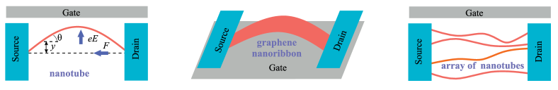
Figure 1: Sketch of a possible realization of SETs with an elastic degree of freedom. Left: A SET based on a suspended nanotube tunnel-coupled to a source and a drain and driven by an external force $F.$ A gate electrode creates additional electric field $E$ in the $y$ direction. This transverse field bends the nanotube provided it is occupied by an excessive electron. Central: A SET with a graphene nanoribbon buckled by an external force. Right: A SET made of an array of nanotubes.

These studies have a great relevance to experiment. Experimentally, the SETs with elastic degree of freedom can be realized and tested in various systems, some of which are sketched in Fig. 1. The simplest realization is a nanotube located in a plane and coupled, both electrically and mechanically, with source and drain (see the left panel of Fig. 1). Mechanical coupling leads to buckling within the same plane. Physically, this system is fully equivalent to a graphene nanoribbon, which buckles in the direction perpendicular to plane (see the central panel in Fig. 1). Additionally, electro-mechanical coupling can be studied in an array of nanotubes shown in the right panel of Fig. 1.

Recently, a possibility of a complete control of nanotube-based SETs by means of an external mechanical forces has been clearly demonstrated experimentally [33, 34, 35, 36]. In particular, in a very recent experimental work [35] a double-well elastic potential describing collective coordinate $Y$ was created and controlled mechanically by using two mechanical forces: a compressive force along the nanotube which leads to buckling bistability and a force in the perpendicular direction, which makes the double-well potential asymmetrical thus “helping” the nanotube to choose the proper potential minimum. This experimental situation exactly corresponds to the theoretical model we shall focus in this paper. In Ref. [33] the lowest-lying flexural eigenmodes of nanotube were identified with an unprecedented precision by capacitively driving the nanotube-based mechanical resonator with external circuit. Excitation of such eigenmodes by placing the nanotube into the optical cavity shows surprisingly high quality factors (up to $10^{4}!$) [34]. The latter proves extreme sensitivity of suspended nanotubes to external forces. SET coupled to oscillating field was realized in Ref. [36] and field-driven Coulomb blockade peaks were used to make a single-electron “chopper”.

In this paper, we study disordered nanotube- or nanoribbon-based SET under the action of a mechanical force (see Fig. 1). We model disorder by spontaneous local curvature (regular or random) [42, 41, 43, 44]. We demonstrate that the results obtained in Refs. [16, 17, 18] for a clean nanomechanical SET are strongly modified in the presence of such curvature. This built-in curvature leads — due to electro-mechanical coupling — to two crucial effects: (i) existence of large threshold bias voltage in $I$-$V$ curve at the center of Coulomb blockade peak for a fixed, built-in curvature (see Fig. 2), (ii) appearance of an intermediate plateau in bias-voltage dependence of the current averaged over realizations of random curvature (see bottom panel in Fig. 10).

Outline of the paper is as follows. We start with formulation of the model in Sec. II. In Sec. III the approximate treatment of the model is developed. The current for a fixed curvature of nanotube is calculated in Sec. IV. The case of a random curvature is considered in Sections V and VI. We end the paper with discussions and conclusions in Sec. VII. Some technical details are given in Appendices.

II Model

The sketch of the setup is shown in Fig. 1 (left panel). We consider a nanotube of length $L$ suspended between left and right leads, which serve as source and drain, respectively. The tunneling coupling of the nanotube to the source (drain) is characterized by the tunneling rates $\Gamma_{L}$ ($\Gamma_{R}$). We assume that a finite voltage bias $V$ is applied between source and drain shifting their chemical potentials to ${\pm}eV/2$. The electrical potential $V_{\rm g}$ of the nanotube can be tuned by a capacitively coupled electrode (gate). We consider regime of strong Coulomb blockade, $T{<}E_{\rm c},$ such that only a single excessive (in addition to a quasi-neutral Fermi gas) electron can occupy a nanotube. Here, $E_{c}$ is the charging energy ($E_{\rm c}{\sim}10$ meV for a typical nanotube length $L{\sim}0.1~{}\mu$m). The Hamiltonian of a nanotube, including the elastic degrees of freedom parametrized by the bending angle $\theta$ as a function of the arc-length position $s$ reads

$$\hat{H}=\int_{0}^{L}ds\ \Bigl{[}\kappa(\theta^{\prime}-C^{\prime})^{2}/2+F\cos\theta\Bigr{]}+eE\hat{n}_{\rm d}Y.$$ (1)

Here $\theta^{\prime}{\equiv}{d\theta}/{ds},$ $\kappa$ denotes the bending rigidity of the nanotube, $F$ stands for the compressing force applied to the ends of the nanotube, $E$ is an additional electric field created by the gate electrode, directed along $y$ axis, and

$$Y=\int_{0}^{L}|\psi_{0}(s)|^{2}y(s)ds$$ (2)

is the average displacement of the nanotube in $y$ direction. Here, $y(s)$ is transverse coordinate of the nanotube, related to bending angle as follows,

$$\frac{dy}{ds}=\sin\theta.$$ (3)

We model disorder by built-in curvature described by function $C(s),$ which can be regular or random. The electronic degrees of freedom enters the Hamiltonian (1) via the operator of the excess particle number, $\hat{n}_{\rm d}$, and the wave function, $\psi_{0}(s)$, of an active energy level for an excessive electron on the nanotube. Provided the nanotube is occupied by an additional electron, the quasi-neutrality is broken, and the transverse electric field $E$ bends the nanotube. Hence, there is the term $eE\hat{n}_{\rm d}Y$ in Eq. (1). The nanotube is assumed to be clamped on the left and right leads of the SET, such that Hamiltonian (1) has to be supplemented by the following curvature-dependent boundary conditions [41, 42],

$$y(0)=y(L),\quad\theta^{\prime}(0)=C^{\prime}(0),\quad\theta^{\prime}(L)=C^{\prime}(L).$$ (4)

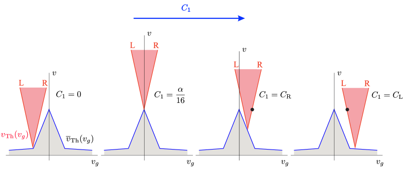
Figure 2: Schematic plot of the current density in $(v_{g},v)$ plane for different realizations of a built-in curvature, characterized by disorder strength, $C_{1}$. Disorder increases from the left panel to the right one. Regions with non-zero current, $v{>}v_{\rm Th}(v_{g}),$ are marked by pink color. They have a form of triangle with right (R) and left (L) boundaries described by function $v_{\rm Th}(v_{g})$ and shown by red thick lines. Small gap corresponding to zero current in the $I$-$V$ curve in the clean case, $C_{1}=0,$ is dramatically increased in the certain interval of disorder strength, and is maximal for $C_{1}{=}\alpha/16$ due to the elastic curvature blockade. For any point in $(v_{g},v)$ plane there are two values of disorder $C_{1}{=}C_{\rm R}$ and $C_{1}{=}C_{\rm L}$ corresponding to crossing of this point, respectively, by the right and left boundaries of the current-carrying triangle ($C_{\rm L}{>}C_{\rm R}$). Both $C_{\rm L}$ and $C_{\rm R}$ depend on coordinates $v_{g},v$, $C_{\rm R,L}{=}C_{\rm R,L}(v_{g},v).$ Area where current is zero for any disorder, $v{<}\overline{v}_{\rm Th}(v_{g})$ is marked by grey color. The function $\overline{v}_{\rm Th}(v_{g})$ is shown by thick blue line.

In the Hamiltonian (1) we neglect the elastic kinetic energy. This is justified under assumption that a typical elastic frequency of transverse oscillations of the nanotube, $\omega{\propto}\sqrt{\kappa/(\rho L^{4})}$, where $\rho$ is the linear mass density of the nanotube, is small as compared to temperature, $\hbar\omega{\ll}T$. As a result, the only dynamical degree of freedom in the Hamiltonian (1) is the excess particle number, $\hat{n}_{\rm d}$. In the strong Coulomb blockade regime, the operator $\hat{n}_{\rm d}$ takes two values, $n_{\rm d}{=}0$ and $n_{\rm d}{=}1$. Solution of the coupled — electronic and elastic — dynamical problem can be essentially simplified in the adiabatic approximation provided the tunneling between the nanotube and the source and the drain is sufficiently fast, $\Gamma_{\rm L,R}{\gg}\omega$. In such adiabatic approximation and under assumption, $\hbar\Gamma_{\rm R,L}{\ll}\max\{T,|eV|,|eV_{g}|\}$, the computation of the bending angle becomes fully classical and the bending angle profile is described by the following nonlinear equation (for $C(s){\equiv}0,$ this equation was derived in Ref. [17])

$$\kappa\left[\theta^{\prime\prime}(s)-C^{\prime\prime}(s)\right]\!+\!F\sin\theta(s)=eE(s)n_{\rm d}(Y)\cos\theta(s),$$ (5)

where $E(s){=}E\int_{s}^{L}ds^{\prime}|\psi_{0}(s^{\prime})|^{2}$ and $n_{\rm d}(Y)$ is the average value of the operator $\hat{n}_{\rm d}$ for a fixed configuration $\theta(s)$,

$$n_{\rm d}(Y)=\sum\limits_{\lambda=\pm}\gamma_{\lambda}f_{\rm F}\bigl{(}eEY-eV_{\lambda}\bigr{)}.$$ (6)

Here $f_{\rm F}(\varepsilon){=}1/[\exp(\varepsilon/T){+}1]$ denotes the Fermi function, $V_{\pm}=V_{\rm g}\pm V/2$, $\gamma_{-}{=}\Gamma_{\rm L}/(\Gamma_{\rm L}{+}\Gamma_{\rm R})$, and $\gamma_{+}{=}\Gamma_{\rm R}/(\Gamma_{\rm L}{+}\Gamma_{\rm R}).$ Under the same assumptions, the SET current reads

$$\mathcal{I}=\frac{2e\Gamma_{R}\Gamma_{L}I(Y)}{\Gamma_{L}+\Gamma_{R}},\quad I(Y){=}\sum\limits_{\lambda{=}\pm}\frac{\lambda}{2}f_{\rm F}\bigl{(}eEY-eV_{\lambda}\bigr{)}.$$ (7)

In order to compute the current by means of Eq. (7), one needs to solve the nonlinear second order differential Eq. (5). Although it can be done numerically, as we shall demonstrate below, one can construct an analytic solution near buckling instability.

III Fundamental mode approximation

In order to satisfy the boundary conditions (4), it is convenient to expand the functions $\theta(s)$ and $C(s)$ in the Fourier series,

$$\theta(s)=\sum\limits_{n=1}^{\infty}\theta_{n}\cos q_{n}s,\quad C(s)=\sum\limits_{n=1}^{\infty}C_{n}\cos q_{n}s,$$ (8)

where $q_{n}{=}\pi n/L$. Euler buckling instability is clearly seen from Eq. (5) at $E{=}0$. Indeed, linearization of this equation yields divergence of $\theta_{1}$, for $F{=}F_{\rm c}$:

$$\theta_{1}\approx-\frac{8C_{1}}{\epsilon},\quad\epsilon=\frac{8(F-F_{\rm c})}{F_{\rm c}},\quad F_{\rm c}{=}\kappa\left(\frac{\pi}{L}\right)^{2},$$ (9)

for the critical force of the instability (see Refs. [26, 27]).

Hereafter we assume that $|\epsilon|{\ll}1$. In fact, the growth of $\theta_{1}$ for $|\epsilon|{\to}0$ is limited by nonlinear terms in the Eq. (5). The modes $\theta_{n}$ with $n{\geqslant}2$ are finite at $F{=}F_{\rm c}$ and can be found within the linear approximation: $\theta_{n}{\sim}C_{n}$. Such crucial difference between the behavior of the mode with $n{=}1$ and modes with $n{\geqslant}2$ allows us to project Eq. (5) onto the fundamental mode $\cos(q_{1}s)$ as it was done in the clean case [16, 17]. In the most of our paper, we throw out all but the first mode (weak effects coming from modes with $n{\geqslant}2$ are briefly discussed at the Appendix A). The shape of nanotube, within fundamental mode approximation can be found from Eq. (3) and is given by

$$y_{1}(s)=\frac{L\theta_{1}}{\pi}\sin\left(\frac{\pi s}{L}\right).$$ (10)

We shall also make several simplifying assumptions throughout the paper. We assume the symmetric SET, $\Gamma_{R}{=}\Gamma_{L}{=}\Gamma$ (i.e., $\gamma_{+}{=}\gamma_{-}{=}1/2$). Also we set $T{=}0$. We shall estimate the effect of thermal fluctuations at the end of the paper and demonstrate that for realistic values of parameters this effect is small. The latter assumption allows one to replace Fermi functions entering Eqs. (6) and (7) with step-functions. We shall also assume that disorder is weak so that $|\theta_{1}|{\ll}1.$ Then, expanding sinus in Eq. (5) as $\sin\theta{\approx}\theta{-}\theta^{3}/6,$ keeping only the first harmonic, $\theta{\approx}\theta_{1}\cos(q_{1}s),$ and projecting thus obtained equation onto the first mode, we obtain the closed nonlinear balance equation for the amplitude of the first harmonic $\theta_{1}$:

$$f(\theta_{1})=0,$$ (11)

where

$$f(\theta_{1}) =\theta_{1}^{3}-\epsilon\theta_{1}+\alpha n_{\rm d}(\theta_{1})-8C_{1},$$ (12)

$$n_{\rm d}(\theta_{1}) =\frac{1}{2}\left[\Theta(v_{+}-\theta_{1})+\Theta(v_{-}-\theta_{1})\right].$$ (13)

Here $\Theta(x)$ denotes the Heaviside step function. Within the same approximation the current is given by

$$\mathcal{I}=e\Gamma I(\theta_{1}),\quad I(\theta_{1}){=}\frac{1}{2}\left[\Theta(v_{+}{-}\theta_{1}){-}\Theta(v_{-}{-}\theta_{1})\right].$$ (14)

In Eqs.  (12), (13), and (14) we introduced dimensionless strength of the electron-phonon interaction and the dimensionless voltages [45]

$$\alpha=\frac{16a_{1}eE}{\pi F_{\rm c}},\quad v_{\pm}{=}v_{\rm g}{\pm}\frac{v}{2},$$ (15)

$$v_{\rm g}=\frac{\pi V_{\rm g}}{a_{1}EL},\quad v=\frac{\pi V}{a_{1}EL},$$

where $a_{1}{=}\int_{0}^{L}ds\,|\psi_{0}(s)|^{2}\sin(q_{1}s)$ is the numerical coefficient which fully encodes the dependence on the wave function of the active electron quantum level: it changes from $a_{1}{=}8/3\pi$ for $\psi_{0}(s){=}\sqrt{2/L}\sin(q_{1}s)$ to $a_{1}{\approx}2/\pi$ for $\psi_{0}(s){=}\sqrt{2/L}\sin(q_{N}s)$ with $N{\approx}k_{\rm F}L/\pi{\gg}1$. Here $k_{\rm F}$ stands for the Fermi momentum.

Importantly, the typical magnitude of $\alpha$ is very small, $\alpha{\sim}10^{-4}\div 10^{-2}$ [17], that will allow us to study the effect of the electro-mechanical coupling perturbatively.

We are interested in the solution $\theta_{1}(C_{1})$ of Eq. (11) that provides the minimum of the dimensionless energy

$$W(\theta_{1})=\frac{(\theta_{1}^{2}-\epsilon)^{2}}{4}+\alpha w_{\rm d}(\theta_{1})-8C_{1}\theta_{1},$$ (16)

related to $f(\theta_{1})$ as follows: $f(\theta_{1}){=}\partial W(\theta_{1})/\partial\theta_{1}.$ Here we introduce

$$w_{\rm d}(\theta_{1})=\int_{0}^{\theta_{1}}n_{\rm d}(\theta)d\theta=\frac{1}{2}\sum_{\lambda=\pm}(\theta_{1}-v_{\lambda})\Theta(v_{\lambda}-\theta_{1}).$$ (17)

We subtracted from $w_{\rm d}$ the $\theta_{1}-$independent term $[v_{+}\Theta(v_{+}){+}v_{-}\Theta(v_{-})]/2$ and assumed that $v_{+}{>}v_{-}$ ($v{>}0$). We note that in the single mode approximation the energy, $\mathcal{E}(\theta_{1}),$ corresponding to Hamiltonian (1) is connected with the dimensional energy $W(\theta_{1})$ as follows

$$\mathcal{E}(\theta_{1})=\frac{\pi^{2}\kappa W(\theta_{1})}{16L}.$$ (18)

For $\alpha{=}0$ the energy $W(\theta_{1})$ has the form of the Landau expansion of the free energy in series of the order parameter $\theta_{1}$ near the second order phase transition at $\epsilon{=}0$. The curvature $C_{1}$ plays the role of the symmetry-breaking field that breaks the symmetry between two states of minimal energy at $\epsilon{>}0.$ Hence, the system can show the hysteretic behavior. However, since we focus here in dc current, we assume that the system always has time to reach the absolute energy minimum.

Most importantly, the single-mode approximation allows us to find the $I$-$V$ curve for a fixed curvature (i.e. for given $C_{1}$). For random curvature which is characterized by a certain distribution function $\mathcal{P}(C_{1})$, this approximation allows us to calculate analytically the distribution function for the current and analyze the competition of the random curvature with the term $\alpha w_{\rm d}(\theta_{1}),$ which suppresses the bistablity. Below, we discuss the cases of fixed and random curvature in Sections IV and V, respectively.

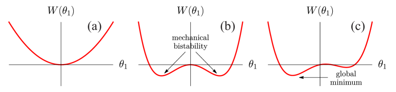
Figure 3: The effective energy for the clean nanotube at $\alpha{=}0$ below (a) and above (b) the buckling instability threshold. Above the threshold the instability leads to a mechanical bistability in the clean nanotube. Disorder breaks the symmetry between two bistable states and the global energy minimum appears (c), which depends on a specific disorder realization.

IV Current for a given curvature

In order to calculate $\theta_{1}$ for fixed value of $C_{1}$ one needs to find all solutions of the balance Eq. (11), calculate corresponding energies with the use of Eq. (16) and find global energy minimum by choosing solution with the lowest energy.

IV.1 Clean case in the absence of electro-mechanical coupling ($C_{1}{=}0,\alpha{=}0$)

In order to set notations we start from the analysis of a clean nanotube without electromechanical coupling. Then, Eq. (11) simplifies drastically,

$$\theta_{1}^{3}-\epsilon\theta_{1}=0.$$ (19)

This equation describes conventional buckling instability [27]. It has a single stable solution, $\theta_{1}{=}0$ for $\epsilon{<}0$, and two stable solutions and an unstable one for $\epsilon{>}0$:

$$\theta_{1}=\begin{cases}\pm\sqrt{\epsilon},\quad&\text{ (stable)},\\ 0,\quad&\text{ (unstable)}.\end{cases}$$ (20)

The effective energy for $\theta_{1}$ mode looks:

$$W(\theta_{1})=\frac{(\theta_{1}^{2}-\epsilon)^{2}}{4}.$$ (21)

Function $W(\theta_{1})$ is plotted in Fig. 3a for $\epsilon{<}0$ and in Fig. 3b for $\epsilon{>}0$. As one can see, the system shows mechanical bistability above the instability threshold, $\epsilon{>}0$.

IV.2 Disordered case in the absence of electro-mechanical coupling ($C_{1}{\neq}0,\alpha{=}0$)

Disorder modifies the balance equation and the effective energy as follows

$$f(\theta_{1})=\theta_{1}^{3}-\epsilon\theta_{1}-8C_{1}=0,$$ (22)

$$W(\theta_{1})=\frac{(\theta_{1}^{2}-\epsilon)^{2}}{4}-8C_{1}\theta_{1}.$$ (23)

The effective energy for $C_{1}\neq 0$ is shown in Fig. 3c. Solutions of Eq. (22) depend on $C_{1},$ so that for $\epsilon{>}0$ and at sufficiently weak disorder there are two stable solutions, $\theta^{\pm}(C_{1})$ (see blue thick curves in Fig. 4), and one unstable solution (see dashed curve in Fig. 4), just as in the clean case. It is easy to check that $W(\theta^{+}){<}W(\theta^{-})$ for $C_{1}{>}0$ and $W(\theta^{+}){>}W(\theta^{-})$ for $C_{1}{<}0$. The dependence $\theta_{1}(C_{1})$ corresponding to the absolute energy minimum of $W(\theta_{1})$ is shown in Fig. 4 by red thick curve for $\epsilon>0.$ As seen, there is a jump at $C_{1}=0,$ corresponding to transition from $\theta^{-}$ to $\theta^{+}.$ Hence, in the case $\epsilon>0$ the dependence of $\theta_{1}$ on $C_{1}$ can be written as

$$\theta_{1}(C_{1})\!=\!\Theta(C_{1})\theta^{+}(C_{1})\!+\!\Theta(-C_{1})\theta^{-}(C_{1}).$$ (24)

IV.3 Effect of electro-mechanical coupling

For $\alpha{\neq}0,$ the step functions entering both $f(\theta_{1})$ and $W(\theta_{1})$ depend on $v_{\pm}$ [see Eqs. (12), (13), (16), and (17)]. As follows from Eqs. (13) and (17), the quantities $n_{\rm d}$ and $w_{\rm d}$ can take different values depending on relation between $\theta_{1}$ and $v_{\pm}$:

$$\begin{array}[]{ll}\displaystyle&n_{\rm d}=1,\quad w_{\rm d}=\theta_{1}-v_{g},\quad{\rm for}\quad\theta_{1}<v_{-},\\ &n_{\rm d}=\frac{1}{2},\quad w_{\rm d}=\frac{\theta_{1}-v_{+}}{2},\quad\hskip 2.84526pt{\rm for}\quad v_{-}\leqslant\theta_{1}<v_{+},\\ &n_{\rm d}=0,\quad w_{\rm d}=0,\hskip 36.98866pt{\rm for}\quad v_{+}\leqslant\theta_{1}.\end{array}$$ (25)

It is convenient to introduce three functions,

$$f_{s}(\theta_{1})=\theta_{1}^{3}-\epsilon\theta_{1}-8C_{s},\quad s=a,b,c,$$ (26)

that correspond to different possible values of $n_{\rm d}.$ Here, we denote

$$C_{a}=C_{1}-\frac{\alpha}{8},\qquad C_{b}=C_{1}-\frac{\alpha}{16},\qquad C_{c}=C_{1}.$$ (27)

These functions are shown in Fig. 5 by dashed lines. As seen from this figure, solutions of equations $f_{s}(\theta_{1}){=}0$ give (for not too large magnitudes of $C_{1}$ and $\alpha$) six values of $\theta_{1}$ (we do not consider here three unstable states with $\theta_{1}$ close to zero):

$$\theta^{\pm}_{s}=\theta^{\pm}(C_{s}),$$ (28)

where functions $\theta^{\pm}(C_{1})$ are shown in Fig. 4. We notice that only two solutions, $\theta^{\pm}_{b},$ belong to the interval $v_{-}{<}\theta_{1}{<}v_{+}$ and, therefore, correspond to nonzero current through the nanotube [see Eq. (14)]. Using Eqs. (16) and (25), one can easily find energies corresponding to the solutions $\theta_{s}^{\pm}$:

$$W_{a}^{\pm}{=}\omega_{a}^{\pm}{-}\alpha v_{g},\quad W_{b}^{\pm}{=}\omega_{b}^{\pm}{-}\alpha v_{+}/2,\quad W_{c}^{\pm}{=}\omega_{c}^{\pm},$$ (29)

$$\omega_{s}^{\pm}{=}\frac{[(\theta_{s}^{\pm})^{2}{-}\epsilon]^{2}}{4}{-}8C_{s}\theta_{s}^{\pm}.$$ (30)

Importantly, $\omega_{s}^{\pm}$ are functions of $C_{1}$ and $\alpha$ only and do not depend on $v_{g}$ and $v.$

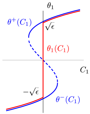
Figure 4: Schematic dependence of $\theta_{1}$ on the disorder strength $C_{1}$, corresponding to the absolute minimum of the effective energy $W$ (red curve) for $\epsilon>0.$ Blue thick curves represent two stable solutions, $\theta^{\pm}(C_{1}),$ dashed curve is the unstable solution.

Next step is to find regions in the plane $(v_{g},v),$ where one or several solutions (28) are realized and, in the case of several solutions, chose solution with the lowest energy. This procedure is illustrated in Fig. 5. Function $f(\theta_{1})$ defined by Eq. (12) is non-monotonous (see red curve in Fig. 5a) and have jumps at the points $\theta_{1}{=}v_{+}$ and $\theta_{1}{=}v_{-}.$ Equation $f(\theta_{1}){=}0$ yields several solutions for $\theta_{1}$ belonging to manifold (28). For example, in Fig. 5a the voltages $v_{\pm}$ are such that there are three solutions: $\theta_{b}^{-},\theta_{c}^{-}$ and $\theta_{c}^{+}.$ These solutions give the three local minima of the energy $W$ (see Fig. 5b). As one can see, the global minimum correspond to $\theta_{c}^{+},$ so that current through nanotube is zero. This example illustrates physical origin of the elastic blockade: local minimum $\theta_{b}^{-},$ corresponding to non-zero current, does not give absolute minimum. Hence, an electron placed in this local minimum should decrease its elastic energy by re-buckling from $\theta_{b}^{-}{\approx}{-}\sqrt{\epsilon}$ to $\theta_{c}^{+}{\approx}\sqrt{\epsilon}$ with simultaneous ”jumping out” from the current-carrying window.

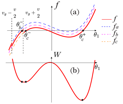
Figure 5: (a) Graphical representation of the balance equation in the presence of electro-mechanical coupling. Dashed lines represent functions $f_{a},f_{b}$ and $f_{c}$, cf. Eq. (26); red thick line shows function $f(\theta_{1})$, cf. Eq. (12)]. Equation $f(\theta_{1})=0$ have three solutions: $\theta_{b}^{-},\theta_{c}^{-}$ and $\theta_{c}^{+}.$ Only one of these solutions, $\theta_{b}^{-},$ corresponds to non-zero current through the nanotube. (b) Energy of nanotube for the same voltages. There are three local minima at $\theta_{b}^{-},\theta_{c}^{-}$ and $\theta_{c}^{+}.$ The global minimum correspond to $\theta_{c}^{+},$ so for such $v_{g}$ and $v,$ the current is blocked due to the elastic blockade.

Let us now discuss the general case. First we notice, that $(v_{g},v)$ plane can be divided onto several regions, where different solutions (28) can be realized. These regions corresponds to different regions in Eq. (25). For example, solution $\theta_{a}^{+}$ exists if $\theta_{a}^{+}{<}v_{-},$ solution $\theta_{b}^{+}$ if $v_{-}{<}\theta_{b}^{+}{<}v_{+},$ etc. Since $\theta_{s}^{\pm}$ do not depend on $v_{g}$ and $v,$ these regions are limited by lines: $v/2{=}\pm v_{g}{+}{\rm const}.$ They are shown by dashed lines in Fig. 6, where we plotted only half plane $v{>}0$ (the diagram is symmetric with respect to change $v{\to}-v$ and change $I{\to}-I$). Dashed lines connected by arrowed arcs indicates regions where different solutions (28) exist, e.g. regions $a^{\pm}$ corresponds to solutions $\theta^{\pm}_{a}$ etc. As seen, these regions overlap, so that several solutions can coexist in agreement with Fig. 5. For example, in the points $A$ three solutions coexist, $(c^{-},b^{-},c^{+}).$ Therefore, one has to calculate energies of coexisting states ($W_{c}^{-},W_{b}^{-},$ and $W_{c}^{+}$ in the above example) and to find the global minimum. Within the pink triangle in Fig. 6 the global minimum is given by one of the energies $W_{b}^{-}$ or $W_{b}^{+},$ corresponding to non-zero current, $I=1/2.$ Boundary of this triangular region, shown by two red thick lines, represents the threshold voltage, $v_{\rm Th}{=}v_{\rm Th}(C_{1},v_{g}).$ This voltage separates the region with zero current ($v{<}v_{\rm Th}$) from the region ($v{>}v_{\rm Th}$), where $I=1/2.$ Position of the triangle depends on $C_{1}$ in a non-trivial way. Analyzing Eqs. (29) and (30) one can demonstrate that the left (L) and the right (R) boundaries (red lines) are determined by the following conditions:

$$L:W_{b}^{-}{=}W_{c}^{-},\quad R:W_{b}^{-}{=}W_{a}^{-},\quad{\rm for}~{}C_{1}{<}0,$$ (31)

$$L:W_{b}^{-}{=}W_{c}^{+},\quad R:W_{b}^{-}{=}W_{a}^{-},\quad{\rm for}~{}0{\leqslant}C_{1}{<}{\alpha}/{16},$$

$$L:W_{b}^{+}{=}W_{c}^{+},\quad R:W_{b}^{+}{=}W_{a}^{-},\quad{\rm for}~{}{\alpha}/{16}{\leqslant}C_{1}{<}{\alpha}/{8},$$

$$L:W_{b}^{+}{=}W_{c}^{+},\quad R:W_{b}^{+}{=}W_{a}^{+},\quad{\rm for}~{}{\alpha}/{8}{\leqslant}C_{1}.$$

Using these relations and Eq. (29), we find that the threshold voltage can be written as follows:

$$v_{\rm Th}=v_{0}(C_{1})+2|v_{g}-v_{g0}(C_{1})|.$$ (32)

Dependence of $v_{\rm Th}{=}v_{\rm Th}(v_{g},C_{1})$ on $v_{g}$ for fixed $C_{1}$ is shown by red lines (boundaries of the current-carrying triangle) in Fig. 6. The dependence on $C_{1}$ is fully encoded in functions $v_{0}{=}v_{0}(C_{1})$ and $v_{g0}{=}v_{g0}(C_{1})$:

$$v_{0}=\frac{2}{\alpha}\left\{\begin{array}[]{ll}&2\omega_{b}^{-}{-}\omega_{c}^{-}{-}\omega_{a}^{-},\quad{\rm for}~{}C_{1}{<}0,\\ &2\omega_{b}^{-}{-}\omega_{c}^{+}{-}\omega_{a}^{-},\quad{\rm for}~{}0{\leqslant}C_{1}{<}{\alpha}/{16},\\ &2\omega_{b}^{+}{-}\omega_{c}^{+}{-}\omega_{a}^{-},\quad{\rm for}~{}{\alpha}/{16}{\leqslant}C_{1}{<}{\alpha}/{8},\\ &2\omega_{b}^{+}{-}\omega_{c}^{+}{-}\omega_{a}^{+},\quad{\rm for}~{}{\alpha}/{8}{\leqslant}C_{1},\end{array}\right.$$ (33)

$$v_{g0}=\frac{1}{\alpha}\left\{\begin{array}[]{ll}&\omega_{a}^{-}-\omega_{c}^{-},\quad{\rm for}~{}C_{1}{<}0,\\ &\omega_{a}^{-}-\omega_{c}^{+},\quad{\rm for}~{}0{\leqslant}C_{1}{<}{\alpha}/{8},\\ &\omega_{a}^{+}-\omega_{c}^{+},\quad{\rm for}~{}{\alpha}/{8}{\leqslant}C_{1},\end{array}\right.$$ (34)

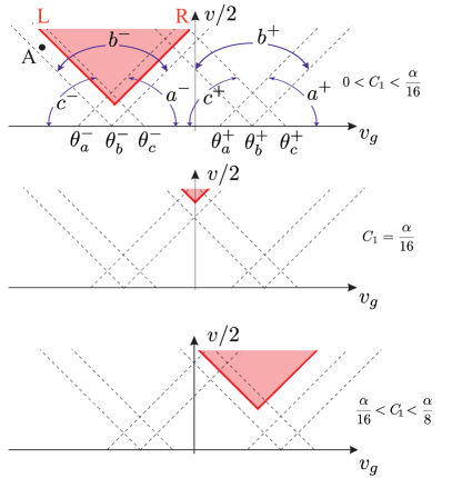
Figure 6: Phase diagram with schematically shown regions of different solutions $\theta_{s}^{\pm}.$ As seen, these regions overlap. In the area of overlapping, several solutions can coexist, giving several local minima of energy (see also Fig. 5b). Pink triangle shows the region with non-zero current. Thick red lines encode dependence of the threshold voltage $v_{\rm Th}$ on $v_{g}.$ At these lines current “jumps” from $I{=}0$ (for $v{<}v_{\rm Th}$) to $I{=}1/2$ (for $v{>}v_{\rm Th}$). The evolution of current-carrying triangle with increasing of $C_{1}$ is illustrated in top, central, and bottom panels. For $0{<}C_{1}{<}\alpha/16$ the triangle moves up (top panel), reaches maximal position at $C_{1}{=}\alpha/16$ (central panel), and moves down with further increase of disorder (bottom panel).

Equations (32), (33), and (34) provide a full solution of the problem for a fixed disorder. Functions $\omega_{s}^{\pm}$ entering these equations are given by Eq. (30) with $\theta^{\pm}_{s}$ found from Eq. (28).

For a fixed disorder the current-voltage dependence becomes

$$I(v)=\frac{{\rm sign}(v)}{2}\Theta(|v|-v_{\rm Th}).$$ (35)

Equations  (33) and (34) allows one to find some general properties of the current-carrying triangle. In particular, one can easily demonstrate that the curve $v_{0}(C_{1})$ has a maximum at $C_{1}{=}\alpha/16$ and is symmetric with respect to this point: $v_{0}(C_{1}){=}v_{0}(\alpha/8{-}C_{1}).$ Also, one finds $v_{g0}{=}0$ at $C_{1}{=}\alpha/16$ and is anti-symmetric with respect to this point $v_{g0}(C_{1}){=}{-}v_{g0}(\alpha/8{-}C_{1}).$

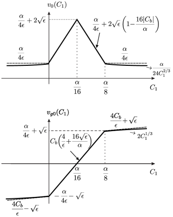
Figure 7: Dependence of position of the lower tip of the current-carrying triangle on the curvature. Black thick lines are dependencies of $v_{0}$ (top panel) and $v_{g0}$ (bottom panel) on $C_{1}$ for weak disorder and weak electro-mechanical coupling $\alpha$ ($C_{1}{\ll}\epsilon^{3/2},$ $\alpha{\ll}\epsilon^{3/2}$). At larger $C_{1}$ ($|C_{1}|{\gg}\epsilon^{3/2}$), $v_{0}$ starts to decrease very slowly, ${\sim}\alpha/C_{1}^{2/3},$ while linear increase of $v_{g0}$ with $C_{1}$ slows down to ${\sim}C_{1}^{1/3}.$ Dashed lines show asymptotical behavior of $v_{0}$ and $v_{g0}$ for $C_{1}\ll\epsilon^{3/2}.$ Thick curves deviate significantly from dashed ones for $|C_{1}|\sim\epsilon^{3/2}\gg\alpha.$

IV.4 Limiting cases

Next, we consider some limiting cases. General equations derived in the previous section are dramatically simplified when $C_{1}$ and $\alpha$ are small:

$$C_{1}\ll\epsilon^{3/2},\quad\alpha\ll\epsilon^{3/2}.$$ (36)

Then, keeping in $\theta^{\pm}_{s}$ terms up to linear order with respect to $C_{1}$ and $\alpha,$ and in $\omega_{s}^{\pm}$ up to quadratic order we get

$$\theta_{s}^{\pm}\approx\pm\sqrt{\epsilon}+\frac{4C_{s}}{\epsilon},$$ (37)

$$\omega_{s}^{\pm}\approx-\frac{16C_{s}^{2}}{\epsilon}\mp 8C_{s}\sqrt{\epsilon}.$$ (38)

Substituting Eq. (38) into Eqs. (33) and (34) we find that the latter equations can be written in a compact way (it is convenient to express $v_{0}$ and $v_{g0}$ in terms of $C_{b}$:

$$v_{0}(C_{1}){=}\begin{cases}\displaystyle\frac{\alpha}{4\epsilon},&\displaystyle\text{for}~{}|C_{b}|{>}\frac{\alpha}{16}\\ \displaystyle\frac{\alpha}{4\epsilon}+2\sqrt{\epsilon}\left(1{-}\frac{16|C_{b}|}{\alpha}\right),&\displaystyle\text{for}~{}|C_{b}|{<}\frac{\alpha}{16},\end{cases}$$ (39)

$$v_{g0}(C_{1}){=}\begin{cases}\displaystyle\frac{4C_{b}}{\epsilon}{+}{\rm sign}(C_{b})\sqrt{\epsilon},&\displaystyle\text{for}~{}|C_{b}|{>}\frac{\alpha}{16}\\ \displaystyle C_{b}\left(\frac{4}{\epsilon}{+}\frac{16\sqrt{\epsilon}}{\alpha}\right),&\displaystyle\text{for}~{}|C_{b}|{<}\frac{\alpha}{16}.\end{cases}$$ (40)

Dependencies of $v_{0}$ and $v_{g0}$ on $C_{1}$ are schematically shown in Fig. 7. Most interestingly, there is a very sharp increase of $v_{0}$ (and, consequently, $v_{\rm Th}$) within a narrow region of disorder strength: $0{<}C_{1}{<}\alpha/8.$ Hence, we predict the suppression of the current by the built-in curvature— the phenomenon, which we call elastic curvature blockade. Physically, curvature-induced threshold in the current arises due to the need to choose the bending amplitude $\theta_{1}$ from minimization of $W(\theta_{1})$. For $|v|{<}v_{\rm Th}$, the bending angle found from energy minimization (with account of the electro-mechanical coupling) turns out to be beyond the current-carrying window $v_{-}{<}\theta_{1}{<}v_{+}.$

One can also find dependence of $v_{0}$ on $\epsilon.$ The results of corresponding numerical solution is shown in Fig. 8. As one can see, this dependence is very sensitive to a built-in curvature. In particular, the change of $C_{1}$ from negative to positive values results in qualitative change of the behavior of $v_{\rm 0}$ with $\epsilon$.

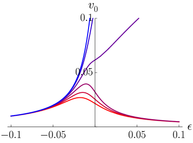
Figure 8: Dependence of the elastic-blockade-induced voltage, $v_{0}$, on $\epsilon$ for $\alpha{=}2\cdot 10^{-3}$ at different values of $C_{1}$ ranging from $-1.25\cdot 10^{-4}$ to $1.25\cdot 10^{-4}$ (from red to blue) with the step $0.5\cdot 10^{-4}$. For $\epsilon{>}0,$ the built-in curvature enhances parametrically the voltage $v_{0}.$

Equations (39) and (40) can be further simplify in the absence of disorder, $C_{1}{=}0.$ In this case, $v_{0}{=}\alpha/4\epsilon$ $v_{g0}{=}{-}\sqrt{\epsilon}{-}\alpha/4\epsilon,$ so we obtain

$$v_{\rm Th}=\frac{\alpha}{4\epsilon}+2\left|v_{g}+\sqrt{\epsilon}+\frac{\alpha}{4\epsilon}\right|,\quad{\rm for}~{}C_{1}=0.$$ (41)

This result is in agreement with Refs. [16, 17, 18], where it was found that electro-mechanical coupling leads to elastic blockade. Indeed, we see that there is a finite minimal threshold voltage, $v_{\rm Th}^{\rm min}={\alpha}/{4\epsilon},$ proportional to electro-mechanical coupling. This means that at low temperatures and small driving voltage, the transport through SET is blocked.

In the limit of very small $\alpha,$ one can easily get $I-V$ curve for arbitrary values of $C_{1}.$ To this end, one should take limit $\alpha{\to}0$ in Eqs. (33), and (34). Simple calculation yields $v_{0}{\to}0$ and $v_{g0}{\to}\theta_{1}(C_{1})$ where $\theta_{1}(C_{1})$ is given by Eq. (22). Therefore, we get

$$v_{\rm Th}=2\left|v_{g}-\theta_{1}(C_{1})\right|,\quad{\rm for}\quad\alpha\to 0.$$ (42)

Since $\theta_{1}(C_{1})$ has a jump at $C_{1}{=}0$ (see Fig. 4), current-carrying triangle also abruptly “jumps” in $v_{g}$ direction on $\delta v_{g}{=}2\sqrt{\epsilon},$ when $C_{1}$ changes sign. Exactly at the point $v_{g}{=}0$ and for $|C_{1}|{\ll}\epsilon^{3/2},$ we get $v_{\rm Th}{\approx}2\sqrt{\epsilon}.$ Comparing this value with the value $\alpha/4\epsilon$ for finite $\alpha$ and $C_{1}{\equiv}0$ [see Eq. (41)], we find giant, about $\epsilon^{3/2}\alpha^{-1}{\gg}1,$ curvature-induced enhancement of the driving voltage threshold, as compared to the elastic blockade threshold, in the absence of the curvature [16, 17, 18].

Before closing this section, we note that Eqs. (39) and (40) have finite limit when both $C_{1}$ and $\alpha$ tends to zero, while the ratio $C_{1}/\alpha{=}(1+\xi)/16$ remains finite. Then, we find

$$\frac{v_{0}}{2\sqrt{\epsilon}}=\left\{\begin{array}[]{ll}1-|\xi|,&\quad{\rm for}~{}|\xi|<1,\\ 0,&\quad{\rm for}~{}|\xi|>1,\end{array}\right.$$ (43)

$$\frac{v_{g0}}{\sqrt{\epsilon}}=\left\{\begin{array}[]{ll}\xi,&\quad{\rm for}~{}|\xi|<1,\\ {\rm sign}[\xi],&\quad{\rm for}~{}|\xi|>1.\end{array}\right.$$

Physically, approximation (43) neglects relatively small effects caused by elastic blockade in the absence of curvature, but captures much larger curvature-induced blockade. Within this approximation, position of the current-carrying triangle is fully determined by parameter $\xi=16C_{\rm b}/\alpha{=}16C_{\rm 1}/\alpha{-}1.$ With increasing $\xi$ from ${-}\infty$ to $\infty$ the lower tip of the triangle moves in the following way: it remains stationary in the position $(v_{g0}{=}{-}\sqrt{\epsilon},v_{0}{=}0)$ for ${-}\infty{<}\xi{<}{-}1,$ then “climbs a hill” with a height $2\sqrt{\epsilon}$ in the interval ${-}1{<}\xi{<}0,$ moves down in the interval $0{<}\xi{<}1,$ and finally arrives at the position $(v_{g0}{=}\sqrt{\epsilon},v_{0}{=}0)$ and remains stationary for $1{<}\xi{<}\infty.$ This approximation neglects very slow motion of the triangle at large $|\xi|{>}1$ (see the bottom panel in Fig. 7). The change of $v_{g0}$ from ${-}\sqrt{\epsilon}$ to $\sqrt{\epsilon}$ with increasing $\xi$ is due to curvature-induced re-buckling of the nanotube.

V Disorder-averaged $I-V$ curve

Next we assume that a random $C_{1}$ is described by a distribution function $\mathcal{P}(C_{1}).$ Changing $C_{1}$ in the interval, ${-}\infty{<}C_{1}{<}\infty,$ one can find the curve $(v_{g}(C_{1}),v_{0}(C_{1}))$ in $(v_{g},v)$ plane parameterized by $C_{1}.$ This curve yields limiting value $\overline{v}_{\rm Th}(v_{g}),$ below which the current is equal to zero for any $C_{1}$ and consequently, for disorder-averaged $I-V$ curve. Using general properties of functions $v_{0}(C_{1})$ and $v_{g0}(C_{1})$ [see discussion after Eq. (35)], one can easily find that $\overline{v}_{\rm Th}(v_{g})$ has a maximum at $v_{g}{=}0$ and is symmetric with respect to this point: $\overline{v}_{\rm Th}(v_{g}){=}\overline{v}_{\rm Th}({-}v_{g}).$ Dependence $\overline{v}_{\rm Th}(v_{g})$ is shown schematically in Fig. 9. For small $\alpha$ obeying inequality (36), this dependence reads

$$\overline{v}_{\rm Th}(v_{g})=\begin{cases}\displaystyle\frac{\alpha}{4\epsilon},&\text{for}~{}|v_{g}|{>}\overline{v}_{g},\\ \displaystyle 2\sqrt{\epsilon}\left(1{+}\frac{\alpha}{8\epsilon^{3/2}}\right){-}\frac{2|v_{g}|}{1{+}\frac{\alpha}{4\epsilon^{3/2}}},&\text{for}~{}|v_{g}|{\leqslant}\overline{v}_{g},\end{cases}$$ (44)

where $\overline{v}_{g}{=}\sqrt{\epsilon}[1{+}\alpha/(4\epsilon^{3/2})]$.

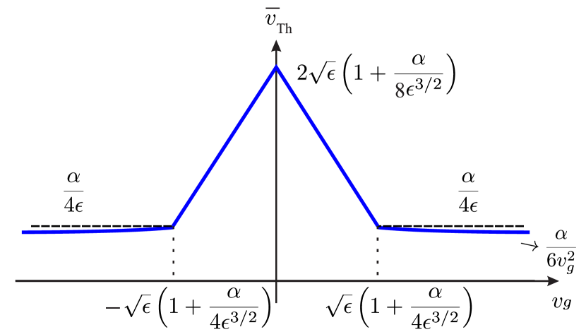
Figure 9: Dependence of the threshold voltage, $\overline{v}_{\rm Th}$ on $v_{g}.$ Below the curve $\overline{v}_{\rm Th}(v_{g})$ disorder-averaged current equals to zero. For $0<|v_{g}|-\sqrt{\epsilon}\ll\sqrt{\epsilon},$ the thershold voltage is approximately constant and given by $\alpha/4\epsilon$ (dashed line).

One can also show that for very large gate voltages, $v_{g}{\gg}\sqrt{\epsilon},$ the threshold voltage decays as $\overline{v}_{\rm Th}(v_{g}){\approx}\alpha/(6v_{g}^{2}).$

We stress that $\overline{v}_{\rm Th}(v_{g})$ does not depend on the distribution function of the random curvature, $\mathcal{P}(C_{1}),$ provided that this function is non-zero within the whole interval $-\infty{<}C_{1}{<}\infty.$ To be specific, we assume that the random curvature has Gaussian distribution with the zero mean and

$$\langle C^{\prime}(s_{1})C^{\prime}(s_{2})\rangle=\Delta\delta(s_{1}-s_{2}),$$ (45)

where $C^{\prime}(s){=}dC(s)/ds.$ Then the eigenmodes $C_{n}$ are independently correlated with the dispersion determined by $\Delta$,

$$\left\langle C_{n}C_{m}\right\rangle=\Delta_{n}\delta_{nm},\quad\Delta_{n}=\frac{2\Delta L}{\pi^{2}n^{2}},\quad n=1,2,\dots.$$ (46)

Hence, $C_{1}$ has the normal distribution,

$$\mathcal{P}(C_{1})=\frac{\exp\left(-{C_{1}^{2}}/{2\Delta_{1}}\right)}{\sqrt{2\pi\Delta_{1}}},$$ (47)

characterized by the variance $\Delta_{1}.$

The point $\{v_{\rm g0}(C_{1}),v_{0}(C_{1})\}$ is the position of the lower tip of triangle region of non-zero current. This point moves as $C_{1}$ is increasing from negative to positive values. As shown in Fig. 2, for $v{>}\overline{v}_{\rm Th}(v_{g}),$ there are two values of curvature $C_{\rm R}$ and $C_{\rm L}$ ($C_{\rm L}{>}C_{\rm R}$) for which, respectively, right and left boundaries of the current-carrying triangle cross a point $(v_{g},v).$ Since at any point belonging to the triangle the current equals $I=1/2,$ and equals to zero outside the triangle, we get the following expressions for averaged current and the current distribution function

$$\langle I\rangle{=}\frac{1}{2}\int\limits_{C_{\rm R}}^{C_{\rm L}}dC_{1}\mathcal{P}(C_{1}){=}\frac{1}{2}\left[\mathop{\rm erf}\left(\frac{C_{\rm L}}{\sqrt{2\Delta_{1}}}\right){-}\mathop{\rm erf}\left(\frac{C_{\rm R}}{\sqrt{2\Delta_{1}}}\right)\right],$$

$$\mathcal{P}_{\rm cur}(I)=2\langle I\rangle\delta(I-1/2)+(1-2\langle I\rangle)\delta(I).$$ (48)

As follows from Eqs. (32), $C_{\rm R,L}$ are implicitly defined by the following equations:

$$v_{-}=v_{g0}(C_{\rm R})-\frac{v_{0}(C_{\rm R})}{2},\quad v_{+}=v_{g0}(C_{\rm L})+\frac{v_{0}(C_{\rm L})}{2}.$$ (49)

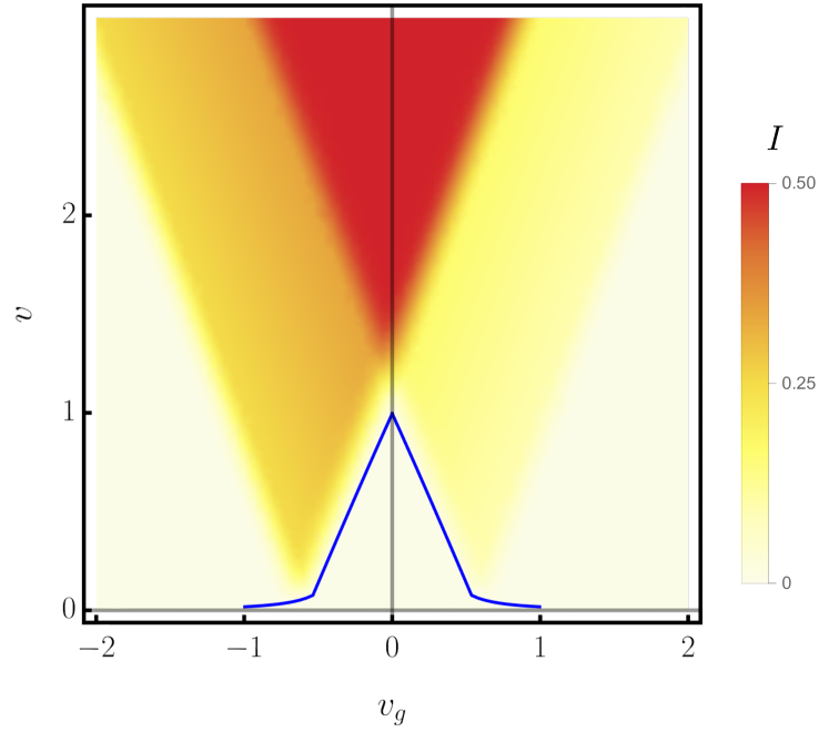
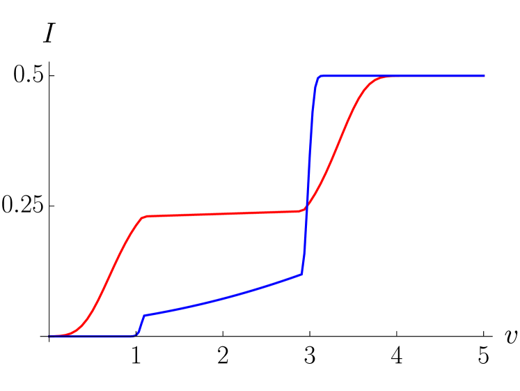
Figure 10: Top panel: Density plot of the averaged current for $\epsilon{=}0.2$, $\alpha{=}0.1$, and $\Delta_{1}{=}2\cdot 10^{-4}.$ The blue solid curve is the threshold $\overline{v}_{\rm Th}(v_{\rm g})$. Bottom panel: The current-voltage characteristics for $v_{\rm g}{=}1,$ $\alpha{=}0.02$ and different values of disorder variance $\Delta_{1}{=}8\cdot 10^{-4}$ and $\Delta_{1}{=}3\cdot 10^{-6}$ (red and blue correspondingly) for zero temperature. As seen, with increasing $\Delta_{1}$ an intermediate plateau appears corresponding to $I=1/4.$

Here functions $v_{0}(C)$ and $v_{g0}(C)$ are determined by Eqs. (28), (30), (33), and (34). Equation (48) suggests that $\langle I\rangle$ cannot exceed the value $1/2$.

The density plot of the average current calculated numerically with the use of Eq. (48) as the function of $v$ and $v_{\rm g}$ is shown in the top panel of Fig. 10. Numerically calculated current-voltage curve is presented in the bottom panel of Fig. 10 for two different values of variance $\Delta_{1}.$ One can also obtain analytical solution for $I-V$ by using approximation (43). Corresponding calculations are delegated to Appendix B.

Analysis of the numerical and analytical solutions demonstrate that at fixed $v_{\rm g}$, the value $1/2$ for the current is reached at large values of $v$ when $C_{\rm L}{\to}\infty,~{}C_{\rm R}{\to}{-}\infty$. One of the most interesting properties of the averaged $I-V$ curve is appearance of an intermediate plateau at $I{=}1/4$ with increasing disorder variance. This property is illustrated in the bottom panel of Fig. 10 and in Fig. 16. In order to understand physics behind this phenomenon, we will discuss in the next section the distribution function of the angle $\theta_{1}.$

VI The distribution function of the bending angle, $\theta_{1}$

The probability distribution function (PDF) for the bending angle $\theta_{1}$ is given by

$$P(\theta_{1})=\bigl{\langle}\delta[\theta_{1}-\theta_{1}(C_{1})]\bigr{\rangle}_{C_{1}},$$ (50)

where function $\theta_{1}(C_{1})$ gives solution of equation $f(\theta_{1})=0,$ corresponding to the global minimum of $W$ and angular brackets stand for the averaging with function $\mathcal{P}(C_{1})$ [see Eq. (47)]. Average current can be found (instead of integration over $C_{1},$ according to Eq. (48)) with the use of $P(\theta_{1})$ by integration within the current-carrying window:

$$\langle I\rangle=\int\limits_{v_{-}}^{v_{+}}P(\theta_{1})d\theta_{1}.$$ (51)

VI.1 Distribution of the bending angle in the absence of electro-mechanical coupling

Let us first consider the case of zero electro-mechanical coupling. For $\alpha{=}0,$ $\theta_{1}(C_{1})$ is shown in Fig. 4 and for $\epsilon{>}0$ is expressed in terms of $\theta^{\pm}(C)$ according to Eq. (24).

Integration of the delta functions in Eq. (50) over $C_{1}$ yields

$$P(\theta_{1})=\frac{1}{\sqrt{2\pi\Delta_{1}}}\left[\frac{d\theta_{1}(C_{1})}{dC_{1}}\right]^{-1}e^{-[C_{1}(\theta_{1})]^{2}/(2\Delta_{1})}$$ (52)

$$=\frac{(3\theta_{1}^{2}-\epsilon)~{}\Theta(\theta_{1}^{2}-\epsilon)}{8\sqrt{2\pi\Delta_{1}}}\exp\left[-\frac{(\theta_{1}^{3}-\epsilon\theta_{1})^{2}}{128\Delta_{1}}\right].$$ (53)

Here, we took into account that $C_{1}{=}C_{1}(\theta_{1})$ is given by Eq. (22) and used the following equation

$$J(\theta_{1})=\frac{dC_{1}(\theta_{1})}{d\theta_{1}}=\frac{3\theta_{1}^{2}-\epsilon}{8}$$ (54)

for the Jacobian (we write here $J(\theta_{1})$ instead of $|J(\theta_{1})|$, since $J(\theta_{1}){>}0$ in the region $|\theta_{1}|{>}\sqrt{\epsilon}$ where $P(\theta_{1}){>}0$.). The $\Theta$-function entering Eq. (53) reflects opening a gap in the distribution function.

In the limit of a very weak disorder, the distribution function consists of two delta peaks,

$$P(\theta_{1})\big{|}_{\Delta_{1}\to 0}=\frac{1}{2}\Bigl{[}\delta(\theta_{1}-\Delta_{\epsilon})+\delta(\theta_{1}+\Delta_{\epsilon})\Bigr{]}.$$ (55)

Here $\Delta_{\epsilon}{=}\sqrt{\epsilon}~{}\Theta(\epsilon)$ is the buckling-induced gap. The disorder broadens the delta functions in Eq. (55).

The function $P(\theta_{1})$, described by Eq. (53), is plotted in Fig. 11. for a fixed weak disorder and two values of $\epsilon,$ below and above instability threshold. Above the threshold, $\epsilon{>}0$, there is a gap $|\theta_{1}|{<}\Delta_{\epsilon}$ inside which $P(\theta_{1}){\equiv}0$. We also notice that slightly above the gap the distribution function increases despite of the presence of the damping exponent in Eq. (53). This increase is due to the Jacobian, $J(\theta_{1}).$

Although the terms involving higher curvature harmonics $C_{n>1}$ are small, they can modify the result (53) in the region where $P(\theta_{1})$ is very small. In particular, they lead to appearance of tails inside the gap, $|\theta_{1}|{<}\Delta_{\epsilon}$, for $\epsilon{>}0$ and to some modification of $P(\theta_{1})$ for $\epsilon{<}0$. We discuss in detail the effects of the higher harmonics in Appendix A and demonstrate that these modifications do not lead to significant change of the distribution function. In particular, as one can see from Fig. 14, even in the case of a moderate disorder, when delta peaks in the distribution function at $\theta_{1}{=}\Delta_{\epsilon}$ are essentially broadened, the smearing of the gap edges is quite small. Therefore, we shall neglect the corrections due to the high-order harmonics to $P(\theta_{1})$ in the rest of the paper.

VI.2 Effect of the electro-mechanical coupling

As we demonstrated above, equation $f(\theta_{1}){=}0$ has several solutions belonging to the manifold $\theta_{s}^{\pm}(C_{1})$ (see Fig. 5). These solutions and corresponding energies depend on $C_{1}.$ Since function $f(\theta_{1})$ has jumps at points $\theta_{1}{=}v_{-}$ and $\theta_{1}{=}v_{+},$ the function $\theta_{1}(C_{1}),$ which, by definition, represents the solution with the minimal energy, might have mini-jumps in addition to a large jump existing in the case $\alpha{=}0.$ Existence of these mini-jumps as well as their positions and position of the large jump depend on $v_{g},v,$ and on the value of $\alpha.$ For illustration, in Fig. 12 we plotted $\theta_{1}(C_{1})$ and corresponding distribution function,

$${P}(\theta_{1})=\bigl{[}{d\theta_{1}(C_{1})}/{dC_{1}}\bigr{]}^{-1}\mathcal{P}(C_{1})\Bigl{|}_{C_{1}=C_{1}(\theta_{1})}$$ (56)

(here $C_{1}(\theta_{1})$ is the inverse function for $\theta_{1}(C_{1})$), for the case $v{>}\overline{v}_{\rm Th}(v_{g})$ and relatively large $v_{g}$ such that $C_{\rm R}{>}\alpha/8.$

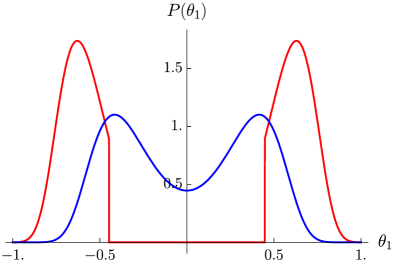
Figure 11: The distribution function for $\alpha{=}0,$ as determined by Eq. (53), for a fixed weak disorder, $\Delta_{1}{=}5\cdot 10^{-4}$, and for $\epsilon{=}\pm 0.2$ (red and blue curves, respectively)

As seen from this figure, there are three major effects of the electromechanical coupling: (i) the curve $\theta_{1}(C_{1})$ becomes asymmetric with respect to the inversion: $\theta_{1}\mapsto-\theta_{1};$ (ii) several vertical mini-jumps form on this dependence in addition to the large jump; (iii) large jump between values of the bending angle close to $-\sqrt{\epsilon}$ and $\sqrt{\epsilon}$ shifts from $C_{1}{=}0$ to the point $C_{1}{=}\alpha/8$ (this specific value depends on a position of point in the $(v_{g},v)$ plane).

Let us discuss these properties in more detail. First, we notice that $W^{+}_{s}{-}W^{-}_{s}$ change sign when $C_{s}{=}0$ (in particular, for $|C_{s}|{\ll}\epsilon^{3/2},$ we get $W^{+}_{s}{-}W^{-}_{s}{\approx}{-}16C_{s}\sqrt{\epsilon}$). Since, by assumption, $C_{\rm R}{>}\alpha/8,$ large jump occurs with increasing $C_{1}$ at the point $C_{a}{=}0,$ i.e. at $C_{1}{=}\alpha/8,$ where $W^{+}_{a}{=}W^{-}_{a}$ and, consequently, there happens a jump from $\theta_{a}^{-}$ to $\theta_{a}^{+}.$ With further increase of $C_{1}$ it reach the value $C_{1}{=}C_{\rm R},$ where solution jump into current-carrying triangle $\theta_{a}^{+}{\to}\theta_{b}^{+},$ and further jumps out the triangle, $\theta_{b}^{+}{\to}\theta_{c}^{+}$ at $C_{1}{=}C_{\rm L}.$ The values of $C_{\rm L,R}$ can be found from Eqs. (39), (40) and (49):

$$C_{\rm R}{\approx}\frac{3\alpha}{32}{+}\frac{\epsilon}{4}\left(v_{-}{-}\sqrt{\epsilon}\right),\quad C_{\rm L}{\approx}\frac{\alpha}{32}{+}\frac{\epsilon}{4}\left(v_{+}{+}\sqrt{\epsilon}\right).$$ (57)

The averaged current is given by Eq. (48), while the amplitudes of jumps read: $\delta\theta_{\rm R}=\theta_{b}^{+}(C_{\rm R})-\theta_{a}^{+}(C_{\rm R}),$ $\delta\theta_{\rm L}=\theta_{c}^{+}(C_{\rm L})-\theta_{b}^{+}(C_{\rm L}).$ For small $\alpha,$ obeying Eq. (36), we obtain

$$\delta\theta_{\rm R}\approx\delta\theta_{\rm L}\approx\frac{\alpha}{4\epsilon}.$$ (58)

As seen from Fig. 12, probability that the bending angle is close to the value ${-}\sqrt{\epsilon}$ is larger than the probability that $\theta_{1}{\approx}\sqrt{\epsilon}.$ The probability imbalance increases with decreasing $\Delta_{1}.$ For $\sqrt{\Delta}_{1}{\ll}\alpha,$ the bending angle with exponential precision is concentrated near ${-}\sqrt{\epsilon}.$

       

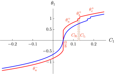
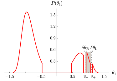
Figure 12: Left: Dependence of $\theta_{1}$ corresponding to the absolute minimum of the energy, on disorder strength $C_{1}$ for $\epsilon{=}{\pm}0.2$ (red and blue) and $\alpha{=}0.4,\;v_{g}{=}1,\;v{=}0.2.$ Dependence consists of several parts described by functions $\theta_{a}^{-}(C_{1}),~{}\theta_{a}^{+}(C_{1}),~{}\theta_{b}^{+}(C_{1}),$ and $\theta_{c}^{+}(C_{1}).$ Large jump occurs at $C_{1}{=}\alpha/8,$ while two small mini-jumps occur at the values $C_{1}{=}C_{\rm R}$ and $C_{1}{=}C_{\rm L},$ corresponding to the intersection of the point $(v_{g},v).$ by the right and left boundaries of current carrying triangle, respectively. Right: Bending angle distribution function for the curvature variance $\Delta_{1}{=}5\cdot 10^{-3}$ and $\epsilon{=}0.2$. Grey area in both panels corresponds to non-zero current. Voltages $v_{-}$ and $v_{+}$ are situated in the centers of mini-gaps.

Let us now discuss the physics behind the additional random-curvature-induced plateau in the $I-V$ curve. The key point is the competition between two symmetry breaking mechanisms: electro-mechanical coupling and random curvature. Remarkably, the limits $\alpha{\to}0$ and $\Delta_{1}{\to}0$ do not commute. Indeed, for $\alpha{\equiv}0$ and variance tending to zero, $\Delta_{1}{\to}0,$ energy $W(\theta_{1})$ has two degenerate minima for $\epsilon{>}0$. Thus, distribution function is given by the sum of two delta-functions:

$$P_{\Delta}={P}(\theta_{1})_{\Delta_{1}{\to}0,\alpha{=}0}{\simeq}\frac{1}{2}\left[\delta(\theta_{1}{+}\sqrt{\epsilon})+\delta(\theta_{1}{-}\sqrt{\epsilon})\right].$$

Although a weak disorder slightly broadens the delta functions, the symmetry ${P}_{\Delta}(\theta_{1}){=}{P}_{\Delta}({-}\theta_{1})$ remains intact. In the considered limit, $\Delta_{1}{\to}0$ and $\alpha{=}0$, expression for average current reads

$$\langle I\rangle{=}\frac{1}{2}\int\limits_{v_{-}}^{v_{+}}P_{\Delta}(\theta_{1})d\theta_{1}.$$

One can easily check that this expression contains an intermediate plateau with $\langle I\rangle=1/4$ in a wide interval of $v$ in addition to the plateau with $\langle I\rangle=1/2$ for $v\to\infty.$ By contrast, setting $\Delta_{1}{=}0$ first and, then, sending $\alpha{\to}0$, we find asymmetrical distribution function,

$$P_{\alpha}={P}_{\Delta_{1}{=}0,\alpha{\to}0}(\theta_{1})=\delta(\theta_{1}{+}\sqrt{\epsilon}).$$

Corresponding expression for the average current,

$$\langle I\rangle{=}\frac{1}{2}\int\limits_{v_{-}}^{v_{+}}P_{\alpha}(\theta_{1})d\theta_{1},$$

has only a single plateau with $\langle I\rangle=1/2$ for $v\to\infty.$ The competition between two mechanisms is controlled by the parameter $\sqrt{\Delta_{1}}/\alpha$ (see also Appendix B). An additional step in the $I-V$ curve appears when this parameter becomes large: $\sqrt{\Delta_{1}}/\alpha\gg 1.$ Remarkably, the current can be enhanced by disorder contrary to naive expectations (see the bottom panels in Fig. 10 and Fig. 16b).

VII Discussions and conclusions

In this paper, we predict curvature-induced enhancement of elastic blockade. The maximal position of the tip of the current-carrying triangle is given by $eV_{0}^{\rm max}{=}(a_{1}EL/\pi)v_{0}(C_{b}=0)$ [see Eqs. (15) and (39)]. Hence,

$$eV_{0}^{\rm max}\sim eEL\sqrt{\epsilon}.$$ (59)

For $E{\simeq}10$ kV/cm, $L{\simeq}0.1\,\mu$m and $\epsilon{\sim}1$ it gives $eV_{0}^{\rm max}{\sim}0.1$ eV that is larger than the charging energy $E_{\rm c}{\sim}10$ meV. We note that enhanced bias-voltage threshold of the order of $eV_{0}^{\rm max}$ exists for a sufficiently weak built-in curvature, in a narrow window, $0{<}C_{1}{<}\alpha/8$. Away from this window the bias-voltage threshold is parametrically reduced (for $\alpha{\ll}\epsilon^{3/2}$) and becomes of the order of the threshold in the clean case [16, 17, 18]. From Eq. (41), we find $v_{0}^{\rm cl}{=}\alpha/4\epsilon,$ so that

$$eV_{0}^{\rm cl}\sim\frac{\alpha}{\epsilon}eEL\ll eV_{0}^{\rm max}.$$ (60)

Eqs. (59) and (60) imply that bias threshold voltage very sharply depends on disorder: it changes by a large factor $\epsilon^{3/2}/\alpha$ in a very narrow region of small $C_{1}.$ For the experiments of Ref. [46] we can roughly estimate absolute value of curvature $|C_{1}|\lesssim 0.1{\div}1.$ For this estimate we used Eq. (9) with $F{=}0$ (i.e. $\epsilon{=}{-}8$) and values of $\theta_{1}^{\rm built-in}$ estimated from images of bent nanotubes in Ref. [46]. We also assumed that in equilibrium $C_{1}{\sim}\theta_{1}^{\rm built-in}$ (this estimate follows from Eq. (5) for $F{=}0$ and small $\alpha$). Although the microscopic model of built-in curvature is absent so far, one may expect that disorder-induced bending angle is not very sensitive to length of the nanotube. Due to smallness of $\alpha,$ the above estimates imply that built-in curvature might dominate electron transport through a nanotube-based SET for typical values of experimental parameters. It is worth noting that the threshold voltage given by Eq. (59) does not depend on the curvature but increases with length. Therefore, for long nanotubes used in Ref. [46], the effect of elastic blockade, which we discuss in the current work, is even higher and value $eV_{0}^{\rm max}$ is even larger compared to the estimate presented above. A more detailed comparison with experiment requires development of the microscopical theory of the elastic disorder, and therefore is out of scope of the current work devoted to development of the phenomenological approach.

In the previous sections we assumed that $T{=}0.$ Let us now discuss the effect of nonzero temperature. For a clean SET these effects were analyzed in Refs. [16, 17, 18]. The current depends on $T$ due to at least two reasons. At first, temperature enters the Fermi distribution functions in the expressions (6) and (7) for the average excess electron number and the current, respectively. Secondly, there are thermal fluctuations of the generalized coordinate $Y$, i.e. $\theta_{1}$. In the fundamental mode approximation these thermal fluctuations of the bending angle are described by the Gibbs factor $\exp[{-}\mathcal{E}_{\rm eff}(\theta_{1})/T]{=}\exp({-}W_{\rm eff}(\theta_{1})/\tilde{T})$ where $W_{\rm eff}(\theta_{1})$ and $\mathcal{E}_{\rm eff}(\theta_{1})$ are obtained from Eqs. (16) and (18) by replacement [see Eqs. (19) and (25) of Ref. [18]] $w_{d}{\to}w_{d,{\rm eff}}(\theta_{1}){=}({\tilde{T}}/{2})\sum_{\lambda{=}\pm}\ln\left[{f_{\rm F}(\alpha(v_{\lambda}{-}\theta_{1}))}/{f_{\rm F}(\alpha v_{\lambda})}\right]$. The effective dimensionless temperature is defined as

$$\tilde{T}=\frac{16LT}{\pi^{2}\kappa}.$$ (61)

As usual, a non-zero temperature results in smearing of the bias-voltage threshold in the current. For a fixed curvature $C_{1}$, our results for the current are valid provided temperature is much smaller than the threshold voltage,

$$T\ll eV_{0}(C_{1}).$$ (62)

Here voltage $V_{0}(C_{1}){=}(a_{1}/\pi)ELv_{0}(C_{1})$, cf. Eq. (32), is a very sharp function of curvature within the window $0{<}C_{1}{<}\alpha/8,$ changing within the interval $V_{0}^{\rm cl}{<}V_{0}(C_{1}){\leqslant}V_{0}^{\rm max}.$ As follows from the estimates presented above, $T$ is always smaller than $V_{0}^{\rm max}$ up to the room temperatures but can be much larger than $V_{0}^{\rm cl}$. Hence, the effect of temperature is negligible for $0{<}C_{1}{<}\alpha/8,$ but it can wash out the bias-voltage threshold for $C_{1}$ outside this interval.

In the case of a randomly distributed curvature the enhanced bias-voltage threshold (59) occurs near zero gate voltage, $V_{g}{\simeq}0$. Away from the elastic blockade peak the bias-voltage threshold is suppressed down to $V_{0}^{\rm cl}$, cf. Eq.(60). The thermal smearing is not important at temperatures $T{\ll}e\bar{V}_{\rm Th}(V_{g})$ where $\bar{V}_{\rm Th}(V_{g}){=}(a_{1}/\pi)EL\bar{v}_{\rm Th}(v_{g})$, cf. Eq. (44). For a random curvature distributed continuously, the average current is given as the average over $P(C_{1})$ and the Gibbs weight $\exp(-W_{\rm eff}(\theta_{1})/\tilde{T})$. The result of the corresponding numerical computation is shown on the Fig. 13. It illustrates blurring of the disorder-induced step in the $I-V$ curve at intermediate voltages by a finite temperature.

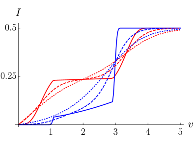
Figure 13: The current-voltage characteristics for $v_{\rm g}{=}1,$ $\alpha{=}0.02$ and different values of disorder variance $\Delta_{1}{=}8\cdot 10^{-4}$ and $\Delta_{1}{=}3\cdot 10^{-6}$ (red and blue correspondingly) for $\tilde{T}{=}0,\;2.5\cdot 10^{-3},\;5\cdot 10^{-3}$ (solid, dashed, dotted curves, respectively).

One of the most interesting problems to be solved in future is to study effect of disorder on high-quality resonances observed in Refs. [33, 34, 35, 36].

To summarize, we considered transport properties of a SET based on elastic nanotube with a regular or random built-in curvature in the strong Coulomb blockade regime. We demonstrated that close to the buckling transition, the $I$-$V$ curve of the transistor is extremely sensitive to such curvature.

Most importantly, we predict the following

• for fixed built-in curvature: a giant curvature-induced enhancement of the bias-voltage threshold (59) below which the current is exactly zero;

• for random curvature: the existence of an additional intermediate curvature-induced plateau in average $I-V$ curve, see Fig. 10.

Our predictions can be tested experimentally in systems similar to those studied in Refs. [33, 34, 35, 36].

Appendix A Effect of higher harmonics of the curvature

In this Appendix, we estimate effect of higher modes and demonstrate that this effect is small. We will focus on modification of the distribution function of $\theta_{1}$ caused by higher harmonics, neglecting electro-mechanical coupling. Generalization for the case $\alpha{\neq}0$ is straightforward but quite cumbersome and does not change our main conclusion about irrelevance of the higher order terms.

In order to find the equation for $\theta_{1},$ we perform an expansion of $\sin\theta$ to the third order, $\sin\theta{\approx}\theta{-}\theta^{3}/6$. Next, we use expansion (8) and, then, project the result onto the first harmonic, $n{=}1$. We keep terms up to the $\theta_{n}^{3}$. After some algebra, we arrive at the following cubic equation,

$$\theta_{1}^{3}-(\epsilon-\delta\epsilon)\theta_{1}+\theta_{1}^{2}\theta_{3}-8C_{1}=0,$$ (63)

where

$$\delta\epsilon=2\sum_{n=2}^{\infty}\theta_{n}\bigl{(}\theta_{n}+\theta_{n+2}\bigr{)}.$$ (64)

Here harmonics with $n{>}1$ for $|\epsilon|{\ll}1$ can be calculated within linear approximation, so we obtain

$$\theta_{n}\approx C_{n}\frac{q_{n}^{2}}{q_{n}^{2}-q_{1}^{2}},\quad\text{for}\quad n=2,3,\dots$$ (65)

They turn out to be finite at the instability threshold, $\epsilon{=}0.$ Consequently, the first harmonics dominate over higher-order ones. Hence, we can consider effect of higher harmonics perturbatively. As it follows from Eq. (65), the amplitudes $\theta_{n}$ with $n{\geqslant}2$ in Eqs. (63) and (64) are fixed by the disorder. Therefore, the problem is reduced to the analysis of the closed equation (63) for the most singular zero mode with the amplitude $\theta_{1}$. Just as in the case of single-mode approximation, for a fixed realization of disorder there are one or three real solutions of Eq. (63) for $\theta_{1}$.

Next, we discuss the effect of higher harmonics on the distribution function. We shall perform calculations in two steps. First, we average over fundamental harmonic $C_{1}$ for fixed $C_{n>1}.$ Next, we do averaging over higher harmonics. Let us introduce a new variable,

$$\theta_{1,{\rm eff}}=\theta_{1}+\frac{\theta_{3}}{3}=\theta_{1}+\frac{3C_{3}}{8}.$$ (66)

Here we used Eq. (65). Substituting Eq. (66) into Eq. (63), we get

$$\theta_{1,{\rm eff}}^{3}-\epsilon_{\rm eff}\theta_{1,{\rm eff}}=8\tilde{C}_{1},$$ (67)

where

$$\epsilon_{\rm eff}=\epsilon-\delta\epsilon+\frac{27}{64}C_{3}^{2},$$ (68)

$$\tilde{C}_{1}=C_{1}-\frac{1}{4}\left(\frac{3C_{3}}{8}\right)^{3}-\frac{3C_{3}}{64}(\epsilon-\delta\epsilon).$$

Equation (67) is equivalent to Eq. (22) up to a change of variables. Hence, by using calculations presented in the main text, we derive equation analogous to Eq. (53)

$$P(\theta_{1})=\exp\left[-\frac{(\theta_{1}^{3}-\epsilon\theta_{1})^{2}}{128\Delta_{1}}\right]\left\langle\frac{3\theta_{1}^{2}-\epsilon+\delta\epsilon+9\theta_{1}C_{3}/4}{8\sqrt{2\pi\Delta_{1}}}\right.$$

$$\times\left.\left[\Theta\left(\theta_{1}+\frac{3C_{3}}{8}-\Delta_{\epsilon_{\rm eff}}\right)\!+\!\Theta\left(-\theta_{1}-\frac{3C_{3}}{8}-\Delta_{\epsilon_{\rm eff}}\right)\right]\right\rangle$$ (69)

Here we calculated Jacobian by using Eq. (63). We also took into account that corrections due to high harmonics are small and can be fully neglected in the argument of the the exponent. The averaging in Eq. (69) is taken over $C_{n>1}.$

Further consideration depends on relation between $\Delta_{1}$ and $\epsilon.$ Below, we consider limits of both weak and strong disorder.

A.1 Weak disorder, $\Delta_{1}{\ll}|\epsilon|{\ll}1$

In this case, one can neglect disorder everywhere except the arguments of the step function, where we can also neglect the difference between $\epsilon_{\rm eff}$ and $\epsilon.$ Then disorder averaging is reduced to averaging of the step functions:

$$\left\langle\Theta\left(\!\!\pm\left[\theta_{1}+\frac{3C_{3}}{8}\right]-\Delta_{\epsilon}\right)\right\rangle_{C_{3}}\!\!\!\!\!=\frac{1}{2}{\rm erfc}\left[\frac{8(\Delta_{\epsilon}\mp\theta_{1})}{\sqrt{2\Delta_{1}}}\right].$$ (70)

Here we used $\Delta_{3}{=}\Delta_{1}/9$ (cf. Eq. (46)). The distribution function becomes

$$P(\theta_{1})=\frac{3\theta_{1}^{2}-\epsilon}{16\sqrt{2\pi\Delta_{1}}}\exp\left[-\frac{\left(\theta_{1}^{3}-\epsilon\theta_{1}\right)^{2}}{128\Delta_{1}}\right]$$ (71)

$$\times\left\{{\rm erfc}\left[\frac{8\left(\Delta_{\epsilon}-\theta_{1}\right)}{\sqrt{2\Delta_{1}}}\right]+{\rm erfc}\left[\frac{8\left(\Delta_{\epsilon}+\theta_{1}\right)}{\sqrt{2\Delta_{1}}}\right]\right\}.$$

Hence, for weak disorder, the only effect of the higher harmonics is blurring the step-like edge of the gap (for $\epsilon{>}0$) over a very narrow window $\delta\theta_{1}{\sim}\sqrt{\Delta}_{1}{\ll}\sqrt{\epsilon}.$

A.2 Strong disorder, $\epsilon{\ll}\Delta_{1}{\ll}1$

For strong disorder, one can neglect contribution of $\epsilon$ to $\epsilon_{\rm eff}.$ Then, $\epsilon_{\rm eff}{\approx}{-}\delta\epsilon{+}27C_{3}^{2}/64$. Then using the relation

$$2\sum\limits_{k=2}^{\infty}\left(\theta_{k}^{2}+\theta_{k}\theta_{k+2}\right)=\Bigl{[}\theta_{2}^{2}+(\theta_{2}+\theta_{4})^{2}+(\theta_{4}+\theta_{6})^{2}+\dots\Bigr{]}$$

$$+\Bigl{[}\theta_{3}^{2}+(\theta_{3}+\theta_{5})^{2}+(\theta_{5}+\theta_{7})^{2}+\dots\Bigr{]},$$ (72)

we prove that $\epsilon_{\rm eff}{<}0.$ Hence, $\Delta_{\epsilon_{\rm eff}}{=}0,$ so that the sum of two step functions in Eq. (69) equals to $1.$ Hence, we only need to average $\delta\epsilon$ in Eq. (69). Straightforward calculation yields

$$\big{\langle}\delta\epsilon\big{\rangle}_{C_{n>1}}=2\Delta_{1}\sum\limits_{n=2}^{n=\infty}\frac{n^{2}}{(n^{2}-1)^{2}}=\Delta_{1}\frac{3+4\pi^{2}}{24}.$$ (73)

Here, we used Eqs. (46) and (64). Substituting $\big{\langle}\delta\epsilon\big{\rangle}_{C_{n>1}}$ into Eq. (69), we obtain distribution function for $|\epsilon|{\ll}\Delta_{1}{\ll}1$:

$$P(\theta_{1})\!=\!\frac{3\theta_{1}^{2}\!+\!{(3+4\pi^{2})\Delta_{1}}/{24}}{8\sqrt{2\pi\Delta_{1}}}\exp\left[-\frac{\theta_{1}^{2}\left(\theta_{1}^{2}-\epsilon\right)^{2}}{128\Delta_{1}}\!\right].$$ (74)

A.3 Interpolation formula and gap formation

One can easily find a cross-over function that interpolates between weak and strong disorder limits. We note that both $\Delta_{1}$ and $\epsilon$ are still assumed to be smaller than unity. The cross-over function reads

$$P(\theta_{1}) \simeq\frac{3\theta_{1}^{2}-\epsilon+(3+4\pi^{2})\Delta_{1}/24}{16\sqrt{2\pi\Delta_{1}}}\exp\left[-\frac{\left(\theta_{1}^{3}-\epsilon\theta_{1}\right)^{2}}{128\Delta_{1}}\right]$$

$$\times\left[{\rm erfc}\left(\frac{8\left(\Delta_{\epsilon}-\theta_{1}\right)}{\sqrt{2\Delta_{1}}}\right)+{\rm erfc}\left(\frac{8\left(\Delta_{\epsilon}+\theta_{1}\right)}{\sqrt{2\Delta_{1}}}\right)\right].$$ (75)

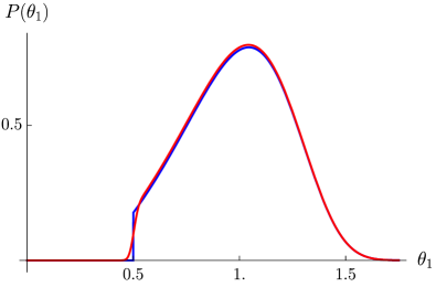
Figure 14: Distribution function calculated with the use of Eqs. (53) (blue) and (75) (red) for $\Delta_{1}{=}0.02$ and $\epsilon{=}0.25$.

Equation (75) describes formation of the gap in the distribution function. Due to coupling with higher harmonics, the edge of the gap is not infinitely sharp. Formally this is due to presence of $\rm ercf-$functions in Eq. (75) instead of $\Theta[\theta_{1}^{2}-\epsilon]$ in Eq. (53). Deep inside the gap, say for $\theta_{1}=0,$ perturbative expansion over harmonics fails and Eq. (75) becomes invalid. Correct calculation of exponentially small tails of the distribution function in the middle of the gap can be done by using optimal fluctuation method. Such calculation is out of scope of the current work. We also notice that comparison of Eqs.  (75) and (53) shown in Fig. 14 shows that difference between distribution functions calculated with and without account of high harmonics is quite small.

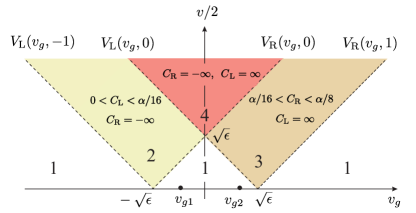
Figure 15: Phase diagram of the simplified model. The averaged current is equal to zero in the region $1$. It is equal to $1/2$ in the region $4.$ Dashed lines show positions of the right and left boundaries of the current-carrying triangle for $\xi{=}{-}1,0,1.$ Voltage-current curves for $v_{g}{=}v_{g1}$ and $v_{g}{=}v_{g2}$ are plotted in Fig. (16)

Appendix B Simplified model

Here, we discuss in more detail averaged current obtained within simplified model, when both $C_{1}$ and $\alpha$ tend to zero in such a way that the ratio $C_{1}/\alpha$ remains finite, cf. Eq. (43) and $\epsilon{>}0.$ Approximation (43) allows us to find exactly values of $C_{\rm L}$ and $C_{\rm R}$ entering Eq. (48), and, consequently, to find simple analytical equation for the curvature-averaged $I$-$V$ curve.

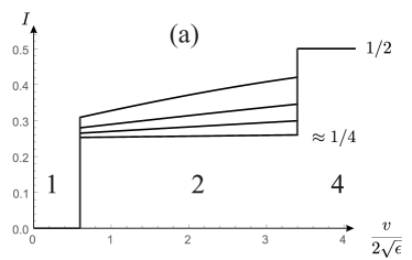
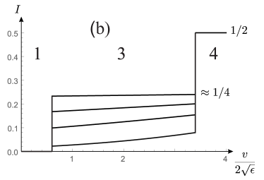
Figure 16: Voltage-current curves calculated within simplified model for two values $v_{g},$ corresponding to lines $v_{g}{=}v_{g1}{=}{-}0.7\sqrt{\epsilon}$ (a) and $v_{g}{=}v_{g2}{=}0.7\sqrt{\epsilon}$ (b) (see also Fig. 15) for $\alpha{=}0.016$ and different values of variance $\Delta_{1}$: $\sqrt{\Delta}_{1}{=}0.001,~{}0.002,~{}0.004,~{}0.2,$ which increases from bottom to top in panel (a) and from top to bottom in panel (b). In both cases, for large $\Delta_{1},$ an intermediate step with $I=1/4$ is formed.

Using Eq. (43), one can easily find how left and right boundaries of the current-carrying triangle move with changing $\xi$ in the interval $-1{<}\xi{<}1$:

$$v_{\rm L}(v_{g},\xi){=}2(\sqrt{\epsilon}-v_{g}){+}4\sqrt{\epsilon}~{}\xi\Theta\left(-\xi\right),$$ (76)

$$v_{\rm R}(v_{g},\xi){=}2(\sqrt{\epsilon}+v_{g}){-}4\sqrt{\epsilon}~{}\xi\Theta\left(\xi\right).$$ (77)

For $\xi{<}{-}1,$ the triangle does not move and is limited by lines $v_{\rm L}(v_{g},{-}1)$ and $v_{\rm R}(v_{g},0).$ For $\xi{>}1,$ the triangle is also stationary and is bounded by lines $v_{\rm L}(v_{g},0)$ and $v_{\rm R}(v_{g},1).$

We notice that in the interval ${-}1{<}\xi{<}0,$ the left boundary changes according to Eq. (76), while right boundary remains stationary and is still given by $v_{\rm R}(v_{g},0).$ For $0{<}\xi{<}1,$ left boundary stops and is given by $v_{\rm L}(v_{g},0),$ while right boundary starts to move according to Eq. (77). This is very similar to Fig. 2 with two minor distinctions: in the simplified model the boundaries of the current-carrying triangle are parallel to blue lines and we neglect slow motion of triangle for $C_{1}<0$ and $C_{1}>\alpha/8.$

Using Eqs. (49), (76) and (77) one can derive $C_{\rm L,R}$ in the regions $1,2,3,4$ of the phase diagram shown in Fig. 15. For any value of the curvature, points in the region $1$ are not covered by the current-carrying triangle, so that $C_{\rm L}=C_{\rm R}=\infty$ and $I\equiv 0.$ By contrast, all points of the region $4$ belong to the current-carrying cone for any $C_{1},$ hence, $I\equiv 1/2.$

For region $2$ we find $C_{\rm R}=-\infty,$ and

$$C_{\rm L}=\frac{\alpha}{64}\frac{v+2(\sqrt{\epsilon}+v_{g})}{\sqrt{\epsilon}},\qquad 0<C_{\rm L}<\frac{\alpha}{16}.$$ (78)

Here $C_{\rm L}$ is found from the condition $v{=}v_{\rm L}(v_{g},16C_{L}/\alpha{-}1).$ The averaged current in the region $2$ reads

$$I^{(2)}=\frac{1}{2}\int\limits_{-\infty}^{C_{\rm L}}P(C_{1})dC_{1}=\frac{1}{4}\left[1+{\rm erf}\left(\frac{C_{\rm L}}{\sqrt{2\Delta_{1}}}\right)\right].$$ (79)

In the region $3$ we get $C_{\rm L}=\infty$ and

$$C_{\rm R}=\frac{\alpha}{64}\frac{2(3\sqrt{\epsilon}+v_{g})-v}{\sqrt{\epsilon}},\qquad\frac{\alpha}{16}<C_{\rm R}<\frac{\alpha}{8}.$$ (80)

This result for $C_{\rm R}$ is derived from the condition $v{=}v_{\rm R}(v_{g},16C_{R}/\alpha{-}1).$ Averaged current in the region $3$ reads

$$I^{(3)}=\frac{1}{2}\int\limits^{\infty}_{C_{\rm R}}P(C_{1})dC_{1}=\frac{1}{4}{\rm erfc}\left(\frac{C_{\rm R}}{\sqrt{2\Delta_{1}}}\right).$$ (81)

Voltage-current curves calculated within simplified model for two values of the gate voltage $v_{g}{=}v_{g1}$ and $v_{g}{=}v_{g2}$ are shown in Fig. 16. The parameter $\alpha$ is kept fixed whereas the disorder strength varies. In both cases, for small driving voltage, in region $1,$ the current is equal to zero, while at very large $v,$ in region $4,$ the current is equal to $1/2.$ In the region $2$ (see Fig. 16a) the current is given by Eq. (79). In the region $3$ (see Fig. 16b) the current is given by Eq. (81). The main difference of the simplified model as compared to the exact one is the presence of sharp jumps between different regions of the $I-V$ curve. These jump are smoothed in a more accurate model (compare bottom panel of Fig. 10 and Fig. 16).

References

- [1] The special issue on single charge tunneling, Z. Phys. B 85, 317 (1991).
- [2] M. A. Kastner, The single-electron transistor, Rev. Mod. Phys. 64, 849 (1992).
- [3] Single Charge Tunneling, ed. by H. Grabert and M. H. Devoret (Plenum, New York, 1992)
- [4] W. G. van der Wiel, S. De Franceschi, J. M. Elzerman, T. Fujisawa, S. Tarucha, L. P. Kouwenhoven, Electron transport through double quantum dots, Rev. Mod. Phys. 75, 1 (2002).
- [5] R. Hanson, L. P. Kouwenhoven, J. R. Petta, S. Tarucha, L. M. K. Vandersypen, Spins in few-electron quantum dots, Rev. Mod. Phys. 79, 1217 (2007).
- [6] R. G. Knobel and A. N. Cleland, Piezoelectric displacement sensing with a single-electron transistor, Appl. Phys. Lett. 81, 2258 (2002).
- [7] R. G. Knobel and A. N. Cleland, Nanometre-scale displacement sensing using a single electron transistor, Nature (London) 424, 291 (2003).
- [8] N. Nishiguchi, Elastic deformation blockade in a single-electron transistor, Phys. Rev. B 68, 121305R (2003).
- [9] A. D. Armour, M. P. Blencowe, and K. C. Schwab, Entanglement and decoherence of a micromechanical resonator via coupling to a Cooper-pair box, Phys. Rev. Lett. 88, 148301 (2002).
- [10] L. Y. Gorelik, A. Isacsson, M. V. Voinova, B. Kasemo, R. I. Shekhter, and M. Jonson, Shuttle mechanism for charge transfer in coulomb blockade nanostructures, Phys. Rev. Lett. 80, 4526 (1998).
- [11] F. Pistolesi and R. Fazio, Charge shuttle as a nanomechanical rectifier, Phys. Rev. Lett. 94, 036806 (2005).
- [12] O. Usmani, Ya. M. Blanter, and Yu. V. Nazarov, Strong feedback and current noise in nanoelectromechanical systems, Phys. Rev. B 75, 195312 (2007).
- [13] A. G. Pogosov, M. V. Budantsev, A. A. Shevyrin, A. E. Plotnikov, A. K. Bakarov and A. I. Toropov, Blockade of tunneling in a suspended single-electron transistor, JETP Lett. 87, 150 (2008).
- [14] G. A. Steele, A. K. Hüttel, B. Witkamp, M. Poot, H. B. Meerwaldt, L. P. Kouwenhoven, and H. S. J. van der Zant, Strong coupling between single-electron tunneling and nanomechanical motion, Science 325, 1103 (2009).
- [15] B. Lassagne, Y. Tarakanov, J. Kinaret, D. Garcia-Sanchez, and A. Bachtold, Coupling mechanics to charge transport in carbon nanotube mechanical resonators, Science 325, 1107 (2009).
- [16] G. Weick, F. Pistolesi, E. Mariani, and F. von Oppen, Discontinuous Euler instability in nanoelectromechanical systems, Phys. Rev. B 81, 121409(R) (2010).
- [17] G. Weick, F. Von Oppen, and F. Pistolesi, Euler buckling instability and enhanced current blockade in suspended single-electron transistors, Phys. Rev. B 83, 035420 (2011).
- [18] G. Micchi, R. Avriller, and F. Pistolesi, Mechanical signatures of the current blockade instability in suspended carbon nanotubes, Phys. Rev. Lett. 115, 206802 (2015).
- [19] A. D. Armour, M. P. Blencowe, and Y. Zhang, Classical dynamics of a nanomechanical resonator coupled to a single-electron transistor, Phys. Rev. B 69, 125313 (2004).
- [20] J. Koch and F. von Oppen, Franck-Condon blockade and giant Fano factors in transport through single molecules, Phys. Rev. Lett. 94, 206804 (2005).
- [21] J. Koch, F. von Oppen, and A. V. Andreev, Theory of the Franck-Condon blockade regime, Phys. Rev. B 74, 205438 (2006).
- [22] D. Mozyrsky, M. B. Hastings, and I. Martin, Intermittent polaron dynamics: Born-Oppenheimer approximation out of equilibrium, Phys. Rev. B 73, 035104 (2006).
- [23] F. Pistolesi and S. Labarthe, Current blockade in classical single-electron nanomechanical resonator, Phys. Rev. B 76, 165317 (2007).
- [24] F. Pistolesi, Ya. M. Blanter, and I. Martin, Self-consistent theory of molecular switching, Phys. Rev. B 78, 085127 (2008).
- [25] R. Leturcq, C. Stampfer, K. Inderbitzin, L. Durrer, C. Hierold, E. Mariani, M. G. Schultz, F. von Oppen, and K. Ensslin, Franck–Condon blockade in suspended carbon nanotube quantum dots, Nat. Phys. 5, 327 (2009).
- [26] L. Euler, in Leonhard Euler’s Elastic Curves, translated and annotated by W. A. Oldfather, C. A. Ellis, and D. M. Brown, reprinted from ISIS, No. 58 XX(1), 1744 (Saint Catherine Press, Bruges).
- [27] L.D. Landau, E.M Lifshitz, Theory of elasticity; 2nd ed. Pergamon, Oxford (1970).
- [28] S. Sapmaz, Ya. M. Blanter, L. Gurevich, and H. S. J. van der Zant, Carbon nanotubes as nanoelectromechanical systems, Phys. Rev. B 67, 235414 (2003).
- [29] M. R. Falvo, G. J. Harris, R. M. Taylor II, V. Chi, F. P. Brooks Jr, S. Washburn, and R. Superfine, Bending and buckling of carbon nanotubes under large strain, Nature (London) 389, 582 (1997).
- [30] S. M. Carr and M. N. Wybourne, Elastic instability of nanomechanical beams , Appl. Phys. Lett. 82, 709 (2003).
- [31] S. M. Carr, W. E. Lawrence, and M. N. Wybourne, Buckling cascade of free-standing mesoscopic beams, Europhys. Lett. (EPL) 69, 952 (2005).
- [32] D. Roodenburg, J. W. Spronck, H. S. J. van der Zant, and W. J. Venstra, Buckling beam micromechanical memory with on-chip readout, Appl. Phys. Lett. 94, 183501 (2009).
- [33] S. L. de Bonis, C. Urgell, W. Yang, C. Samanta, A. Noury, J. Vergara-Cruz, Q. Dong, Y. Jin, and A. Bachtold, Ultrasensitive Displacement Noise Measurement of Carbon Nanotube Mechanical Resonators, Nano Lett. 18, 5324 (2018).
- [34] A. W. Barnard, M. Zhang, G. S. Wiederhecker, M. Lipson, P. L. McEuen, Real-time vibrations of a carbon nanotube, Nature 566, 89 (2019).
- [35] S. O. Erbil, U. Hatipoglu , C. Yanik, M. Ghavami, A. B. Ari, M. Yuksel, and M. S. Hanay, Full electrostatic control of nanomechanical buckling, Phys. Rev. Lett. 124, 046101 (2020).
- [36] X. Wang, L. Cong, D. Zhu, Z. Yuan, X. Lin, W. Zhao, Z. Bai, W. Liang, X. Sun, G.-W. Deng, and K. Jiang, Visualizing nonlinear resonance in nanomechanical systems via single-electron tunneling, Nano Research, 14 1156 (2021).
- [37] S. M. Carr, W. E. Lawrence, and M. N. Wybourne, Accessibility of quantum effects in mesomechanical systems, Phys. Rev. B 64, 220101(R) (2001).
- [38] P. Werner and W. Zwerger, Macroscopic quantum effects in nanomechanical systems, Europhys. Lett. (EPL) 65, 158 (2004).
- [39] V. Peano and M. Thorwart, Nonlinear response of a driven vibrating nanobeam in the quantum regime, New J. Phys. 8, 21 (2006).
- [40] S. Savel’ev, X. Hu, and F. Nori, Quantum electromechanics: qubits from buckling nanobars, New J. Phys. 8, 105 (2006).
- [41] P. Benetatos and E. M. Terentjev Stretching weakly bending filaments with spontaneous curvature in two dimensions, Phys. Rev. E 81, 031802 (2010).
- [42] P. Benetatos and E. M. Terentjev,Stretching semiflexible filaments with quenched disorder, Phys. Rev. E 82, 050802(R) (2010).
- [43] P. Benetatos and E. M. Terentjev, A constrained random-force model for weakly bending semiflexible polymers Phys. Rev. E 84, 022801 (2011).
- [44] C.-T. Lee, and E. M. Terentjev, Microtubule buckling in an elastic matrix with quenched disorder, J. Chem. Phys. 149, 145101 (2018).
- [45] We note that where denotes a similar dimensionless parameter used in Ref. [17].
- [46] Y. Fan, B. Goldsmith, and P. Collins, Identifying and counting point defects in carbon nanotubes, Nature Mater 4, 906 (2005).