Structured second-order methods via natural-gradient descent

Abstract

We propose new structured second-order methods and structured adaptive-gradient methods obtained by performing natural-gradient descent on structured parameter spaces. Natural-gradient descent is an attractive approach to design new algorithms in many settings such as gradient-free, adaptive-gradient, and second-order methods. Our structured methods not only enjoy a structural invariance but also admit a simple expression. Finally, we test the efficiency of our proposed methods on both deterministic non-convex problems and deep learning problems.

1 Introduction

Newton’s method is a powerful optimization method and is invariant to any invertible linear transformation. Unfortunately, it is computationally intensive due to the inverse of the Hessian computation. Moreover, it could perform poorly in non-convex settings since the Hessian matrix can be neither positive-definite nor invertible. To address these issues, structural extensions are proposed such as BFGS. However, these extensions often lose the linear invariance. Moreover, existing extensions are often limited to one kind of structures and may not perform well in stochastic settings.

In this paper, we introduce new efficient and structured 2nd-order updates that incorporate flexible structures and preserve a structural invariance. Unlike existing second-order methods, our methods can be readily used in non-convex and stochastic settings. Moreover, structured and efficient adaptive-gradient methods are easily obtained for deep leaning by using the Gauss-Newton approximation of the Hessian. This work is an extension and application of the structured natural-gradient method (Lin et al., 2021).

Many machine learning applications can be expressed as the following unconstrained optimization problem.

$$\min_{\mu\in\text{missing}^{p}}\ell(\mbox{$\mbox{$\boldsymbol{\mu}$}$})$$ (1)

where function $\ell$ is a loss function. Instead of directly solving (1), we consider to solve the following optimization problem over a probabilistic distribution $q$.

$$\min_{\boldsymbol{\tau}\in\Omega_{\tau}}\mathbb{E}_{\scaleto{q(\text{\mbox{$\mbox{$\mathbf{w}$}$}}|\boldsymbol{\tau})\mathstrut}{6pt}}\left[\ell(\mbox{$\mbox{$\mathbf{w}$}$})\right]-\gamma\mathcal{H}(q(\mbox{$\mbox{$\mathbf{w}$}$}|\boldsymbol{\tau}))$$

where $q(\mbox{$\mbox{$\mathbf{w}$}$}|\boldsymbol{\tau})$ is a parametric distribution with parameters $\boldsymbol{\tau}$ in the parameter space $\Omega_{\tau}$, $\mathcal{H}(q(\mbox{$\mbox{$\mathbf{w}$}$}))$ is Shannon’s entropy, and $\gamma\geq 0$ is a constant. Problem (1) arises in many settings such as gradient-free problems (Baba, 1981; Beyer, 2001; Spall, 2005), reinforcement learning (Sutton et al., 1998; Williams & Peng, 1991; Teboulle, 1992; Mnih et al., 2016), Bayesian inference (Zellner, 1986), and robust or global optimization (Mobahi & Fisher III, 2015; Leordeanu & Hebert, 2008; Hazan et al., 2016).

Natural-gradient descent (NGD) is an attractive method to solve (1). A standard NGD update with step-size $\beta>0$ is

$$\boldsymbol{\tau}_{t+1}\leftarrow\boldsymbol{\tau}_{t}-\beta\mbox{$\mbox{$\boldsymbol{\mbox{$\hat{g}$}}$}$}_{\boldsymbol{\tau}_{t}}$$ (2)

where natural gradients $\mbox{$\mbox{$\boldsymbol{\mbox{$\hat{g}$}}$}$}_{\boldsymbol{\tau}_{t}}$ are computed as below.

$$\mbox{$\mbox{$\boldsymbol{\mbox{$\hat{g}$}}$}$}_{\boldsymbol{\tau}_{t}}:=\mbox{$\mbox{$\mathbf{F}$}$}_{\boldsymbol{\tau}}(\boldsymbol{\tau}_{t})^{-1}\nabla_{\boldsymbol{\tau}}\left[\mathbb{E}_{q(\text{\mbox{$\mbox{$\mathbf{w}$}$}}|\boldsymbol{\tau}_{t})}\left[\ell(\mbox{$\mbox{$\mathbf{w}$}$})\right]-\gamma\mathcal{H}(q(\mbox{$\mbox{$\mathbf{w}$}$}|\boldsymbol{\tau}_{t}))\right]$$

and $\mbox{$\mbox{$\mathbf{F}$}$}_{\boldsymbol{\tau}}(\boldsymbol{\tau})\mspace{-6.0mu}:=\mathbb{E}_{q}[\nabla_{\tau}\log q(\mbox{$\mbox{$\mathbf{w}$}$}|\boldsymbol{\tau})(\nabla_{\tau}^{\top}\log q(\mbox{$\mbox{$\mathbf{w}$}$}|\boldsymbol{\tau}))]$ is the Fisher information matrix (FIM).

Khan et al. (2017, 2018) show a connection between the standard NGD for (1) and Newton’s method for (1), when $q(\mbox{$\mbox{$\mathbf{w}$}$}|\boldsymbol{\tau})$ is a Gaussian distribution $\mbox{${\cal N}$}(\mbox{$\mbox{$\mathbf{w}$}$}|\mbox{$\mbox{$\boldsymbol{\mu}$}$},\mbox{$\mbox{$\mathbf{S}$}$}^{-1})$ with $\boldsymbol{\tau}=\{\mbox{$\mbox{$\boldsymbol{\mu}$}$},\mbox{$\mbox{$\mathbf{S}$}$}\}$, where $\boldsymbol{\mu}$ is the mean and $\mathbf{S}$ is the precision.

$$\begin{split}\mbox{$\mbox{$\boldsymbol{\mu}$}$}_{t+1}&\leftarrow\mbox{$\mbox{$\boldsymbol{\mu}$}$}_{t}-\beta\mbox{$\mbox{$\mathbf{S}$}$}_{t+1}^{-1}\mathbb{E}_{q(\text{\mbox{$\mbox{$\mathbf{w}$}$}}|\boldsymbol{\tau}_{t})}{\left[\nabla_{w}\ell(\mbox{$\mbox{$\mathbf{w}$}$})\right]},\\ \mbox{$\mbox{$\mathbf{S}$}$}_{t+1}&\leftarrow(1-\beta\gamma)\mbox{$\mbox{$\mathbf{S}$}$}_{t}+\beta\mathbb{E}_{\scaleto{q(\text{\mbox{$\mbox{$\mathbf{w}$}$}}|\boldsymbol{\tau}_{t})\mathstrut}{6pt}}{\left[\nabla_{w}^{2}\ell(\mbox{$\mbox{$\mathbf{w}$}$})\right]},\end{split}$$ (3)

The standard Newton’s update for problem (1) is recovered by approximating the expectations at the mean $\boldsymbol{\mu}$ and using step-size $\beta=1$ when $\gamma=1$ (Khan & Rue, 2020).

Since the precision $\mathbf{S}$ lies in a positive-definite matrix space, the update (3) may violate the constraint (Khan et al., 2018). Lin et al. (2020) propose an extension by introducing a correction term. With this modification, we obtain a Newton-like update in (4) for stochastic and non-convex problems.

$$\begin{split}\mspace{-10.5mu}\mbox{$\mbox{$\boldsymbol{\mu}$}$}_{t+1}\mspace{-2.5mu}&\mspace{-2.5mu}\leftarrow\mbox{$\mbox{$\boldsymbol{\mu}$}$}_{t}-\beta\mbox{$\mbox{$\mathbf{S}$}$}_{t}^{-1}\mathbb{E}_{q_{t}}{\left[\nabla_{w}\ell(\mbox{$\mbox{$\mathbf{w}$}$})\right]},\\ \mspace{-10.5mu}\mbox{$\mbox{$\mathbf{S}$}$}_{t+1}\mspace{-2.5mu}&\mspace{-2.5mu}\leftarrow(1-\beta\gamma)\mbox{$\mbox{$\mathbf{S}$}$}_{t}+\beta\mathbb{E}_{\scaleto{q_{t}\mathstrut}{6pt}}\mspace{-4.0mu}\left[\nabla_{w}^{2}\ell(\mbox{$\mbox{$\mathbf{w}$}$})\right]{+\color[rgb]{1,0,0}\frac{\beta^{2}}{2}\mbox{$\mbox{$\mathbf{G}$}$}_{t}\mbox{$\mbox{$\mathbf{S}$}$}_{t}^{-1}\mbox{$\mbox{$\mathbf{G}$}$}_{t}},\end{split}\mspace{-6.5mu}$$ (4)

(a)

(b)

(c)

(d)

(e)

(f)

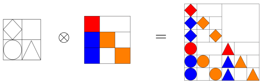
(g)

Figure 1: Visualization of some useful group structures. Figure 1(a) is a block upper-triangular group with $k=2$. Figure 1(b) is a block lower-triangular group with $k=2$. Figure 1(c) is a block Heisenberg group with $k_{1}=2$ and $k_{2}=4$, which is a hierarchical extension of Figure 1(b). Figure 1(d) is a group conjugation of Figure 1(b) by a permutation matrix. Figure 1(e) is a sparse Cholesky group. Figure 1(f) is a triangular-Toeplitz group. Figure 1(g) is a Kronecker product group, which is a Kronecker product of two (block) lower-triangular groups.

where $\mbox{$\mbox{$\mathbf{G}$}$}_{t}=\mathbb{E}_{\scaleto{q_{t}\mathstrut}{6pt}}\left[\nabla_{w}^{2}\ell(\mbox{$\mbox{$\mathbf{w}$}$})\right]-\gamma\mbox{$\mbox{$\mathbf{S}$}$}_{t}$ and $q_{t}(\mbox{$\mbox{$\mathbf{w}$}$}):=\mbox{${\cal N}$}(\mbox{$\mbox{$\mathbf{w}$}$}|\mbox{$\mbox{$\boldsymbol{\mu}$}$}_{t},\mbox{$\mbox{$\mathbf{S}$}$}_{t})$. By setting $0<\beta<1$ and $\gamma=1$, we obtain a second-order update with a moving average on $\mathbf{S}$, where the correction colored in red is added to handle the positive-definite constraint. Lin et al. (2020) study (4) in doubly stochastic settings (e.g., stochastic variational inference using (1)), where noise comes from the mini-batch sampling and the Monte Carlo approximation to the expectations.

The structured natural-gradient method generalizes several NGD methods including gradient-free methods (Glasmachers et al., 2010) and these second-order methods  (Lin et al., 2020; Khan et al., 2018). We could obtain adaptive-gradient methods from a second-order update by using the Gauss-Newton approximation or randomized linear algebra to approximate the Hessian. In this paper, we show that new structured second-order methods for (1) can be obtained by performing NGD for (1) with structured Gaussians. We further show that these structured methods preserve a structural invariance. Finally, we test these structured methods on problems of numerical optimization and deep learning.

2 Tractable NGD for structured Gaussians

The structured natural-gradient method (Lin et al., 2021) is a systematic approach to incorporate flexible structured covariances with simple updates. We will show that structured second-order methods for problem (1) with a structural invariance can be easily derived from these NGD updates.

We use $\mathcal{S}_{++}^{p\times p}$, $\mathcal{S}^{p\times p}$, and $\mathrm{GL}^{p\times p}$ to denote the set of symmetric positive definite matrices, symmetric matrices, and invertible matrices, respectively. We define map $\mbox{$\mbox{$\mathbf{h}$}$}()$ on matrix $\mathbf{M}$ as $\mbox{$\mbox{$\mathbf{h}$}$}(\mbox{$\mbox{$\mathbf{M}$}$}):=\mbox{$\mbox{$\mathbf{I}$}$}+\mbox{$\mbox{$\mathbf{M}$}$}+\mbox{$\frac{1}{2}$}\mbox{$\mbox{$\mathbf{M}$}$}^{2}$.

2.1 Full covariance

We consider a $p$-dimensional Gaussian distribution $q(\mbox{$\mbox{$\mathbf{w}$}$})=\mbox{${\cal N}$}(\mbox{$\mbox{$\mathbf{w}$}$}|\mbox{$\mbox{$\boldsymbol{\mu}$}$},\mbox{$\mbox{$\mathbf{S}$}$}^{-1})$, where $\mbox{$\mbox{$\mathbf{S}$}$}\in\mathcal{S}_{++}^{p\times p}$ is the precision matrix and $\mbox{$\mbox{$\boldsymbol{\Sigma}$}$}=\mbox{$\mbox{$\mathbf{S}$}$}^{-1}$ is the covariance matrix. We consider the following covariance structure $\mbox{$\mbox{$\mathbf{S}$}$}=\mbox{$\mbox{$\mathbf{B}$}$}\mbox{$\mbox{$\mathbf{B}$}$}^{T}$, where $\mbox{$\mbox{$\mathbf{B}$}$}\in\mathrm{GL}^{p\times p}$ is an invertible matrix. Using the structured NGD method, the update for (1) is expressed as:

$$\begin{split}\mbox{$\mbox{$\boldsymbol{\mu}$}$}_{t+1}&\leftarrow\mbox{$\mbox{$\boldsymbol{\mu}$}$}_{t}-\beta\mbox{$\mbox{$\mathbf{S}$}$}_{t}^{-1}\mbox{$\mbox{$\mathbf{g}$}$}_{\mu_{t}}\\ \mbox{$\mbox{$\mathbf{B}$}$}_{t+1}&\leftarrow\mbox{$\mbox{$\mathbf{B}$}$}_{t}\mathbf{h}\big{(}\beta\mbox{$\mbox{$\mathbf{B}$}$}_{t}^{-1}\mbox{$\mbox{$\mathbf{g}$}$}_{\Sigma_{t}}\mbox{$\mbox{$\mathbf{B}$}$}_{t}^{-T}\big{)},\end{split}$$ (5)

where $\mbox{$\mbox{$\mathbf{g}$}$}_{\mu}$ and $\mbox{$\mbox{$\mathbf{g}$}$}_{\Sigma}$ are vanilla gradients for $\boldsymbol{\mu}$ and $\boldsymbol{\Sigma}$. We can show in (5), $\mbox{$\mbox{$\mathbf{B}$}$}_{t+1}\in\mathrm{GL}^{p\times p}$ whenever $\mbox{$\mbox{$\mathbf{B}$}$}_{t}\in\mathrm{GL}^{p\times p}$. Thus, $\mbox{$\mbox{$\mathbf{B}$}$}_{t+1}$ is invertible if initial $\mbox{$\mbox{$\mathbf{B}$}$}_{0}$ is invertible.

By Stein’s identity (Opper & Archambeau, 2009), we have

$$\begin{split}\mbox{$\mbox{$\mathbf{g}$}$}_{\mu}=\mathbb{E}_{\scaleto{q\mathstrut}{6pt}}{\left[\nabla_{w}\ell(\mbox{$\mbox{$\mathbf{w}$}$})\right]},\,\,\,\,\,\mbox{$\mbox{$\mathbf{g}$}$}_{\Sigma}=\mbox{$\frac{1}{2}$}\mathbb{E}_{\scaleto{q\mathstrut}{6pt}}{\left[\nabla_{w}^{2}\ell(\mbox{$\mbox{$\mathbf{w}$}$})\right]}-\frac{\gamma}{2}\mbox{$\mbox{$\mathbf{S}$}$}\end{split}$$ (6)

Using $\mbox{$\mbox{$\mathbf{S}$}$}=\mbox{$\mbox{$\mathbf{B}$}$}\mbox{$\mbox{$\mathbf{B}$}$}^{T}$ and (6), the update in (5) can be expressed as a second-order update as (4) in terms of $\boldsymbol{\mu}$ and $\mathbf{S}$.

$$\mbox{$\mbox{$\boldsymbol{\mu}$}$}_{t+1} \leftarrow\mbox{$\mbox{$\boldsymbol{\mu}$}$}_{t}-\beta\mbox{$\mbox{$\mathbf{S}$}$}_{t}^{-1}\mathbb{E}_{\scaleto{q_{t}\mathstrut}{6pt}}{\left[\nabla_{w}\ell(\mbox{$\mbox{$\mathbf{w}$}$})\right]}$$

$$\mbox{$\mbox{$\mathbf{S}$}$}_{t+1} \leftarrow(1-\beta\gamma)\mbox{$\mbox{$\mathbf{S}$}$}_{t}+\beta\mathbb{E}_{\scaleto{q_{t}\mathstrut}{6pt}}\left[\nabla_{w}^{2}\ell(\mbox{$\mbox{$\mathbf{w}$}$})\right]{+\color[rgb]{1,0,0}\frac{\beta^{2}}{2}\mbox{$\mbox{$\mathbf{G}$}$}_{t}\mbox{$\mbox{$\mathbf{S}$}$}_{t}^{-1}\mbox{$\mbox{$\mathbf{G}$}$}_{t}}+O(\beta^{3})$$

where $O(\beta^{3})$ contains higher order terms.

Using (6) and approximating the expectations in (5) at the mean $\boldsymbol{\mu}$, we obtain an update for (1), where $\mbox{$\mbox{$\mathbf{S}$}$}=\mbox{$\mbox{$\mathbf{B}$}$}\mbox{$\mbox{$\mathbf{B}$}$}^{T}$.

Since (1) only contains $\boldsymbol{\mu}$, we can view $\mathbf{B}$ in (7) as an axillary variable induced by the (hidden) geometry of Gaussian distribution. Compared to the classical geometric interpretation for Newton’s method, this new view allows us to handle the positive-definite constraint and exploit structures in $\mathbf{B}$.

Moreover, update (7) is invariant to any invertible linear transformation like Newton’s method for (1). Consider a linear transformation $\mbox{$\mbox{$\boldsymbol{\mu}$}$}=\mbox{$\mbox{$\mathbf{K}$}$}\mbox{$\mbox{$\mathbf{y}$}$}$ of the variable $\boldsymbol{\mu}$ in the original problem (1), where $\mbox{$\mbox{$\mathbf{K}$}$}\in\mathrm{GL}^{p\times p}$ is an known invertible matrix. Let $f(\mbox{$\mbox{$\mathbf{y}$}$}):=\ell(\mbox{$\mbox{$\mathbf{K}$}$}\mbox{$\mbox{$\mathbf{y}$}$})$ be a new loss function. The update for a new problem $\min_{y\in\text{missing}^{p}}f(\mbox{$\mbox{$\mathbf{y}$}$})$ is

$$\begin{split}\mbox{$\mbox{$\mathbf{y}$}$}_{t+1}&\leftarrow\mbox{$\mbox{$\mathbf{y}$}$}_{t}-\beta\mbox{$\mbox{$\mathbf{C}$}$}_{t}^{-T}\mbox{$\mbox{$\mathbf{C}$}$}_{t}^{-1}\nabla_{y}f(\mbox{$\mbox{$\mathbf{y}$}$}_{t})\\ \mbox{$\mbox{$\mathbf{C}$}$}_{t+1}&\leftarrow\mbox{$\mbox{$\mathbf{C}$}$}_{t}\mathbf{h}\big{(}\frac{\beta}{2}(\mbox{$\mbox{$\mathbf{C}$}$}_{t}^{-1}\nabla_{y}^{2}f(\mbox{$\mbox{$\mathbf{y}$}$}_{t})\mbox{$\mbox{$\mathbf{C}$}$}_{t}^{-T}-\gamma\mbox{$\mbox{$\mathbf{I}$}$})\big{)}.\end{split}$$

By the construction, we have $\mbox{$\mbox{$\boldsymbol{\mu}$}$}_{0}\mspace{-4.0mu}=\mspace{-4.0mu}\mbox{$\mbox{$\mathbf{K}$}$}\mbox{$\mbox{$\mathbf{y}$}$}_{0}$. Since $\mathbf{K}$ is known, we can initialize $\mbox{$\mbox{$\mathbf{C}$}$}_{0}$ and $\mbox{$\mbox{$\mathbf{B}$}$}_{0}$ so that $\mbox{$\mbox{$\mathbf{C}$}$}_{0}\mspace{-4.0mu}=\mspace{-4.0mu}\mbox{$\mbox{$\mathbf{K}$}$}^{T}\mbox{$\mbox{$\mathbf{B}$}$}_{0}\mspace{-3.0mu}\in\mspace{-3.0mu}\mathrm{GL}^{p\times p}$.

By induction, the following relationships hold. $\mbox{$\mbox{$\mathbf{C}$}$}_{t+1}=\mbox{$\mbox{$\mathbf{K}$}$}^{T}\mbox{$\mbox{$\mathbf{B}$}$}_{t+1}$ and $\mbox{$\mbox{$\boldsymbol{\mu}$}$}_{t+1}=\mbox{$\mbox{$\mathbf{K}$}$}\mbox{$\mbox{$\mathbf{y}$}$}_{t+1}$ for any $t\geq 0$.

Since $\mbox{$\mbox{$\boldsymbol{\mu}$}$}_{t+1}=\mbox{$\mbox{$\mathbf{K}$}$}\mbox{$\mbox{$\mathbf{y}$}$}_{t+1}$, we have $f(\mbox{$\mbox{$\mathbf{y}$}$}_{t+1})=\ell(\mbox{$\mbox{$\mathbf{K}$}$}\mbox{$\mbox{$\mathbf{y}$}$}_{t+1})=\ell(\mbox{$\mbox{$\boldsymbol{\mu}$}$}_{t+1})$. This expression shows that the update on $f$ is also the same as that on $\ell$ at each iteration. Thus, this update is invariant to any invertible linear transformation $\mbox{$\mbox{$\mathbf{K}$}$}\mspace{-3.0mu}\in\mspace{-3.0mu}\mathrm{GL}^{p\times p}$.

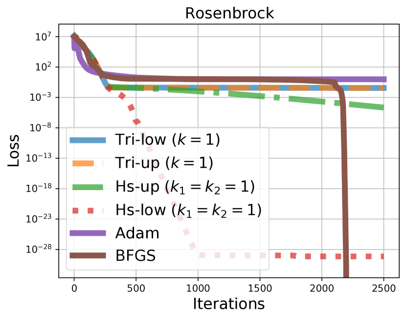
(a)

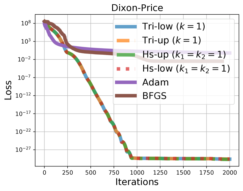
(b)

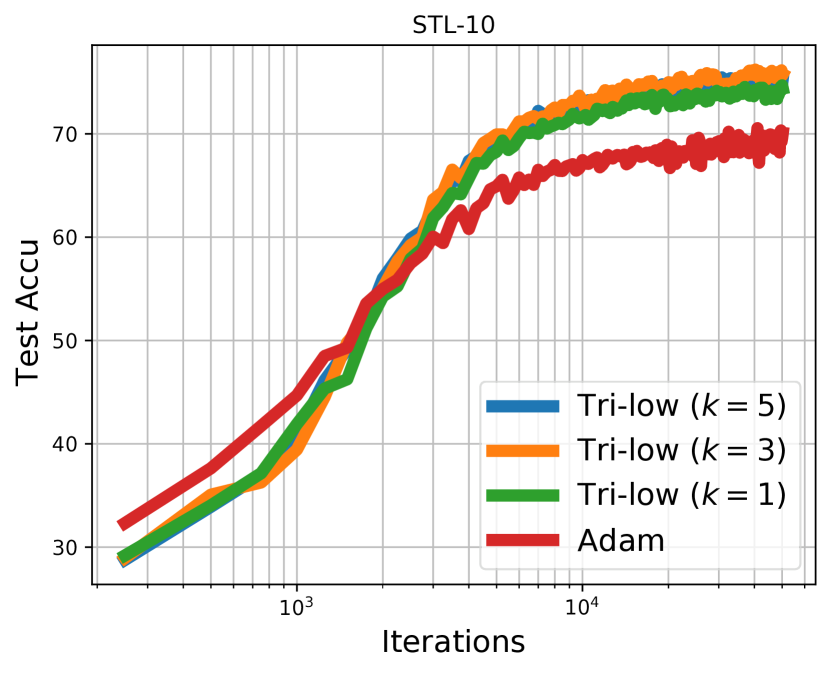
(c)

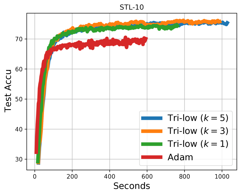
(d)

Figure 2: The performances of our updates for deterministic optimization and deep learning optimization. Fig. 2(a)-2(b) show the performances using structured Newton’s updates to optimize non-separable, valley-shaped, 200-dimensional functions, where our structured second-order updates only require to compute diagonal entries of Hessian and Hessian-vector products. Our updates with a lower Heisenberg structure in the precision form converge faster than BFGS and Adam. Fig. 2(c)-2(d) shows the performances for optimization of a CNN using a Kronecker product group structure, where our adaptive structured updates ($O(k|\mbox{$\mbox{$\boldsymbol{\mu}$}$}|)$) have a linear iteration cost like Adam ($O(|\mbox{$\mbox{$\boldsymbol{\mu}$}$}|)$) and are automatically parallelized by Auto-Diff. Our updates achieve higher test accuracy ($75.8\%$) than Adam ($69.5\%$).

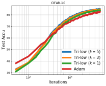
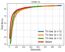
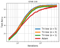
Figure 3: The performances of our updates on the same CNN model on two more datasets. Our updates achieve higher test accuracy ($85.0\%$ on “CIFAR-10”, $55.2\%$ on “CIFAR-100”) than Adam ($82.3\%$ on “CIFAR-10”, $53.3\%$ on “CIFAR-100”).

2.2 Structured covariances

To construct structured covariances, we will use structured restrictions of $\mathrm{GL}^{p\times p}$. Note that $\mathrm{GL}^{p\times p}$ is a general linear group (GL group) (Belk, 2013). Structured restrictions give us subgroups of $\mathrm{GL}^{p\times p}$. We will first discuss a block triangular group. More structures are illustrated in Fig. 1.

${\cal{B}_{\text{up}}}(k)$ denotes the block upper-triangular $p$-by-$p$ matrice space, where $k$ is the block size with $0\leq k\leq p$, $d_{0}=p-k$, and ${\cal D}^{d_{0}\times d_{0}}_{++}$ is a diagonal and invertible matrice space.

$${\cal{B}_{\text{up}}}(k)=\Big{\{}\begin{bmatrix}\mbox{$\mbox{$\mathbf{B}$}$}_{A}&\mbox{$\mbox{$\mathbf{B}$}$}_{B}\\ \mathbf{0}&\mbox{$\mbox{$\mathbf{B}$}$}_{D}\end{bmatrix}\Big{|} \mbox{$\mbox{$\mathbf{B}$}$}_{A}\in\mathrm{GL}^{k\times k},\,\,\mbox{$\mbox{$\mathbf{B}$}$}_{D}\in{\cal D}^{d_{0}\times d_{0}}_{++}\Big{\}}$$

${\cal{B}_{\text{up}}}(k)$ is indeed a matrix (Lie) group closed under matrix multiplication. Its members are all invertible matrices.

By the structured NGD method, we define another set for ${\cal{B}_{\text{up}}}(k)$, where ${\cal D}^{d_{0}\times d_{0}}$ is the diagonal matrix space.

$${\cal{M}_{\text{up}}}(k)=\Big{\{}\begin{bmatrix}\mbox{$\mbox{$\mathbf{M}$}$}_{A}&\mbox{$\mbox{$\mathbf{M}$}$}_{B}\\ \mathbf{0}&\mbox{$\mbox{$\mathbf{M}$}$}_{D}\end{bmatrix}\Big{|} \mbox{$\mbox{$\mathbf{M}$}$}_{A}\in{\cal S}^{k\times k},\,\,\mbox{$\mbox{$\mathbf{M}$}$}_{D}\in{\cal D}^{d_{0}\times d_{0}}\Big{\}}$$

Set ${\cal{M}_{\text{up}}}(k)$, which is indeed a Lie sub-algebra, is designed for ${\cal{B}_{\text{up}}}(k)$ so that $\mbox{$\mbox{$\mathbf{h}$}$}(\mbox{$\mbox{$\mathbf{M}$}$})\in{\cal{B}_{\text{up}}}(k)$ whenever $\mbox{$\mbox{$\mathbf{M}$}$}\in{\cal{M}_{\text{up}}}(k)$.

Now, consider a $p$-dimensional Gaussian distribution $q(\mbox{$\mbox{$\mathbf{w}$}$})=\mbox{${\cal N}$}(\mbox{$\mbox{$\mathbf{w}$}$}|\mbox{$\mbox{$\boldsymbol{\mu}$}$},\mbox{$\mbox{$\mathbf{S}$}$}^{-1})$, where $\mbox{$\mbox{$\mathbf{S}$}$}\in\mathcal{S}_{++}^{p\times p}$ is the precision. We consider the following covariance structure $\mbox{$\mbox{$\mathbf{S}$}$}=\mbox{$\mbox{$\mathbf{B}$}$}\mbox{$\mbox{$\mathbf{B}$}$}^{T}$, where $\mbox{$\mbox{$\mathbf{B}$}$}\in{\cal{B}_{\text{up}}}(k)$ is a member of the group. Using the structured NGD method, the update for (1) is expressed as:

$$\begin{split}\mbox{$\mbox{$\boldsymbol{\mu}$}$}_{t+1}&\leftarrow\mbox{$\mbox{$\boldsymbol{\mu}$}$}_{t}-\beta\mbox{$\mbox{$\mathbf{S}$}$}_{t}^{-1}\mbox{$\mbox{$\mathbf{g}$}$}_{\mu_{t}}\\ \mbox{$\mbox{$\mathbf{B}$}$}_{t+1}&\leftarrow\mbox{$\mbox{$\mathbf{B}$}$}_{t}\mbox{$\mbox{$\mathbf{h}$}$}\left(\beta\mbox{$\mbox{$\mathbf{C}$}$}_{\text{up}}\odot\kappa_{\text{up}}\big{(}2\mbox{$\mbox{$\mathbf{B}$}$}_{t}^{-1}\mbox{$\mbox{$\mathbf{g}$}$}_{\Sigma_{t}}\mbox{$\mbox{$\mathbf{B}$}$}_{t}^{-T}\big{)}\right)\end{split}$$ (8)

where $\odot$ is the element-wise product, $\kappa_{\text{up}}(\mbox{$\mbox{$\mathbf{X}$}$})$ extracts non-zero entries of ${\cal{M}_{\text{up}}}(k)$ from $\mathbf{X}$ so that $\kappa_{\text{up}}(\mbox{$\mbox{$\mathbf{X}$}$})\in{\cal{M}_{\text{up}}}(k)$ and $\mbox{$\mbox{$\mathbf{C}$}$}_{\text{up}}$ is a constant matrix defined below.

$$\mbox{$\mbox{$\mathbf{C}$}$}_{\text{up}}=\begin{bmatrix}\mbox{$\frac{1}{2}$}\mbox{$\mbox{$\mathbf{J}$}$}_{A}&\mbox{$\mbox{$\mathbf{J}$}$}_{B}\\ \mathbf{0}&\mbox{$\frac{1}{2}$}\mbox{$\mbox{$\mathbf{I}$}$}_{D}\end{bmatrix}\in{\cal{M}_{\text{up}}}(k)$$

where $\mathbf{J}$ is a matrix of ones and factor $\frac{1}{2}$ appears in the symmetric part of ${\mbox{$\mbox{$\mathbf{C}$}$}}_{\text{up}}$.

Update (8) preserves the group structure: $\mbox{$\mbox{$\mathbf{B}$}$}_{t+1}\in{\cal{B}_{\text{up}}}(k)$ if $\mbox{$\mbox{$\mathbf{B}$}$}_{k}\in{\cal{B}_{\text{up}}}(k)$. When $k=p$, ${\cal{B}_{\text{up}}}(k)$ becomes the invertible matrix space $\mathrm{GL}^{p\times p}$. Therefore, the update in (8) recovers the update in (5) with a complete covariance structure when $k=p$. Similarly, the update in (8) becomes a NGD update with a diagonal covariance when $k=0$. When $0<k<p$, (8) becomes a NGD update with a structured covariance.

We obtain an update for problem (1) by approximating the expectations in (8) at $\boldsymbol{\mu}$ and using (6), where $\mbox{$\mbox{$\mathbf{S}$}$}=\mbox{$\mbox{$\mathbf{B}$}$}\mbox{$\mbox{$\mathbf{B}$}$}^{T}$.

We can similarly show that this update (9) is invariant to any transformation $\mbox{$\mbox{$\mathbf{K}$}$}^{T}\in{\cal{B}_{\text{up}}}(k)$. Therefore, the update enjoys a group structural invariance since ${\cal{B}_{\text{up}}}(k)$ is a group.

Thanks to the sparsity of group ${\cal{B}_{\text{up}}}(k)$ (Lin et al., 2021), the update in (9) has low time complexity $O(k^{2}p)$. We compute $\mbox{$\mbox{$\mathbf{S}$}$}^{-1}\nabla_{\mu}\ell(\mbox{$\mbox{$\boldsymbol{\mu}$}$})$ and $\mbox{$\mbox{$\mathbf{B}$}$}\mbox{$\mbox{$\mathbf{h}$}$}(\mbox{$\mbox{$\mathbf{M}$}$})$ in $O(k^{2}p)$ since $\mathbf{B}$ and $\mbox{$\mbox{$\mathbf{h}$}$}(\mbox{$\mbox{$\mathbf{M}$}$})$ are in ${\cal{B}_{\text{up}}}(k)$. We compute/approximate diagonal entries of Hessian $\nabla_{\mu}^{2}\ell(\mbox{$\mbox{$\boldsymbol{\mu}$}$})$ and use $k$ Hessian-vector-products for non-zero entries of $\kappa_{\text{up}}\big{(}\mbox{$\mbox{$\mathbf{B}$}$}^{-1}\nabla_{\mu}^{2}\ell(\mbox{$\mbox{$\boldsymbol{\mu}$}$})\mbox{$\mbox{$\mathbf{B}$}$}^{-T}\big{)}$ (see Eq. (54) in Appx J.1.7 of Lin et al. (2021)). We store non-zero entries of $\mathbf{B}$ with space complexity $O((k+1)p)$.

Lin et al. (2021) show that there is a block arrowhead structure (O’leary & Stewart, 1990) over $\mbox{$\mbox{$\mathbf{S}$}$}_{\text{up}}=\mbox{$\mbox{$\mathbf{B}$}$}\mbox{$\mbox{$\mathbf{B}$}$}^{T}$:

$$\mbox{$\mbox{$\mathbf{S}$}$}_{\text{up}} =\begin{bmatrix}\mbox{$\mbox{$\mathbf{B}$}$}_{A}\mbox{$\mbox{$\mathbf{B}$}$}_{A}^{T}+\mbox{$\mbox{$\mathbf{B}$}$}_{B}\mbox{$\mbox{$\mathbf{B}$}$}_{B}^{T}&\mbox{$\mbox{$\mathbf{B}$}$}_{B}\mbox{$\mbox{$\mathbf{B}$}$}_{D}\\ \mbox{$\mbox{$\mathbf{B}$}$}_{D}\mbox{$\mbox{$\mathbf{B}$}$}_{B}^{T}&\mbox{$\mbox{$\mathbf{B}$}$}_{D}^{2}\end{bmatrix}$$

and over $\mbox{$\mbox{$\boldsymbol{\Sigma}$}$}_{\text{up}}=\mbox{$\mbox{$\mathbf{S}$}$}_{\text{up}}^{-1}$, which has a low-rank structure:

$$\mbox{$\mbox{$\boldsymbol{\Sigma}$}$}_{\text{up}} =\mbox{$\mbox{$\mathbf{U}$}$}_{k}\mbox{$\mbox{$\mathbf{U}$}$}_{k}^{T}+\begin{bmatrix}\mathbf{0}&\mathbf{0}\\ \mathbf{0}&\mbox{$\mbox{$\mathbf{B}$}$}_{D}^{-2}\end{bmatrix};\,\,\,\,\mbox{$\mbox{$\mathbf{U}$}$}_{k}=\begin{bmatrix}-\mbox{$\mbox{$\mathbf{B}$}$}_{A}^{-T}\\ \mbox{$\mbox{$\mathbf{B}$}$}_{D}^{-1}\mbox{$\mbox{$\mathbf{B}$}$}_{B}^{T}\mbox{$\mbox{$\mathbf{B}$}$}_{A}^{-T}\end{bmatrix}$$

where $\mbox{$\mbox{$\mathbf{U}$}$}_{k}$ is a rank-$k$ matrix since $\mbox{$\mbox{$\mathbf{B}$}$}_{A}^{-T}$ is invertible.

Similarly, we define a lower-triangular group ${\cal{B}_{\text{low}}}(k)$.

$${\cal{B}_{\text{low}}}(k)=\Big{\{}\begin{bmatrix}\mbox{$\mbox{$\mathbf{B}$}$}_{A}&\mathbf{0}\\ \mbox{$\mbox{$\mathbf{B}$}$}_{C}&\mbox{$\mbox{$\mathbf{B}$}$}_{D}\end{bmatrix}\Big{|} \mbox{$\mbox{$\mathbf{B}$}$}_{A}\in\mathrm{GL}^{k\times k},\,\,\mbox{$\mbox{$\mathbf{B}$}$}_{D}\in{\cal D}^{d_{0}\times d_{0}}_{++}\Big{\}}$$

The update obtained from the structured NGD method with a structure $\mbox{$\mbox{$\mathbf{B}$}$}\in{\cal{B}_{\text{low}}}(k)$ has a low-rank structure in precision $\mbox{$\mbox{$\mathbf{S}$}$}_{\text{low}}=\mbox{$\mbox{$\mathbf{B}$}$}\mbox{$\mbox{$\mathbf{B}$}$}^{T}$. Likewise, the update with a structure $\mbox{$\mbox{$\mathbf{B}$}$}\in{\cal{B}_{\text{up}}}(k)$ has a low-rank structure in covariance $\mbox{$\mbox{$\mathbf{S}$}$}_{\text{up}}^{-1}=(\mbox{$\mbox{$\mathbf{B}$}$}\mbox{$\mbox{$\mathbf{B}$}$}^{T})^{-1}$. We can show that they are structured second-order updates for (1) with a structural invariance when we approximate the expectations at the mean.

A more flexible structure is to construct a hierarchical structure inspired by the Heisenberg group (Schulz & Seesanea, 2018) by replacing a diagonal group in $\mbox{$\mbox{$\mathbf{B}$}$}_{D}$ with a block triangular group, where $0\leq k_{1}+k_{2}\leq p$ and $d_{0}=p-k_{1}-k_{2}$

$${\cal B}_{\text{up}}(k_{1},k_{2})=\Big{\{}\begin{bmatrix}\mbox{$\mbox{$\mathbf{B}$}$}_{A}&\mbox{$\mbox{$\mathbf{B}$}$}_{B}\\ \mathbf{0}&\mbox{$\mbox{$\mathbf{B}$}$}_{D}\end{bmatrix}\Big{|}\mbox{$\mbox{$\mathbf{B}$}$}_{D}=\begin{bmatrix}\mbox{$\mbox{$\mathbf{B}$}$}_{D_{1}}&\mbox{$\mbox{$\mathbf{B}$}$}_{D_{2}}\\ \mathbf{0}&\mbox{$\mbox{$\mathbf{B}$}$}_{D_{4}}\end{bmatrix}\Big{\}}$$

where $\mbox{$\mbox{$\mathbf{B}$}$}_{A}\in\mathrm{GL}^{k_{1}\times k_{1}}$, $\mbox{$\mbox{$\mathbf{B}$}$}_{D_{1}}\in{\cal D}_{++}^{d_{0}\times d_{0}}$, $\mbox{$\mbox{$\mathbf{B}$}$}_{D_{4}}\in\mathrm{GL}^{k_{2}\times k_{2}}$.

If the Hessian $\nabla_{\mu}^{2}\ell(\mbox{$\mbox{$\boldsymbol{\mu}$}$})$ has a model-specific structure, we could use a customized group to capture such a structure in the precision. For example, the Hessian of layer-wise matrix weights of a NN admits a Kronecker form. We can use a Kronecker product group to capture such structure. This group can reduce the time complexity from the quadratic complexity to a linear one in $k$ (see Appx. I.1 of Lin et al. (2021) and Fig. 2). By approximating the expectations at the mean and the Hessian by the Gauss-Newton, the structured NGD method gives us a structured adaptive update for NNs. This update also enjoys a group structural invariance. Existing structured adaptive methods such as KFAC (Martens & Grosse, 2015) and Shampoo (Gupta et al., 2018) do not have the invariance. Moreover, our update is different from existing NG methods for NN. These existing NG methods use the empirical Fisher defined by $\ell$ while ours uses the the exact Fisher of the Gaussian $q$. Our method does not have the issue studied by Kunstner et al. (2019).

We could obtain more structured second-order updates by using many subgroups (e.g., invertible circulant matrix groups, invertible triangular-Toeplitz matrix groups) of the $\mathrm{GL}^{p\times p}$ group and groups obtained from existing groups via the group conjugation by an element of the orthogonal group.

3 Numerical Results

3.1 Structured Second-order Optimization

We consider 200-dimensional ($p=200$), non-separable, valley-shaped test functions for optimization: Rosenbrock: $\ell_{\text{rb}}(\mbox{$\mbox{$\mathbf{w}$}$})=\frac{1}{p}\sum_{i=1}^{p-1}\big{[}100(w_{i+1}-w_{i})^{2}+(w_{i}-1)^{2}\big{]}$, and Dixon-Price: $\ell_{\text{dp}}(\mbox{$\mbox{$\mathbf{w}$}$})=\frac{1}{p}\big{[}(w_{i}-1)^{2}+\sum_{i=2}^{p}i(2w_{i}^{2}-w_{i-1})^{2}\big{]}$. We test our structured second-order updates for (1), where we set $\gamma=1$ in our updates. We consider these structures in the precision $\mathbf{S}$: the upper triangular structure (denoted by “Tri-up”), the lower triangular structure (denoted by “Tri-low”), the upper Heisenberg structure (denoted by “Hs-up”), and the lower Heisenberg structure (denoted by “Hs-low”), where second-order information is used. For our updates, we compute Hessian-vector products and diagonal entries of the Hessian without computing the whole Hessian. We consider baseline methods: the BFGS method from SciPy and the Adam optimizer, where the step-size is tuned for Adam. Figure 2(a)-2(b) show the performances of all methods, where our updates with a lower Heisenberg structure converge faster than BFGS and Adam.

3.2 Optimization for Deep Learning

We consider a CNN model with 9 hidden layers. For a smooth objective, we use average pooling and GELU (Hendrycks & Gimpel, 2016) as activation functions. We employ $L_{2}$ regularization with weight $10^{-2}$. We set $\gamma=1$ in our updates. We train the model with our structured adaptive updates (see Appx. I of Lin et al. (2021)) for matrix weights at each layer of NN on datasets “STL-10”, “CIFAR-10”, “CIFAR-100”. We use a Kronecker product group structure of two lower-triangular groups (referred to as “Tri-low”) for computational complexity reduction. We train the model with mini-batches. We compare our updates to Adam, where the step-size for each method is tuned by grid search. We use the same initialization and hyper-parameters in all methods. We report results in terms of test accuracy, where we average the results over 5 runs with distinct random seeds. From Figures 2-3, we can see our structured updates have a linear iteration cost like Adam while achieve higher test accuracy.

4 Conclusion

We propose structured second-order updates for unconstrained optimization and structured adaptive updates for NNs. These updates seem to be promising. An interesting direction is to evaluate these updates in large-scale settings.

References

• Baba (1981) Baba, N. Convergence of a random optimization method for constrained optimization problems. Journal of Optimization Theory and Applications, 33(4):451–461, 1981.
• Belk (2013) Belk, J. Lecture Notes: Matrix Groups. http://faculty.bard.edu/belk/math332/MatrixGroups.pdf, 2013. Accessed: 2021/02.
• Beyer (2001) Beyer, H.-G. The theory of evolution strategies. Springer Science & Business Media, 2001.
• Glasmachers et al. (2010) Glasmachers, T., Schaul, T., Yi, S., Wierstra, D., and Schmidhuber, J. Exponential natural evolution strategies. In Proceedings of the 12th annual conference on Genetic and evolutionary computation, pp.  393–400, 2010.
• Gupta et al. (2018) Gupta, V., Koren, T., and Singer, Y. Shampoo: Preconditioned Stochastic Tensor Optimization. In Proceedings of the 35th International Conference on Machine Learning, pp.  1842–1850, 2018.
• Hazan et al. (2016) Hazan, E., Levy, K. Y., and Shalev-Shwartz, S. On graduated optimization for stochastic non-convex problems. In International conference on machine learning, pp. 1833–1841. PMLR, 2016.
• Hendrycks & Gimpel (2016) Hendrycks, D. and Gimpel, K. Gaussian error linear units (gelus). arXiv preprint arXiv:1606.08415, 2016.
• Khan & Rue (2020) Khan, M. E. and Rue, H. Learning-algorithms from Bayesian principles. 2020. https://emtiyaz.github.io/papers/learning_from_bayes.pdf.
• Khan et al. (2017) Khan, M. E., Lin, W., Tangkaratt, V., Liu, Z., and Nielsen, D. Variational adaptive-Newton method for explorative learning. arXiv preprint arXiv:1711.05560, 2017.
• Khan et al. (2018) Khan, M. E., Nielsen, D., Tangkaratt, V., Lin, W., Gal, Y., and Srivastava, A. Fast and scalable Bayesian deep learning by weight-perturbation in Adam. In Proceedings of the 35th International Conference on Machine Learning, pp.  2611–2620, 2018.
• Kunstner et al. (2019) Kunstner, F., Balles, L., and Hennig, P. Limitations of the empirical fisher approximation for natural gradient descent. arXiv preprint arXiv:1905.12558, 2019.
• Leordeanu & Hebert (2008) Leordeanu, M. and Hebert, M. Smoothing-based optimization. In 2008 IEEE Conference on Computer Vision and Pattern Recognition, pp.  1–8. IEEE, 2008.
• Lin et al. (2020) Lin, W., Schmidt, M., and Khan, M. E. Handling the positive-definite constraint in the bayesian learning rule. In International Conference on Machine Learning, pp. 6116–6126. PMLR, 2020.
• Lin et al. (2021) Lin, W., Nielsen, F., Khan, M. E., and Schmidt, M. Tractable structured natural gradient descent using local parameterizations. arXiv preprint arXiv:2102.07405v6, 2021.
• Martens & Grosse (2015) Martens, J. and Grosse, R. Optimizing neural networks with Kronecker-factored approximate curvature. In International Conference on Machine Learning, pp. 2408–2417, 2015.
• Mnih et al. (2016) Mnih, V., Badia, A. P., Mirza, M., Graves, A., Lillicrap, T., Harley, T., Silver, D., and Kavukcuoglu, K. Asynchronous methods for deep reinforcement learning. In International conference on machine learning, pp. 1928–1937. PMLR, 2016.
• Mobahi & Fisher III (2015) Mobahi, H. and Fisher III, J. A theoretical analysis of optimization by gaussian continuation. In Proceedings of the AAAI Conference on Artificial Intelligence, volume 29, 2015.
• O’leary & Stewart (1990) O’leary, D. and Stewart, G. Computing the eigenvalues and eigenvectors of symmetric arrowhead matrices. Journal of Computational Physics, 90(2):497–505, 1990.
• Opper & Archambeau (2009) Opper, M. and Archambeau, C. The variational Gaussian approximation revisited. Neural computation, 21(3):786–792, 2009.
• Schulz & Seesanea (2018) Schulz, E. and Seesanea, A. Extensions of the Heisenberg group by two-parameter groups of dilations. arXiv preprint arXiv:1804.10305, 2018.
• Spall (2005) Spall, J. C. Introduction to stochastic search and optimization: estimation, simulation, and control, volume 65. John Wiley & Sons, 2005.
• Sutton et al. (1998) Sutton, R. S., Barto, A. G., et al. Introduction to reinforcement learning, volume 135. MIT press Cambridge, 1998.
• Teboulle (1992) Teboulle, M. Entropic proximal mappings with applications to nonlinear programming. Mathematics of Operations Research, 17(3):670–690, 1992.
• Williams & Peng (1991) Williams, R. J. and Peng, J. Function optimization using connectionist reinforcement learning algorithms. Connection Science, 3(3):241–268, 1991.
• Zellner (1986) Zellner, A. Bayesian estimation and prediction using asymmetric loss functions. Journal of the American Statistical Association, 81(394):446–451, 1986.