Turbulent Magnetic Dynamos with Halo Lags, Winds, and Jets

Abstract

This paper presents scale invariant/self-similar galactic magnetic dynamo models based on the classic equations, and compares them qualitatively to recently observed magnetic fields in edge-on spiral galaxies. We classify the axially symmetric dynamo magnetic field by its separate sources, advected flux and sub scale turbulence. We neglect the diffusion term under plausible physical conditions. There is a time dependence determined by globally conserved quantities. We show that magnetic scale heights increase with radius and wind velocity. We suggest that AGN outflow is an important element of the large scale galactic dynamo, based on the dynamo action of increasing sub scale vorticity. This leads us to predict a correlation between the morphology of coherent galactic magnetic field (i.e. extended polarized flux) and the presence of an AGN.

1 Introduction and Background

Dynamo theory as an explanation for the magnetic fields in galaxies, including the Milky Way, has a long history both observationally and theoretically. Observational reviews and discussion of the relevant theory may be found in Beck (2015) and Krause (2015). The textbook Klein & Fletcher (2015) discusses the theory and observation with abundant references. Blackman (2015) discusses modern theoretical developments in the theory, although these are not employed in our work.

More recently, a scale invariant version of the classical theory (e.g. Steenbeck, Krause & Rädler, 1966; Moffat, 1978; Henriksen, 2017; Henriksen, Woodfinden and Irwin, 2018a, b; Woodfinden et al., 2019) has had some success. This approach succeeds in isolating and predicting the more common qualitative elements of a galactic magnetic field, much of which is compatible with previous work. Observational data have been enhanced by the CHANG-ES survey, which has been reviewed recently in Irwin et al. (2019). The presence of magnetic spiral ‘arms’ or ‘ropes’ in the radio halos of galaxies was predicted originally by this approach in Henriksen (2017) and subsequent work by this author and colleagues. A key prediction has been supported recently by the inferred magnetic field in the radio halo of the ‘Whale’ galaxy NGC 4631, as described in Mora-Partiarroyo et al. (2019) and Woodfinden et al. (2019).

In parallel to the observational/analytic studies, numerical work has blossomed. This approach studies either the cosmological origin of galactic magnetic fields, or the development from a ‘seed field’ of a galactic dynamo. We do not pretend to review this literature fairly, but we can refer to some that have been brought to our attention.

In the cosmological category we find early work by Wang & Abel (2009) and Beck, Dolag, Lesch et al. (2012), and this has been continued into the present by Pakmor, Marinacci & Springel (2014), Rieder & Teyssier (2016), Rieder & Teyssier (2017a), Rieder & Teyssier (2017b), and Pakmor, Guillet, Pfrommer et al. (2018), among others. The paper, Rieder & Teyssier (2016), is noteworthy for establishing that global, supernovae driven, turbulence during galaxy formation can amplify seed fields to necessary low red shift values. This is really a globally distributed $\alpha/\Omega$ dynamo, in which one finds limiting exponential field growth with time scale $1/\Omega$. Our limiting time dependence found below under the assumption of scale invariance agrees with this behaviour. In Katz, Martin-Alvarez, Devrient (2019) and Martin-Alvarez, Slyz, Devrient (2020) the authors introduce the notion of tracking the cosmological history of a given low Z magnetic field.

The cosmological environment, beyond clusters, is not suitable for the assumption of asymptotic scale invariance because of large scale continuing evolution. The extended infall onto a forming galaxy is a possible exception. However, the numerical work that focuses on the origin and structure of galactic fields should, when smoothed appropriately, correspond to our assumption of self-similarity (including similarity between galaxies). Recent papers in this category by Butsky, Zrake, Kim et al. (2017) and Pakmor, van de Voort, Bieri et al. (2020) are particularly relevant. We will compare our results with theirs in a later discussion after we have presented our calculations and observations.

There is a growing consensus that galactic winds are an essential component of the long lived galactic dynamo. In fact throughout this series of papers on scale invariance, we have found it necessary to include such winds. This was already the case in our original suggestion Henriksen & Irwin (2016), which required halo lag and disc wind to develop an X magnetic field. In the current paper we also call attention to AGN outflows as being possibly a part of the dynamo (see also Predehl, Sunyaev, Becker et al., 2020). The numerical work attempts to reveal the detailed origins of such winds, whereas this paper does not make statements about the wind origin. Rather, we take the wind to be a necessary part of the self-similar, scale-invariant development which we present below.

Recently, several relevant numerical/analytic works have been submitted in draft form to ariv.org. Two papers, Quataert, Jiang & Thompson (2021), Quataert, Thompson & Jiang (2021), have examined galactic winds driven by cosmic rays, either by random diffusion or by streaming along the magnetic field. It appears that diffusion is more effective, but it is not clear that such winds can produce the observed X field at all heights above the disc. An alternate approach in a recent draft, Steinwandel, Dolag, Lesch & Burkert (2021), suggests magnetic pressure can drive a disc outflow, after the field has been amplified by the $\alpha/\Omega$ dynamo. The amplification in the disc is much like that proposed in Butsky, Zrake, Kim et al. (2017). This paper includes the outflow as an integral part of the dynamo. Moreover the paper presents a biconical outflow from the galaxy that might coincide with the large scale soft X-ray emission found in Predehl, Sunyaev, Becker et al. (2020).

The more traditional wind from the disc is driven by vigorous star formation with the consequent super nova explosions. This has not seemed to be efficient enough, but there is a recent, very relevant paper Su, Hopkins, Hayward, Ma et al. (2018). This paper shows in numerical detail how discrete localized supernovae enhance the outflow over what is achieved by smoothly averaging the super nova energy input over the star forming disc.

Recent numerical papers Garaldi, Pakmor & Springel (2021), and Attia, Teyssier, Katz, Kimm et al. (2021) have addressed the problem of primordial magneto genesis. These study the development of primordial magnetic fields at ionization fronts during the recombination due to the well known Biermann battery and a recent mechanism called the Durrive battery. They follow the field and galaxy evolution to the current epoch and find (Garaldi, Pakmor & Springel, 2021) that the different initial field seedings have small ultimate effect. This may be due to the turbulent dynamo occurring naturally and becoming dominant, as found in Rieder & Teyssier (2016).

The application of scale invariance/self-similarity to such complicated physical problems, relies on the whole system of interest attaining an internal asymptotic behaviour. The philosophy is similar to applying thermodynamic laws to the beginning and end of a string of chemical reactions without the intervening details. The numerical work furnishes the physical details at a cost of complexity, while the scale invariance/self-similarity yields only ultimate behaviour, although it is frequently exact.

Our theoretical technique is the same as always in this series, but we have neglected intermediate scale diffusion in favour of other parts of the dynamo, namely small scale (‘fast’) turbulence and outflow/inflow. This allows simpler analytic results for the most part. Halo lag and ‘fast turbulence’ throughout the disc and halo are new parts of the assumed self-similarity, as is the possible contribution of an AGN to the dynamo.

A slightly different approach to understanding the magnetic field in edge-on galaxies has been pioneered, for example, in Ferrière & Terral (2014) and Terral & Ferriere (2017). In this approach, different topological classes of magnetic field are assigned to a galaxy, and then the consequent pattern of Faraday Rotation is carefully calculated. This allows comparison with observations, particularly for the Milky way. These fields are somewhat arbitrary, but in fact they correspond quite closely to our scale invariant dynamo fields.

1.1 Qualitative Model and Philosophy

It helps when interpreting the magnetic field topology that we find, to recall that scale invariant fields must appear self-similar at all resolutions and so they normally only close at infinity. This is true even though the divergence of the field is everywhere zero, so that a field line is never broken. Exceptional cases do arise wherein the field lines close through a singularity, but we do not study these here.

In this paper we study the structure of scale invariant (or self-similar) magnetic dynamo fields, which contain, for the first time, both a rotating halo that lags behind the disc rotation and an accelerating outflow/inflow. Observational examples of halos that are best fit with accelerating outflows are NGC 3556 (Miskolczi et al., 2019) NGC 891 (Schmidt et al., 2019), and NGC 5775 (Heald et al., 2021). We also allow the (scaled) sub scale (also called ‘fast’ elsewhere) turbulent vorticity (sometimes described as hydrodynamic helicity) to increase with latitude in an attempt to imitate an AGN. The usual scale invariant variation of this quantity is proportional to cylindrical radius, and hence it decreases near the axis.

The ‘small’ (i.e. sub resolution scale) scale turbulence must have net hydrodynamic vorticity for the $\alpha$ effect to be present, so we often write sub scale vorticity as synonymous with the $\alpha$ effect. Because of a notational clash with our temporal scale factor $\alpha$, we refer to the effect as the $\alpha_{h}$ effect.

The inclusion of a rotating galactic halo that lags the disc is an important observed feature that we include in the dynamo action. Rotational velocity in the galactic halo gas significantly declines with height above the disc of spiral galaxies (e.g. Rand, 2000; Heald et al., 2007). This ‘halo lag’ inspired a model (Henriksen & Irwin, 2016, = H-I) wherein the halo magnetic field is generated through coupling to the distant halo and/or the intergalactic medium. This model accounts for both the lagging halo rotation and a global magnetic field. The model is dynamical in the sense that pressure and gravity also contribute to the steady state, but it did not include the sub scale turbulent dynamo.

The present formalism follows that in Henriksen, Woodfinden and Irwin (2018a) so the formalism is only briefly introduced in the next section. The scaled lag and wind/accretion are allowed to be variable with the latitude in the halo. However we do not solve for the dynamics of the halo gas. Rather, according to our basic assumption, the halo lag, outflow/inflow, and sub scale helicity are determined in functional form by the scaling symmetry. The time dependence is determined by the global invariants under the scaling symmetry, much as the scale invariant dissipation rate determines the Kolmogorov scaling law in hydrodynamic turbulence.

The H-I model led to a rather coherent field structure. The celebrated ‘X-type’ projected magnetic field (Krause, 2015; Beck, 2015) was present, as were also spiralling field lines (axially symmetric) rising and expanding into the galactic halo. In this paper we wish to determine whether there are characteristic observable galactic magnetic topologies that may distinguish between a dominant $\alpha_{h}$ effect or a dominant macroscopic dynamo. We compare some of our results to the recent catalogue of magnetic fields in the CHANG-ES survey given in Krause, Irwin, Schmidt et al. (2020). All of these images are freely available for download in FITS format at queensu.ca/changes.

2 Basic Theory

We refer to Henriksen, Woodfinden and Irwin (2018a) and references therein for a detailed presentation of scale invariant or self similar classical dynamo theory, including time dependence and axial symmetry. However in this study we set the diffusivity equal to zero, but include a lag in the rotational halo velocity as well as accelerating/decelerating outflow or accretion, from or onto the disc. An innovation is that the sub-scale turbulent helicity is allowed to vary with height in addition to the usual variation with radius. This produces an axial magnetic field that may in reality be generated by jets or nuclear winds.

It is worth discussing briefly the conditions under which we may justifiably neglect the diffusion term in the dynamo equation (Eq. 3) below. If we compare in order of magnitude the terms in the diffusion coefficient $\eta$ and in the sub scale helicity $\alpha_{h}$ to the convection term we obtain respectively the ratios

$$\frac{\eta}{LV},~{}~{}~{}~{}~{}\frac{\alpha_{h}}{V},$$ (1)

where $L$ is a macroscopic spatial scale and $V$ is a macroscopic velocity. One estimate for the diffusion coefficient, $\eta$, is the turbulent value, $u\ell$, where $\ell$ is the sub scale and $u$ is the corresponding sub scale turbulent velocity. We will take this to be $u\approx\alpha_{h}$. Then the first ratio is small in proportion to $(\alpha_{h}/V)(\ell/L)$. It is small compared to the second $\alpha_{h}$ term insofar as $\ell/L$ is small. In the CHANG-ES data, a linear resolution scale on a galaxy is typically several hundred parsecs, which may be regarded as a minimum $L$. The sub scale is on the scale of star formation so that $\ell/L$ is $O(10^{-2})-O(10^{-1})$. Similarly $u/V$ will be small, if $u$ is a turbulent velocity and $V$ is macroscopic.

Another estimate of $\eta$ is as a Bohm type value due to gyrating relativistic electrons in a magnetic field. This suggests

$$\eta\approx\frac{cE_{e}}{3eB},$$ (2)

where $E_{e}$ is the electron total energy and $e$ is the electronic charge in esu. This gives $\eta\approx 1.7\times 10^{13}\gamma_{e}/B$ cgs, where $\gamma_{e}$ is the electron Lorentz factor. For $B\approx 10^{-6}$ Gauss and $\gamma_{e}\approx 10^{5}$ we obtain $1.7\times 10^{24}$ cgs. This is to be compared to $LV$ which is $10^{27}$ cgs for $L\approx 10^{20}$ cm and $V\approx 10^{7}$ cm/s. We conclude that the diffusion is a higher order effect in the general dynamo in the presence of convection.

Moreover, in previous work Henriksen (2017), Henriksen, Woodfinden and Irwin (2018a), we have included the intermediate scale diffusion in our self-similar solutions. These solutions are generally more complicated to obtain, but they do not show qualitative differences with the solutions in this paper. We believe that this is because the mean outflow or inflow dominates the intermediate scale diffusion.

It is difficult to reconcile the kinematic scale invariant symmetry that we assume with the actual observed halo lag (although see H-I). Strictly, a full treatment would require multi dimensional self similarity and so plunge the problem back into partial differential equations (although without the time dimension Carter & Henriksen (1991)). We achieve a reasonable form in this kinematical study with one self-similar variable, by assuming that the dynamo equation holds in a pattern reference frame rotating with the velocity ${\bf v}_{p}=v_{p}(r)\hat{\bf e}_{\phi}$. Here $e_{\phi}$ is the azimuthal unit vector around the rotation axis of the galaxy.

A valid classical dynamo equation in the pattern frame requires Faraday’s law to hold plus the usual dynamo expression for the electric field (e.g. Henriksen, 2017). One finds, starting with Faraday’s law in the systemic frame (assumed inertial), that to first order in $v/c$ Faraday’s equation does hold in the pattern frame provided that the pattern speed is solid body rotation. A solid body rotation does not itself contribute to dynamo action. This permits the magnetic field to be invariant on transforming to this frame of reference. Unfortunately such a uniform rotation does not correspond to the principal rotation of the galaxy. Rather it corresponds to a spiral arm pattern rotation or perhaps the pattern rotation of magnetic spiral arms. Nevertheless the invariance between the pattern frame and the inertial systemic frame means that the observed field should correspond to that found in the pattern frame.

Our total rotational speed will be $v_{p}+v_{s}(z)$, where $v_{s}(z)$ is the halo rotational velocity in the pattern frame, normally a lag relative to $v_{p}$. It would be ideal to have $v_{p}$ constant, if we identify the pattern speed with the galactic thin disc rotation. Unfortunately this choice adds a spurious first order term to the pattern frame Faraday’s equation, namely $-v_{p}B_{r}/(rc)$ added to the time derivative. This term represents the dynamo action of a constant rotation velocity. It may only be neglected compared to the time derivative if our vertical lag rate (that is $\delta$ below) is larger that $v_{p}/r$.

We proceed to solve the classical dynamo equation (Steenbeck, Krause & Rädler, 1966; Moffat, 1978) in the pattern frame for the magnetic vector potential (we set $\eta=0$ which is included in the following equation for reference only)

$$\partial_{t}{\bf A}=\alpha_{h}\nabla\times{\bf A}+{\bf v}\times\nabla\times{\bf A}-\eta\nabla\times\nabla\times{\bf A},$$ (3)

where a scaled magnetic field and the scaled vector potential are related by

$${\bf b}=\nabla\times{\bf A},$$ (4)

$\alpha_{h}$ is the sub-scale turbulent ‘helicity’, and ${\bf v}$ is the global vector velocity of the halo gas.

For Dimensional simplicity, the scaled magnetic field is taken as

$${\bf b}\equiv\frac{{\bf B}}{\sqrt{4\pi\rho}},$$ (5)

where $\rho$ is some arbitrary constant with the Dimension of density. This gives ${\bf b}$ the Dimension of velocity and so ${\bf A}$ has the Dimension of specific angular momentum. The formula for the vector potential requires neglecting an electrostatic field that would result from large scale charge separation after integration of the Faraday’s law. It seems unlikely that a large scale electrostatic field should be important. Such an integration has the additional benefit of allowing the sub scale helicity $\alpha_{h}$ (and the diffusion coefficient $\eta$ where applicable) to vary with position without adding extra terms.

The search for axially symmetric (we use components in cylindrical coordinates), scale invariant solutions of Eqn. 3 requires assuming that

$${\bf A}=\bar{\bf A}(R,Z)e^{(2\delta-\alpha)T},$$ (6)

where the scale invariants (equivalent to the self-similar variables ) in space and time are

$$R\equiv re^{-\delta T},~{}~{}~{}~{}~{}Z\equiv ze^{-\delta T},~{}~{}~{}~{}~{}e^{\alpha T}\equiv(1+\alpha t).$$ (7)

As in Henriksen, Woodfinden and Irwin (2018a) the reciprocal scales in space and times are $\delta$ and $\alpha$, respectively. If there were a fixed spatial scale in the problem then $\delta=0$, while a fixed time scale requires $\alpha=0$. In the latter case our time, $T$, would be defined with $\delta$ replacing $\alpha$. The limit $\alpha=0$ is not strictly equivalent to an exact steady state (e.g. Henriksen, 2017; Henriksen, Woodfinden and Irwin, 2018a, and below). Extensive discussion of the use of such scales may be found in Henriksen (2015), but in a given problem they may be assigned to give numerical quantities.

The other quantities must have the following forms relative to the pattern frame

$${\bf v} = \tilde{\alpha}_{d}\delta Re^{(\delta-\alpha)T}(0,v,w),$$ (8)

$$\alpha_{h} = \tilde{\alpha}_{h}\delta Re^{(\delta-\alpha)T},$$ (9)

$${\bf b} = \bar{b}(R,Z)e^{(\delta-\alpha)T},$$ (10)

where we have allowed only an azimuthal velocity and an outflow/inflow wind component in this study. At this stage the auxiliary functions $\tilde{\alpha}_{h}$ and $v$, $w$ may be arbitrary functions of $R$ and $Z$.

The similarity class ($a$, see e.g. Carter & Henriksen, 1991; Henriksen, 2015) is sometimes used in what follows, and it is given in terms of the ratio of characteristic temporal and spatial scales according to

$$a\equiv\frac{\alpha}{\delta}.$$ (11)

To this point we have described a multi-variable formulation of scale invariance (the invariant scaling follows by holding the self-similar variables constant), wherein the time dependence has been reduced to either a multiplication by a power law or by an exponential, depending on the class $a$. Proceeding with this analysis requires the solution of a partial differential equation in $R$ and $Z$, once the auxiliary functions are given in the same variables. However, inspired mainly by the X-type field structure (e.g. Krause, Irwin, Schmidt et al., 2020), we reduce the problem further in this series of papers by looking for a solution that depends only on the tangent of the halo latitude, in the form

$$\zeta\equiv\frac{Z}{R}\equiv\frac{z}{r}.$$ (12)

Such a solution is found to exist provided that $\tilde{\alpha}_{h}$ and $v$ and $w$ are at most functions of $\zeta$ and now

$$\bar{\bf A}(R,Z)=\tilde{\bf A}(\zeta),~{}~{}~{}~{}~{}\bar{\bf b}(R,Z)=\frac{\tilde{\bf b}(\zeta)}{R}.$$ (13)

For our halo lag description we take the Dimensionless velocity in the pattern frame (referred to as $v_{s}$ earlier)

$$v(\zeta)=-v_{1}|\zeta|$$ (14)

for constant $v_{1}$. With this choice the explicit rotational velocity lag and wind/accretion velocity in this frame, by Eqs. 8 and 7, become respectively

$$v_{\phi}=-\tilde{\alpha}_{h}\delta(v_{1}|z|)e^{-\alpha T},~{}~{}~{}~{}v_{z}=\tilde{\alpha}_{h}w(\zeta)\delta re^{-\delta T}.$$ (15)

When $\tilde{\alpha}_{h}$ is constant, the halo lag, $v_{\phi}$, is linear in $z$, but should $\tilde{\alpha}_{h}$ be linear in $\zeta$ then the the lag is proportional to $z^{2}/r$ (see also Sect. 3.6). The consequent systemic form after adding a constant pattern velocity, $v_{p}$ , is similar to that found dynamically in Henriksen & Irwin (2016). The expression derived there was found to be a reasonable fit to a well measured halo lag galaxy NGC 891 (Oosterloo et al., 2007). We discuss the form of the outflow/inflow factor $w(\zeta)$ in Sect. 3.4, below.

2.1 Time dependence

In this section, we use the logarithmic time, $T$, as defined in Eq. 7 . When we recall that $R=re^{-\delta T}$, we see from Eqns. 10, 13 and 7, that

$${\bf b}\propto e^{(2-a)\delta T}\propto(1+\alpha t)^{(2/a-1)}.$$ (16)

It is now clear that $1/\alpha$ (or $1/\tilde{\alpha}_{h}\alpha$ when $\tilde{\alpha}_{h}$ multiplies $\alpha$ in the definition of $T$ in Eq. 18) may be identified with a characteristic time (growth or decay) for the self-similar dynamo, but that $a$ determines the form of the growth function.

This is where global conserved quantities enter the scale invariant picture. If for example $a=1$, corresponding to a constant global velocity or initial constant ‘seed’ magnetic field, the field increases linearly in time at a rate given by $\alpha$ or $\tilde{\alpha}_{h}\alpha$. If we suppose instead that the the usual magnetic helicity integrated over a volume $V$ is conserved, that is

$$\int~{}{\bf A}\cdot{\bf b}~{}dV=constant,$$ (17)

then the global constant has Dimensions $L^{6}/T^{2}$. This requires $6\delta-2\alpha=0$ for invariance in time, and hence $a=\alpha/\delta=3$. We conclude from Eqn. 16 that the magnetic field must decline as $(1+\alpha t)^{-1/3}$. Such a decline agrees with previous suggestions (e.g. Shukurov et al., 2006; Blackman, 2015).

Conserving the local magnetic helicity density (Moffat, 1978) itself, suggests $L^{3}/T^{2}$ as the physical dimensions of a conserved quantity everywhere (gauge invariant over a closed volume however small), hence $a=3/2$ (a Keplerian value) from $3\delta-2\alpha=0$ and so the field grows slowly as $1+\alpha t)^{1/3}$.

If the macroscopic ‘current’ helicity ${\bf b}\cdot\nabla\times{\bf b}$ is conserved locally, then the local constant has Dimensions $L/T^{2}$ so that $a=1/2$, which gives rapid growth $\propto(1+\alpha t)^{3}$. The volume integrated version of this helicity implies $L^{4}/T^{2}$ whence $a=2$ which implies a steady state. In our numerical studies we normally use $a=1$, which corresponds to either an invariant global velocity or a constant initial ‘seed’ magnetic field. Such a velocity may be set by a flat rotation curve, or possibly by a typical constant outflow velocity. An initial seed field must be determined by cosmology and a theory of galaxy formation (e.g. Wang & Abel, 2009; Beck, Dolag, Lesch et al., 2012; Pakmor, Marinacci & Springel, 2014).

A limiting exponential growth in the dynamo field is given by supposing that there is a global constant with a fixed dimension of reciprocal time. This might be a fixed angular velocity $\Omega$ or possibly a constant rotational lag rate, but in any case the assumption requires $\alpha\rightarrow 0$ so that the relevant quantity is conserved in time. In that case the limit of Eqn. 16 as $\alpha\rightarrow 0$ gives exponential growth as $b\propto e^{2\delta t}$. Here $\delta$ is a reciprocal time characteristic of the magnetized galaxy. If this is $r/v_{\phi}$ then the e-folding time is essentially a rotation period, as might be expected.

3 Separate physical parts of the galactic magnetic dynamo

In this section, we study the magnetic field produced when either the sub scale turbulent dynamo ($\alpha_{h}$ term) or the convective flux freezing in Eqns. 3 is dominant. There are various examples in each case depending on the parameters. We also consider some important combinations of these effects. The objective is to isolate magnetic topology that may reveal which mechanism is important in a magnetized edge on galaxy, Such data have been reported in the recent CHANG-ES catalogue (Krause, Irwin, Schmidt et al., 2020). Face on galaxies have already revealed their magnetic arm structure (e.g. Beck, 2015).

In order to compare the various effects, we will be referring to a parameter vector which is a subset of the form, $\{v1,w_{o},w_{1},\alpha_{h1},K,r,\phi,z,C_{1},C_{2}\}$, where $r,\phi,z$ are coordinates. The exact description of these (scaled) parameters are found elsewhere in this paper. However, for simplicity, it is helpful to keep in mind the following, with larger numbers representing a stronger effect:
$v1$: rotational lag rate of the halo (Eq. 30)
$w_{0}$: initial in-disc velocity of an outflowing wind (Eq. 29)
$w_{1}$: wind acceleration (Eq. 29)
$K$: a parameter describing the similarity class which is always $\equiv\,1$ in this paper (Eq. 21)
$C_{1},C_{2}$: describes whether the solution is a dipole ($1,0$) or a quadrupole ($0,1$)
$\alpha_{h1}$: a measure of the strength of the subscale turbulence (Eq. 36)

3.1 Sub scale turbulent dynamo with halo rotational lag

The auxilliary function $\tilde{\alpha}_{h}$ is first taken constant and in this section, $w=0$. Because of the radial dependence, the turbulent dynamo vanishes at small radius. This explicitly avoids any effect of an AGN.

It is convenient to write the logarithmic time $T$ according to

$$e^{\alpha T}\equiv(1+\tilde{\alpha}_{h}\alpha t),$$ (18)

rather than the usual choice taken in Eqn. 7.

This choice of logarithmic time removes $\tilde{\alpha}_{h}$ from the equation to be solved for the azimuthal vector potential, which becomes simply (the prime indicates differentiation with respect to $\zeta$ )

$$(1+\zeta^{2})\tilde{A}_{\Phi}^{\prime\prime}+(K^{2}-v^{\prime})\tilde{A}_{\Phi}=0.$$ (19)

The constant $\tilde{\alpha}_{h}$ is constrained not to be strictly zero with this temporal scaling. Its value has an effect only on the time dependence of the field, once the reciprocal scale $\alpha$ ($a=1\,=>\,\alpha\,=\delta$) has been chosen for macroscopic reasons. We treat the pure flux conservation (sometimes referred to as ‘flux freezing’) dynamo with $\tilde{\alpha}_{d}=0$ separately below.

Subsequently the other components of the vector potential follow as (the middle expression restates Eqn. 19 when combined with the first and third)

$$K\tilde{A}_{R} = v\tilde{A}_{\Phi}-(1+v\zeta)\bar{A}_{\Phi}^{\prime}$$

$$K\tilde{A}_{\Phi} = \tilde{A}_{R}^{\prime}+\zeta\tilde{A}_{Z}^{\prime},$$ (20)

$$K\tilde{A}_{Z} = \tilde{A}_{\Phi}+(v-\zeta)\tilde{A}_{\Phi}^{\prime}.$$

We have set

$$K\equiv 2-a.$$ (21)

The scaled magnetic field can be shown to have the simple form

$$\tilde{b}_{R} = -\tilde{A}_{\Phi}^{\prime},$$ (22)

$$\tilde{b}_{\Phi} = \tilde{A}_{R}^{\prime}+\zeta\tilde{A}_{z}^{\prime},$$ (23)

$$\tilde{b}_{Z} = \tilde{A}_{\Phi}-\zeta\tilde{A}_{\Phi}^{\prime}.$$ (24)

These equations agree with those in Henriksen, Woodfinden and Irwin (2018a) (the combined Eqns. 27 and 28 of that paper) when $\Delta=1$, $u=w=0$ and all diffusion terms are removed.

3.2 Pure $\alpha_{h}$ Dynamo

If we set $v=0$ in the equations of Sect. 3.1, we obtain the pure $\alpha_{h}$ dynamo with radially increasing sub scale turbulent vorticity. Eqn. 19 becomes quite simple and is manifestly invariant under a change of sign of $\zeta$, although the derivative will change sign on crossing zero if $\bar{A}_{\phi}$ does not change sign. This occurs in what we call the dipolar solution below. The vector potential $\bar{A}_{\phi}$ can also change sign, which implies, by Eqn. 24, that $\tilde{b}_{Z}$ passes through zero at the disc. This occurs for the quadrupole solution. The equations for the magnetic field (Eqns. 22, 23, and 24) show that consequently only the radial field component changes sign on crossing the equator for the dipole solution, but that both $b_{Z}$ and $b_{\Phi}$ change sign for the quadrupole case.

The solution of Eqn. 19 is given in terms of hypergeometric functions (as described below for $v\neq 0$ in Sect. 3.3), although at small $\zeta$ there is a simple oscillatory limit. In terms of the independent solution amplitudes $\{C_{1},C_{2}\}$, the solution $\{1,0\}$ is the ‘dipolar solution’ ($b_{z}$ continuous across the disc) and $\{0,1\}$ is the ‘quadrupole solution’ ($b_{z}$ zero at the disc). In the quadrupole case $\bar{A}_{\phi}$ passes through zero and changes sign at the disc. Hence $b_{R}$ does not change sign on crossing the disc but $b_{Z}$ and $b_{\phi}$ do.

Conical symmetry is a characteristic of our version of self-similarity/scale invariance within a given galaxy. Hence we should not be surprised to find evidence of this symmetry in each base solution of Eqn. 3. Nevertheless the behaviour can be unexpectedly complex. We show some of the possibilities in Figures 1 and 2, together with the projections in Figure 3.

As a general comment on our figures, when field lines are shown they are accurate in 3d given the point at which we start them. In 3d vector plots, each vector shows the local direction of the magnetic field where the local point is either at the tail or the head of the vector. When looking at 2d planar projections, the vectors are the component of the local magnetic field in that plane. Components perpendicular to that plane do not appear. Because the plotting routine plots the relative strength of vectors, these projections can give a false impression of the strength of the projected field. This must be taken into account when one tries to reconcile the planar field with a 3d representation of the same field. The problem is not present when considering different views of the same 3d field lines.

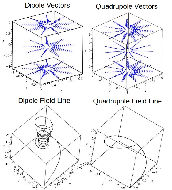
Figure 1: We show the dipole at left and quadrupole at right in this figure, both above and below the plane. At upper left the local field direction is shown in 3d for the dipole solution with only the sub scale turbulent helicity of Eqn. 9 present. The similarity class $a=1$ ,and the length unit is the radius of the disc. The spiral twist is very small except near the axis. The field line at lower left is for the dipole solution. It begins very near the axis at a large height above the disc and descends while spiralling rapidly to the point $\{r,\phi,z\}=\{0.22,0,0.5\}$. Note that the azimuthal field changes direction at large height. On the right the quadrupole solution shows less structure. The spiralling is very slow even at small radius (note the scale in the lower right hand image) and the azimuthal field component does not change sign even at large heights. The quadrupole field line shown, starts at $\{r,\phi,z\}=\{0.5,0,0.5\}$ and rises. Both of these field lines are shown in clusters in figure (2).

Figure 1 demonstrates that, unless one is very near the galactic axis, the spirally rising field lines are very open. The dipole solution shows some interesting structure with height because near the axis the vertical and azimuthal field components go through zero and reverse direction on the same side of the disc. Normally referred to as a ‘parity change’. The field line at lower left is shown descending from large height, but this is not necessary. The dipole field line ensemble in Figure 2 begins at $z=1.8$. The quadrupole solution at upper right of Figure 1 is a slowly rising spiral. The single field line is assembled in a cluster spaced around a circle in Figure 2, the different lines corresponding to different colours. Only close to the axis does the quadrupole show ‘X field’ behaviour in the $\{r,z\}$ plane. However the dipole solution shows a strong ‘X field’ throughout each quadrant. These poloidal projections are shown in Figure 3 below.

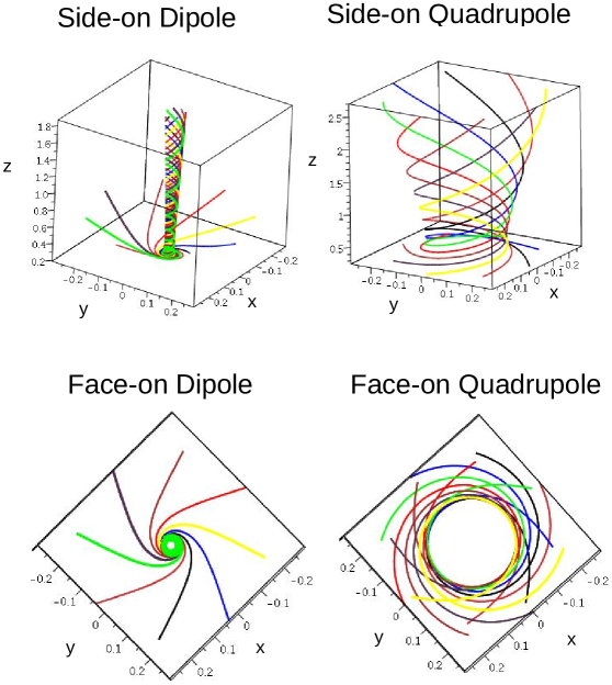
Figure 2: The left column shows a collection of field lines for the dipole and the right column show the quadrupole. The top row shows a side view and the bottom row shows a face-on view (the $\{r,\phi\}$ projection). For the dipole, the lines begin on a circle of radius $r=0.22$ at height $z=0.5$ and they are spaced at $45^{\circ}$ around the circle. The field lines are descending on the central ‘funnel’ and rising at large radius. One of these field lines (top left) is shown at lower left in figure (1) for clarity. The rising field lines indicate the connections between the outer vectors at upper left in figure (1). For the quadrupole, The field lines stand on radius $r=0.25$ at a height of $0.25$. They are spaced at $45^{\circ}$ around the circle and are rising.

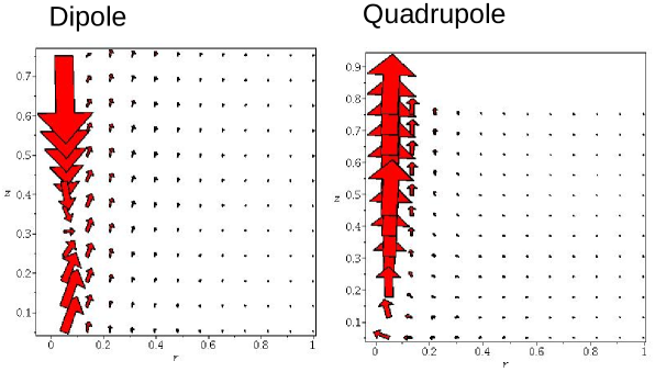
Figure 3: The left figure shows the pure $\alpha_{h}$ dynamo dipole in an $\{r,z\}$ cut. The right figure shows the pure $\{\alpha_{h}\}$ quadrupole in an $\{r,z\}$ cut. The only parameter is $\tilde{\alpha}_{h}$ which appears only in the evolution time scale. It does not affect the field topology.

Figure 3 shows the $\{r,z\}$ cuts through the upper half of the upper row images of Figure 1. These figures correspond to the images in Figure 2. Only the dipole shows a convincing high latitude ‘X field’ in projection. The axial behaviour of the magnetic fields shows the field coming down at $z>\sim 0.3$, and then rising at larger radii. At the same radius below $z\sim 0.3$, the field is rising as part of a field that descended at smaller radii.

The quadrupole image on the right shows magnetic field parallel to the disc plus an axial rising (inside $r\sim 0.15$) magnetic field. We should recall Eqn. 9 at this point, which indicates that the true sub scale turbulent vorticity goes as $\tilde{\alpha}_{h}\delta re^{-\alpha T}$. When $K=a=1$, $\alpha=\delta$, and the quantity $\delta r$ is generally set so as to give a macroscopic velocity in order of magnitude. That leaves $\tilde{\alpha}_{h}$ to determine the magnitude of the alpha effect.

One can only expect the pure $\alpha_{h}$ dynamo in galaxies for which there is little evidence of macroscopic jets or winds (unless the flow is parallel to the magnetic field). The macroscopic ($\alpha/\Omega$) dynamo in our model occurs either due to the lagging rotation in the halo or because of a gradient in the outflow/inflow velocities. There are essentially no parameters in the magnetic field of this section beyond the choice of the self similar class, $a$, which we have set equal to $1$ , reflecting a constant global velocity. This encourages us to search for this coherent magnetic field behaviour in the observations. One might expect this behaviour to be correlated with vigorous star formation.

Referring to the observed fields displayed in the CHANG-ES catalogue of Krause, Irwin, Schmidt et al. (2020), NGC 3044 may be a candidate for a pure star formation (i.e. sub scale turbulence resulting in $\alpha_{h}$) dynamo (see top of Figure 4 and the figures of this section). The base function would be predominantly dipole. The characteristic magnetic behaviour is observed to be predominantly high-latitude ‘X field’ with no parallel equatorial component. Moreover the field falls off rapidly radially but extends far into the halo. The very strong axial field is a formal feature of Eqn. 3 when $\alpha_{h}\rightarrow 0$ as $r\rightarrow 0$, because the spatial gradient times $\alpha_{h}$ is required to match the time derivative. There is also the $1/r$ field dependence that reflects the self-similar global symmetry. Figures 1, 2 and 3 all illustrate these properties for the $\alpha_{h}$ dipole.

The rotation measure (RM) given in Krause, Irwin, Schmidt et al. (2020) and displayed in rudimentary form by contours in Figure 4 varies as might be expected from rising, spiralling, field lines. In between the double-lines in the galaxy figures (solid and dashed curves close to each other) is where the RM sign changes. On the solid curve side, the RM is positive (field lines pointing towards us) and on the dashed curve side, the RM is negative (field lines pointing away from us). The RM also shows a sign change across the disc in some regions which can correspond to a change in sign of radial field. Figures 9 and 10 below show that the $\alpha_{h}$ dynamo with wind or even pure flux freezing with wind may also fit the data. NGC 3448 (not shown) may be a more depolarized second example.

NGC 3556 is another extreme where a coherent galactic field is scarcely established. It is likely that it is dominated by a series of local dynamos driven by local star formation, so we are actually seeing the turbulent nature of sub scale vorticity. That is, there are multiple $\alpha_{h}$ dynamos acting. The data are shown for comparison in the bottom image of Figure 4.

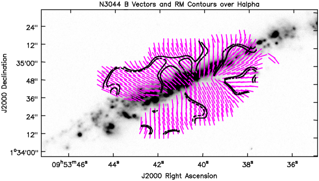
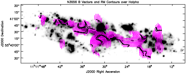
Figure 4: NGC 3044 (top) and NGC 3556 (bottom) with H$\alpha$ emission shown in greyscale. B vectors, corrected for Faraday rotation, are shown in magenta. RM contours have been set only for the purpose of indicating where there is a sign change from positive to negative or vice versa. The contours are set to +10 (solid curves) and -10 (dashed curves) rad m^-2 for NGC 3044 and at +15 (solid curves) and -15 (dashed curves) rad m^-2 for NGC 3556 to help guide the eye. That is, the sign change occurs in the narrow gap between the solid and dashed contours. See Krause, Irwin, Schmidt et al. (2020) for more explanation of the polarization data and Vargas et al. (2018) for information on the H$\alpha$ image. All data have been downloaded from queensu.ca/changes.

3.3 Halo rotational lag and the $\alpha_{h}$ dynamo

The general solution to Eqn. 19 with $v^{\prime}=-v_{1}$ for $\tilde{A}_{\Phi}(\zeta)$ becomes

$$\tilde{A}_{\Phi}(\zeta)=C1~{}(1+\zeta^{2})F(\alpha_{1},\beta_{1},\gamma_{1},-\zeta^{2})+C2~{}\zeta(1+\zeta^{2})F(\alpha_{2},\beta_{2},\gamma_{2},-\zeta^{2}),$$ (25)

where $F(\alpha,\beta,\gamma,z)$ is the hypergeometric function. The arguments are (with $n=1,2$)

$$\alpha_{n} = (\frac{3}{4}+\frac{n-1}{2})+\frac{\sqrt{1-4(K^{2}+v_{1})}}{4},$$

$$\beta_{n} = (\frac{3}{4}+\frac{n-1}{2})-\frac{\sqrt{1-4(K^{2}+v_{1})}}{4},$$ (26)

$$\gamma_{n} = \frac{1}{2}+(n-1).$$

In our examples the solution $\{C1,C2\}=\{1,0\}$ is ’dipolar’ in form with $b_{Z}$ non-zero at the disc, while the solution $\{C1,C2\}=\{0,1\}$ is quadrupolar and has zero $b_{Z}$ at the disc.

From Eqn. 9, we note that when $\tilde{\alpha}_{h}$ is constant we may use its value to define the sub scale turbulent velocity $<1$ and so let the velocity scale $\delta r$ be macroscopic. That is, $\delta r$ reflects mainly lagging rotational velocity $v$ or wind velocity $w$ (although we do not use a ‘wind’ velocity in this section). Consequently Eqn. 8 shows that the magnitude of $v$ and $w$ should be chosen $O(1/\tilde{\alpha}_{h})$ so as to reflect the larger macroscopic rotation and wind magnitudes. It is likely that $\tilde{\alpha}_{h}=O(0.1)$ (e.g. Tamburro et al., 2000) so that $v_{1}=O(1)$ (Heald et al., 2007) and $w_{o}$ and $w_{1}$ may be $O(10)$ in extreme cases (e.g. Heesen et al., 2018). Extensive supernova activity may lead to larger sub scale velocities locally.

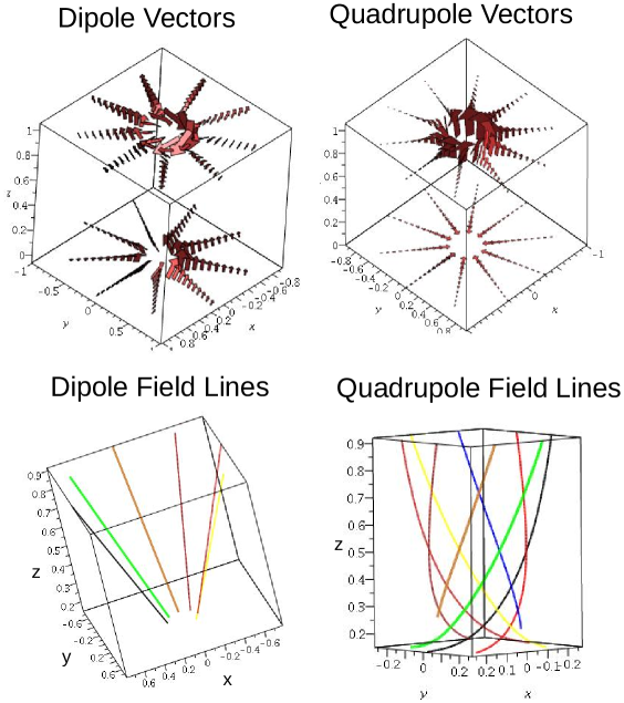
Figure 5: The top row shows the magnetic vectors in 3d for the dipole on the left and the quadrupole on the right. The bottom row shows clusters of field lines for the dipole on the left and the quadrupole on the right. The field lines of the lower row start at $z=0.15$, $r=0.25$, and then in steps of $\pi/4$ around the circle indicated by different colours. Only half the circle is shown for clarity. The rotational lag rate is $v_{1}=1$, $K=a=1$ for all of these examples. For the magnetic field vectors of the top row, only two levels in $z$ are shown for clarity, but they may be connected by referring to the 3d images of the second row.

In Figure 5, we show a dipole solution and a quadrupole solution in 3d on the top row and a cluster of corresponding field lines for each case in the bottom row. We show only the upper half plane for clarity, but $b_{\Phi}$ and $b_{Z}$ change sign on crossing the disc in the quadrupole solution, while only $b_{R}$ does so in the dipole solution.

We see that the quadrupole solution produces a projected ‘X type’ geometry (recall the axial symmetry) at small polar angle that includes the axis, while the dipole solution produces the X geometry at much larger polar angles. The dipole field lines appear to be straight in this representation because the poloidal field is much larger than the toroidal field. However they do turn in azimuth as is shown in Figure 6.

The dipole has an interesting structure at large height where the field lines become tightly wound near the axis. The winding sense is opposite to the sense of the exterior winding, which implies that the azimuthal field passes through zero at some height and radius. This leads to a sign change in the RM with latitude that can be seen in an RM plot (Henriksen, Woodfinden and Irwin, 2018a), but we do not show this here for brevity.

The addition of rotational halo lag has not greatly changed the topology from that of the pure $\alpha_{h}$ dynamo as seen in Figures 2 and 3. The dipole solution changes the rotation sense at height near the axis but remains similar at large radius, showing a strong X field. The quadrupole field is less tightly wound in the presence of halo lag and shows ‘X field’ only in a very limited range of latitudes. At this point, X field magnetic topology favours very much a dipole symmetry across the galactic equator.

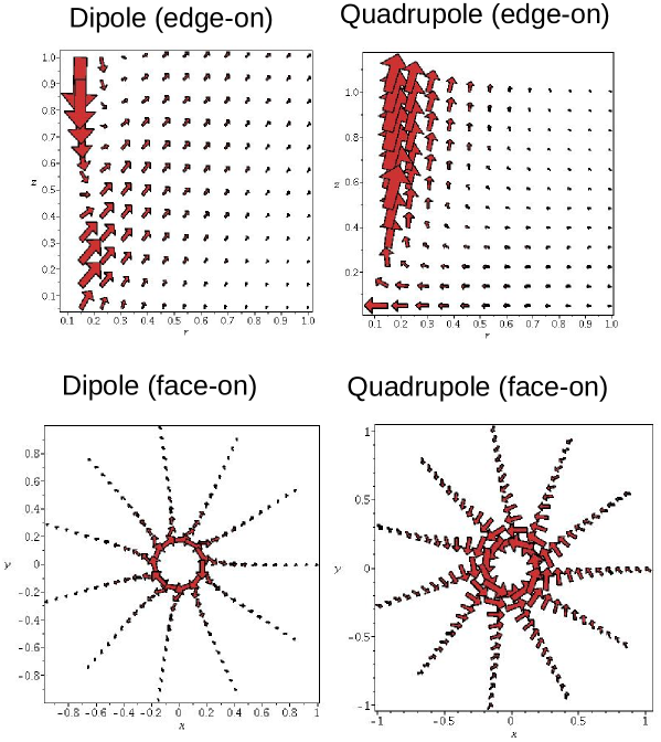
Figure 6: In the upper row, the left column shows the dipole magnetic field for the case $\{v_{1},K,C1,C2\}=\{1,1,1,0\}$ projected into the $\{r,z\}$ poloidal plane, integrated from $r=015$ and $z=0.05$. This contrasts the X field behaviour. The right column shows the same projection for the quadrupole solution with parameters $\{1,1,0,1\}$. The lower row shows the corresponding projections in the toroidal plane at $z=0.5$

Figure 6 shows poloidal and toroidal cuts of the same fields shown in Figure 5. The quadrupole solution shows very similar behaviour to the pure alpha solution although it is less tightly wound. The dipole solution has the very tight winding near the galactic axis as does the pure turbulent field and has a very strong X field behaviour generally. The sign of the pitch angle of the dipole magnetic field changes sign with height and radius. Such behaviour is more in accord with the average CHANG-ES behaviour, as shown in Krause, Irwin, Schmidt et al. (2020).

In terms of the observations reported in Krause, Irwin, Schmidt et al. (2020), Figures 6 and 3 show that it would be difficult to detect the effect of moderate halo rotational lag on the $\alpha_{h}$ dynamo for the dipole, except near the axis. However near the axis tight winding can lead to beam depolarization as for the dipole in Figure 5. This often seems to be the case observationally. The quadrupole does not deliver a convincing X field.

We turn in the next section to a similar study of the magnetic effects of a combined accelerating wind and halo rotational lag.

3.4 Accelerating disc wind plus halo rotational lag acting on the turbulent dynamo

Given the (sub scale) turbulent dynamo with constant $\tilde{\alpha}_{h}$ plus either outflow or accretion and rotational halo lag, Eqns. 3 plus scale invariance lead to the equations for the scaled vector potential as

$$K\tilde{A}_{R} = -\tilde{A}_{\Phi}^{\prime}(1+\zeta v(\zeta))+v(\zeta)\tilde{A}_{\Phi}-w(\zeta)(\tilde{A}_{R}^{\prime}+\zeta\tilde{A}_{Z}^{\prime}),$$

$$K\tilde{A}_{\Phi} = \tilde{A}_{R}^{\prime}+\zeta\tilde{A}_{Z}^{\prime}-w(\zeta)\tilde{A}_{\Phi}^{\prime},$$ (27)

$$K\tilde{A}_{Z} = \tilde{A}_{\Phi}+(v(\zeta)-\zeta)\tilde{A}_{\Phi}^{\prime}.$$

These may be combined to give the equation for $\tilde{A}_{\Phi}$ as

$$(1+w(\zeta)^{2}+\zeta^{2})\tilde{A}_{\Phi}^{\prime\prime}+2w(\zeta)(K+w(\zeta)^{\prime})\tilde{A}_{\Phi}^{\prime}+(K(K+w(\zeta)^{\prime})-v(\zeta)^{\prime})\tilde{A}_{\Phi}=0.$$ (28)

The scaled magnetic field components are given as in Sect. 3.1. These can be expressed solely in terms of the azimuthal vector potential and its derivative plus the auxiliary velocities, by using Eqns. 27.

The forms for the auxiliary scaled vertical velocity and the scaled rotational lag (the physical velocity is given in Eqn. 8) are taken as

$$w(\zeta) = w_{o}+w_{1}\zeta,$$ (29)

$$v(\zeta) = -v_{1}\zeta,$$ (30)

where $w_{o}$ gives the scaled vertical velocity at the disc, $w_{1}$ is the scaled rate of acceleration with $\zeta$ and $v_{1}$ gives the scaled halo lag. If $w_{o}$ and $w_{1}$ are negative then we have an decelerating flow onto the disc. If $w_{1}>0$ with negative $w_{o}$ then we may have an accelerating inflow. The rotational lag rate $v_{1}$ is generally positive. One should note that near the axis of the galaxy $\zeta\rightarrow\infty$. Either scaled velocity is then singular above the nucleus, but the physical velocity (8) simply increases with height.

Eqn. 28 may now be solved in terms of hypergeometric functions with complicated arguments, according to MAPLE 2019. We proceed to express a few results for ‘typical’ parameters. In Figures 7 and 8.

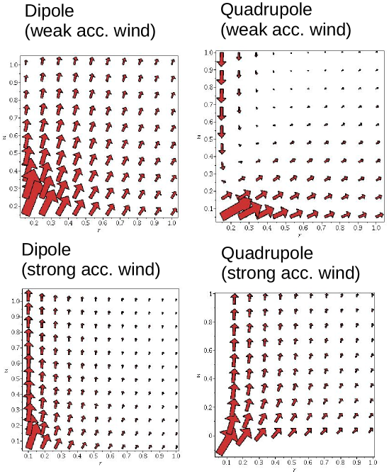
Figure 7: Here, the magnetic field is subject to a disc wind and vertical acceleration in an outflow in addition to sub scale turbulence. The left hand column shows the dipole field in the $\{r,z\}$ plane with parameter vector $\{v1,w_{o},w_{1},K,r,z,C_{1},C_{2}\}$ equal to $\{0,1,1,1,r,z,1,0\}$ at upper left (a weaker wind) and $\{0,1,3,1,r,z,1,0\}$ at lower left (a strong wind). The strong accelerating wind at lower left has pulled the field nearly parallel to the axis. The right column shows the quadrupole solution with parameter vector $\{0,1,1,1,r,z,0,1\}$ at upper right and $\{0,1,3,1,r,z,0,1\}$ at lower right. At lower right the magnetic field is rendered almost entirely vertical by a gradient in the vertical wind velocity.

In Figure 7, we show sample ‘dipole’ and ‘quadrupole’ magnetic fields with and without a strong wind acceleration. The cuts are in the $\{r,z\}$ plane and since the field is axially symmetric the $3d$ topology is easily inferred. The macroscopic motions act on the sub scale magnetic field that is present due to turbulence ($\alpha_{h}$ dynamo). The constant auxiliary function $\tilde{\alpha}_{h}$ does not appear in the equations except in the temporal evolutionary Eqn. 18. The magnetic topology is very sensitive to an accelerating wind velocity. Such a gradient generates an $\alpha_{h}/\Omega$ (macroscopic) dynamo just as a halo rotational lag or a gradient of angular velocity in the disc.

It is not shown here but we find that a strong disc wind ($w_{o}\leq\sim 10$) without strong acceleration only convects the boundary conditions at the disc to large heights, with little change in the topology. For this reason we have focussed on the acceleration in the examples.

What this figure emphasizes over all, is the strong dependence on the wind gradient of the magnetic topology in the halo with a moderate initial disc wind. The ‘quadrupole’ solution shows ‘X field’ structure only with the wind acceleration. The dipole field gives a strong ‘X field’, particularly without wind acceleration.

By varying the initial disc wind $w_{o}$ and the acceleration rate $w_{1}$, intermediate cases can be found. The field is also combed out by accelerating accretion because there is no barrier at the disc in the model. Decelerating accretion can be arranged with both $w_{o}$ and $w_{1}$ negative.

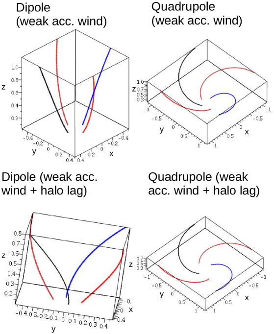
Figure 8: All the field lines in different panels of this figure are started at $r=z=0.25$ and $\phi=0$. At upper left, a cluster of field lines for a dipole case is shown taken from the image at upper left in figure(7). The parameter set is $\{v1,w_{o},w_{1},K,r,\phi,z,C_{1},C_{2}\}$ = $\{0,1,1,1,r,\phi,z,1,0\}$. The lower left panel is for a dipole with parameter set $\{1,1,1,1,r,\phi,z,1,0\}$. The field lines are placed at cardinal points around the initial circle and height. At upper right, four quadrupole field lines that are taken from the $\{r,x\}$ image at upper right in figure (7) are shown. The parameter list is $\{0,1,1,1,r,\phi,z,0,1\}$ for the quadrupole at upper right. The lower right cluster is for a quadrupole magnetic field with the parameter set $\{1,1,1,1,r,\phi,z,0,1\}$.

The quadrupole column in Figure 8 compares a moderate accelerating wind with no halo rotational lag (upper panel) to one with a halo rotational lag, comparable to the accelerating wind velocity at the disc. The flatter spiral generation with the presence of halo lag is quite marked, because the lines in the lower panel rise only to a height of $0.7$ rather than $\sim 1$. We recall that the unit of length is the radius of the galactic disc.

A similar flattening effect is observed with the same change in rotational halo lag for the dipole, as shown in the left hand column panels. Because it appears (Figure 7) that the dipole is the principal source of strong X fields, we can recognize the effects of halo lag in the increasing polar angle (decreasing halo latitude) of the magnetic polarization with increasing lag rate.

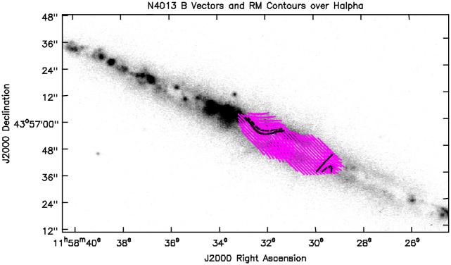
Figure 9: The image shows NGC 4013 with H$\alpha$ emission shown in greyscale. B vectors, corrected for Faraday rotation, are shown in magenta. RM contours have been set only for the purpose of indicating where there is a sign change from positive to negative or vice versa, and are present to help guide the eye. The contours are set to +10 (solid curves) and -10 (dashed curves) rad m^-2 See Krause, Irwin, Schmidt et al. (2020) for more explanation of the polarization data and Vargas et al. (2018) for information on the H$\alpha$ image. All data have been downloaded from queensu.ca/changes.

Adding a halo rotational lag adds to the complexity of the magnetic topology. In particular it can lead most noticeably to a reversal of the magnetic helicity with height, which leads to the observed reversal in ‘parity’ in the RM. This is similar to the behaviour found in Henriksen & Irwin (2016). The lag also increases the extent of the projected ‘X field’ near the disc.

Figure 9 shows the CHANG-ES polarization (with Faraday Depth sign change) data for the galaxy NGC 4013. The X magnetic field is wound very tightly and is really only visible very close to the disc. This might suggest, according to Figures 7 and 8, that the coherent magnetic field in NGC 4013 is a quadrupole with considerable halo rotational lag. However, close inspection of Figure 9 reveals that the field is more like an inverted V than an X. That is, the field converges on the axis above the disc. There is weak indication of this for the quadrupole in Figure 6.

We conclude from this section that a vigorous constant wind can carry equatorial boundary conditions to large heights. However a gradient in the wind velocity is more important for the magnetic complexity such as strong deviations from a pure $\alpha_{h}$ dynamo. The main effect of a strong wind is to transport magnetic field to greater height and to remove the ‘X field’ in favour of a poloidal field perpendicular to the galactic disc. The behaviour is particularly pronounced near the axis. The rotational halo lag along with the wind acceleration, acts as an $\alpha/\Omega$ dynamo given the $\alpha_{h}$ sub scale turbulent average dynamo. The rotational lag gives a field strongly wound near the disc while the wind acceleration stretches the field vertically.

Reviewing the observations in the CHANG-ES catalog, we note that NGC 3044 (top of Figure 4) may be compatible with a moderate disc wind and acceleration as seen for the dipole in Figure 7 at upper right. This is more consistent with the extended halo in NGC 3044 than is the pure $\alpha_{h}$ dynamo of Sect. 3.2.

Quadrupole behaviour seems rarer but may be illustrated in NGC 4013 (Figure 9). We refer to both the CHANG-ES catalog (Krause, Irwin, Schmidt et al., 2020) and Figure 12 in Stein et al. (2019). At upper right in Figure 7, we see a quadrupole with field largely parallel to the disc (i.e. a very low latitude X field) that falls off rapidly into the halo. The model predicts therefore large angle but weak X field, which corresponds to Figure 12 in Stein et al. (2019). The data from Krause, Irwin, Schmidt et al. (2020) is shown in Figure 9. The sign change in the RM across the disc in NGC 4013 can also be due to a quadrupole.

3.5 A pure macroscopic ‘dynamo’

We consider the special case when there is no active $\alpha_{h}$ effect combined with macroscopic motion, as there has been in all previous cases. It should be described nevertheless as an $\alpha/\Omega$ dynamo because there must be an initial field for the velocity to act on. With $a=1$ and $K=1$, flux density is conserved (equivalent Dimensionally to a magnetic field or velocity constant) and a local field grows linearly according to Sect. 2.1.

The existence of a global magnetic flux constant requires $a=3$ and hence $K=-1$. Global flux conservation can only produce topological enhancements in the magnetic field which will decline slowly in time. We recall the discussion of time dependence in Sect. 2.1, which shows the magnetic field to decrease in time as $(1+\alpha t)^{-1/3}$ with $a=3$.

We set $\tilde{\alpha}_{h}=0$ in this section and so Eqn. 7 defines the logarithmic time. Because we also suppress the diffusion in this paper, we are left with the pure flux freezing during the macroscopic motion as described by the second term in Eqn. 3. We continue with our scale invariant formulation, which prescribes the velocity field according to Eqn. 8 and the magnetic field according to Eqns. 10 and 13. We proceed with only rotational and outflow/inflow velocities so that the radial velocity $u=0$. This limit is related to the study performed in Henriksen & Irwin (2016) using dynamical equipartition and a Mestel disc, but here the assumption of scale invariance dictates the velocity field, rather than a dynamical model.

The reason for studying this limiting case is due to the predictive nature of the analytic magnetic fields with regard to scale heights of the magnetic field. This is related to the recent results for CHANG-ES galaxies reported in Krause, Irwin, Wiegert et al. (2018).

The surviving term in Eqn. 3 requires solving a simple set of equations for the scale invariant vector potential namely

$$K\tilde{A}_{R} = v(\tilde{A}_{\Phi}-\zeta\tilde{A}_{\Phi}^{\prime})-w(\tilde{A}_{R}^{\prime}+\zeta\tilde{A}_{z}^{\prime}),$$

$$K\tilde{A}_{\Phi} = -w\tilde{A}_{\Phi}^{\prime},$$ (31)

$$K\tilde{A}_{Z} = v\tilde{A}_{\Phi}^{\prime}.$$

Note that it is the outflow/accretion that drives the whole system. Setting $w=0$ renders the system trivial.

Eqns. 31 are easily solved analytically when we take the halo rotational lag in the pattern frame and the outflow velocity in the familiar forms

$$v = -v_{1}\zeta,$$

$$w = w_{o}+w_{1}\zeta,$$ (32)

However even the case, wherein $v$ and $w$ are both constant (so that physical velocities are proportional to $r$ from Eqn. 8, is of interest as it is both analytic and simple. The field components follow ultimately from Eqns. 22 to 24. These imply with $v$ and $w$ constant and Eqns. 31, that

$$b_{R} = -\frac{e^{(2\delta-\alpha)T}}{rw}KC_{1}e^{-\frac{K}{w}\frac{z}{r}},$$

$$b_{\Phi} = \frac{e^{(2\delta-\alpha)T}}{rw}e^{-\frac{K}{w}\frac{z}{r}}(C_{1}v-C_{2}K),$$ (33)

$$b_{Z} = \frac{e^{(2\delta-\alpha)T}}{r}C_{1}e^{-\frac{K}{w}\frac{z}{r}}(1+\frac{K}{w}\zeta).$$

From these relations we observe that the exponential decline of the magnetic field in $z$ at fixed $r$, is slower with larger wind velocity, so that the scale height increases. The exponential decline is also slower at larger $r$ for a constant outflow, which gives the magnetic (or radio) halo a ‘butterfly’ shape. The azimuthal field increases with increasing $v$ and decreases with increasing $w$ at the disc. The radial field also decreases with increasing $w$ at the disc. Boundary conditions at the disc are ‘lifted’ into the halo. This behaviour has also been found in the previous section.

In general, an individual field line always extends in the same sense in radius, azimuth, and height so that it appears as a rising, expanding helix, much as shown in Henriksen & Irwin (2016). It differs from the pure $\alpha_{h}$ dynamo of the Sect. 3.2, in that the spirals are detectable at much larger radii. This topology already gives an X type field near the disc when projected into the $\{r,z\}$ plane.

We note from the solution that $b_{R}$ changes sign with $w$ on crossing the disc. However there is no halo rotational lag in $z$ with $v$ constant, but there is in radius by Eqn. 8. Therefore there is no need for $v$ to change sign on crossing the disc. Moreover $b_{\Phi}$ also changes sign on crossing the disc. The component $b_{Z}$ does not change sign because $\zeta$ also changes sign. Thus the field obeys a dipole symmetry, but with a change in sign of both tangential field components.

As a result of these symmetries, there is a change in the magnetic helicity on crossing the disc. The term in $C_{2}$ comes from the homogeneous part of the equation so we normally set it equal to zero. It would be necessary in order to confront a specified boundary condition. The only quadrupole type solution is with $C_{1}=0$, which gives only a purely azimuthal field, possibly discontinuous at the disc

When the outflow and lag functions have the forms of Eqns. 32, rather than being constant, the solution for the field becomes

$$b_{R} = \frac{e^{(2\delta-\alpha)T}}{rw(\zeta)}K\tilde{A}_{\Phi}(\zeta),$$

$$b_{\Phi} = -\frac{e^{(2\delta-\alpha)T}}{rw(\zeta)}\big{(}\zeta v_{1}(1+\frac{K\zeta}{w(\zeta)})-\frac{Kv_{1}}{w_{1}}(\zeta+\frac{w_{o}}{w_{1}}\ln{w(\zeta)})+KC_{2}/C_{1}\big{)}\tilde{A}_{\Phi}(\zeta),$$ (34)

$$b_{Z} = \frac{e^{(2\delta-\alpha)T}}{r}(1+\frac{K}{w}\zeta)\tilde{A}_{\Phi}(\zeta).$$

The azimuthal vector potential has the power law form

$$\tilde{A}_{\Phi}=C_{1}e^{-\frac{K}{w_{1}}\ln{w(\zeta)}}.$$ (35)

In these formulae $w_{1}\neq 0$ and, if $w_{o}=0$, there is a logarithmic singularity at $\zeta=0$. Once again the general behaviour is that of a rising, widening, spiral as was first seen in Henriksen & Irwin (2016). On crossing the equator, we might expect $w_{o}$ and $v_{1}$ to change sign, but not $w_{1}$ so that $w$ changes sign. Hence $b_{R}$, $b_{\phi}$ change sign but $b_{z}$ does not, implying dipole behaviour as in the constant velocity case. We intend the real part of the logarithm in these expressions.

We append a relatively generic example in Figure 10 in order to fix ideas. Depending mainly on the relative size of the halo lag $v_{1}$ relative to the wind acceleration, $w_{1}$ the spirals are flatter when the ratio is large and more extended when the ratio is small. Recall that the Unit in the figures is the disc radius. The constant wind velocity merely convects boundary conditions as we have seen before. This is because it does not contribute to a differential twisting of the field.

The ‘X type’ field behaviour is found in projection as a characteristic of rising, spiralling fields. It will be at an angle close to the disc when the halo lag rate is dominant and closer to the galactic axis when the wind acceleration is stronger. A strong wind acceleration case (not shown) has almost straight field lines in the halo rather than flatly spiralling field lines. This is very similar to the quadrupole $\alpha_{h}$ behaviour.

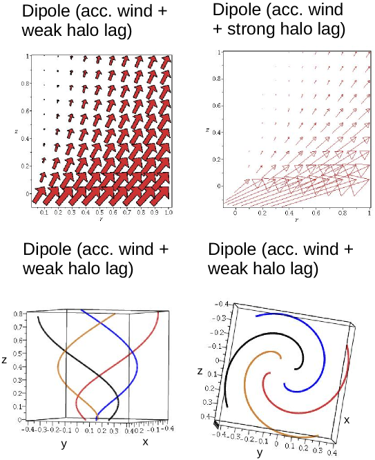
Figure 10: In the bottom row we show a cluster of 3D field lines for the parameters $\{v_{1},w_{o},w_{1},K,C_{1},C_{2}\}=\{0.15,1.0,0.1,1,1,0\}$. The field lines all pass through $r_{o}=0.25$, $z_{o}=0.25$ and through the cardinal points on the circle of radius $r_{o}$. The side view is on the left and the top view is on the right. There is no true quadrupole as can be seen from Eqns. 34 and 35. The plot in the $\{r,z\}$ plane at upper left is for the same parameters. The plot at upper right shows the effect of a strong halo rotational lag with parameters $\{1,0.25,0.25,1,1,0\}$. The arrows correspond to values at their head.

We summarize this section by comparing it to the pure $\alpha_{h}$ dynamo of Sect. 3.2. We have found widening, spiralling, halo structure in both limits as elaborated below.

The pure $\alpha_{h}$ sub scale turbulent average dynamo produces tightly wound spirals near the axis of the galaxy, where they are unlikely to be observed. The large radius spirals are very slow and the projections into the $\{r,z\}$ plane show ‘X type’ topology only near the disc for the quadrupole solution. The dipole $\alpha_{h}$ solution shows a rapid decline in field strength with height in the azimuthal and vertical field components when the lag and wind are weak.

The macroscopic flux freezing scale invariant dynamo of the present section produces rising spiral magnetic fields with large polar angle, when the halo rotational lag velocity dominates the wind velocity. The X type topology is then projected into the $\{r,z\}$ plane in a well defined low latitude sector. The wind dominated case shown at upper left gives a more typical X field topology. There is also scope for varying the sign of the Faraday depth above the disc when the spirals are rapidly turning inside the galactic halo. This is especially likely when the halo rotational lag dominates.

Referring once more to Krause, Irwin, Schmidt et al. (2020), The flux freezing ‘dynamo’ alone can not give both a high latitude X field and a parallel field in the disc. However it shows clearly the association between the X field topology and rising magnetic spirals. The wind dominated field is a natural explanation for the observed magnetic topology in NGC 3044 (see Figure 4).

The C band image of NGC 4631 indicates similar poloidal behaviour, but the multiple sign changes in RM in this galaxy suggests the presence of non axially symmetric spiral arms (see e.g. Woodfinden et al., 2019) in the halo.

3.6 Latitude dependence of sub scale turbulence and rotational halo lag

We turn to consider a sub scale turbulent dynamo varying with latitude and acted on by a rotationally lagging halo. That is, we allow the auxiliary turbulent quantity $\tilde{\alpha}_{h}$ to be a function of $\zeta\equiv z/r$. By concentrating the scaled sub scale turbulent helicity to the galactic axis in this way, we imitate the effect that an AGN may have on the global galactic magnetic field. The effects of an axial wind must be left to another work.

The suggestion of an axially symmetric ‘AGN dynamo’ assumes that the AGN axis is approximately aligned with the axis of the galaxy. In galaxies where this is not the case we can expect more asymmetric galactic magnetic fields, at least near the nucleus. It is not necessary for a galaxy to have an axial concentration of magnetic field, such as may be produced by an AGN, in order to display a large scale coherent magnetic field. We have seen this in previous sections, especially with the quadrupole mode where the field may be tightly wound about the axis.

If we choose $\tilde{\alpha}_{h}$ to be linear in the tangent of the latitude, $\zeta$, according to

$$\tilde{\alpha}_{h}=\alpha_{h1}\zeta,$$ (36)

then we must use $T$ as defined in Eqn. 7. Consequently, the constant $\tilde{\alpha}_{h1}$ no longer vanishes from the equations for the vector potential.

We have, with Eqn. 36, assumed (recalling Eqn. 9) that the physical sub scale turbulent helicity increases linearly with height in the halo. However the scale invariant solution may be expected to react to the latitude dependence in $\tilde{\alpha}_{h}$. The linear form satisfies the antisymmetry across the disc (e.g. Klein & Fletcher, 2015).

This form for $\tilde{\alpha}_{h}$ parallels the assumption regarding the form of the halo rotational lag (see Eqn. 14) relative to a pattern frame. In fact if we assume that our calculation is done in a uniformly rotating ($\Omega$) pattern frame, we can associate $2\Omega r$ with the base hydrodynamic vorticity to which we add the value (Eqn. 36).

Eqns. 3 for the components of the vector potential become, when $\tilde{\alpha}_{h}$ varies generally with $\zeta$,

$$K\tilde{A}_{R} = -\tilde{\alpha}_{h}(\zeta)\tilde{A}_{\Phi}^{\prime}+v\tilde{A}_{\Phi}-\zeta v\tilde{A}_{\Phi}^{\prime},$$

$$K\tilde{A}_{\Phi} = \tilde{\alpha}_{h}(\zeta)(\tilde{A}_{R}^{\prime}+\zeta\tilde{A}_{Z}^{\prime}),$$ (37)

$$K\tilde{A}_{Z} = \tilde{\alpha}_{h}(\zeta)(\tilde{A}_{\Phi}-\zeta\tilde{A}_{\Phi}^{\prime})+v\tilde{A}_{\Phi}^{\prime},$$

and these combine to give the equation for the azimuthal vector component. Once this equation is solved the other components and the magnetic field components follow. The equation to be solved takes the general form

$$(1+\zeta^{2})\tilde{A}_{\Phi}^{\prime\prime}+\frac{d\ln{\tilde{\alpha}_{h}(\zeta)}}{d\zeta}(1+\zeta^{2})\tilde{A}_{\Phi}^{\prime}+(\frac{K^{2}}{\tilde{\alpha}_{h}(\zeta)^{2}}-\zeta\frac{d\ln{\tilde{\alpha}_{h}(\zeta)}}{d\zeta}-v^{\prime})\tilde{A}_{\Phi}=0.$$ (38)

Using Eqns. 36 and Eqn. 14, this last equation simplifies to

$$(1+\zeta^{2})\tilde{A}_{\Phi}^{\prime\prime}+(\zeta+\frac{1}{\zeta})\tilde{A}_{\Phi}^{\prime}+(\frac{K^{2}}{\alpha_{h1}^{2}\zeta^{2}}-1+v_{1})\tilde{A}_{\Phi}=0.$$ (39)

This equation has a logarithmic singular point at $\zeta=0$. However in the limit $\zeta\rightarrow 0$ the solution is proportional to $\zeta^{p}$ where $p^{2}=-K^{2}/\alpha_{h1}^{2}$. Consequently the singularity is an oscillation in $\ln{\zeta}$ and is easily recognized as $\alpha_{h1}\rightarrow 0$. We observe in our examples below that this oscillation is associated with the sub scale turbulence becoming dominant, as it extends to smaller scales.

The magnetic field is no longer invariant under a change in sign of $\zeta$ according to Eqn. 39 because of the term in $v_{1}$, which changes sign on crossing the disc. The sign of $\alpha_{h1}$ is irrelevant as one might expect because only the magnitude of the vorticity should produce the alpha dynamo.

A solution of Eqn. 39 at positive $\zeta$ can be pasted into the negative region (keeping the sign of $\tilde{A}_{\Phi}$ unchanged, but remembering to change the sign of $v_{1}$) to establish symmetry. This yields, by Eqns. 37 and the equations for ${\bf b}$, a change in sign of $b_{R}$ and $b_{\Phi}$ but not in $b_{Z}$. This would construct local dipole boundary conditions, but a quadrupole boundary follows by changing the sign of $\tilde{A}_{\Phi}$. However the oscillations in sign near the disc due to small scale turbulence confuse the issue. These fluctuations become smoothed to a coherent quadrupole for the $\{0,1\}$ solution, and to a coherent dipole for the $\{1,0\}$ solution when $v_{1}=\alpha_{h1}=O(1)$.

We observe, from Eqns. 8 and 9, that if indeed $\tilde{\alpha}_{h}=\alpha_{h1}\zeta$, and $v=-v_{1}\zeta$, then

$$v_{s}=-\delta rv_{1}\zeta e^{(-\alpha)T}~{}~{}~{}~{}~{}~{}\alpha_{h}=\alpha_{h1}\zeta e^{(-\alpha T)}.$$ (40)

It is convenient to choose $\delta r$ to be the actual lag rate so that $v_{1}=O(1)$. This means that the value of $\alpha_{h1}$ is likely to be also $O(1)$.

The magnetic field components take the same form as in Sect. 3.1 except for $\bar{b}_{\Phi}$. Eqn. 23 becomes, using the expression for $\bar{A}_{\Phi}$ in Eqn. 37 divided by $\tilde{\alpha}_{h}(\zeta)$,

$$\tilde{b}_{\Phi}=\frac{K\tilde{A}_{\Phi}}{\tilde{\alpha}_{h}(\zeta)}.$$ (41)

Recalling the linear form $\tilde{\alpha}_{h}$ (Eqn. 36) we see that the sign of $\alpha_{h1}$ affects the sign of $\tilde{b}_{\Phi}$ as one expects from helical (vortical) turbulence, but it does not affect the magnetic topology.

3.6.1 Examples

The two independent solutions of Eqn. 39 ($\{C_{1},C_{2}\}=\{0,1\}$ or $\{1,0\}$) are complex conjugates. We choose the real part of the $\{0,1\}$ solution and the imaginary part of the $\{1,0\}$ solution. This is because these choices best fit the expected quadrupole and dipole boundary conditions.

The oscillatory logarithmic singularity at small $\zeta$ is quite obvious in the solutions for small $\alpha_{h1}$ near the disc for small values of $\alpha_{h1}$. This is formally because whenever $K^{2}/\alpha_{h1}^{2}$ dominates the factor of $\tilde{A}_{\phi}$ in Eqn. 39, the oscillatory approximation extends to larger $\zeta$. However $\zeta$ must still be less than one (polar angle greater than $45^{\circ}$), so that the oscillations occur near the galactic disc. Physically, this is of interest because the $\alpha_{h}$ term in Eqn. 3 is due to sub scale turbulence. As this term becomes dominant at smaller scales (i.e. smaller $z$ at fixed $r$) , we can expect turbulence to manifest itself in the magnetic field.

The $\{r,z\}$ plane for the $\{0,1\}$ (quadrupole) solution is shown at upper right in Figure 11 and some corresponding field lines are shown at lower right. The field lines are constrained to the same scales on each axis. The images in the left column of the figure are for the $\{1,0\}$ (dipole) solution. Strong field lines descend rapidly near the axis and then rise. The ‘X type’ projected field lines are confined to a range of latitude near $45^{\circ}$ Latitude.

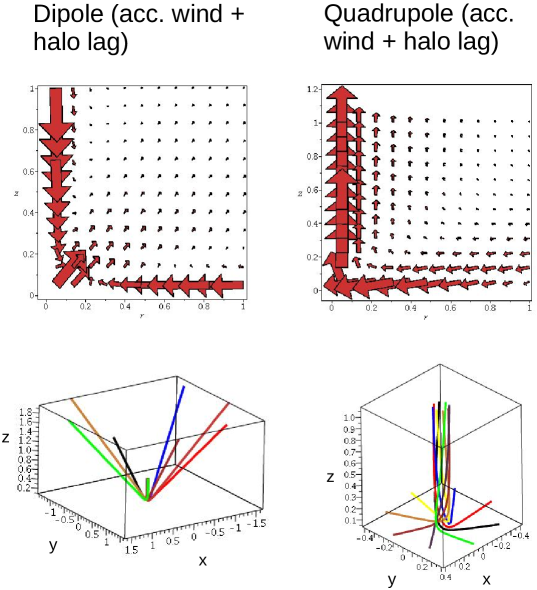
Figure 11: In the left column, we show the dipole with parameters $\{v_{1},\alpha_{h1},K,r,z,C_{1},C_{2}\}=\{1,1,1,r,z,1,0\}$. The $\{r,z\}$ plane is on the top and a cluster of field lines is on the bottom. All field lines in this figure pass through $r=0.05$ and $z=0.1$ and are distributed in steps of $\pi/4$ in azimuth. The $\{r,z\}$ cuts must be imagined rotated about the axis and the field line plots are filled in by similar field lines. The right column illustrates, in the same manner, the quadrupole with parameters $\{1,1,1,r,z,0,1\}$.

One should remember that in all mages of the $\{r,z\}$ plane the diagonal, apparently rectilinear magnetic vectors, are actually turning in the $\{r,\phi\}$ plane. Thus they represent rising or falling spirals as confirmed in Figure 12. The twist rate differs depending on the parameters and frequently varies with height above the disc and radius in the disc.

The quadrupole behaviour is strongest parallel to the axis and also parallel to the equator. The transition in field direction occurs near $45^{\circ}$ and removes any X type topology in favour of a nearly vertical field at large latitude. The corresponding field lines in the lower right panel illustrate that the field near the axis is nearly vertical with small toroidal field. The upper right panel shows how field lines starting at higher latitude fill the space of the lower panel.

The dipole behaviour in the left column of Figure 11 has a descending strong vertical field near the axis that rises almost rectilinearly, as seen in the field lines in the lower panel. These produce the X field topology near $45^{\circ}$. The toroidal plot in Figure 12 indicates only a very small azimuthal field compared to the quadrupole. These figures are for nearly equal lag velocity and sub scale turbulent velocity.

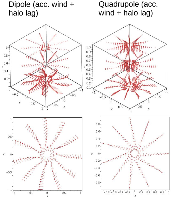
Figure 12: The figure at upper left is the 3d version of the case shown in the left column of figure (11). The parameters are the same $\{v_{1},\alpha_{h1},K,r,phi,z,C_{1},C_{2}\}=\{1,1,1,r,phi,z,1,0\}$. The right column has the parameter set $\{1,1,1,r,phi,z,0,1\}$ and corresponds to the right column in figure (11). The lower panels show an $\{r,\phi\}$ toroidal projection at height $z=0.25$ in each case for the same prameters.

Figure 12 shows, at upper right, the $3d$ version of the $\{r,z\}$ cut at upper right in Figure 11. The toroidal cut of the same field is shown at lower right. The field lines descend from the halo at large radius and then rise again at latitudes greater than $\pi/4$. The very slight toroidal field near the axis compared to the vertical field is shown in the lower right panel.

At upper left in Figure 12, we have the $3d$ image of the dipole with the same parameters. The field lines descend while turning slowly and subsequently rise rectilinearly at larger radius. This develops in a self similar fashion from all heights. The transition region contains a projected ‘X field’ to be present mainly near $45^{\circ}$. The azimuthal components of the vectors change sign with radius.

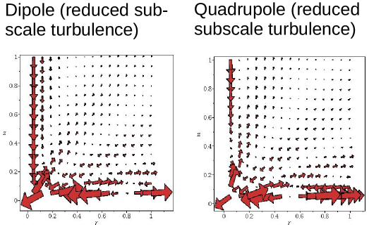
Figure 13: The image at left shows the $\{r,z\}$ field line vectors for the dipole case $\{v_{1},\alpha_{h1},K,r,\phi,z,C_{1},C_{2}\}=\{1,0.25,1,,r,\phi,z,1,0\}$. At right we have the quadrupole field line vectors with parameter set $\{1,0.25,1,r,\phi,z,0,1\}$. These reveal the onset of galactic disc small scale magnetic turbulence.

In Figure 13, we show the effects of reducing the scale and strength of the sub scale turbulence. The halo rotational lag has been kept constant but $\tilde{\alpha}_{h1}=0.25$ in both the quadrupole and dipole panels. Both modes now show X field topology in two narrow but separated sectors. The quadrupole actually shows three X field sectors, but one is very close to the equator of the galaxy. The more interesting development is the increasing turbulence in the disc of the galaxy for both modes. This tendency increases in latitude extent as $\tilde{\alpha}_{h1}$ decreases further.

This small scale turbulence is to be expected when the alpha dynamo dominates. Its appearance actually represents a confirmation of the form for this sub scale dynamo, as used in the classical Eqn. 3.

An interesting result of this section is the appearance in the dipole of strong axial magnetic field, together with X field topology that is intermediate between the axis and the equator. Although we have not included a ‘jet’ or a nuclear ‘wind’ directly, the dipole produces an axial field that we know from previous sections would not be changed by a constant vertical outflow velocity required in a jet or wind. This is achieved this by assuming a strong source of scaled sub scale vorticity on the galactic axis. This can be produced by an AGN, that is, by a super massive black hole or a burst of star formation. Such nuclear flows may therefore be an important contributor to the global galactic magnetic field.

If jets or nuclear star bursts do contribute to the coherent galactic magnetic field, we can expect a correlation between the presence of a galactic AGN and the strength of the magnetic field. In fact the disc field is also strong and turbulent (see Figure 13). Both the correlation and the turbulence would indicate an important sub scale dynamo. Similar global magnetic topology can be produced without an AGN but the strong axial field will be absent. This prediction may be readily tested for galaxies where the AGN axis and galactic axis coincide.

Perhaps the best candidates from CHANG-ES results are NGC 4388 and NGC 3079. Recent images of these two galaxies are shown in Figure 14. There is indeed a correlation between the strength of the coherent galactic polarization and the presence of AGN activity as a nuclear wind. The RM sign changes in NGC 4388 tend to indicate spiralling fields above the disc. This is less clear in NGC 3079 but also present. NGC 4388 shows rapid changes in field direction in the disc region, which may be turbulent.

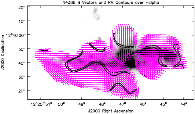
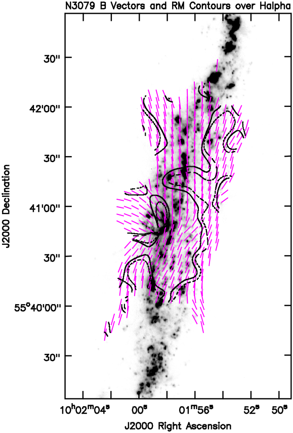
Figure 14: NGC 4388 (left) and NGC 3079 (right) with H$\alpha$ emission shown in greyscale. B vectors, corrected for Faraday rotation, are shown in magenta. RM contours have been set only for the purpose of indicating where there is a sign change from positive to negative or vice versa and are present to help guide the eye. The contours are set to +10 (solid curves) and -10 (dashed curves) rad m^-2 for NGC 4388 and +15 (solid curves) and -15 (dashed curves) rad m^-2 for NGC 3079. See Krause, Irwin, Schmidt et al. (2020) for more explanation of the polarization data and Vargas et al. (2018) for information on the H$\alpha$ image. All data have been downloaded from queensu.ca/changes.

4 Discussion

Our intention in this paper has been to explore scale invariant, axially symmetric, time dependent magnetic dynamos. We have proceeded by isolating and combining the turbulent, $\alpha/\Omega$ and flux freezing ‘dynamos’. The diffusion has been neglected under defined conditions. Formally this assumes infinite conductivity. Excess flux can be removed from the galaxy by a disc wind with a gradient.

4.1 Sub scale turbulent dynamo only

In Sect. 3.2, we studied the $\alpha_{h}$ dynamo alone and displayed the results for the quadrupole and dipole in Figure 1. There are very few parameters in this part because we chose $\tilde{\alpha}_{h}$ to be constant with latitude. This allowed us to remove it from the equations by placing it in the time dependence and as a factor in the velocity.

In Figure 1, one sees in the dipole a very slow spiral twist except near the axis, as is shown in the lower row by an axial field line. There is also a characteristic oscillation in the direction of the azimuthal field with height in the dipole. The quadrupole on the right has slowly spiralling field lines as indicated in the lower row of the figure. Clusters of these field lines would project only weakly as ‘X type’ topology above the plane as indicated in Figures 2 and 4. Notice that no strong vertical field is produced near the axis of the galaxy and the turbulent dynamo produces only weak,nearly vertical, X field.

It should be remarked that our model generally has no absolute measure of the strength of the magnetic field unless we have a measure of such a field at a given time. We can say that we expect $\tilde{\alpha}_{h}\delta r\leq\approx 0.1$ if $\delta r$ is comparable to the rotation speed of the disc. The growth time scale is then $\approx 1/(\delta\tilde{\alpha}_{h1})$, that is, perhaps equal to $10$ rotation periods. The period would be measured at the start of the flat rotation curve of the galaxy.

4.2 Turbulent dynamo plus rotational lag

In Sect. 3.3, we added a halo lag to the $\alpha_{h}$ dynamo. The lag is a form of the macroscopic $\alpha/\Omega$ dynamo. The rotational lag is linear with height and we take the lag rate in our examples to be typically $dv_{\phi}/dz=-\alpha_{d}\delta\approx 10-20~{}km/sec/kpc$. In Figure 5, we show clusters of field lines and $3d$ vector plots for the quadrupole and dipole. Figure(6) shows ($\{r,z\}$ and $\{r,\phi\}$) cuts. The rotational lag increases the twist of the quadrupole relative to the zero lag case, but the poloidal field is not greatly changed. The dipole has been more strongly affected. It shows a stronger X field topology and continues to show what would be a sign change in the RM with height.

4.3 Turbulent dynamo plus wind and lag

In Sect. 3.4, we have added an outflow/inflow to the turbulent dynamo with rotational lag. Figure (7) shows, for both the quadrupole and the dipole, the strong and weak wind, zero rotational halo lag, $\{r,z\}$ vectors. It is clear that the strong wind gradient ‘straightens’ (more vertical ) the spirals in both cases and migrates the field to greater heights. The dipole field lines are rendered almost vertical. Moderate wind disc velocity and gradient enhances the X field topology.

Figure 8 shows sample field lines for the quadrupole on the left and the dipole on the right. The upper row has no rotational halo lag but moderate wind parameters corresponding to the upper row in Figure 7. The lower row adds a typical rotational halo lag and we see the field lines spiralling at lower heights.

In Figure 9, we have shown the peculiar polarization of the galaxy NGC 4013 as a possible example of quadrupole turbulent field distorted by a lagging halo.

4.4 Flux Freezing

In Sect. 3.5, we have focused on the effect of pure flux freezing scale invariance. There is no current turbulent dynamo so that at some earlier time there must be a seed field. The field will eventually decay according to the discussion in Sect. 2.1, depending on global constants. The reason for dwelling on this rather restricted ‘dynamo’ is that : (a)  it is wholly analytic and   (b) it creates at least a temporary magnetic field similar to that of a real dynamo. An analytic solution also exists when the magnetic field is not axially symmetric but rather forms magnetic spiral arms. We do not pursue this in this paper.

The results of this section are summarized in Eqns. 33 and 34. However Figure 10 shows a cluster of field lines for the dipole with moderate acceleration and lag compared to the outflow velocity. This shows beautifully the rising spiral topology of the magnetic field. The $\{r,z\}$ cuts in the upper row are for the same parameters on the left. The X field is strongly present. When there is strong rotational lag and weak wind, the low latitude X field at upper right is found.

The forms of the explicit equations for the magnetic field are noteworthy for their description of the $\{r,z\}$ dependence. In the constant scaled velocity (there is a linear radial dependence for the physical velocity) case we find an exponential decline as a function of $-z/(rw)$. The scale height is therefore $wr$ and increases both with $w$ and $r$. This produces a higher magnetic halo at larger radius and with stronger wind. This can be compared to the CHANG-ES paper conclusions in this regard (Krause, Irwin, Wiegert et al., 2018).

The behaviour found here affords an explanation of the correlation between scale height and diameter found in Krause, Irwin, Wiegert et al. (2018), provided that galaxies scale similarly as well as self-similarly. A superposition of the coherent magnetic fields in CHANG-ES galaxies (Krause, Irwin, Schmidt et al., 2020) encourages this view.

The solution with variable wind and halo rotational lag is more complicated, but varies in the halo essentially with the power $(w_{o}+w_{1}z/r)^{-K/w_{1}}$. For accelerating outflow, when $w_{o}$ and $w_{1}$ are positive, the magnetic halo has a similar structure to that given by constant velocity although it is not exponential. The halo structure in $z$ evidently can be more subtle with $w_{1}<0$.

4.5 High latitude concentration of turbulence plus rotational lag

Sect. 3.6 illustrates how the sub scale turbulent dynamo might appear when the turbulence is strong near the galactic axis. Figure 11 shows an $\{r,z\}$ cut at upper right for the quadrupole and corresponding field lines at lower right. The concentration of field to the axis is evident, but there is no X field. The left column shows the dipole for the same parameters. The field is again very strong at height and there is an X field at $45^{\circ}$.

Almost unique to this case is the dominant axial poloidal field. Something similar is found with constant $\tilde{\alpha}_{h}$ but it is not as pronounced. The ‘X field’ region is extensive in the dipole. This morphology of X field and ‘jet’ axial field is quite distinct from the other examples in this paper.

The upper $3d$ and $\{r,z\}$ images in Figure 12 have the same parameters as the upper panels in Figure 11. These confirm the structure found in the $\{r,z\}$ plane. The lower images show the field lines for the same parameters. The quadrupole shows the extreme axial field.

Figure 13 shows an unexpected result of reducing the amplitude and vertical scale of the sub scale turbulence while it becomes dominant. The turbulence becomes visible in the disc of the galaxy.

This section led us to suggest that the AGN (jet or nuclear wind) may have a part to play in the large scale coherent galactic magnetic field. We would predict isolated X field, strong parallel equatorial field, possibly turbulent, and strong field parallel to the axis as indicative of an ‘AGN dynamo’ with halo rotational lag.

The only element missing in this study of the ‘parts’ that make up an axially symmetric scale invariant galactic dynamo is diffusion. The removal of the increasing magnetic flux is accomplished here by either outflow or implicitly by a globally conserved quantity. This was discussed in Sect. 2.1. We believe that this catalogue can help in identifying some of the processes at work in galactic magnetism. Magnetic arms have been discussed elsewhere and lead to quite recognizable RM structures in the halo.

4.6 Relevant numerical work

The recent numerical study, Butsky, Zrake, Kim et al. (2017), is remarkable for its detailed simulation of what we refer to as the sub-scale turbulent dynamo. A widely distributed, naturally occurring, set of supernovae are used to pump energy and magnetic field at stellar scale into the interstellar medium. A numerically established, unmagnetized, spiral galaxy is the initial condition. In their figure 2 the evolved magnetic field is shown as spiral in the disc but with no convincing ‘X field’ in the halo. The field does not generally extend into the halo as far as indicated by observations. We conclude that additional lag or wind effects are required as we have indicated in this paper. There is a remarkable convergence in the conclusion stemming from two quite different methods.

In the paper Pakmor, van de Voort, Bieri et al. (2020) the authors examine a suite of cosmological simulations to determine the outflow of magnetic flux from a disc galaxy into its halo and more distant surroundings. Their conclusion is similar to our own, in that coherent fields require coherent gas flows. However they also require sub-scale turbulence to amplify an initial seed field, to the point where coherent flow can operate. This turbulence operates even in the circum-galactic gas, just as we assume in Eqn. 36.

Their Figure 8 shows the turbulence actually present in the gas and magnetic field. In our approach this turbulence must produce an electric field parallel to the magnetic field for amplification to occur Steenbeck, Krause & Rädler (1966). We have found such turbulence to appear at small $\zeta$, but with the turbulent velocity of Eqn.  36, the energy spectrum is $\propto\zeta^{3}$, that is $k^{-3}$ with $k\propto\zeta^{-1}$. A Kolmogorov spectrum requires $\alpha_{h}\propto\zeta^{1/3}$ which changes the Eqn. 38 slightly. This does not change the qualitative amplification ability of the turbulence.

More recent papers, already cited in the introduction, study the driving of the galactic wind and the evolution of the magnetic field starting from early magneto genesis. The important conclusion from our perspective is the successful amplification of plausible primordial fields to those galactic fields observed today. This seems to require the action of a distributed turbulent ($\alpha/\Omega$) dynamo during galaxy formation. The wind driving has been shown to be associated with vigorous star formation and the resulting $\alpha_{h}$ turbulence, provided that the supernovae are inserted discretely. None of these results conflict fundamentally with the results of this and our earlier papers that take the scale invariant asymptotic view, i.e. the limiting consequence of all the physical interactions in the numerical developments is the scale invariant solution.

There is a kind of consensus that the ‘X field’ topology is due to the action of galactic outflow on a pre-existing field of stellar scale origin. It is easy to show that an extended wind in spherical geometry (e.g. Chevalier (1985)), centred on the nucleus of a galaxy and acting on a pre-existing radial field component, will produce an ‘X field’ globally given a realistic rotation law. This is most readily shown using an Lagrangian approach to the field evolution, but we must leave the demonstration to other work.

5 Summary

In this paper we have not attempted detailed modelling of any galaxy. We hope rather to motivate subsequent work in this direction by encouraging the simplifying assumption of scale invariance. To this end we have compared the contribution of various elements of the scale invariant dynamo to the polarization morphology of the CHANG-ES edge-on galaxies. Most axially symmetric observational structures can be reproduced (for nonaxial symmetry, see Woodfinden et al., 2019) and the effects of different elements are sufficiently different that observations may eventually distinguish them. Scale invariance also finds support in the stacked image of 28 rather different galaxies shown in figure 1 in Krause, Irwin, Schmidt et al. (2020). When each individual galaxy is spatially scaled to the largest galaxy size, the stacked image still reveals coherent magnetic field structures; this would not be present without a certain scale invariance.

6 Acknowledgements

We thank an anonymous referee for hard work and helpful comments, and who found a gentle way of telling us what we should know.

References

- Attia, Teyssier, Katz, Kimm et al. (2021) Attia, O., Teyssier, R., Katz, H., Kimm, T., Martin-alvarez, S., Ocvirk, P., Rosdahl, J., 2021, MNRAS, 504, 2346
- Beck (2015) Beck, Rainer, 2015, Astronomy & Astrophysics Review, 24, 4
- Beck, Dolag, Lesch et al. (2012) Beck, A.M., Dolag, K., Lesch, H. et al., 2012,MNRAS, 422, 2152
- Blackman (2015) Blackman, E. G., 2015, Space Science Reviews, 188, 59
- Brandenburg (2014) Brandenburg, A., 2014, Simulations of Galactic Dynamos in Magnetic Fields in Diffuse Media, # 407, Astrophysics and Space Science Library, 529
- Brentjens & de Bruyn (2005) Brentjens, M.A. & de Bruyn, A.G., 2005, A&A, 441,1217
- Butsky, Zrake, Kim et al. (2017) Butsky, Iryna, Zrake, J., Kim, Ji-hoon et al., 2017, A&A, 843,113
- Carter & Henriksen (1991) Carter, B. & Henriksen R. N., 1991, J. Math. Phys., 32(10), 2580
- Chevalier (1985) Chevalier, R., 1985, Nature, 317, 44
- Damas-Segovia et al. (2016) Damas-Segovia, A., et al., CHANG-ES VII, 2016, ApJ, 824, 30
- Farrar (2015) Farrar, G. 2015, Astronomy in Focus, vol. 1, XXIXth IAU General Assembly, Ed. Piero Benvenuti
- Ferrière & Terral (2014) Ferrière, K., & Terral, P. 2014, A&A, 561, 100
- Garaldi, Pakmor & Springel (2021) Garaldi, E., Pakmor, R. & Springel, V., 2021, MNRAS, 502, 5726
- Heald et al. (2007) Heald, G., Rand, R., Benjamin, R., & Bershady, M. 2007, ApJ, 663, 933
- Heald (2009) Heald, G., 2009, Cosmic Magnetic fields, IAU Symposium, 259, 591, Strassmeier, K.G., Kosovichev, A. G. & Beckman, J.E., Eds
- Heald et al. (2021) Heald, G., Heesen, V., Sridhar, S. S., et al. 2021, MNRAS, in prep.
- Heesen et al. (2018) Heesen, V., Krause, M., Beck, R., et al., MNRAS, 476, 158
- Henriksen (1991) Henriksen, R.N., 1991,ApJ, 377, 500
- Henriksen (2015) Henriksen, R. N., 2015, Scale Invariance: Self-Similarity of the Physical World, Wiley-VCH, 69469 Weinheim, Germany
- Henriksen & Irwin (2016) Henriksen, R.N. & Irwin, J.A., 2016,MNRAS, 458, 4210, (H-I)
- Henriksen (2017) Henriksen, R.N., 2017, MNRAS, 469, 4806
- Henriksen, Woodfinden and Irwin (2018a) Henriksen, R. N., Woodfinden, A, Irwin, J.A., 2018a, MNRAS, 476, 635
- Henriksen, Woodfinden and Irwin (2018b) Henriksen, R.N., Woodfinden, A., Irwin, Judith A., 2018b, arxiv:1802.07689 [Astro-Ph]
- Horellou & Fletcher (2014) Horellou, Cathy & Fletcher, A., 2014, MNRAS, 441, 2049
- Irwin et al. (2019) Irwin, Judith, A., Damas-Segovia, A., Krause, Marita, Miskolczi, A., Li, Jiangtao, Stein, Yelena, English, Jayanne, Henriksen, R. N., Beck, R., Wiegert, Theresa,, Dettmar, R-J., 2019, Galaxies, 7,1, 42, "New Perspectives in galactic magnetism", Ed. Fletcher, A.
- Katz, Martin-Alvarez, Devrient (2019) Katz, H., Martin-Alvarez, S., Devrient, J., et al., 2019, MNRAS, 484,2620
- Klein & Fletcher (2015) Klein, U. & Fletcher, A., 2015, Galactic and Intergalactic Magnetic Fields, Springer, Switzerland
- Krause (2009) Krause, M. 2009, Rev. Mex. AA, 36, 25
- Krause (2015) Krause, M. 2015, Highlights of Astronomy, 16, 399
- Krause, Irwin, Schmidt et al. (2020) Krause, Marita, Irwin, Judith, Schmidt, P., et al., 2020, CHANG-ES XXII, A&A, 639, 112
- Krause, Irwin, Wiegert et al. (2018) Krause, Marita, Irwin, Judith, Wiegert, Theresa et al., 2018, CHANG-ES IX, A&A, 611, A72
- Martin-Alvarez, Slyz, Devrient (2020) Martin-Alvarez, S., Slyz, Adrianne, Devrient, J., et al., 2020, MNRAS,495, 4475
- Miskolczi et al. (2019) Miskolczi, A., Heesen, V., Horellou, C., et al. 2019, A&A, 622, A9
- Moffat (1978) Moffat, H. K. 1978, Magnetic field generation in electrically conducting fluids, Cambridge University Press, Cambridge, U.K.
- Mora Partiarroyo (2016) Mora Partiarroyo, S. C., Ph.D. Thesis, Bonn Universität, Bonn, Germany, http://hss.ulb.uni-bonn.de/2016/4537.htm
- Mora-Partiarroyo et al. (2019) Mora-Partiarroyo, Silvia, Carolina., Krause, Marita, Basu, A.,Beck, R. Wiegert, Theresa, Irwin, Judith, Henriksen, R. N., Stein, Yelena, Vargas, C.J.,Heesen, V., Walterbos, R.A.M., Rand, R.J., Heald, G., Li, Jiangtao, Kamieneski, P., English, Jayanne, 2019, A&A, 632, A11
- Moss & Sokoloff (2008) Moss, D. & Sokoloff,D. 2008, A&A, 487, 197
- Moss et al. (2015) Moss, D. Stepanov, R., Krause, M.,Beck, R., Sokolloff,D., 2015, A&A, 578, 94
- Nagaosa & Tokura (2013) Nagaosa, N. & Tokura, Y., Nature Nanotechnology, 8, 899
- Oosterloo et al. (2007) Oosterloo, T., Fraternali, F., & Sancisi, R. 2007, AJ, 134, 1019
- Pakmor, Marinacci & Springel (2014) Pakmor, R., Marinacci, F., & Springel, V. 2014, ApJ, 783, L20
- Pakmor, Guillet, Pfrommer et al. (2018) Pakmor, R., Guillet, T., Pfrommer, C. et al. 2018, MNRAS, 481, 4410
- Pakmor, van de Voort, Bieri et al. (2020) Pakmor, R., van de Voort,F., Bieri, Rebekka. et al. 2020, MNRAS, 498, 3125
- Predehl, Sunyaev, Becker et al. (2020) Predehl, P., Sunyaev, R.A., Becker,W., Brunner, H., Burenin, R., Bykov, A., Cherepashchuk, A. Chugai, N. plus 20 more, 2020, Nature, 588, 227
- Quataert, Jiang & Thompson (2021) Quataert,E., Jiang, Y-F, Thompson, T.A., 2021, arxiv 2106.08404
- Quataert, Thompson & Jiang (2021) Quataert,E., Thompson, T.A., Jiang, Y-F, 2021, arxiv 2102.05696
- Rand (2000) Rand, R. 2000, ApJ, 537, L13
- Rieder & Teyssier (2016) Rieder, M. & Teyssier, R., 2016, MNRAS, 457, 1722
- Rieder & Teyssier (2017a) Rieder, M. & Teyssier, R., 2017, A&A, 471,2674
- Rieder & Teyssier (2017b) Rieder, M. & Teyssier, R., 2017, A&A, 472,4368
- Schmidt et al. (2019) Schmidt, P., Krause, M., Heesen, V., et al. 2019, A&A, 632, A12
- Shukurov et al. (2006) Shukurov, A., Sokoloff, D., Subramanian, K., Brandenburg, A., 2006, Astronomy and Astrophysics, 448, L33
- Steenbeck, Krause & Rädler (1966) Steenbeck,M.,Krause, F. & Rädler, K-H, 1966, Naturforschung, 21a, 369
- Stein et al. (2019) Stein,Y.,Dettmar, R-J, Wesgowiec, M., Irwin,J., Beck,R., Wiegert, T., Krause, M., Li, J-T, Heesen, V., Miskolczi, A., Macdonald, S., English, J., 2019, A&A, 632, A13
- Steinwandel, Dolag, Lesch & Burkert (2021) Steinwandel, U. P., Dolag, K., Lesch, H. & Burkert, A., 2021, arxiv, 2012.12905
- Su, Hopkins, Hayward, Ma et al. (2018) Su, K-Y, Hopkins, P.F., Hayward, C.C., Ma, Xiangchen, Boylan-Kolchin, M., Kasen, D. Keres, D., Faucher-Giguère, C-A, Orr, M.E., Wheeler, Coral, 2018, MNRAS, 480, 1666
- Tamburro et al. (2000) Tamburro,D.,Rix, H.-W., Leroy,A.K.,Maclow, M., Walther, F., Kennicut, R.C., Brinks, E., de Block, W.J.G. 2009, AJ, 137, 4424
- Terral & Ferriere (2017) Terral, P.& Ferrière, Katia, 2017, A&A, 600, 29
- Vargas et al. (2018) Vargas, C., Mora-Partiarroyo, S. C., Schmidt, P., et al. 2018, ApJ, 853, 128
- Wang & Abel (2009) Wang, Peng, & Abel, T., 2009, ApJ, 696, 96
- Woodfinden et al. (2019) Woodfinden, A., Henriksen, R.N., Irwin, Judith.A., Mora-Partiarroyo, Silvia, Carolina, 2019,MNRAS, 487, 1498