Abstract

In this paper we prove that Local (S)GD (or FedAvg) can optimize deep neural networks with Rectified Linear Unit (ReLU) activation function in polynomial time. Despite the established convergence theory of Local SGD on optimizing general smooth functions in communication-efficient distributed optimization, its convergence on non-smooth ReLU networks still eludes full theoretical understanding. The key property used in many Local SGD analysis on smooth function is gradient Lipschitzness, so that the gradient on local models will not drift far away from that on averaged model. However, this decent property does not hold in networks with non-smooth ReLU activation function. We show that, even though ReLU network does not admit gradient Lipschitzness property, the difference between gradients on local models and average model will not change too much, under the dynamics of Local SGD. We validate our theoretical results via extensive experiments. This work is the first to show the convergence of Local SGD on non-smooth functions, and will shed lights on the optimization theory of federated training of deep neural networks.

1 Introduction

The proliferation of mobile devices and internet of things (IoT) have resulted in immense growth of data generated by users, and offer huge potential in further advancement in ML if harnessed properly. However, due to regulations and concerns about data privacy, collecting data from clients and training machine learning models on a central server is not plausible. To decouple the ability to do machine learning without directly accessing private data of users, the Local SGD (a.k.a. Federated Averaging (FedAvg)) algorithm proposed in [22] to train deep neural networks in a communication efficient manner, without leaking users’ data. In Local SGD, the goal is to minimize a finite sum problem under the orchestration of a central server, where each component function is the empirical loss evaluated on each client’s local data. Local clients perform SGD on their own local models and after every $\tau$ steps, server synchronizes the models by aggregating locally updated models and averaging them. This simple idea has been shown to be effective in reducing the number of communication rounds, while enjoying the same convergence rate as fully synchronous counterpart, and become the key optimization method in many federated learning scenarios. We refer readers to several recent surveys [15, 16, 17, 12] and the references therein for a non-exhaustive list of the research.

Although significant advances have been made on understanding the convergence theory of Local SGD [26, 14, 9, 8, 19, 29, 28], however, these works mostly focus on general smooth functions. It has been observed that Local SGD can also efficiently optimize specific family of non-smooth functions, e.g., deep ReLU networks [22, 32, 18, 10]. Up until now, the theoretical understanding of Local SGD on optimizing this class of non-smooth functions remains elusive. Inspired by this, we focus on rigorously understanding the convergence of Local GD or Local SGD when utilized to optimize non-smooth objectives.

While numerous studies investigated the behavior of single machine SGD on optimizing deep neural networks [7, 6, 1, 2, 3, 35, 34], and established linear convergence when the neural network is wide enough, however, these results cannot be trivially generalized to Local SGD. In fact, in local methods, due to local updating and periodic synchronization, the desired analysis should be more involved to bound the difference between local models and (virtual) averaged model. On general smooth functions, according to gradient Lipschitzness property, we know that local gradients are close to gradients on averaged model. However, due to non-smoothness of ReLU function, this idea is no longer applicable. This naturally raises the question of understanding why Local (S)GD can optimize deep ReLU neural networks, which we aim to answer in this paper.

Contributions. We show that, both Local GD and Local SGD can provably optimize deep ReLU networks with multiple layers in polynomial time, under heterogeneous data allocation setting, meaning that each client has training data sampled from a potentially different underlying distribution. In the deterministic setting, we prove that Local GD can optimize an $L$-layer ReLU network with $\Omega(n^{16}L^{12})$ neurons, with a linear convergence rate ${O}(e^{-R})$, where $R$ is the total number of communication rounds. In the stochastic setting, we prove that Local SGD can optimize an $L$-layer ReLU network with $\Omega(n^{18}L^{12})$ neurons, with the rate of $O(e^{-R/R_{0}})$, where $R_{0}$ is some constant depending on the number of samples $n$ and neurons $m$. To the best of our knowledge, this paper is the first to analyze the global convergence of the both Local GD and Local SGD methods on optimizing deep neural networks with ReLU activation, and the first to show that it can converge even on non-smooth functions. To support our theory, we conduct experiments on MNIST dataset and demonstrate that the results match with our theoretical findings.

From a technical perspective, a key challenge to establish the convergence of both methods appears to be the non-smoothness of objective. In fact, as mentioned before, in the analysis of Local SGD on general smooth functions, a crucial step is to leverage the gradient Lipschitzness property, such that we can bound the gap between gradients on local model and averaged model. However, deep ReLU networks do not admit such benign property which complicates bounding the drift between local models and virtual averaged model due to multiple local updates (i.e., infrequent synchronization). To overcome the difficulty resulting from non-smoothness, we discover a “semi gradient Lipschitzness” property that indicates despite the non-smooth nature of ReLU function, its gradient still enjoys some almost-Lipschitzness geometry and characterizes the second order Lipschitzness nature of the neural network loss. This allows us to develop techniques to bound the local model deviation under the dynamics of Local (S)GD.

Notations. We use boldface lower-case letters such as $\bm{x}$ and upper-case letters such as $\mathbf{W}$ to denote vectors and matrices, respectively. We use $\|\bm{v}\|$ to denote Euclidean norm of vector $\bm{v}$, and use $\|\mathbf{W}\|$ and $\|\mathbf{W}\|_{\mathrm{F}}$ to denote spectral and Frobenius norm of matrix $\mathbf{W}$, respectively. We use $\mathcal{N}(\mu,\delta)$ to denote the Gaussian distribution with mean $\mu$ and variance $\delta$. We also use $\mathbf{W}$ to denote the tuple of all $\mathbf{W}_{1},...,\mathbf{W}_{L}$, i.e., $\mathbf{W}=(\mathbf{W}_{1},...,\mathbf{W}_{L})$. Finally, we use $\mathcal{B}(\mathbf{W},\omega)$ to denote the Euclidean ball centered at $\mathbf{W}$ with radius $\omega$.

2 Related Work

Local SGD. Recently, the most popular idea to achieve communication efficiency in distributed/federated optimization is Local SGD or FedAvg, which is firstly proposed by McMahan et al [22] to alleviate communication bottleneck in the distributed machine learning via periodic synchronization, which is initially investigated empirically in [31] to improve parallel SGD. Stich [26] gives the first proof that Local SGD can optimize smooth strongly convex function at the rate of $O\left(\frac{1}{KT}\right)$, with only $O(\sqrt{KT})$ communication rounds. [14] refine the Stich’s bound, which reduces the $O(\sqrt{T})$ communication rounds to $\Omega(K)$. Haddadpour et al [8] give the first analysis on the nonconvex (PL condition) function, and proposed an adaptive synchronization scheme. Haddadpour and Mahdavi [9] gave the analysis of Local GD and SGD on smooth nonconvex functions, under non-IID data allocation. Li et al [19] also prove the convergence of FedAvg on smooth strongly convex function under non-IID data setting . [29, 28] do the comparison between mini-batch SGD and Local SGD by deriving the lower bound for mini-batch SGD and Local SGD, in both homogeneous and heterogeneous data settings. For some variant algorithm, Karimireddy et al [13] propose SCAFFOLD algorithm which mitigates the local model drifting and hence speed up the convergence. Yuan and Ma [30] borrow the idea from acceleration in stochastic optimization, and propose the first accelerated federated SGD, which further reduced the communication rounds to $O(K^{1/3})$.

Convergence Theory of Neural Network.  The empirical success of (deep) neural networks motivated the researchers to study the theoretical foundation behind them. Numerous studies take efforts to establish the convergence theory of overparameterized neural networks. While earlier works study the simple two layer network as the starting point [27, 5, 21, 33, 4], but these papers make strong assumption on input data or sophisticated initialization strategy. Li and Liang [20] study the two layer network with cross-entropy loss, and for the first time show that if the network is overparameterized enough, SGD can find the global minima in polynomial time. Furthermore, if the input data is well structured, the guarantee for generalization can also be achieved. Du et al [7] derive the global linear convergence of two-layer ReLU network with $l_{2}$ regression loss. They also extend their results to deep neural network in [6], but they assume the activation is smooth. Allen-Zhu et al [2] firstly prove the global linear convergence of deep RelU network, and derive a key semi-smoothness property of ReLU DNN, which advances the analysis tool for ReLU network. Zou and Gu [35] further improve Allen-Zhu’s result. They reduce the width of the network to a small dependency on the number of training samples, by deriving a tighter gradient upper bound. Recently, some works further reduce this dependency to cubic, quadratic and even linear [25, 24, 23].

Local (S)GD on Neural Network. Recently, Huang et al [11] study the convergence of Local GD on 2-layer ReLU network, which is the most relevant work to ours. However, besides the analysis methods which are significantly different, [11] only considers deterministic algorithm (Local GD) on a simple two-layer network. In this paper, we establish convergence for both Local GD and Local SGD on an $L$-layer deep ReLU network.

3 Problem Setup

We consider a distributed setting with $K$ machines. Let $S_{i}=\{(\bm{x}_{1}^{i},y_{1}^{i}),...,(\bm{x}_{n}^{i},y_{n}^{i})\}$ denote the set of all $n$ training data allocated at client $i$ . We further let $S=\bigcup_{i=1}^{K}S_{i}$ to be the union of all clients’ data. The goal is to solve the following finite sum minimization problem in a distributed manner:

$$\min_{\mathbf{W}}L(\mathbf{W})=\frac{1}{K}\sum_{i=1}^{K}L_{i}(\mathbf{W}),$$

where $L_{i}(\mathbf{W})=\frac{1}{n}\sum_{(\bm{x},y)\in S_{i}}\ell(\mathbf{W};\bm{x},y)$ is the loss function evaluated on $i$th client data based on loss function $\ell()$. The description of the network architecture and loss function type are presented next.

Deep ReLU network. We consider a $L$-layer neural network architecture with ReLU activation function:

$$f(\mathbf{W},\mathbf{V},\bm{x})=\mathbf{V}\sigma(\mathbf{W}_{L}\sigma(\mathbf{W}_{L-1}\cdots\sigma(\mathbf{W}_{1}\bm{x})))$$

where $\sigma(x)=\max(x,0)$, $\mathbf{W}_{l}\in\mathbb{R}^{m\times m}$ is the weight matrix of $l$th layer (we set $\mathbf{W}_{1}\in\mathbb{R}^{m\times d}$), $\bm{x}\in\mathbb{R}^{d}$ is the input data. For ease of exposition, we assume the number of neurons is same for all layers. Also, following the prior studies [7, 2, 35], we fix the top layer $\mathbf{V}$, and only train the parameters of the hidden layers $\mathbf{W}=(\mathbf{W}_{1},\mathbf{W}_{2},\ldots,\mathbf{W}_{L})$.

We consider regression setting with squared losss $\ell(\mathbf{W},\mathbf{V};\bm{x},\bm{y})=\frac{1}{2}\|f(\mathbf{W},\mathbf{V},\bm{x})-\bm{y}\|^{2}$ where the gradient of $L_{i}(\mathbf{W})$ w.r.t. $\mathbf{W}_{l}$ can be derived as:

$$\nabla_{\mathbf{W}_{l}}L_{i}(\mathbf{W})=\frac{1}{n}\sum_{(\bm{x}_{j},\bm{y}_{j})\in S_{i}}\mathbf{D}_{j,l}\mathbf{B}_{j,l+1}^{\top}(f_{j}-\bm{y}_{j})f_{j,l-1},$$

where

$$f_{j,l} =\sigma(\mathbf{W}_{l}\sigma(\mathbf{W}_{l-1}\cdots\sigma(\mathbf{W}_{1}\bm{x}_{j}))),$$

$$f_{j} =\mathbf{V}\sigma(\mathbf{W}_{L}\sigma(\mathbf{W}_{L-1}\cdots\sigma(\mathbf{W}_{1}\bm{x}_{j}))),$$

$$\mathbf{B}_{j,l+1} =\mathbf{V}\mathbf{D}_{j,L}\mathbf{W}_{L}\cdots\mathbf{D}_{j,l+1}\mathbf{W}_{l+1}$$

and $\mathbf{D}_{j,l}\in\mathbb{R}^{m\times m}$ is a diagonal matrix with entries $\mathbf{D}_{j,l}(r,r)=\mathbf{1}[(\mathbf{W}_{l}f_{j,l-1})_{r}\geq 0]$ for $r\in[m]$. For ease of exposition, we will express $\nabla_{\mathbf{W}}L_{i}(\mathbf{W})$ as the following tuple:

$$\nabla_{\mathbf{W}}L_{i}(\mathbf{W})=(\nabla_{\mathbf{W}_{1}}L_{i}(\mathbf{W}),\cdots,\nabla_{\mathbf{W}_{L}}L_{i}(\mathbf{W})).$$

Algorithm description.

To mitigate the communication bottleneck in distributed optimization, a popular idea is to update models locally via GD or SGD, and then average them periodically [22, 26]. The Local (S)GD algorithm proceeds for $T$ iterations, and at $t$th iteration, the $i$th client locally performs the GD or SGD on its own model $\mathbf{W}^{(i)}(t)$:

$$\text{Local GD:}\ {\mathbf{W}}^{(i)}(t+1)={\mathbf{W}}^{(i)}(t)-\eta\nabla_{\mathbf{W}}L_{i}\left({\mathbf{W}}^{(i)}(t)\right),$$

$$\text{Local SGD:}\ {\mathbf{W}}^{(i)}(t+1)={\mathbf{W}}^{(i)}(t)-\eta\bm{G}^{(t)}_{i},$$

where $\bm{G}^{(t)}_{i}$ is the stochastic gradient such that $\mathbb{E}[\bm{G}^{(t)}_{i}]=\nabla_{\mathbf{W}}L_{i}\left({\mathbf{W}}^{(i)}(t)\right)$. After $\tau$ local updates (i.e., $t$ divides $\tau$), the server aggregates local models $\mathbf{W}^{(i)}(t+1),i=1,\ldots,K$ and performs the next global model according to:

$$\mathbf{W}(t+1)=\frac{1}{K}\sum_{i=1}^{K}\mathbf{W}^{(i)}(t+1).$$

Then, the server sends the averaged model back to local clients, to update their local models and the procedure is repeated for $T/\tau$ stages. This idea can significantly reduce the communications rounds by a factor of $\tau$, compared to fully synchronized GD/SGD. Even though it is a simple algorithm, and has been employed for distributed neural network training for a long time, we are not aware of any prior theoretical work that analyzes its convergence performance on deep ReLU neural networks. We note that the aggregated model at server cannot be treated as $\tau$ iterations of synchronous SGD, since each local update contains a bias with respect to the global model which necessities to bound the drift among local and global models. The bias issue becomes even more challenging when non-smooth ReLU is utilized compared to the existing studies that focus on smooth objectives.

Input: Synchronization gap $\tau$ , Number of iterations $T$. Initialization network parameter $\bm{W}(0)\sim\mathcal{N}(0,2/m\bm{I})$ and $\bm{v}\sim\mathcal{N}(0,\bm{I}/d)$

parallel for $i=1,...,K$ do

      

      for $t=1,...,T$ do

            

             ${\bm{W}}^{(i)}(t+1)={\bm{W}}^{(i)}(t)-\eta\nabla_{\bm{W}}L_{i}\left({\bm{W}}^{(i)}(t)\right)$   # Local GD

             Sample a data $(\tilde{\bm{x}},\tilde{y})$ uniformly from $S_{i}$.

             Compute $\bm{G}_{i}^{(t)}=n\nabla_{\bm{W}}\ell\left({\bm{W}}^{(i)}(t);\tilde{\bm{x}},\tilde{y}\right)$.

             ${\bm{W}}^{(i)}(t+1)={\bm{W}}^{(i)}(t)-\eta\bm{G}_{i}^{(t)}$        # Local SGD

             if $t$ divides $\tau$ then

                   all nodes send their local parameter ${\bm{W}}^{(i)}(t+1)$ to server.

                   $\bm{W}(t+1)=\frac{1}{K}\sum_{i=1}^{K}{\bm{W}}^{(i)}(t+1)$;

                  

                  send $\bm{W}(t+1)$ to all nodes to update their local models.

                   each client initializes its local models: $\bm{W}^{(i)}(t+1)=\bm{W}(t+1)$.

             end if

            

       end for

      

end for

Algorithm 1 Local (S)GD

4 Main Results

In this section, we present the convergence rates. We start with making the following standard separability assumption [2, 35] on the training data.

Assumption 1.

For any $\bm{x}\in S,\|\bm{x}\|=1$, and for any $\bm{x},\bm{x}^{\prime}\in S$, $\|\bm{x}-\bm{x}^{\prime}\|\geq\phi$.

The following theorem establishes the convergence rate of Local GD on deep ReLU network:

Theorem 1 (Local GD).

For Local GD, under Assumption 1, if we choose $m\geq\frac{Kdn^{16}L^{12}(\log m)^{3}}{\phi^{5}}$, $\eta=O\left(\frac{dn^{2}}{m\phi\tau}\right)$ then with probability at least $1-e^{-\Omega((\log m)^{2})}$ it holds that

$$L(\bm{W}(T))\leq e^{-\Omega(R)}L(\bm{W}(0)),$$

where $R=\frac{T}{\tau}$ is the total number of communication rounds, and $\bm{W}(T)=\frac{1}{K}\sum_{i=1}^{K}\bm{W}^{(i)}(T)$.

The proof of Theorem 1 is provided in Appendix A. As expected, the fastest convergence rate is attained when the synchronization gap $\tau$ is one. Theorem 1 however precisely characterizes how large the number of neurons needs to picked to guarantee linear convergence rate. Here we require the width of network $m$ to be $O(Kn^{16}L^{12})$ to achieve linear rate in terms of communication rounds, which is linear in the number of clients and polynomial in $n$ and $L$. The most relevant work to this paper is Huang et al [11], where they consider two-layer ReLU network, and achieve and $O(e^{-R/K})$ convergence rate with $\Omega(n^{4})$ neurons. Their convergence rate is strictly worse than us, while they require smaller number of neurons because they only consider simple two-layer architecture. An interesting observation from above rate is that the number of neurons per layer is polynomial in the number of layers which is also observed in our empirical studies. This implies that by adding to the depth of model, we also need to increase the number of neurons at each layer accordingly. We note that compared to analysis of single machine GD on deep ReLU networks [35, 23], the width obtained here is worse, and we leave the improvement on either the dependency on $n$ or $K$ as a future work.

Now we proceed to establish the convergence rate of Local SGD:

Theorem 2 (Local SGD).

For Local SGD, under Assumption 1, if we choose $m\geq\frac{Kdn^{18}L^{12}(\log m)^{5}}{\phi^{3}}$, $\eta=O\left(\frac{d\phi}{m\tau n^{3}\log^{2}m}\right)$ then with probability at least $1-e^{-\Omega((\log m)^{2})}$ it holds that

$$L(\bm{W}(T))\leq(n\log^{2}m)\cdot e^{-\Omega(R/R_{0})}L(\bm{W}(0)),$$

where $R=\frac{T}{\tau}$ is the total number of communication rounds, $R_{0}=\frac{n^{5}\log^{2}m}{\phi^{2}}$, and $\bm{W}(T)=\frac{1}{K}\sum_{i=1}^{K}\bm{W}^{(i)}(T)$.

Comparison to related bounds on Local SGD.  [9] established an $O(1/\sqrt{KT})$ rate with $O(\sqrt{KT})$ communication rounds on general smooth nonconvex functions, while our result enjoys faster rate and better communication efficiency. We would also like to emphasize that our setting is more difficult, since 1) we study nonconvex and non-smooth functions; 2) we prove a global convergence, but their result only guarantees the convergence to a first order stationary point, and 3) our result is stated for last iterate, but theirs only guarantees that at least one of the history iterates vissits local minima.

Comparison to related work on ReLU networks. Since we are not aware of any related work of Local SGD on ReLU network, here we only discuss single machine algorithms. Compared to single machine SGD on optimizing ReLU network, the most analogous work to ours is [35], since both our and their analysis adapt the proof framework from [2]. They achieve linear convergence with $\Omega(n^{17})$ neurons for achieving linear convergence, while we need $\Omega(n^{18})$ neurons. We also noticed that recent works [24, 23] have reduce the network width to a significantly small number, so we leave improving our results by adapting a finer analysis as future work.

5 Overview of Proof Techniques

In this section we will present an overview of our proof strategy for deterministic setting (Local GD). The stochastic setting shares the similar strategy. We let $\mathbf{W}(t)=\frac{1}{K}\sum_{i=1}^{K}\mathbf{W}^{(i)}(t)$ denote the virtual averaged iterates. We use $t_{c}$ to denote the latest communication round, also the $c$th communication round.

5.1 Main Technique

Our proof involves three main ingredients, namely (i) semi gradient Lipschitzness, (ii) shrinkage of local loss, and (iii) local model deviation analysis as we discuss briefly below.

Semi Gradient Lipschitzness. In the analysis of Local SGD on general smooth functions, one key step is to utilize the gradient Lipschitzness property, such that we can bound the gap between gradients on local model and averaged model by: $\left\|\nabla L(\mathbf{W})-\nabla L(\tilde{\mathbf{W}})\right\|\leq H\left\|\mathbf{W}-\tilde{\mathbf{W}}\right\|$. However, ReLU network does not admit such benign property. Alternatively, we discover a “semi-gradient Lipschitzness” property. For any parameterization $\mathbf{W}$ and $\tilde{\mathbf{W}}$ such that ${\mathbf{W}},\mathbf{W}\in\mathcal{B}(\mathbf{W}(0),\omega)$:

$$\frac{1}{K}\sum_{i=1}^{K}\left\|\nabla_{\mathbf{W}}L_{i}(\mathbf{W})-\nabla_{\tilde{\mathbf{W}}}L_{i}(\tilde{\mathbf{W}})\right\|^{2}_{\mathrm{F}}$$

$$\leq O\left(\frac{mL^{4}}{d}\left\|\mathbf{W}-\tilde{\mathbf{W}}\right\|_{2}^{2}\right)+O\left(\frac{\omega^{2/3}L^{5}{m\log m}}{d}\right)L(\tilde{\mathbf{W}}),$$

This inequality demonstrates that for any two models lying in the small local perturbed region of initialization model, ReLU network almost achieves gradient Lipschitzness, up to some small additive zeroth order offset. That is, if we can carefully move local models $\mathbf{W}^{(i)}(t)$ such that they do not drift from the initialization and virtual average model $\mathbf{W}(t)$ too much, then the gradient at local iterate $\nabla_{\mathbf{W}^{(i)}}L_{i}(\mathbf{W}^{(i)}(t))$ is guaranteed to be close to the gradient at virtual averaged iterate $\nabla_{\mathbf{W}}L_{i}(\mathbf{W}(t))$.

Shrinkage of Local Loss. Another key property of local loss is that the local loss is strictly decreasing, compared to the latest communication round. We show that with high probability, if we properly choose learning rate, the following inequality holds: for Local GD:

$$L_{i}(\mathbf{W}^{(i)}(t))\leq L_{i}(\mathbf{W}^{(i)}(t-1))\leq\cdots\leq L_{i}(\mathbf{W}^{(i)}(t_{c})),$$

and for Local SGD:

$$L_{i}(\mathbf{W}^{(i)}(t))\leq\exp\left(\frac{\phi}{mn^{2.5}\log^{2}m}\right)L_{i}(\mathbf{W}(t_{c})),$$

where $t_{c}\leq t\leq t_{c}+\tau-1$, and $t_{c}$ is the latest communication round of $t$. This nice property will enable us to reduce the loss at any iteration to its latest communication round.

Local Model Deviation Analysis. During the dynamic of Local (S)GD, the local models will drift from the virtual averaged model, so the other key technique in Local (S)GD analysis is to bound local model deviation $\|\mathbf{W}^{(i)}(t)-\mathbf{W}(t)\|_{\mathrm{F}}$. However, in the highly-nonsmooth ReLU network, this quantity is not a viable error to control. Hence, inspired by [11], we consider the deviation $\|\mathbf{W}^{(i)}(t)-\mathbf{W}(t_{c})\|_{\mathrm{F}}$, where $t_{c}$ is the latest communication round of $t$, and derive the deviation bound as:

$$\frac{1}{K}\sum_{i=1}^{K}\left\|\mathbf{W}^{(i)}(t)-\mathbf{W}(t_{c})\right\|^{2}_{\mathrm{F}}\leq O\left(\frac{\eta^{2}\tau^{2}mn}{d}\right)L(\mathbf{W}(t_{c})).$$

Here we bound the local model deviation by the loss at the last communication round, which is a key step that enables us to achieve linear rate.

5.2 Sketch of the Proof

In this section we are going to present the overview of our key proof techniques. The detailed proofs are deferred to appendix. Before that, we first mention two lemmas that facilitate our analysis.

Lemma 1 (Semi-smoothness [2]).

Let

$$\omega\in\big{[}\Omega\big{(}1/(d^{3/2}m^{3/2}\log^{3/2}(m))\big{)},O\big{(}1/(\log^{3/2}(m))\big{)}\big{]}.$$

Then for any two weights $\hat{\mathbf{W}}$ and $\tilde{\mathbf{W}}$ satisfying $\hat{\mathbf{W}},\tilde{\mathbf{W}}\in\mathcal{B}({\mathbf{W}}^{(0)},\omega)$, with probability at least $1-\exp(-\Omega(m\omega^{3/2}L))$, there exist two constants $C^{\prime}$ and $C^{\prime\prime}$ such that

$$L(\tilde{\mathbf{W}}) \leq L(\hat{\mathbf{W}})+\langle\nabla L(\hat{\mathbf{W}}),\tilde{\mathbf{W}}-\hat{\mathbf{W}}\rangle$$ (1)

$$\quad+C^{\prime}\sqrt{L(\hat{\mathbf{W}})}\cdot\frac{\omega^{1/3}\sqrt{m\log(m)}}{\sqrt{d}}\cdot\|\tilde{\mathbf{W}}-\hat{\mathbf{W}}\|$$ (2)

$$\quad+\frac{C^{\prime\prime}m}{d}\|\tilde{\mathbf{W}}-\hat{\mathbf{W}}\|^{2}.$$ (3)

Lemma 2 (Gradient bound [35]).

Let $\omega=O\big{(}\phi^{3/2}n^{-3}L^{-6}\log^{-3/2}(m)\big{)}$, then for all $\mathbf{W}\in\mathcal{B}(\mathbf{W}{(0)},\omega)$, with probability at least $1-\exp\big{(}-\Omega(m\phi/(dn)))$, it holds that

$$\|\nabla L(\mathbf{W})\|_{\mathrm{F}}^{2}\leq O\big{(}mL(\mathbf{W})/d\big{)},$$

$$\|\nabla L(\mathbf{W})\|_{\mathrm{F}}^{2}\geq\Omega\big{(}m\phi L(\mathbf{W})/(dn^{2})\big{)}.$$

The above two lemmas demonstrate that, if the network parameters lie in the ball centered at initial solution with radius $\omega$, then the network admits local smoothness, and there is no critical point in this region.

The whole idea of the proof is that, we firstly assume each local iterates and virtual averaged iterates lie in the $\omega$-ball centered at initial model, so that we can apply the benign properties (semi smoothness, bounded gradients and semi gradient Lipschitzness) of objective function. Then, with these nice properties we are able to establish the linear convergence of the objective as claimed. Lastly, we verify the correctness of bounded local iterates and virtual averaged iterates assumption.

The proof is conducted via induction. The inductive hypothesis is as follows: for any $h\leq t$, we assume the following statements holds for $\omega=O\big{(}\phi^{3/2}n^{-6}L^{-6}\log^{-3/2}(m)\big{)}$:

(I) $$\quad\left\|\mathbf{W}(h)-\mathbf{W}(0)\right\|\leq\omega,$$

$$\quad\left\|\mathbf{W}^{(i)}(h)-\mathbf{W}(0)\right\|\leq\omega,\quad\forall i\in[K].$$

(II) $$\quad L(\mathbf{W}(t_{c}))\leq\left(1-\Omega\left(\frac{\eta\tau m\phi}{dn^{2}}\right)\right)^{c}L(\mathbf{W}(0)).$$

The first statement indicates that the virtual iterates do not drift too much from the initialization, under Local GD’s dynamic, if we properly choose learning rate and synchronization gap. The second statement gives the linear convergence rate of objective value. Now, we need to prove these two statements hold for $t+1$.

Step 1: Boundedness of virtual average iterates. We first verify (I), the boundedness of virtual iterates during algorithm proceeding. The idea is to keep track of the dynamics of the average gradients on each local iterate. To do so, by the updating rule we have:

$$\left\|\mathbf{W}(t+1)-\mathbf{W}(0)\right\|$$

$$\leq\eta\sum_{j=1}^{t}\left\|\frac{1}{K}\sum_{i=1}^{K}\nabla L_{i}(\mathbf{W}^{(i)}(j))\right\|$$

$$\leq\eta\sum_{j=1}^{t}\frac{1}{K}\sum_{i=1}^{K}O\left(\sqrt{\frac{m}{d}}\right)\sqrt{L_{i}(\mathbf{W}(j))}$$

$$\leq\eta\tau\sum_{j=1}^{c}O\left(\sqrt{\frac{m}{d}}\right)\sqrt{L(\mathbf{W}(t_{c}))},$$

where we apply the gradient upper bound (Lemma 2) and the decreasing nature of local loss. Now we plug in induction hypothesis II to bound $L(\mathbf{W}(t_{c}))$:

$$\left\|\mathbf{W}(t+1)-\mathbf{W}(0)\right\|$$

$$\leq\eta\tau\sum_{j=1}^{c}O\left(\sqrt{\frac{m}{d}}\right)\sqrt{\left(1-\Omega\left(\frac{\eta\tau m\phi}{dn^{2}}\right)\right)^{c}L(\mathbf{W}(0))}$$

$$\leq\eta\tau O\left(\sqrt{\frac{m}{d}}\right)\sum_{j=1}^{c}\left(1-\Omega\left(\frac{\eta\tau m\phi}{2dn^{2}}\right)\right)^{c}\sqrt{L(\mathbf{W}(0))}$$

$$=O\left(\frac{2\sqrt{d}n^{2}}{\sqrt{m}\phi}\right)\sqrt{L(\mathbf{W}(0))}.$$

Since we choose $m\geq\frac{Kdn^{16}L^{12}\log^{3}m}{\phi^{5}}$, it can be concluded that $\left\|\mathbf{W}(t+1)-\mathbf{W}(0)\right\|\leq\omega$.

Step 2: Boundedness of local iterates. The next step is to show that local iterates are also lying in the local perturbed region of initial model. This can be done by tracking the dynamic of the gradients on individual local model:

$$\left\|\mathbf{W}^{(i)}(t+1)-\mathbf{W}(0)\right\|$$

$$\leq\eta\sum_{j=1}^{t}\left\|\nabla L_{i}(\mathbf{W}^{(i)}(j))\right\|$$

$$\leq\eta\sum_{j=1}^{t}O\left(\sqrt{\frac{m}{d}}\right)\sqrt{L_{i}(\mathbf{W}(j))}$$

$$\leq\eta\tau\sum_{j=1}^{c}O\left(\sqrt{\frac{m}{d}}\right)\sqrt{KL(\mathbf{W}(t_{c}))}$$

$$\leq O\left(\frac{2\sqrt{d}n^{2}}{\sqrt{m}\phi}\right)\sqrt{KL(\mathbf{W}(0))}\leq\omega.$$

Step 3: Linear convergence of objective value. We now switch to prove statement (II). Since we know that, $\|\mathbf{W}(t+1)-\mathbf{W}\|\leq\omega$, we can apply Lemma 1 by let $\tilde{\mathbf{W}}=\mathbf{W}(t_{c+1})$ and $\hat{\mathbf{W}}=\mathbf{W}(t_{c})$ and gradient bound (Lemma 2). We have the following recursive relation over the loss at different communication stages:

$$L(\mathbf{W}(t_{c+1}))\leq\left(1-\Omega\left(\frac{\eta\tau m\phi}{dn^{2}}\right)\right)L(\mathbf{W}(t_{c}))$$

$$\quad+\frac{\eta}{2}\frac{1}{K}\sum_{i=1}^{K}\sum_{t^{\prime}=t_{c-1}}^{t_{c}-1}\left\|\nabla L_{i}(\mathbf{W}(t_{c}))-\nabla L_{i}(\mathbf{W}^{(i)}(t^{\prime}))\right\|^{2}_{\mathrm{F}}$$

$$\quad+\eta C^{\prime}\cdot\frac{\omega^{1/3}L^{2}\sqrt{m\log(m)}}{2\sqrt{d}}$$

$$\quad\left(\frac{1}{K}\sum_{i=1}^{K}\sum_{t^{\prime}=t_{c-1}}^{t_{c}-1}\left\|\nabla L(\mathbf{W}(t_{c}))-\nabla L_{i}(\mathbf{W}^{(i)}(t^{\prime}))\right\|_{\mathrm{F}}^{2}\right),$$

where $t_{c}$ is the latest communication round at iteration $t$. Now we can use semi gradient Lipschitzness property to reduce the difference between gradients to local model deviation. Further plugging in the local model deviation bound, and unrolling the recursion will complete the proof:

$$L(\mathbf{W}(t_{c})) \leq\left(1-\Omega\left(\frac{\eta\tau m\phi}{dn^{2}}\right)\right)L(\mathbf{W}(t_{c-1}))$$

$$\leq e^{-\Omega(R)}L(\bm{W}(0)).$$

as desired.

6 Experiment

In this section we present our experimental results to validate our theoretical findings. For this purpose, we run our experiments on MNIST dataset using a varying number of MLP layers with ReLU activation function on the hidden layer. We denote the number of neurons in the hidden layer with $m$. To run the experiments on a distributed setting, we create 50 clients. Then, we distribute the MNIST dataset on these clients in IID (homogeneous) or non-IID (heterogeneous) ways. For IID setting, each client has training data i.i.d. sampled from the whole dataset. For non-IID setting, we allocate only two classes of data to each client, and hence, different clients will have access to different distribution of data.

Effects of different model sizes $m$. We firstly train the model using Local SGD with the same synchronization gap and different number of hidden neurons, $m$. Figure 1 shows the results of this experiment on models with different hidden layer’s size in homogeneous and heterogeneous settings. As it can be seen in both cases, the model with higher model size can achieve better final accuracy. This phenomenon has more impact in the heterogeneous data distribution compared to homogeneous setting.

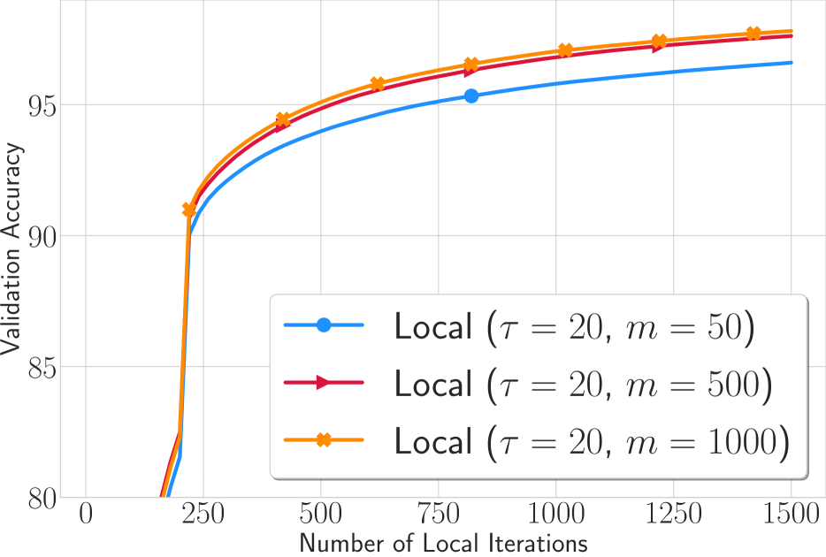
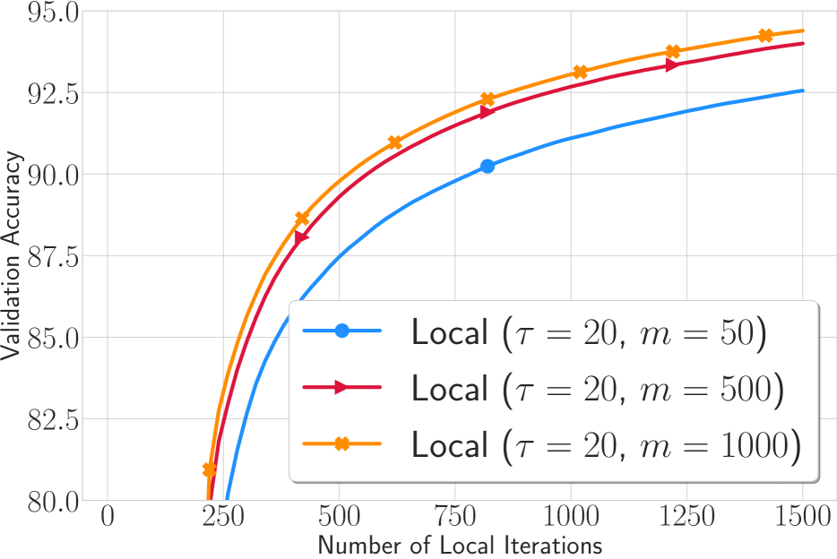
(a) Homogeneous Data Distribution

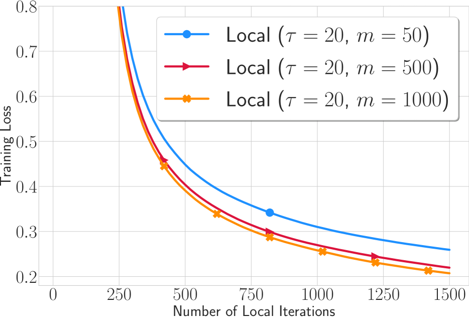
(b) Heterogeneous Data Distribution

Figure 1: Comparing the effect of model size using Local SGD on homogeneous and heterogeneous data distribution. By changing the model size from $m=50$ to $m=1000$, the model converges faster. In heterogeneous setting the increase in the model size has more impact on the convergence rate than the homogeneous setting.

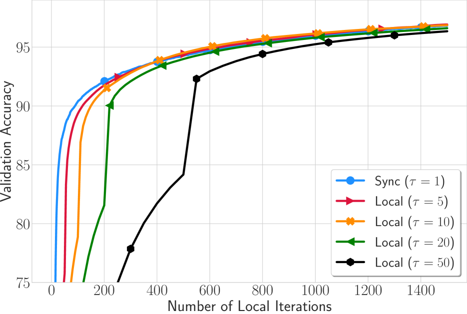
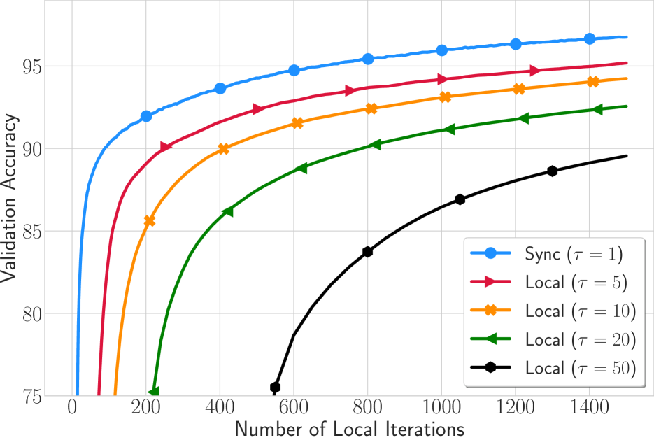
(a) Homogeneous Data Distribution

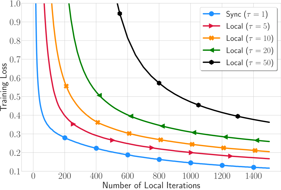
(b) Heterogeneous Data Distribution

Figure 2: Comparing the effect of synchronization gap (i.e., number of local updates $\tau$) on the model convergence. In this experiment the model size is fixed on $m=50$.

Effects of different synchronization gap $\tau$. Now, we fix the model size $m=50$ and change the synchronization gap $\tau$. We do the comparison between fully synchronous SGD and Local SGD with $\tau=5,10,20,50$. The results in Figure 2 shows that in both homogeneous and heterogeneous settings, the convergence rate becomes slower when synchronization gap increases. However, in the heterogeneous setting, increasing $\tau$ will decrease the convergence speed more significantly.

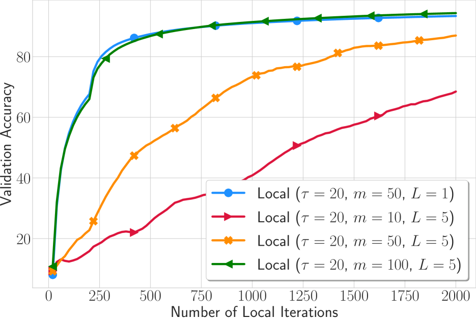
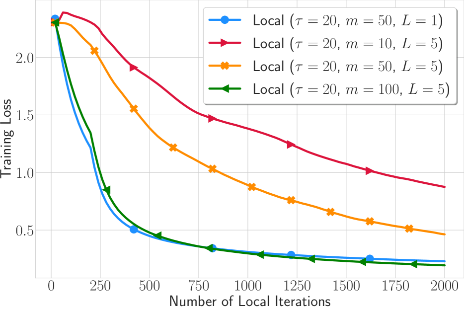
Figure 3: The effect of number of layer $L$. If we increase the number of layers to 5, compared to single layer, we need more neurons ($m$) to converge with the same rate as single layer.

Effects of number of layers $L$. When we increase the number of layers $L$, based on condition of $m$ in Theorem 2, we need to increase the number of neurons as well to achieve the same rate. For instance, Figure 3 shows the convergence rate of models with $L=5$ and various $m\in\{10,50,100\}$, compared with the single layer model with $m=50$. If we use the same number of neurons as the single layer (i.e. $m=10$ and $L=5$), it is evident that the model performs poorly. By increasing the number of neurons per layer, we can see that $m=100$ can make 5-layer model achieve the same performance of the single layer model, which has $10\times$ more neurons and more than $3\times$ bigger in terms of parameter size. This is consistent with Theorem 2, as increasing the number of layers requires significantly more neurons per layer compared to single layer counterpart to guarantees linear convergence rate.

7 Discussion and Future Works

In this paper, we proved that both Local GD and Local SGD that are originally proposed for communication efficient training of deep neural networks can achieve global minima of the training loss for over-parameterized deep ReLU networks. We make the first theoretical trial on the analysis of Local (S)GD on training Deep ReLU networks with multiple layers, but we do not claim that our results, e.g., number of required neurons and dependency on the number of layers, are optimal in any sense.

A number of future works/improvements are still exciting to explore:

Tightening the condition on the number of neurons. In the bounds obtained for both Local GD and SGD, the required number of neurons to has a heavy dependency on the number training samples $n$, which is worse than the single machine case. We are aware of some recent works [25, 24, 23] that demonstrate significantly reduced number of required neurons, and we believe incorporating their results can also improve our theory to entail tighter bounds.

Extension of analysis to other federated optimization methods. To further reduce the harm caused by multiple local updates, a line of recent studies proposed alternative methods to reduce the local model deviation [13, 30]. Establishing the convergence of these variants on deep non-smooth networks is another valuable research direction.

Extension to other neural network architectures. In this paper we only consider simple ReLU forward feed neural network, but as shown in the prior works [2, 36], single machine SGD can optimize more complicated neural network like CNN, ResNet or RNN as well. Hence, one natural future work is to extend our analysis on Local SGD to those neural network models.

Appendix A Proof of Theorem 1 (Local GD)

In this section we present the proof of convergence rate of Local GD (Theorem 1). Similar to analysis of Local SGD for smooth objectives [26, 14], we start from pertubed virtual iterates analysis. We let $\mathbf{W}(t)=\frac{1}{K}\sum_{i=1}^{K}\mathbf{W}^{(i)}(t)$ denote the virtual averaged iterates. Before providing the proof, let us first introduce some useful lemmas.

A.1 Proof of Technical Lemma

The following lemma is from Allen-Zhu et al’s seminal work [2], which characterizes the forward perturbation property of deep ReLU network:

Lemma 3 (Allen et al [2]).

Consider a weight matrices $\tilde{\mathbf{W}}$, $\mathbf{W}$ such that $\tilde{\mathbf{W}},\mathbf{W}\in\mathcal{B}(\mathbf{W}(0),\omega)$, with probability at least $1-\exp(-O(m\omega^{2/3}))$, the following facts hold:

$$\|f_{j,l-1}-f_{j,l-1}(0)\|\leq O\left(\omega L^{5/2}\sqrt{\log m}\right),$$

$$\|f_{j,l-1}\|\leq O(1),$$

$$\left\|\bm{v}^{\top}\mathbf{V}({\mathbf{D}}_{j,L}{\mathbf{W}}_{L}\cdots{\mathbf{D}}_{j,l+1}{\mathbf{W}}_{l+1}{\mathbf{D}}_{j,l}-\tilde{\mathbf{D}}_{j,L}\tilde{\mathbf{W}}_{L}\cdots\tilde{\mathbf{D}}_{j,l+1}\tilde{\mathbf{W}}_{l+1}\tilde{\mathbf{D}}_{j,l})\right\|\leq O\left(\omega^{1/3}L^{2}\sqrt{m\log m/d}\right)\cdot\|\bm{v}\|,$$

$$\|f_{j,l-1}-\tilde{f}_{j,l-1}\|\leq O\left(L^{3/2}\|\mathbf{W}-\tilde{\mathbf{W}}\|_{2}\right),$$

$$\left\|\bm{v}^{\top}\mathbf{V}({\mathbf{D}}_{j,L}{\mathbf{W}}_{L}\cdots{\mathbf{D}}_{j,l+1}{\mathbf{W}}_{l+1}{\mathbf{D}}_{j,l}\right\|\leq O\left(\sqrt{m/d}\right)\cdot\|\bm{v}\|,$$

where $\bm{v}$ is arbitrary vector, $f_{j,l-1}(0)=\sigma(\mathbf{W}_{l}(0)\sigma(\mathbf{W}_{l-1}(0)\cdots\sigma(\mathbf{W}_{1}(0)\bm{x}_{j})))$.

The following lemma establishes a bound on the deviation between local models and (virtual) averaged global model in terms of global loss.

Lemma 4.

For Local GD, let $t_{c}$ denote the latest communication stage of before iteration $t$. If the condition that $L_{i}(\mathbf{W}^{(i)}(t))\leq L_{i}(\mathbf{W}(t_{c}))$ for any $t_{c}\leq t\leq t_{c}+\tau-1$ holds, then the following statement holds true for $t_{c}\leq t\leq t_{c}+\tau-1$:

$$\left\|\mathbf{W}^{(i)}(t)-\mathbf{W}(t_{c})\right\|^{2}_{\mathrm{F}} \leq O\left((\eta^{2}\tau^{2}+\eta^{2}\tau)\frac{mn}{d}\right)L_{i}(\mathbf{W}(t_{c})).$$

where $K$ is the number of devices, $\tau$ is the number of local updates between two consecutive rounds of synchronization, $n$ is the size of each local data shard, and $m$ is the number of neurons in hidden layer.

Proof.

According to updating rule we have:

$$\left\|\mathbf{W}^{(i)}(t+1)-\mathbf{W}(t_{c})\right\|^{2}_{\mathrm{F}}= \left\|\mathbf{W}^{(i)}(t)-\eta\nabla L_{i}(\mathbf{W}^{(i)}(t))-\mathbf{W}(t_{c})\right\|^{2}_{\mathrm{F}}$$

$$=\left\|\mathbf{W}^{(i)}(t)-\mathbf{W}(t_{c})\right\|^{2}_{\mathrm{F}}-2\eta\left\langle\nabla L_{i}(\mathbf{W}^{(i)}(t)),\mathbf{W}^{(i)}(t)-\mathbf{W}(t_{c})\right\rangle$$

$$\quad+\eta^{2}\|\nabla L_{i}(\mathbf{W}^{(i)}(t))\|^{2}_{\mathrm{F}}$$

$$=\left\|\mathbf{W}^{(i)}(t)-\mathbf{W}(t_{c})\right\|^{2}_{\mathrm{F}}+2\eta\left\langle\nabla L_{i}(\mathbf{W}^{(i)}(t)),\eta\sum_{t^{\prime}=t_{c}}^{t-1}\nabla L_{i}(\mathbf{W}^{(i)}(t))\right\rangle$$

$$\quad+\eta^{2}\|\nabla L_{i}(\mathbf{W}^{(i)}(t))\|^{2}_{\mathrm{F}}$$

$$=\left\|\mathbf{W}^{(i)}(t)-\mathbf{W}(t_{c})\right\|^{2}_{\mathrm{F}}+2\eta^{2}\tau\left\langle\nabla L_{i}(\mathbf{W}^{(i)}(t)),\frac{1}{\tau}\sum_{t^{\prime}=t_{c}}^{t-1}\nabla L_{i}(\mathbf{W}^{(i)}(t))\right\rangle$$

$$\quad+\eta^{2}\|\nabla L_{i}(\mathbf{W}^{(i)}(t))\|^{2}_{\mathrm{F}}.$$

Applying the identity $\langle\bm{a},\bm{b}\rangle=\frac{1}{2}\|\bm{a}\|^{2}+\frac{1}{2}\|\bm{b}\|^{2}-\frac{1}{2}\|\bm{a}-\bm{b}\|^{2}$ on the cross term yields:

$$\left\|\mathbf{W}^{(i)}(t+1)-\mathbf{W}(t_{c})\right\|^{2}_{\mathrm{F}}$$

$$=\left\|\mathbf{W}^{(i)}(t)-\eta\nabla L_{i}(\mathbf{W}^{(i)}(t))-\mathbf{W}(t_{c})\right\|^{2}_{\mathrm{F}}$$

$$\leq\left\|\mathbf{W}^{(i)}(t)-\mathbf{W}(t_{c})\right\|^{2}_{\mathrm{F}}+\eta^{2}(t-t_{c})\left(\left\|\nabla L_{i}(\mathbf{W}^{(i)}(t))\right\|^{2}+\left\|\frac{1}{(t-t_{c})}\sum_{t^{\prime}=t_{c}}^{t-1}\nabla L_{i}(\mathbf{W}^{(i)}(t))\right\|^{2}\right)$$

$$\quad+\eta^{2}\|\nabla L_{i}(\mathbf{W}^{(i)}(t))\|^{2}_{\mathrm{F}}$$

$$\leq\left\|\mathbf{W}^{(i)}(t)-\mathbf{W}(t_{c})\right\|^{2}_{\mathrm{F}}+\eta^{2}(t-t_{c})\left(\left\|\nabla L_{i}(\mathbf{W}^{(i)}(t))\right\|^{2}+\frac{1}{t-t_{c}}\sum_{t^{\prime}=t_{c}}^{t-1}\left\|\nabla L_{i}(\mathbf{W}^{(i)}(t))\right\|^{2}\right)$$

$$\quad+\eta^{2}\|\nabla L_{i}(\mathbf{W}^{(i)}(t))\|^{2}_{\mathrm{F}}.$$

Plugging the gradient upper bound from Lemma 2 yields:

$$\left\|\mathbf{W}^{(i)}(t+1)-\mathbf{W}(t_{c})\right\|^{2}_{\mathrm{F}}$$

$$=\left\|\mathbf{W}^{(i)}(t)-\eta\nabla L_{i}(\mathbf{W}^{(i)}(t))-\mathbf{W}(t_{c})\right\|^{2}_{\mathrm{F}}$$

$$\leq\left\|\mathbf{W}^{(i)}(t)-\mathbf{W}(t_{c})\right\|^{2}_{\mathrm{F}}+\eta^{2}(t-t_{c})\left(O\big{(}\frac{mn}{d}\big{)}L_{i}(\mathbf{W}^{(i)}(t))+\frac{1}{t-t_{c}}\sum_{t^{\prime}=t_{c}}^{t-1}O\big{(}\frac{mn}{d}\big{)}L_{i}(\mathbf{W}^{(i)}(t^{\prime}))\right)$$

$$\quad+\eta^{2}O\big{(}\frac{mn}{d}\big{)}L_{i}(\mathbf{W}^{(i)}(t)).$$

Since we assume $L_{i}(\mathbf{W}^{(i)}(t))\leq L_{i}(\mathbf{W}(t_{c}))$ for any $t_{c}\leq t\leq t_{c}+\tau-1$, so we have:

$$\left\|\mathbf{W}^{(i)}(t+1)-\mathbf{W}(t_{c})\right\|^{2}_{\mathrm{F}} =\left\|\mathbf{W}^{(i)}(t)-\eta\nabla L_{i}(\mathbf{W}^{(i)}(t))-\mathbf{W}(t_{c})\right\|^{2}_{\mathrm{F}}$$

$$\leq\left\|\mathbf{W}^{(i)}(t)-\mathbf{W}(t_{c})\right\|^{2}_{\mathrm{F}}+\eta^{2}\tau\left(O\big{(}\frac{mn}{d}\big{)}L_{i}(\mathbf{W}^{(i)}(t_{c}))+O\big{(}\frac{mn}{d}\big{)}L_{i}(\mathbf{W}^{(i)}(t_{c}))\right)$$

$$\quad+\eta^{2}O\big{(}\frac{mn}{d}\big{)}L_{i}(\mathbf{W}^{(i)}(t_{c})).$$

Doing the telescoping sum from $t+1$ to $t_{c}$ will conclude the proof:

$$\left\|\mathbf{W}^{(i)}(t+1)-\mathbf{W}(t_{c})\right\|^{2}_{\mathrm{F}} \leq O\left((\eta^{2}\tau^{2}+\eta^{2}\tau)\frac{mn}{d}\right)L_{i}(\mathbf{W}^{(i)}(t_{c})).$$

∎

The next lemma is the key result in our proof, which characterizes the semi gradient Lipschitzness property of ReLU neural network.

Lemma 5 (Semi-gradient Lipschitzness).

For Local GD, at any iteration $t$, if $\mathbf{W},\tilde{\mathbf{W}}\in\mathcal{B}(\bm{W}(0),\omega)$, then with probability at least $1-\exp\left(-\Omega(m\omega^{2/3})\right)$, the following statement holds true:

$$\frac{1}{K}\sum_{i=1}^{K}\left\|\nabla_{\mathbf{W}}L_{i}(\mathbf{W})-\nabla_{\tilde{\mathbf{W}}}L_{i}(\tilde{\mathbf{W}})\right\|^{2}_{\mathrm{F}} \leq O\left(\frac{mL^{4}}{d}\left\|\mathbf{W}-\tilde{\mathbf{W}}\right\|_{2}^{2}\right)+O\left(\frac{\omega^{2/3}L^{5}{m\log m}}{d}+\frac{\omega^{2}L^{6}{m\log m}}{d}\right)L(\tilde{\mathbf{W}}),$$

where $K$ is the number of devices, $\tau$ is the number of local updates between two consecutive rounds of synchronization, $n$ is the size of each local data shard, and $m$ is the number of neurons in hidden layer.

Proof.

Observe that:

$$\frac{1}{K}\sum_{i=1}^{K}\left\|\nabla_{\mathbf{W}}L_{i}(\mathbf{W})-\nabla_{\tilde{\mathbf{W}}}L_{i}(\tilde{\mathbf{W}})\right\|^{2}_{\mathrm{F}}=\frac{1}{K}\sum_{i=1}^{K}\sum_{l=1}^{L}\left\|\nabla_{\mathbf{W}_{l}}L_{i}(\mathbf{W})-\nabla_{\tilde{\mathbf{W}}_{l}}L_{i}(\tilde{\mathbf{W}})\right\|^{2}_{\mathrm{F}}.$$

Let $f_{j}^{(i)}=\mathbf{V}\mathbf{D}^{(i)}_{j,L}\mathbf{W}^{(i)}_{L}\cdots\mathbf{D}_{j,1}\mathbf{W}^{(i)}_{1}\bm{x}_{j}$ and $\mathbf{L}^{(i)}_{j}=f_{j}^{(i)}-\bm{y}_{j}$. Now we examine the difference of the gradients:

$$\nabla_{\mathbf{W}_{l}}L_{i}(\mathbf{W})-\nabla_{\tilde{\mathbf{W}}_{l}}L_{i}(\tilde{\mathbf{W}})$$

$$=\frac{1}{n}\sum_{j=1}^{n}\left[(\mathbf{L}^{(i)}_{j}{}^{\top}\mathbf{V}\mathbf{D}_{j,L}\mathbf{W}_{L}\cdots\mathbf{D}_{j,l+1}\mathbf{W}_{l+1}\mathbf{D}_{j,l})^{\top}(f_{j,l-1}^{(i)}){}^{\top}-({\tilde{\mathbf{L}}^{(i)}_{j}}{}^{\top}\mathbf{V}\tilde{\mathbf{D}}_{j,L}\tilde{\mathbf{W}}_{L}\cdots\tilde{\mathbf{D}}_{j,l+1}\tilde{\mathbf{W}}_{l+1}\tilde{\mathbf{D}}_{j,l})^{\top}(\tilde{f}_{j,l-1}^{(i)})^{\top}\right]$$

$$=\frac{1}{n}\sum_{j=1}^{n}\left[(({\mathbf{L}^{(i)}_{j}}^{\top}-{\tilde{\mathbf{L}}^{(i)}_{j}}{}^{\top})\mathbf{V}\mathbf{D}_{j,L}\mathbf{W}_{L}\cdots\mathbf{D}_{j,l+1}\mathbf{W}_{l+1}\mathbf{D}_{j,l})^{\top}(f_{j,l-1}^{(i)}){}^{\top}\right]$$

$$\quad+\frac{1}{n}\sum_{j=1}^{n}\left[\left({\tilde{\mathbf{L}}^{(i)}_{j}}{}^{\top}\mathbf{V}({\mathbf{D}}_{j,L}{\mathbf{W}}_{L}\cdots{\mathbf{D}}_{j,l+1}{\mathbf{W}}_{l+1}{\mathbf{D}}_{j,l}-\tilde{\mathbf{D}}_{j,L}\tilde{\mathbf{W}}_{L}\cdots\tilde{\mathbf{D}}_{j,l+1}\tilde{\mathbf{W}}_{l+1}\tilde{\mathbf{D}}_{j,l})\right)^{\top}({f}_{j,l-1}^{(i)}){}^{\top}\right]$$

$$\quad+\frac{1}{n}\sum_{j=1}^{n}\left[({\tilde{\mathbf{L}}^{(i)}_{j}}{}^{\top}\mathbf{V}\tilde{\mathbf{D}}_{j,L}\tilde{\mathbf{W}}_{L}\cdots\tilde{\mathbf{D}}_{j,l+1}\tilde{\mathbf{W}}_{l+1}\tilde{\mathbf{D}}_{j,l})^{\top}({f}_{j,l-1}^{(i)}-\tilde{f}_{j,l-1}^{(i)}){}^{\top}\right].$$

According to Lemma 3 we know the following facts:

$$\|f_{j,l-1}^{(i)}-\tilde{f}_{j,l-1}^{(i)}\|\leq O\left(\omega L^{5/2}\sqrt{\log m}\right),$$

$$\|f_{j,l-1}^{(i)}\|\leq O(1),$$

$$\left\|\left(\tilde{\mathbf{L}}^{(i)}_{j}{}^{\top}\mathbf{V}({\mathbf{D}}_{j,L}{\mathbf{W}}_{L}\cdots{\mathbf{D}}_{j,l+1}{\mathbf{W}}_{l+1}{\mathbf{D}}_{j,l}-\tilde{\mathbf{D}}_{j,L}\tilde{\mathbf{W}}_{L}\cdots\tilde{\mathbf{D}}_{j,l+1}\tilde{\mathbf{W}}_{l+1}\tilde{\mathbf{D}}_{j,l})\right)^{\top}\right\|\leq O\left(\omega^{1/3}L^{2}\sqrt{m\log m/d}\right)\cdot\|\tilde{\mathbf{L}}^{(i)}_{j}\|,$$

$$\left\|\mathbf{L}^{(i)}_{j}{}^{\top}-\tilde{\mathbf{L}}^{(i)}_{j}{}^{\top}\right\|_{\mathrm{F}}=\left\|\mathbf{V}\sigma(\mathbf{W}_{L}\cdots\sigma(\mathbf{W}_{1}\bm{x}_{j}))-\mathbf{V}\sigma(\tilde{\mathbf{W}}_{L}\cdots\sigma(\tilde{\mathbf{W}}_{1}\bm{x}_{j}))\right\|\leq O\left(L^{3/2}\left\|\mathbf{W}-\tilde{\mathbf{W}}\right\|_{2}\right),$$

$$\left\|(\mathbf{L}^{(i)}_{j}{}^{\top}-\tilde{\mathbf{L}}^{(i)}_{j}{}^{\top})\mathbf{V}\mathbf{D}_{j,L}\mathbf{W}_{L}\cdots\mathbf{D}_{j,l+1}\mathbf{W}_{l+1}\mathbf{D}_{j,l})^{\top}\right\|\leq O\left(\sqrt{m/d}\cdot L^{3/2}\left\|\mathbf{W}-\tilde{\mathbf{W}}\right\|_{2}\right).$$

So we have the following bound for Frobenius norm:

$$\left\|\nabla_{\mathbf{W}_{l}}L_{i}(\mathbf{W})-\nabla_{\tilde{\mathbf{W}}_{l}}L_{i}(\tilde{\mathbf{W}})\right\|_{\mathrm{F}}^{2}$$

$$\leq\left(O\left(\sqrt{m/d}\cdot L^{3/2}\left\|\mathbf{W}-\tilde{\mathbf{W}}\right\|_{2}\right)+O\left(\omega^{1/3}L^{2}\sqrt{m\log m/d}\right)\cdot\|\tilde{\mathbf{L}}^{(i)}_{j}\|+O\left(\omega L^{5/2}\sqrt{m\log m/d}\right)\|\tilde{\mathbf{L}}^{(i)}_{j}\|\right)^{2}$$

$$\leq O\left({m/d}\cdot L^{3}\left\|\mathbf{W}-\tilde{\mathbf{W}}\right\|_{2}^{2}\right)+O\left(\omega^{2/3}L^{4}{m\log m/d}+\omega^{2}L^{5}{m\log m/d}\right)\|\tilde{\mathbf{L}}^{(i)}_{j}\|^{2}.$$

Hence we can conclude the proof:

$$\frac{1}{K}\sum_{i=1}^{K}\left\|\nabla_{\mathbf{W}}L_{i}(\mathbf{W})-\nabla_{\tilde{\mathbf{W}}}L_{i}(\tilde{\mathbf{W}})\right\|^{2}_{\mathrm{F}}=\frac{1}{K}\sum_{i=1}^{K}\sum_{l=1}^{L}\left\|\nabla_{\mathbf{W}_{l}}L_{i}(\mathbf{W})-\nabla_{\tilde{\mathbf{W}}_{l}}L_{i}(\tilde{\mathbf{W}})\right\|^{2}_{\mathrm{F}}$$

$$\leq O\left(\frac{mL^{4}}{d}\left\|\mathbf{W}-\tilde{\mathbf{W}}\right\|_{2}^{2}\right)+O\left(\frac{\omega^{2/3}L^{5}{m\log m}}{d}+\frac{\omega^{2}L^{6}{m\log m}}{d}\right)L(\tilde{\mathbf{W}}).$$

∎

Lemma 6.

For Local GD, at any iteration $t$ in between two communication rounds: $t_{c}\leq t\leq t_{c}+\tau-1$ and $i\in[K]$, if $\mathbf{W}^{(i)}(t)\in\mathcal{B}(\bm{W}(0),\omega)$, then with probability at least $1-\exp\left(-\Omega(m\omega^{2/3})\right)$, the following statement holds true:

$$L_{i}(\mathbf{W}^{(i)}(t))\leq L_{i}(\mathbf{W}^{(i)}(t-1))\leq\cdots\leq L_{i}(\mathbf{W}^{(i)}(t_{c})).$$

Proof.

According to updating rule and the semi smoothness property:

$$L_{i}(\mathbf{W}^{(i)}(t))\leq L_{i}(\mathbf{W}^{(i)}(t-1))+\left[\left\langle\nabla L_{i}(\mathbf{W}^{(i)}(t-1)),\mathbf{W}^{(i)}(t)-\mathbf{W}^{(i)}(t-1)\right\rangle\right]$$

$$\quad+C^{\prime}\sqrt{L_{i}(\mathbf{W}^{(i)}(t))}\cdot\frac{\omega^{1/3}L^{2}\sqrt{m\log(m)}}{\sqrt{d}}\cdot\|\mathbf{W}^{(i)}(t)-\mathbf{W}^{(i)}(t-1)\|_{2}+\frac{C^{\prime\prime}L^{2}m}{d}\|\mathbf{W}^{(i)}(t)-\mathbf{W}^{(i)}(t-1)\|^{2}_{2}$$

$$\leq L(\mathbf{W}^{(i)}(t-1))-\eta\left\langle\nabla L(\mathbf{W}^{(i)}(t-1)),\nabla L_{i}(\mathbf{W}^{(i)}(t-1))\right\rangle$$

$$\quad+\eta C^{\prime}\sqrt{L_{i}(\mathbf{W}^{(i)}(t-1))}\cdot\frac{\omega^{1/3}L^{2}\sqrt{m\log(m)}}{\sqrt{d}}\cdot\left\|\nabla L_{i}(\mathbf{W}^{(i)}(t-1))\right\|_{2}+\eta^{2}\frac{C^{\prime\prime}L^{2}m}{d}\mathbb{E}\left\|\nabla L_{i}(\mathbf{W}^{(i)}(t-1))\right\|^{2}_{2}$$

$$\stackrel{{\scriptstyle\text{\char 192}}}{{\leq}}\left(1-\Omega\left({\frac{\eta\tau m\phi}{dn^{2}}}\right)\right)L_{i}(\mathbf{W}^{(i)}(t-1)),$$

where in ➀ we plug in the gradient upper bound from Lemma 2. According to our choice of $\eta$, we can conclude that

$$L_{i}(\mathbf{W}^{(i)}(t))\leq L_{i}(\mathbf{W}^{(i)}(t-1))\leq\cdots\leq L_{i}(\mathbf{W}^{(i)}(t_{c})).$$

∎

A.2 Proof of Theorem 1

With the key lemmas in place, we now prove Theorem 1 by induction. Assume the following induction hypotheses hold for $h\leq t$:

$$\textbf{(I)}\quad\left\|\mathbf{W}(h)-\mathbf{W}(0)\right\|\leq\omega,\left\|\mathbf{W}^{(i)}(h)-\mathbf{W}(0)\right\|\leq\omega,\quad\forall i\in[K],$$

$$\textbf{(II)}\quad L(\mathbf{W}(t_{c}))\leq\left(1-\Omega\left(\frac{\eta\tau m\phi}{dn^{2}}\right)\right)^{c}L(\mathbf{W}(0))$$

where $\omega=O\big{(}\phi^{3/2}n^{-6}L^{-6}\log^{-3/2}(m)\big{)}$, and $t_{c}$ is the latest communication round of $h$, which is also $c$th communication round. Then we shall show the above two statements hold for $t+1$.

A.2.1 Proof of inductive hypothesis I

Step 1: Bounded virtual average iterates.

First we prove the first hypothesis for $t+1$: $\left\|\mathbf{W}(t+1)-\mathbf{W}(0)\right\|\leq\omega$. By the updating rule we know that:

$$\left\|\mathbf{W}(t+1)-\mathbf{W}(0)\right\| \leq\eta\sum_{j=1}^{t}\left\|\frac{1}{K}\sum_{i=1}^{K}\nabla L_{i}(\mathbf{W}^{(i)}(j))\right\|$$

$$\stackrel{{\scriptstyle\text{\char 192}}}{{\leq}}\eta\sum_{j=1}^{t}\frac{1}{K}\sum_{i=1}^{K}O(\sqrt{\frac{m}{d}})\sqrt{L_{i}(\mathbf{W}(j))}$$

$$\stackrel{{\scriptstyle\text{\char 193}}}{{\leq}}\eta\tau\sum_{j=1}^{c}\frac{1}{K}\sum_{i=1}^{K}O(\sqrt{\frac{m}{d}})\sqrt{L_{i}(\mathbf{W}(t_{c}))}$$

$$\leq\eta\tau\sum_{j=1}^{c}O(\sqrt{\frac{m}{d}})\sqrt{L(\mathbf{W}(t_{c}))},$$

where we apply the gradient upper bound (Lemma 2) in ➀ and the decreasing nature of local loss (Lemma 6) in ➁. Now we plug in induction hypothesis II to bound $L(\mathbf{W}(t_{c}))$:

$$\left\|\mathbf{W}(t+1)-\mathbf{W}(0)\right\| \leq\eta\tau\sum_{j=1}^{c}O(\sqrt{\frac{m}{d}})\sqrt{\left(1-\Omega\left(\frac{\eta\tau m\phi}{dn^{2}}\right)\right)^{c}L(\mathbf{W}(0))}$$

$$\leq\eta\tau O(\sqrt{\frac{m}{d}})\sum_{j=1}^{c}\left(1-\Omega\left(\frac{\eta\tau m\phi}{2dn^{2}}\right)\right)^{c}\sqrt{L(\mathbf{W}(0))}$$

$$\leq\eta\tau O(\sqrt{\frac{m}{d}})O\left(\frac{2dn^{2}}{\eta\tau m\phi}\right)\sqrt{L(\mathbf{W}(0))}$$

$$=O\left(\frac{2\sqrt{d}n^{2}}{\sqrt{m}\phi}\right)\sqrt{L(\mathbf{W}(0))}.$$

Since we choose $m\geq\frac{dn^{16}L^{12}\log^{3}m}{\phi^{5}}$, it follows that $\left\|\mathbf{W}(t+1)-\mathbf{W}(0)\right\|\leq\omega$.

Step 2: Bounded local iterates.

Then we prove the second hypothesis for $t+1$: $\left\|\mathbf{W}^{(i)}(t+1)-\mathbf{W}(0)\right\|\leq\omega$. By the updating rule we know that:

$$\left\|\mathbf{W}^{(i)}(t+1)-\mathbf{W}(0)\right\| \leq\eta\sum_{j=1}^{t}\left\|\nabla L_{i}(\mathbf{W}^{(i)}(j))\right\|$$

$$\leq\eta\sum_{j=1}^{t}O\left(\sqrt{\frac{m}{d}}\right)\sqrt{L_{i}(\mathbf{W}(j))}$$

$$\leq\eta\tau\sum_{j=1}^{c}O\left(\sqrt{\frac{m}{d}}\right)\sqrt{L_{i}(\mathbf{W}(t_{c}))}$$

$$\leq\eta\tau\sum_{j=1}^{c}O\left(\sqrt{\frac{m}{d}}\right)\sqrt{KL_{i}(\mathbf{W}(t_{c}))},$$

where we apply the gradient upper bound (Lemma 2) and the decreasing nature of local loss (Lemma 6). Now we plug in induction hypothesis II to bound $L(\mathbf{W}(t_{c}))$:

$$\left\|\mathbf{W}(t+1)-\mathbf{W}(0)\right\| \leq\eta\tau\sum_{j=1}^{c}O\left(\sqrt{\frac{m}{d}}\right)\sqrt{\left(1-\Omega\left(\frac{\eta\tau m\phi}{dn^{2}}\right)\right)^{c}L_{i}(\mathbf{W}(0))}$$

$$\leq\eta\tau O\left(\sqrt{K\frac{m}{d}}\right)\sum_{j=1}^{c}\left(1-\Omega\left(\frac{\eta\tau m\phi}{2dn^{2}}\right)\right)^{c}\sqrt{L_{i}(\mathbf{W}(0))}$$

$$\leq\eta\tau O\left(\sqrt{K\frac{m}{d}}\right)O\left(\frac{2dn^{2}}{\eta\tau m\phi}\right)\sqrt{L_{i}(\mathbf{W}(0))}$$

$$=O\left(\frac{2\sqrt{d}n^{2}}{\sqrt{m}\phi}\right)\sqrt{KL_{i}(\mathbf{W}(0))}.$$

Since we choose $m\geq\frac{Kdn^{12}L^{12}\log^{3}m}{\phi^{5}}$, it immediately follows that $\left\|\mathbf{W}^{(i)}(t+1)-\mathbf{W}(0)\right\|\leq\omega$ as desired.

A.2.2 Proof of inductive hypothesis II

Step 1: One iteration analysis from Semi-smoothness.

Now we proceed to prove that hypothesis II holds for $t+1$. If $t_{c}\leq t+1<t_{c+1}$, then the statement apparently holds for $t_{c}$. If $t+1\geq t_{c+1}$, we have to examine the upper bound for $L(\mathbf{W}(t_{c+1}))$. The first step is to characterize how global loss changes in one iteration. We use the technique from standard smooth non-convex optimization, but notice that here we only have semi-smooth objective. According to semi-smoothness (Lemma 1) and updating rule:

$$L(\mathbf{W}(t_{c+1}))\leq L(\mathbf{W}(t_{c}))+\left\langle\nabla L(\mathbf{W}(t_{c})),\mathbf{W}(t_{c+1})-\mathbf{W}(t_{c})\right\rangle$$

$$\quad+C^{\prime}\sqrt{L(\mathbf{W}(t_{c}))}\cdot\frac{\omega^{1/3}L^{2}\sqrt{m\log(m)}}{\sqrt{d}}\cdot\|\mathbf{W}(t_{c+1})-\mathbf{W}(t_{c})\|_{2}+\frac{C^{\prime\prime}L^{2}m}{d}\|\mathbf{W}(t_{c})-\mathbf{W}(t_{c})\|^{2}_{2}$$

$$\leq L(\mathbf{W}(t_{c}))-\left\langle\nabla L(\mathbf{W}(t_{c})),\eta\tau\frac{1}{\tau K}\sum_{i=1}^{K}\sum_{t^{\prime}=t_{c}}^{t_{c+1}-1}\nabla L_{i}(\mathbf{W}^{(i)}(t^{\prime}))\right\rangle$$

$$\quad+\eta\tau C^{\prime}\sqrt{L(\mathbf{W}(t_{c-1}))}\cdot\frac{\omega^{1/3}L^{2}\sqrt{m\log(m)}}{\sqrt{d}}\cdot\left\|\frac{1}{\tau K}\sum_{i=1}^{K}\sum_{t^{\prime}=t_{c}}^{t_{c+1}-1}\nabla L_{i}(\mathbf{W}^{(i)}(t^{\prime}))\right\|$$

$$\quad+\eta^{2}\frac{C^{\prime\prime}L^{2}m}{d}\left\|\frac{1}{K}\sum_{i=1}^{K}\sum_{t^{\prime}=t_{c}}^{t_{c+1}-1}\nabla L_{i}(\mathbf{W}^{(i)}(t^{\prime}))\right\|^{2}$$

$$\stackrel{{\scriptstyle\text{\char 192}}}{{\leq}}L(\mathbf{W}(t_{c}))-\frac{\eta\tau}{2}\left\|\nabla L(\mathbf{W}(t_{c}))\right\|^{2}_{\mathrm{F}}-\frac{\eta\tau}{2}\left\|\frac{1}{\tau K}\sum_{i=1}^{K}\sum_{t^{\prime}=t_{c}}^{t_{c+1}-1}\nabla L_{i}(\mathbf{W}^{(i)}(t))\right\|^{2}_{\mathrm{F}}$$

$$\quad+\frac{\eta\tau}{2}\left\|\nabla L(\mathbf{W}(t_{c}))-\frac{1}{\tau K}\sum_{i=1}^{K}\sum_{t^{\prime}=t_{c}}^{t_{c+1}-1}\nabla L_{i}(\mathbf{W}^{(i)}(t^{\prime}))\right\|^{2}_{\mathrm{F}}$$

$$\quad+\eta\tau C^{\prime}\sqrt{L(\mathbf{W}(t_{c}))}\cdot\frac{\omega^{1/3}L^{2}\sqrt{m\log(m)}}{2\sqrt{d}}$$

$$\quad\times\left(\left\|\nabla L(\mathbf{W}(t_{c}))\right\|_{\mathrm{F}}+\left\|\frac{1}{\tau K}\sum_{i=1}^{K}\sum_{t^{\prime}=t_{c}}^{t_{c+1}-1}\nabla L_{i}(\mathbf{W}^{(i)}(t^{\prime}))-\nabla L(\mathbf{W}(t_{c}))\right\|_{\mathrm{F}}\right)$$

$$\quad+\eta^{2}\frac{C^{\prime\prime}L^{2}m}{d}\left\|\frac{1}{K}\sum_{i=1}^{K}\sum_{t^{\prime}=t_{c}}^{t_{c+1}-1}\nabla L_{i}(\mathbf{W}^{(i)}(t^{\prime}))\right\|^{2}_{\mathrm{F}}$$

$$\leq L(\mathbf{W}(t_{c}))-\frac{\eta\tau}{2}\left\|\nabla L(\mathbf{W}(t_{c}))\right\|^{2}_{\mathrm{F}}-\left(\frac{\eta}{2\tau}-\frac{\eta^{2}C^{\prime\prime}L^{2}m}{d}\right)\left\|\frac{1}{K}\sum_{i=1}^{K}\sum_{t^{\prime}=t_{c}}^{t_{c+1}-1}\nabla L_{i}(\mathbf{W}^{(i)}(t^{\prime}))\right\|^{2}_{\mathrm{F}}$$

$$\quad+\frac{\eta}{2}\frac{1}{K}\sum_{i=1}^{K}\sum_{t^{\prime}=t_{c}}^{t_{c+1}-1}\left\|\nabla L_{i}(\mathbf{W}(t_{c}))-\nabla L_{i}(\mathbf{W}^{(i)}(t^{\prime}))\right\|^{2}_{\mathrm{F}}+\eta C^{\prime}\sqrt{L(\mathbf{W}(t))}\cdot\frac{\omega^{1/3}L^{2}\sqrt{m\log(m)}}{2\sqrt{d}}\left\|\nabla L(\mathbf{W}(t_{c}))\right\|_{\mathrm{F}}$$

$$\quad+\eta\tau C^{\prime}\cdot\frac{\omega^{1/3}L^{2}\sqrt{m\log(m)}}{2\sqrt{d}}\left(\left\|\nabla L(\mathbf{W}(t_{c}))-\frac{1}{\tau K}\sum_{i=1}^{K}\sum_{t^{\prime}=t_{c}}^{t_{c+1}-1}\nabla L_{i}(\mathbf{W}^{(i)}(t^{\prime}))\right\|_{\mathrm{F}}\sqrt{L(\mathbf{W}(t_{c}))}\right),$$

where in ➀ we use the identity $\langle\bm{a},\bm{b}\rangle=\frac{1}{2}\|\bm{a}\|^{2}+\frac{1}{2}\|\bm{b}\|^{2}-\frac{1}{2}\|\bm{a}-\bm{b}\|^{2}$. We plug in the semi gradient Lipschitzness from Lemma 5 and gradient bound from Lemma 2 in last inequality, and use the fact that $\frac{\eta}{2\tau}-\frac{\eta^{2}C^{\prime\prime}L^{2}m}{d}\geq 0$ to get:

$$L(\mathbf{W}(t_{c+1})) \leq L(\mathbf{W}(t_{c}))-\Omega\left(\frac{\eta\tau m\phi}{dn^{2}}\right)L(\mathbf{W}_{t_{c}})$$

$$\quad+\frac{\eta\tau}{2}\left(O\left(\frac{mL^{4}}{d}\left\|\mathbf{W}^{(i)}(t^{\prime})-\mathbf{W}(t_{c})\right\|_{2}^{2}\right)+O\left(\frac{\omega^{2/3}L^{5}{m\log m}}{d}+\frac{\omega^{2}L^{6}{m\log m}}{d}\right)L(\mathbf{W}(t_{c}))\right)$$

$$\quad+\eta\tau C^{\prime}\cdot\frac{\omega^{1/3}L^{2}{m\log(m)}}{2{d}}L(\mathbf{W}({t_{c}}))$$

$$\quad+\eta\tau C^{\prime}\cdot\frac{\omega^{1/3}L^{2}\sqrt{m\log(m)}}{2\sqrt{d}}$$

$$\quad\times\left(\sqrt{O\left(\frac{mL^{4}}{d}\left\|\mathbf{W}^{(i)}(t^{\prime})-\mathbf{W}(t_{c})\right\|_{2}^{2}\right)+O\left(\frac{\omega^{2/3}L^{5}{m\log m}}{d}+\frac{\omega^{2}L^{6}{m\log m}}{d}\right)L(\mathbf{W}(t_{c}))}L(\mathbf{W}(t_{c})\right),$$

Choosing $\omega=\frac{\phi^{3/2}}{C_{\omega}n^{6}L^{6}\log(m)^{3/2}}$ where $C_{\omega}$ is some large constant and plugging in local model deviation bound from Lemma 4, to get the main recursion relation as follows:

$$L(\mathbf{W}(t_{c+1})) \leq\left(1-\Omega\left(\frac{\eta\tau m\phi}{dn^{2}}\right)\right)L(\mathbf{W}(t_{c})).$$ (4)

Unrolling the recursion and plugging in $\eta=O(\frac{dn^{2}}{\tau m\phi})$ will conclude the proof:

$$L(\mathbf{W}(T))\leq\exp(-R)L(\mathbf{W}(0))=\epsilon$$

$$\Longleftrightarrow R=O\left(\log\frac{1}{\epsilon}\right).$$

Appendix B Proof of Theorem 2 (Local SGD)

In this section we will present the proof of convergence rate of Local SGD (Theorem 2). Before that, let us first introduce some useful lemmas.

B.1 Proof of Technical Lemma

The following lemma establishes the boundedness of the stochastic gradient.

Lemma 7 (Bounded stochastic gradient).

For Local SGD, the following statement holds true for stochastic gradient at any iteration $t$:

$$\mathbb{E}_{S_{t}}\left[\left\|\frac{1}{K}\sum_{i=1}^{K}\mathbf{G}_{i}^{(t)}\right\|^{2}\right]\leq O\left(\frac{mL(\mathbf{W}(t_{c}))}{dK}\right),\left\|\frac{1}{K}\sum_{i=1}^{K}\mathbf{G}_{i}^{(t)}\right\|^{2}\leq O\left(\frac{mnL(\mathbf{W}(t_{c}))}{d}\right),$$

where $S_{t}=\{(\tilde{\bm{x}}_{i},\tilde{y}_{i})\}_{i=1}^{K}$ are the set of randomly sampled data to compute $\frac{1}{K}\sum_{i=1}^{K}\mathbf{G}_{i}^{(t)}$, $K$ is the number of devices, $\tau$ is the number of local updates between two consecutive rounds of synchronization, $n$ is the size of each local data shard, $d$ is the dimension of input data, and $m$ is the number of neurons in hidden layer.

Proof.

Observe the following facts:

$$\mathbb{E}_{S_{t}}\left[\left\|\frac{1}{K}\sum_{i=1}^{K}\mathbf{G}_{i}^{(t)}\right\|^{2}\right] =\frac{1}{K^{2}}\sum_{i=1}^{K}\mathbb{E}\left[\left\|\nabla\ell(\mathbf{W}^{(i)}(t);\tilde{\bm{x}}_{i},\tilde{y}_{i})\right\|^{2}\right]$$

$$=\frac{1}{K^{2}}\sum_{i=1}^{K}\frac{1}{n}\sum_{(\bm{x}_{j},y_{j})\in S_{i}}\left\|\nabla\ell(\mathbf{W}^{(i)}(t);\bm{x}_{j},y_{j})\right\|^{2}$$

$$\leq\frac{1}{K^{2}}\sum_{i=1}^{K}O(m/d)L_{i}(\mathbf{W}^{(i)}(t)),$$

where we plug in the gradiet upper bound from Lemma 2. According to the shrinkage of local loss (Lemma 9), we can conclude that:

$$\mathbb{E}_{S_{t}}\left[\left\|\frac{1}{K}\sum_{i=1}^{K}\mathbf{G}_{i}^{(t)}\right\|^{2}\right]\leq O\left(\frac{mL(\mathbf{W}(t_{c}))}{dK}\right).$$

Now we switch to prove the second statement by observing that:

$$\left\|\frac{1}{K}\sum_{i=1}^{K}\mathbf{G}_{i}^{(t)}\right\|^{2} =\frac{1}{K}\sum_{i=1}^{K}\left\|\nabla\ell(\mathbf{W}^{(i)}(t);\tilde{\bm{x}}_{i},\tilde{y}_{i})\right\|^{2}$$

$$\leq\frac{1}{K}\sum_{i=1}^{K}O(mn/d)L_{i}(\mathbf{W}^{(i)}(t))$$

$$\leq\frac{1}{K}\sum_{i=1}^{K}O(mn/d)L_{i}(\mathbf{W}^{(i)}(t_{c})),$$

which completes the proof. ∎

The next lemma is similar to Lemma 4, but it characterizes the local model deviation under stochastic setting. Hence, it will be inevitably looser than the deterministic version (Lemma 4).

Lemma 8.

For Local SGD, let $t_{c}$ denote the latest communication stage of before iteration $t$. If the condition that $L_{i}(\mathbf{W}^{(i)}(t))\leq L_{i}(\mathbf{W}(t_{c}))$ for any $t_{c}\leq t\leq t_{c}+\tau-1$ holds, then the following statement holds true for $t_{c}\leq t\leq t_{c}+\tau-1$:

$$\left\|\mathbf{W}^{(i)}(t)-\mathbf{W}(t_{c})\right\|^{2}_{\mathrm{F}} \leq O\left((\eta^{2}\tau^{2}+\eta^{2}\tau)\frac{mn}{d}\right)L_{i}(\mathbf{W}(t_{c})),$$

where $K$ is the number of devices, $\tau$ is the number of local updates between two consecutive rounds of synchronization, $n$ is the size of each local data shard, and $m$ is the number of neurons in hidden layer.

Proof.

According to updating rule:

$$\mathbb{E}\left\|\mathbf{W}^{(i)}(t+1)-\mathbf{W}(t_{c})\right\|^{2}_{\mathrm{F}} =\mathbb{E}\left\|\mathbf{W}^{(i)}(t)-\eta\mathbf{G}^{(t)}_{i}-\mathbf{W}(t_{c})\right\|^{2}_{\mathrm{F}}$$

$$=\mathbb{E}\left\|\mathbf{W}^{(i)}(t)-\mathbf{W}(t_{c})\right\|^{2}_{\mathrm{F}}-2\eta\mathbb{E}\left\langle\nabla L_{i}(\mathbf{W}^{(i)}(t)),\mathbf{W}^{(i)}(t)-\mathbf{W}(t_{c})\right\rangle$$

$$\quad+\eta^{2}\mathbb{E}\|\mathbf{G}^{(t)}_{i}\|^{2}_{\mathrm{F}}$$

$$=\mathbb{E}\left\|\mathbf{W}^{(i)}(t)-\mathbf{W}(t_{c})\right\|^{2}_{\mathrm{F}}+2\eta\left\langle\nabla L_{i}(\mathbf{W}^{(i)}(t)),\eta\sum_{t^{\prime}=t_{c}}^{t-1}\nabla L_{i}(\mathbf{W}^{(i)}(t))\right\rangle$$

$$\quad+\eta^{2}\mathbb{E}\|\mathbf{G}^{(t)}_{i}\|^{2}_{\mathrm{F}}$$

$$=\mathbb{E}\left\|\mathbf{W}^{(i)}(t)-\mathbf{W}(t_{c})\right\|^{2}_{\mathrm{F}}+2\eta^{2}(t-t_{c})\left\langle\nabla L_{i}(\mathbf{W}^{(i)}(t)),\frac{1}{(t-t_{c})}\sum_{t^{\prime}=t_{c}}^{t-1}\nabla L_{i}(\mathbf{W}^{(i)}(t))\right\rangle$$

$$\quad+\eta^{2}\mathbb{E}\|\mathbf{G}^{(t)}_{i}\|^{2}_{\mathrm{F}}.$$

Applying the identity $\langle\bm{a},\bm{b}\rangle=\frac{1}{2}\|\bm{a}\|^{2}+\frac{1}{2}\|\bm{b}\|^{2}-\frac{1}{2}\|\bm{a}-\bm{b}\|^{2}$ on the cross term we have:

$$\mathbb{E}\left\|\mathbf{W}^{(i)}(t+1)-\mathbf{W}(t_{c})\right\|^{2}_{\mathrm{F}} \leq\mathbb{E}\left\|\mathbf{W}^{(i)}(t)-\mathbf{W}(t_{c})\right\|^{2}_{\mathrm{F}}$$

$$\quad+\eta^{2}(t-t_{c})\left(\mathbb{E}\left\|\nabla L_{i}(\mathbf{W}^{(i)}(t))\right\|^{2}+\left\|\frac{1}{(t-t_{c})}\sum_{t^{\prime}=t_{c}}^{t-1}\nabla L_{i}(\mathbf{W}^{(i)}(t))\right\|^{2}\right)$$

$$\quad+\eta^{2}\frac{1}{n}\sum_{(\bm{x}_{j},y_{j})\in S_{i}}\left\|\nabla\ell(\mathbf{W}^{(i)}(t);\bm{x}_{j},y_{j})\right\|^{2}.$$

Plugging the gradient upper bound from Lemma 2 yields:

$$\mathbb{E}\left\|\mathbf{W}^{(i)}(t+1)-\mathbf{W}(t_{c})\right\|^{2}_{\mathrm{F}} \leq\mathbb{E}\left\|\mathbf{W}^{(i)}(t)-\mathbf{W}(t_{c})\right\|^{2}_{\mathrm{F}}$$

$$\quad+\eta^{2}(t-t_{c})\left(O\left(\frac{m}{d}\right)L_{i}(\mathbf{W}^{(i)}(t))+\frac{1}{t-t_{c}}\sum_{t^{\prime}=t_{c}}^{t-1}O\left(\frac{m}{d}\right)L_{i}(\mathbf{W}^{(i)}(t^{\prime}))\right)$$

$$\quad+\eta^{2}O\left(\frac{m}{d}\right)L_{i}(\mathbf{W}^{(i)}(t)).$$

Since we assume $L_{i}(\mathbf{W}^{(i)}(t))\leq L_{i}(\mathbf{W}(t_{c}))$ for any $t_{c}\leq t\leq t_{c}+\tau-1$, we have:

$$\mathbb{E}\left\|\mathbf{W}^{(i)}(t+1)-\mathbf{W}(t_{c})\right\|^{2}_{\mathrm{F}} \leq\mathbb{E}\left\|\mathbf{W}^{(i)}(t)-\mathbf{W}(t_{c})\right\|^{2}_{\mathrm{F}}+\eta^{2}\tau\left(O\big{(}\frac{m}{d}\big{)}L_{i}(\mathbf{W}^{(i)}(t_{c}))+O\big{(}\frac{m}{d}\big{)}L_{i}(\mathbf{W}^{(i)}(t_{c}))\right)$$

$$\quad+\eta^{2}O\big{(}\frac{m}{d}\big{)}L_{i}(\mathbf{W}(t_{c})).$$

Do the telescoping sum from $t+1$ to $t_{c}$ will conclude the proof:

$$\mathbb{E}\left\|\mathbf{W}^{(i)}(t+1)-\mathbf{W}(t_{c})\right\|^{2}_{\mathrm{F}} \leq O\left((\eta^{2}\tau^{2}+\eta^{2}\tau)\frac{m}{d}\right)L_{i}(\mathbf{W}(t_{c})).$$

∎

The next lemma will reveal the boundedness of objective in stochastic setting. The slight difference to the dynamic of objective in deterministic setting (Lemma 6) is that, we show the objective is strictly decreasing in Local GD, but here we only derive a small upper bound of it: $L_{i}(\mathbf{W}^{(i)}(t))\leq O(1)\cdot L_{i}(\mathbf{W}(t_{c}))$, with high probability. Even though it is not a strictly decreasing loss, it is enough to enable us to prove linear convergence of objective.

Lemma 9.

For Local SGD, at any iteration $t$ in between two communication rounds: $t_{c}\leq t\leq t_{c}+\tau-1$ and $i\in[K]$, if $\mathbf{W}^{(i)}(t)\in\mathcal{B}(\bm{W}(0),\omega)$, then with probability at least $1-\exp\left(-\Omega(m\omega^{2/3})\right)$, the following statement holds true:

$$L_{i}(\mathbf{W}^{(i)}(t))\leq O(1)\cdot L_{i}(\mathbf{W}(t_{c})).$$

Proof.

We examine the absolute value bound for $L_{i}(\mathbf{W}^{(i)}(t-1))$:

$$L_{i}(\mathbf{W}^{(i)}(t)) \leq L_{i}(\mathbf{W}^{(i)}(t-1))+\eta\left\|\nabla L_{i}(\mathbf{W}(t-1))\right\|\left\|\mathbf{G}^{(i)}(t)\right\|$$

$$\quad+\eta C^{\prime}\sqrt{L_{i}(\mathbf{W}^{(i)}(t-1))}\cdot\frac{\omega^{1/3}L^{2}\sqrt{m\log(m)}}{\sqrt{d}}\cdot\left\|\mathbf{G}^{(i)}(t)\right\|_{2}+\eta^{2}\frac{C^{\prime\prime}L^{2}m}{d}\left\|\mathbf{G}^{(i)}(t)\right\|^{2}_{2}$$

$$\leq L_{i}(\mathbf{W}^{(i)}(t-1))+\frac{\eta m\sqrt{n}}{d}L_{i}(\mathbf{W}^{(i)}(t-1))$$

$$\quad+\eta C^{\prime}\frac{\omega^{1/3}L^{2}m\sqrt{mn\log(m)}}{d\sqrt{d}}L_{i}(\mathbf{W}^{(i)}(t-1))+\eta^{2}\frac{C^{\prime\prime}L^{2}m^{2}n}{d^{2}}L_{i}(\mathbf{W}(t-1))$$

$$\leq\left(1+O\left(\frac{\eta m\sqrt{n}}{d}\right)\right)L_{i}(\mathbf{W}^{(i)}(t-1))$$

$$\leq\left(1+O\left(\frac{\phi}{m\tau n^{2.5}\log^{2}m}\right)\right)^{\tau}L_{i}(\mathbf{W}(t_{c}))$$

$$\leq\exp\left(\frac{\phi}{mn^{2.5}\log^{2}m}\right)L_{i}(\mathbf{W}(t_{c}))\leq O(1)\cdot L_{i}(\mathbf{W}(t_{c})).$$

∎

B.2 Proof of Theorem 2

With the above lemmas in hand, we can finally proceed to the proof of Theorem 2. We prove Theorem 2 by induction. Assume the following induction hypotheses hold for all $h\leq t$, with probability at least $1-e^{-\Omega((\log m)^{2})}$:

$$\textbf{(I)}\quad\left\|\mathbf{W}(h)-\mathbf{W}(0)\right\|\leq\omega,\left\|\mathbf{W}^{(i)}(h)-\mathbf{W}(0)\right\|\leq\omega,\forall i\in[K],$$

$$\textbf{(II)}\quad L(\mathbf{W}(t_{c}))\leq{n\log^{2}m}\cdot e^{-R/R_{0}},$$

where $\omega=O\big{(}\phi^{3/2}n^{-6}L^{-6}\log^{-3/2}(m)\big{)}$, $t_{c}$ is the latest communication round of $h$, also the $c$th communication round, and $R_{0}=\frac{n^{5}\log^{2}m}{\phi^{2}}$. Then, we need to show that these two statements hold for $t+1$.

B.2.1 Proof of inductive hypothesis I

Step 1: Bounded virtual average iterates.

Now we prove the first hypothesis for $t+1$: $\left\|\mathbf{W}(t+1)-\mathbf{W}(0)\right\|\leq\omega$. By the updating rule we know that:

$$\left\|\mathbf{W}(t+1)-\mathbf{W}(0)\right\| \leq\eta\sum_{j=1}^{t}\left\|\frac{1}{K}\sum_{i=1}^{K}\mathbf{G}^{(i)}(j)\right\|$$

$$\leq\eta\tau\sum_{c^{\prime}=1}^{c}O\left(\sqrt{\frac{mn}{d}L(\mathbf{W}(t_{c}^{\prime})}\right)$$

$$\leq\eta\tau\sum_{c^{\prime}=1}^{c}O\left(\sqrt{\frac{mn}{d}{n\log^{2}m}e^{-c^{\prime}/R_{0}}}\right)$$

$$\leq\eta\tau\sqrt{\frac{mn}{d}{n\log^{2}m}}\left(1+\frac{1}{e^{1/(2R_{0})}-1}\right)$$

$$\leq\eta\tau\sqrt{\frac{mn}{d}{n\log^{2}m}}\left(1+2R_{0}\right)$$

$$\leq\frac{\sqrt{d}\log mn^{3}}{\sqrt{m}}.$$

Since we choose $m\geq\frac{n^{18}L^{12}d\log^{5}m}{\phi^{3}}$, we conclude that $\left\|\mathbf{W}(t+1)-\mathbf{W}(0)\right\|\leq\omega$.

Step 2: Bounded local iterates.

Then we prove the second hypothesis for $t+1$: $\left\|\mathbf{W}^{(i)}(t+1)-\mathbf{W}(0)\right\|\leq\omega$. By the updating rule we know that:

$$\left\|\mathbf{W}^{(i)}(t+1)-\mathbf{W}(0)\right\| \leq\eta\sum_{j=1}^{t}\left\|\mathbf{G}^{(i)}(j)\right\|$$

$$\leq\eta\sum_{j=1}^{t}O\left(\sqrt{\frac{mn}{d}}\right)\sqrt{L_{i}(\mathbf{W}(j))}$$

$$\leq\eta\tau\sum_{j=1}^{c}O\left(\sqrt{\frac{m}{d}}\right)\sqrt{KL(\mathbf{W}(t_{c}))}$$

$$\leq\frac{\sqrt{dK}\log mn^{3}}{\sqrt{m}},$$

where we apply the gradient upper bound (Lemma 2) and the decreasing nature of local loss (Lemma 9). Since we choose $m\geq\frac{Kdn^{18}L^{12}\log^{3}m}{\phi^{5}}$, we know that $\left\|\mathbf{W}^{(i)}(t+1)-\mathbf{W}(0)\right\|\leq\omega$.

B.2.2 Proof of inductive hypothesis II

Now we proceed to prove that hypothesis II holds for $t+1$. If $t_{c}\leq t+1<t_{c+1}$, then the statement apparently holds for $t_{c}$. If $t+1\geq t_{c+1}$, we have to examine the upper bound for $L(\mathbf{W}(t_{c+1}))$. The first step is to characterize how global loss changes in one iteration. We use the technique from standard smooth non-convex optimization, but notice that here we only have semi-smooth objective. According to semi-smoothness (Lemma 1) and updating rule:

$$\mathbb{E}[L(\mathbf{W}(t_{c+1}))]\leq L(\mathbf{W}(t_{c}))+\mathbb{E}\left[\left\langle\nabla L(\mathbf{W}(t_{c})),\mathbf{W}(t_{c+1})-\mathbf{W}(t_{c})\right\rangle\right]$$

$$\quad+C^{\prime}\sqrt{L(\mathbf{W}(t_{c}))}\cdot\frac{\omega^{1/3}L^{2}\sqrt{m\log(m)}}{\sqrt{d}}\cdot\mathbb{E}\|\mathbf{W}(t_{c+1})-\mathbf{W}(t_{c})\|_{2}+\frac{C^{\prime\prime}L^{2}m}{d}\mathbb{E}\|\mathbf{W}(t_{c+1})-\mathbf{W}(t_{c})\|^{2}_{2}$$

$$\leq L(\mathbf{W}(t_{c}))-\left\langle\nabla L(\mathbf{W}(t_{c})),\eta\tau\frac{1}{\tau K}\sum_{i=1}^{K}\sum_{t^{\prime}=t_{c}}^{t_{c+1}-1}\nabla L_{i}(\mathbf{W}^{(i)}(t^{\prime}))\right\rangle$$

$$\quad+\eta\tau C^{\prime}\sqrt{L(\mathbf{W}(t_{c}))}\cdot\frac{\omega^{1/3}L^{2}\sqrt{m\log(m)}}{\sqrt{d}}\cdot\mathbb{E}\left\|\frac{1}{\tau K}\sum_{i=1}^{K}\sum_{t^{\prime}=t_{c}}^{t_{c+1}-1}\mathbf{G}^{(i)}(t^{\prime})\right\|_{2}$$

$$\quad+\eta^{2}\frac{C^{\prime\prime}L^{2}m}{d}\mathbb{E}\left\|\frac{1}{\tau K}\sum_{i=1}^{K}\sum_{t^{\prime}=t_{c}}^{t_{c+1}-1}\mathbf{G}^{(i)}(t^{\prime})\right\|^{2}_{2}$$

$$\leq L(\mathbf{W}(t_{c}))-\left\langle\nabla L(\mathbf{W}(t_{c})),\eta\tau\frac{1}{\tau K}\sum_{i=1}^{K}\sum_{t^{\prime}=t_{c}}^{t_{c+1}-1}\nabla L_{i}(\mathbf{W}^{(i)}(t^{\prime}))\right\rangle$$

$$\quad+\eta\tau C^{\prime}\sqrt{L(\mathbf{W}(t_{c}))}\cdot\frac{\omega^{1/3}L^{2}\sqrt{m\log(m)}}{\sqrt{d}}\cdot O\left(\sqrt{\frac{mL(\mathbf{W}(t_{c}))}{dK}}\right)$$

$$\quad+\eta^{2}\frac{C^{\prime\prime}L^{2}m}{d}O\left(\frac{mL(\mathbf{W}(t_{c}))}{dK}\right)$$

$$\stackrel{{\scriptstyle\text{\char 192}}}{{\leq}}L(\mathbf{W}(t_{c}))-\frac{\eta\tau}{2}\left\|\nabla L(\mathbf{W}(t_{c}))\right\|^{2}_{\mathrm{F}}+\eta\tau C^{\prime}\sqrt{L(\mathbf{W}(t_{c}))}\cdot\frac{\omega^{1/3}L^{2}\sqrt{m\log(m)}}{2\sqrt{d}}O\left(\sqrt{\frac{mL(\mathbf{W}(t_{c}))}{dK}}\right)$$

$$\quad+\eta^{2}\frac{C^{\prime\prime}L^{2}m}{d}O\left(\frac{mL(\mathbf{W}(t_{c}))}{dK}\right)+\frac{\eta}{2}\frac{1}{K}\sum_{i=1}^{K}\sum_{t^{\prime}=t_{c}}^{t_{c+1}-1}\left\|\nabla L_{i}(\mathbf{W}(t_{c}))-\nabla L_{i}(\mathbf{W}^{(i)}(t^{\prime}))\right\|^{2}_{\mathrm{F}},$$

where in ➀ we use the identity $\langle\bm{a},\bm{b}\rangle=\frac{1}{2}\|\bm{a}\|^{2}+\frac{1}{2}\|\bm{b}\|^{2}-\frac{1}{2}\|\bm{a}-\bm{b}\|^{2}$. We plug in the semi gradient Lipschitzness from Lemma 5 and gradient bound from Lemma 2 in last inequality to get:

$$\mathbb{E}[L(\mathbf{W}(t_{c+1}))] \leq L(\mathbf{W}(t_{c}))-\frac{\eta\tau}{2}\left\|\nabla L(\mathbf{W}(t_{c}))\right\|^{2}_{\mathrm{F}}$$

$$\quad+\eta\tau C^{\prime}\sqrt{L(\mathbf{W}(t_{c}))}\cdot\frac{\omega^{1/3}L^{2}\sqrt{m\log(m)}}{2\sqrt{d}}O\left(\sqrt{\frac{mL(\mathbf{W}(t_{c}))}{dK}}\right)$$

$$\quad+\eta^{2}\frac{C^{\prime\prime}L^{2}m}{d}O\left(\frac{mL(\mathbf{W}(t_{c}))}{dK}\right)$$

$$\quad+\frac{\eta}{2}\frac{1}{K}\sum_{i=1}^{K}\sum_{t^{\prime}=t_{c}}^{t_{c+1}-1}\left(O\left(\frac{mL^{4}}{d}\left\|\mathbf{W}^{(i)}(t^{\prime})-\mathbf{W}(t_{c})\right\|_{2}^{2}\right)\right.$$

$$\qquad\qquad\qquad\qquad\qquad\left.+O\left(\frac{\omega^{2/3}L^{5}{m\log m}}{d}+\frac{\omega^{2}L^{6}{m\log m}}{d}\right)L(\mathbf{W}(t_{c}))\right),$$

Choosing $\omega=\frac{\phi^{3/2}}{C_{\omega}n^{6}L^{6}\log(m)^{3/2}}$ where $C_{\omega}$ is some large constant and plugging in local model deviation bound from Lemma 8, to get the main recursion relation as follows:

$$\mathbb{E}[L(\mathbf{W}(t_{c+1}))] \leq\left(1-\Omega\left(\frac{\eta\tau m\phi}{dn^{2}}\right)\right)L(\mathbf{W}(t_{c})).$$ (5)

Also by semi smoothness, we have:

$$L(\mathbf{W}(t_{c+1}))\leq L(\mathbf{W}(t_{c}))+2\left\|\nabla L(\mathbf{W}(t_{c}))\right\|_{\mathrm{F}}\left\|\frac{1}{K}\sum_{i=1}^{K}\sum_{t^{\prime}=t_{c}}^{t_{c+1}-1}\mathbf{G}^{(i)}(t^{\prime})\right\|_{\mathrm{F}}$$

$$\quad+C^{\prime}\eta\sqrt{L(\mathbf{W}(t_{c}))}\cdot\frac{\omega^{1/3}L^{2}\sqrt{m\log(m)}}{\sqrt{d}}\cdot\left\|\frac{1}{K}\sum_{i=1}^{K}\sum_{t^{\prime}=t_{c}}^{t_{c+1}-1}\mathbf{G}^{(i)}(t^{\prime})\right\|_{2}+\frac{C^{\prime\prime}\eta^{2}L^{2}m}{d}\mathbb{E}\left\|\frac{1}{K}\sum_{i=1}^{K}\sum_{t^{\prime}=t_{c}}^{t_{c+1}-1}\mathbf{G}^{(i)}(t^{\prime})\right\|^{2}_{2}$$

$$\leq L(\mathbf{W}(t_{c}))+2\sqrt{\frac{m}{d}}\sqrt{L(\mathbf{W}(t_{c}))}\tau\sqrt{\frac{mn}{d}}\sqrt{L(\mathbf{W}(t_{c}))}$$

$$\quad+C^{\prime}\eta\sqrt{L(\mathbf{W}(t_{c}))}\cdot\frac{\omega^{1/3}L^{2}\sqrt{m\log(m)}}{\sqrt{d}}\cdot\tau\sqrt{\frac{mn}{d}}\sqrt{L(\mathbf{W}(t_{c}))}+\frac{C^{\prime\prime}\eta^{2}\tau^{2}L^{2}m^{2}}{d^{2}K}L(\mathbf{W}(t_{c}))$$

$$\leq\left[1+O\left(\frac{\eta m\tau\sqrt{n}}{d}\right)\right]L(\mathbf{W}(t_{c})),$$ (6)

Taking log on the both sides of (5) and (6) yields:

$$\log[L(\mathbf{W}(t_{c+1}))] \leq\log[L(\mathbf{W}(t_{c}))]+O\left(\frac{\eta m\tau\sqrt{n}}{d}\right),$$

$$\mathbb{E}[\log[L(\mathbf{W}(t_{c+1}))]] \leq\log\mathbb{E}[L(\mathbf{W}(t_{c+1}))]\leq\log[L(\mathbf{W}(t_{c}))]+\log\left(1-\Omega\left(\frac{\eta m\tau\phi}{dn^{2}}\right)\right)$$

$$\leq\log[L(\mathbf{W}(0))]-c\Omega\left(\frac{\eta m\tau\phi}{dn^{2}}\right),$$

So we can apply martingale concentration inequality. With probability at least $1-e^{-\Omega(\log^{2}m)}$

$$\log[L(\mathbf{W}(t_{c+1}))] \leq\mathbb{E}[\log[L(\mathbf{W}(t_{c})]]+\sqrt{c}O\left(\frac{\eta m\tau\sqrt{n}}{d}\right)\log m$$

$$\leq\log[L(\mathbf{W}(0))]-c\Omega\left(\frac{\eta m\tau\phi}{dn^{2}}\right)+\sqrt{c}O\left(\frac{\eta m\tau\sqrt{n}}{d}\right)\log m$$

$$\leq\log[L(\mathbf{W}(0))]-\left(\sqrt{c}\Omega\left(\sqrt{\frac{\eta m\tau\phi}{dn^{2}}}\right)-\sqrt{\frac{dn^{2}}{\eta m\tau\phi}}O\left(\frac{\eta m\tau\sqrt{n}}{d}\right)\log m\right)^{2}+O\left(\frac{\eta m\tau n^{3}}{d\phi}\log^{2}m\right),$$

where in the last inequality we use the fact that $2a\sqrt{c}-b^{2}c=-(b\sqrt{c}-a/b)^{2}+a^{2}/b^{2}$. Plugging that $\eta=\frac{d\phi}{m\tau n^{3}\log^{2}m}$ yields:

$$\log[L(\mathbf{W}(t_{c+1}))] \leq\log[L(\mathbf{W}(0))]-\left(\sqrt{c}\Omega\left(\sqrt{\frac{\eta m\tau\phi}{dn^{2}}}\right)-\sqrt{\frac{dn^{2}}{\eta m\tau\phi}}O\left(\frac{\eta m\tau\sqrt{n}}{d}\right)\log m\right)^{2}+O\left(1\right)$$

$$\leq\log[L(\mathbf{W}(0))]-\mathbf{1}\left[c\geq\Theta\left(\frac{n^{5}\log^{2}m}{\phi^{2}}\right)\right]\Omega\left({\frac{\eta m\tau\phi}{dn^{2}}}c\right)+O\left(1\right)$$

$$\leq\log[L(\mathbf{W}(0))]-\mathbf{1}\left[c\geq\Theta\left(\frac{n^{5}\log^{2}m}{\phi^{2}}\right)\right]\Omega\left({\frac{\phi^{2}}{n^{5}\log^{2}m}}c\right)+O\left(1\right),$$

where we use the inequality $-\frac{a^{2}t}{4}(2-2\frac{b}{a\sqrt{t}})^{2}\leq-\frac{a^{2}t}{4}\mathbf{1}[t\geq\frac{4b^{2}}{a^{2}}]$ at the last step. According to Allen-Zhu et al [2], $\log[L(\mathbf{W}(0))]\leq O(n\log^{2}m)$ with probability at least $1-e^{-\log^{2}m}$, and using our choice $R\geq\Omega\left(\frac{n^{5}\log^{2}m}{\phi^{2}}\log\frac{n\log^{2}m}{\epsilon}\right)$ we have the following bound:

$$\log[L(\mathbf{W}(T))] \leq O(n\log^{2}m)-\Omega\left(\log\frac{n\log^{2}m}{\epsilon}\right)\leq\log\epsilon,$$

so we conclude that $L(\mathbf{W}(T))\leq\epsilon$, or equavilently, $L(\mathbf{W}(T))\leq{n\log^{2}m}\cdot e^{-R/R_{0}}$, where $R_{0}=\frac{n^{5}\log^{2}m}{\phi^{2}}$.

References

- [1] Zeyuan Allen-Zhu, Yuanzhi Li, and Yingyu Liang. Learning and generalization in overparameterized neural networks, going beyond two layers. arXiv preprint arXiv:1811.04918, 2018.
- [2] Zeyuan Allen-Zhu, Yuanzhi Li, and Zhao Song. A convergence theory for deep learning via over-parameterization. In International Conference on Machine Learning, pages 242–252. PMLR, 2019.
- [3] Sanjeev Arora, Simon Du, Wei Hu, Zhiyuan Li, and Ruosong Wang. Fine-grained analysis of optimization and generalization for overparameterized two-layer neural networks. In International Conference on Machine Learning, pages 322–332. PMLR, 2019.
- [4] Alon Brutzkus and Amir Globerson. Globally optimal gradient descent for a convnet with gaussian inputs. In International conference on machine learning, pages 605–614. PMLR, 2017.
- [5] Simon Du and Jason Lee. On the power of over-parametrization in neural networks with quadratic activation. In International Conference on Machine Learning, pages 1329–1338. PMLR, 2018.
- [6] Simon Du, Jason Lee, Haochuan Li, Liwei Wang, and Xiyu Zhai. Gradient descent finds global minima of deep neural networks. In International Conference on Machine Learning, pages 1675–1685. PMLR, 2019.
- [7] Simon S Du, Xiyu Zhai, Barnabas Poczos, and Aarti Singh. Gradient descent provably optimizes over-parameterized neural networks. arXiv preprint arXiv:1810.02054, 2018.
- [8] Farzin Haddadpour, Mohammad Mahdi Kamani, Mehrdad Mahdavi, and Viveck Cadambe. Local sgd with periodic averaging: Tighter analysis and adaptive synchronization. In Advances in Neural Information Processing Systems, pages 11080–11092, 2019.
- [9] Farzin Haddadpour and Mehrdad Mahdavi. On the convergence of local descent methods in federated learning. arXiv preprint arXiv:1910.14425, 2019.
- [10] Andrew Hard, Kanishka Rao, Rajiv Mathews, Swaroop Ramaswamy, Françoise Beaufays, Sean Augenstein, Hubert Eichner, Chloé Kiddon, and Daniel Ramage. Federated learning for mobile keyboard prediction. arXiv preprint arXiv:1811.03604, 2018.
- [11] Baihe Huang, Xiaoxiao Li, Zhao Song, and Xin Yang. Fl-ntk: A neural tangent kernel-based framework for federated learning analysis. In International Conference on Machine Learning, pages 4423–4434. PMLR, 2021.
- [12] Peter Kairouz, H. Brendan McMahan, Brendan Avent, Aurélien Bellet, Mehdi Bennis, Arjun Nitin Bhagoji, Kallista A. Bonawitz, Zachary Charles, Graham Cormode, Rachel Cummings, Rafael G. L. D’Oliveira, Salim El Rouayheb, David Evans, Josh Gardner, Zachary Garrett, Adrià Gascón, Badih Ghazi, Phillip B. Gibbons, Marco Gruteser, Zaïd Harchaoui, Chaoyang He, Lie He, Zhouyuan Huo, Ben Hutchinson, Justin Hsu, Martin Jaggi, Tara Javidi, Gauri Joshi, Mikhail Khodak, Jakub Konečný, Aleksandra Korolova, Farinaz Koushanfar, Sanmi Koyejo, Tancrède Lepoint, Yang Liu, Prateek Mittal, Mehryar Mohri, Richard Nock, Ayfer Özgür, Rasmus Pagh, Mariana Raykova, Hang Qi, Daniel Ramage, Ramesh Raskar, Dawn Song, Weikang Song, Sebastian U. Stich, Ziteng Sun, Ananda Theertha Suresh, Florian Tramèr, Praneeth Vepakomma, Jianyu Wang, Li Xiong, Zheng Xu, Qiang Yang, Felix X. Yu, Han Yu, and Sen Zhao. Advances and open problems in federated learning. Foundations and Trends® in Machine Learning, 14(1), 2021.
- [13] Sai Praneeth Karimireddy, Satyen Kale, Mehryar Mohri, Sashank J Reddi, Sebastian U Stich, and Ananda Theertha Suresh. Scaffold: Stochastic controlled averaging for on-device federated learning. arXiv preprint arXiv:1910.06378, 2019.
- [14] A Khaled, K Mishchenko, and P Richtárik. Tighter theory for local sgd on identical and heterogeneous data. In The 23rd International Conference on Artificial Intelligence and Statistics (AISTATS 2020), 2020.
- [15] Jakub Konečnỳ, H Brendan McMahan, Daniel Ramage, and Peter Richtárik. Federated optimization: Distributed machine learning for on-device intelligence. arXiv preprint arXiv:1610.02527, 2016.
- [16] Jakub Konečnỳ, H Brendan McMahan, Felix X Yu, Peter Richtárik, Ananda Theertha Suresh, and Dave Bacon. Federated learning: Strategies for improving communication efficiency. arXiv preprint arXiv:1610.05492, 2016.
- [17] Tian Li, Anit Kumar Sahu, Ameet Talwalkar, and Virginia Smith. Federated learning: Challenges, methods, and future directions. IEEE Signal Processing Magazine, 37(3):50–60, 2020.
- [18] Tian Li, Anit Kumar Sahu, Manzil Zaheer, Maziar Sanjabi, Ameet Talwalkar, and Virginia Smith. Federated optimization in heterogeneous networks. arXiv preprint arXiv:1812.06127, 2018.
- [19] Xiang Li, Kaixuan Huang, Wenhao Yang, Shusen Wang, and Zhihua Zhang. On the convergence of fedavg on non-iid data. arXiv preprint arXiv:1907.02189, 2019.
- [20] Yuanzhi Li and Yingyu Liang. Learning overparameterized neural networks via stochastic gradient descent on structured data. arXiv preprint arXiv:1808.01204, 2018.
- [21] Yuanzhi Li and Yang Yuan. Convergence analysis of two-layer neural networks with relu activation. arXiv preprint arXiv:1705.09886, 2017.
- [22] Brendan McMahan, Eider Moore, Daniel Ramage, Seth Hampson, and Blaise Aguera y Arcas. Communication-efficient learning of deep networks from decentralized data. In Artificial Intelligence and Statistics, pages 1273–1282, 2017.
- [23] Quynh Nguyen. On the proof of global convergence of gradient descent for deep relu networks with linear widths. arXiv preprint arXiv:2101.09612, 2021.
- [24] Quynh Nguyen and Marco Mondelli. Global convergence of deep networks with one wide layer followed by pyramidal topology. arXiv preprint arXiv:2002.07867, 2020.
- [25] Asaf Noy, Yi Xu, Yonathan Aflalo, and Rong Jin. On the convergence of deep networks with sample quadratic overparameterization. arXiv preprint arXiv:2101.04243, 2021.
- [26] Sebastian U Stich. Local sgd converges fast and communicates little. arXiv preprint arXiv:1805.09767, 2018.
- [27] Yuandong Tian. An analytical formula of population gradient for two-layered relu network and its applications in convergence and critical point analysis. In International Conference on Machine Learning, pages 3404–3413. PMLR, 2017.
- [28] Blake Woodworth, Kumar Kshitij Patel, and Nathan Srebro. Minibatch vs local sgd for heterogeneous distributed learning. arXiv preprint arXiv:2006.04735, 2020.
- [29] Blake Woodworth, Kumar Kshitij Patel, Sebastian Stich, Zhen Dai, Brian Bullins, Brendan Mcmahan, Ohad Shamir, and Nathan Srebro. Is local sgd better than minibatch sgd? In International Conference on Machine Learning, pages 10334–10343. PMLR, 2020.
- [30] Honglin Yuan and Tengyu Ma. Federated accelerated stochastic gradient descent. arXiv preprint arXiv:2006.08950, 2020.
- [31] Jian Zhang, Christopher De Sa, Ioannis Mitliagkas, and Christopher Ré. Parallel sgd: When does averaging help? arXiv preprint arXiv:1606.07365, 2016.
- [32] Yue Zhao, Meng Li, Liangzhen Lai, Naveen Suda, Damon Civin, and Vikas Chandra. Federated learning with non-iid data. arXiv preprint arXiv:1806.00582, 2018.
- [33] Kai Zhong, Zhao Song, Prateek Jain, Peter L Bartlett, and Inderjit S Dhillon. Recovery guarantees for one-hidden-layer neural networks. In International conference on machine learning, pages 4140–4149. PMLR, 2017.
- [34] Difan Zou, Yuan Cao, Dongruo Zhou, and Quanquan Gu. Gradient descent optimizes over-parameterized deep relu networks. Machine Learning, 109(3):467–492, 2020.
- [35] Difan Zou and Quanquan Gu. An improved analysis of training over-parameterized deep neural networks. arXiv preprint arXiv:1906.04688, 2019.
- [36] Difan Zou, Philip M Long, and Quanquan Gu. On the global convergence of training deep linear resnets. In International Conference on Learning Representations, 2020.