Fossil group origins

Abstract

Aims. We aim to study how the orbits of galaxies in clusters depend on the prominence of the corresponding central galaxies.

Methods. We divided our data set of $\sim$ 100 clusters and groups into four samples based on their magnitude gap between the two brightest members, $\Delta m_{12}$. We then stacked all the systems in each sample, in order to create four stacked clusters, and derive the mass and velocity anisotropy profiles for the four groups of clusters using the MAMPOSSt procedure. Once the mass profile is known, we also obtain the (non parametric) velocity anisotropy profile via the inversion of the Jeans equation.

Results. In systems with the largest $\Delta m_{12}$, galaxy orbits are generally radial, except near the centre, where orbits are isotropic (or tangential when also the central galaxies are considered in the analysis). In the other three samples with smaller $\Delta m_{12}$, galaxy orbits are isotropic or only mildly radial.

Conclusions. Our study supports the results of numerical simulations that identify radial orbits of galaxies as the cause of an increasing $\Delta m_{12}$ in groups.

1 Introduction

The term “fossil group” (FG) was first introduced by Ponman et al. (1994) for an apparently isolated elliptical galaxy surrounded by an X-ray halo, with a X-ray luminosity typical of a group of galaxies. Ponman et al. (1994) made the hypothesis that FGs could be the fossil relics of old groups of galaxies, in which the $L^{*}$ galaxies (where $L^{*}$ is the characteristic magnitude of the cluster luminosity function) have had enough time to merge with the central one (BCG). Follow-up investigations have identified companion galaxies to the FG BCG (Jones et al. 2003), and established the currently adopted definition of a FG. For a galaxy system to be classified a FG, it must have an X-ray luminosity $L_{X}\geq 10^{42}$ $h_{50}^{-2}$ erg s${}^{-1}$, and a magnitude gap, $\Delta m_{12}\geq 2$, in the $r-$band, between the BCG and the second brightest group member within 0.5 $r_{200}$ from the BCG. With this definition, even some clusters can enter the FG class (Cypriano et al. 2006; Zarattini et al. 2014).

Fossil groups are found to be transitional objects both in numerical simulations (von Benda-Beckmann et al. 2008; Kundert et al. 2017) and in observations (Aguerri et al. 2018). If FGs are created by merging of $L^{*}$ galaxies onto the central BCG, a mechanism is needed to enhance the central merger rate of galaxies in FGs relative to other galaxy systems. In the standard cosmological model, groups and clusters of galaxies form hierarchically by merging of dark matter (DM) halos. The survival time of a subhalo accreted by a larger one, depends on its orbit. The merger timescale with the central halo is shorter for $L^{*}$ galaxies on radial orbits than for galaxies on tangential orbits (see eq. 4.2 of Lacey & Cole 1993). Subhalos on more radial orbits are more easily destroyed, and the disrupted material is accreted onto the central halo (e.g. Wetzel 2011; Contini et al. 2018). Using TreeSPH simulations, Sommer-Larsen et al. (2005) were the first to point out that galaxies in FGs are located on more radial orbits than those in non-fossil systems. A different orbital distribution of galaxies in fossil and non-fossil systems could then naturally explain the increased growth of the central galaxy in FGs at the expense of disrupted satellites approaching on radial orbits. Moreover, D’Onghia et al. (2005) claimed that the infall of L${}^{*}$ galaxies along filaments with small impact parameters is required to explain the existence of FGs in numerical simulations. Testing this scenario requires determining the orbits of FG galaxies.

Orbits of galaxies in non-fossil systems have been determined observationally through the use of the Jeans equation (Binney & Tremaine 1987) that relates the mass profile of an observed spherically-symmetric system, $M(r)$, to the radial component of the velocity dispersion profile, $\sigma_{r}(r)$, the number density profile of the tracer, $\nu(r)$, and the velocity anisotropy profile,

$$\beta(r)=1-\frac{\sigma_{\theta}^{2}+\sigma_{\phi}^{2}}{2\sigma_{r}^{2}},$$ (1)

where $\sigma_{\theta}$, and $\sigma_{\phi}$, are the two tangential components of the velocity dispersion, assumed to be identical. The velocity anisotropy profile describes the relative content in kinetic energy of galaxy orbits along the tangential and radial components. For purely radial (resp. tangential) orbits $\beta=1$ (resp. $\beta=-\infty$), while $\beta=0$ correspond to isotropic orbits. In lieu of $\beta$, a widely used parameter to describe the velocity anisotropy is $\sigma_{r}/\sigma_{\theta}\equiv(1-\beta)^{-1/2}$ (e.g. Biviano & Katgert 2004; Biviano & Poggianti 2009). For purely radial (resp. tangential) orbits $\sigma_{r}/\sigma_{\theta}=+\infty$ (resp. $\sigma_{r}/\sigma_{\theta}=0$), while $\sigma_{r}/\sigma_{\theta}=1$ corresponds to isotropic orbits.

Several studies found passive/red/early-type galaxies in low-redshift clusters to follow nearly isotropic orbits, whereas star-forming/blue/late-type galaxies follow more radially elongated orbits (Mahdavi et al. 1999; Biviano & Katgert 2004; Hwang & Lee 2008; Munari et al. 2014; Mamon et al. 2019). However, this trend is not universal, since Aguerri et al. (2017) found that early-type galaxies have more radially elongated orbits than late-type galaxies in Abell 85. At intermediate redshifts, up to $z\sim 1$, all cluster galaxies follow a trend of increasingly radial orbits with increasing distance from the cluster centre (Biviano & Poggianti 2009; Biviano et al. 2013, 2016a; Capasso et al. 2019a), independent of their colour/spectral type.

Previous determinations of $\beta(r)$ have been obtained for clusters of galaxies with a sufficiently rich spectroscopic data set, either individually (e.g. Biviano et al. 2013) or as stacks of several clusters (e.g. Biviano & Poggianti 2009). It is interesting to determine $\beta(r)$ for fossil systems, to learn more about their formation process, that numerical simulations suggest to be related to the orbital shape of their galaxies (Sommer-Larsen et al. 2005). Unfortunately, a suitable data set for fossil systems that would allow a precise determination of their $\beta(r)$ does not exist at present. We therefore selected a data set of 97 clusters and groups for which we measured the magnitude gap between the two brightest members, $\Delta m_{12}$, independently of whether these systems are classified as fossil or not. By stacking these systems in four bins of $\Delta m_{12}$ we can study the dependence of the orbits of their galaxies on $\Delta m_{12}$. This is the aim of this work.

A substantial part of the data set we use in this paper comes from the “Fossil Group Origins” (FOGO) project, presented in Aguerri et al. (2011). The detailed study of the sample was presented in Zarattini et al. (2014) and, within the same project, we also published a study of on the properties of central galaxies in FGs (Méndez-Abreu et al. 2012), their X-ray versus optical properties (Girardi et al. 2014), the dependence on the magnitude gap of the luminosity functions (LFs, Zarattini et al. 2015) and substructures (Zarattini et al. 2016). The X-ray scaling relations of FGs were presented in Kundert et al. (2017), the stellar population in FG central galaxies are analysed in Corsini et al. (2018), and the velocity segregation of galaxies is studied in Zarattini et al. (2019).

The structure of this paper is the following. We describe the samples in Sect. 2, and the methods used in our analysis in Sect. 3. We present our results in Sect. 4, and provide our conclusions in Sect. 5.

Throughout this paper, as in the rest of the FOGO papers, we adopt the following cosmology, $H_{0}=70$ km s${}^{-1}$ Mpc${}^{-1}$, $\Omega_{\Lambda}=0.7$, and $\Omega_{\rm M}=0.3$.

2 Samples

In this paper we use the same data set already used in Zarattini et al. (2015) and Zarattini et al. (2019), that comes from the merging of two different data sets. The first data set (S1 hereafter) comprises 34 FG candidates proposed by Santos et al. (2007) and already analysed by the FOGO team (Aguerri et al. 2011; Zarattini et al. 2014). The spectroscopy of S1 is $\geq 70$% (resp. $\geq 50$%) complete down to $m_{r}=17$ (resp. $m_{r}=18$). We removed 12 systems with less than 10 spectroscopic members each. We also removed another system because its membership assignment is uncertain (FGS15; see Zarattini et al. 2014). We were left with 21 systems with $z<0.25$ and with a total of 1065 spectroscopic members. We refer the reader to Zarattini et al. (2014) for more details on S1 and the membership selection.

For each of the 21 S1 systems we computed $\Delta m_{12}$ (see Table 1 in Zarattini et al. 2014). Since S1 only contains FG candidates, systems in S1 have a high mean $\Delta m_{12}\simeq 1.5$, with only four systems with $\Delta m_{12}<0.5$. To determine whether the orbits of galaxies depend on their system $\Delta m_{12}$, we need to consider another data set (that we call S2) that includes systems spanning a wider range of $\Delta m_{12}$. We used the data set of Aguerri et al. (2007) that contain all the 88 $z<0.1$ clusters in the catalogues of Zwicky et al. (1961), Abell et al. (1989), Voges et al. (1999), and Böhringer et al. (2000), that are also observed in the Sloan Digital Sky Survey Data Release 4 (SDSS-DR4, Adelman-McCarthy et al. 2006). The spectroscopic completeness of the S2 sample is $\geq 85$% (resp. $\geq 60$%) down to $m_{r}=17$ (resp. $m_{r}=18$). Of the 88 available clusters, we selected only those 76 with spectroscopically confirmed $\Delta m_{12}$. The total number of spectroscopic members in the S2 data set is 4338.

Table 1: Global properties of the four stacks.

$\Delta m_{12}$	$N_{{\rm cls}}$	$N_{m}$	$f(<r_{200})$	¡$z$¿	¡$r_{200}$¿	¡v${}_{200}$¿	¡$r_{\nu}$¿
					[Mpc]	[km s${}^{-1}$]	[$r_{200}$]
$\leq 0.5$	31	1793	0.8	$0.068\pm 0.004$	$1.4\pm 0.1$	$1014\pm 65$	$0.53\pm 0.05$
0.5–1.0	23	1402	0.8	$0.073\pm 0.004$	$1.3\pm 0.1$	$942\pm 55$	$0.52\pm 0.07$
1.0–1.5	23	1416	0.7	$0.084\pm 0.012$	$1.5\pm 0.1$	$1096\pm 101$	$0.64\pm 0.08$
$>1.5$	20	792	0.7	$0.125\pm 0.017$	$1.2\pm 0.1$	$911\pm 81$	$0.39\pm 0.07$

As the goal of this work is to study the dependence of $\beta(r)$ on $\Delta m_{12}$, we divided our 97 S1+S2 galaxy systems into 4 samples in bins of $\Delta m_{12}$, chosen to ensure at least 20 systems in each bin. The four samples contain 31 systems with $\Delta m_{12}\leq 0.5$, 23 with $0.5<\Delta m_{12}\leq 1.0$, 23 with $1.0<\Delta m_{12}\leq 1.5$, and 20 with $\Delta m_{12}>1.5$ (see Table 1). The properties of the systems in the four samples are given in Tables 3, 4, 5, and 6.

3 Methodology

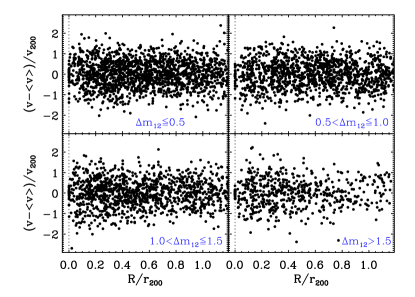
Figure 1: Projected phase-space distribution of galaxies in the four samples. Top-left panel: systems with $\Delta m_{12}\leq 0.5$. Top-right panel: systems with $0.5<\Delta m_{12}\leq 1.0$. Bottom-left panel: systems with $1.0<\Delta m_{12}\leq 1.5$. Bottom-right panel: systems with $\Delta m_{12}>1.5$.

3.1 Stacking the clusters

The number of spectroscopic members in any of the clusters is too small for allowing a robust individual cluster determination of $\beta(r)$, with the exception of Abell 85, already analysed by Aguerri et al. (2017). To improve statistics, we built stacks of clusters in each $\Delta m_{12}$ sample. In our stacking procedure we follow several previous dynamical studies (e.g. van der Marel et al. 2000; Rines et al. 2003; Katgert et al. 2004; Biviano et al. 2016b). The procedure relies on the assumption that different clusters have similar mass profiles, differing only for the normalisation. Such an assumption is justified by the existence of a universal mass profile for cosmological halos (Navarro et al. 1997) and on the fact that the concentration of halo mass profiles is very mildly mass-dependent (e.g. Biviano et al. 2017).

Following Munari et al. (2013), we compute the virial radius $r_{200}=\sigma_{\rm v}/(6.67\,H_{z})$, where $\sigma_{\rm v}$ is the line-of-sight rest-frame velocity dispersion and $H_{z}$ is the Hubble constant at redshift $z$. Only for one system, FGS28, we estimate its virial radius from its X-ray luminosity, $L_{X}$, since it does not contain enough members in its central region for a reliable $\sigma_{v}$ estimate (see note in Table 6 for details). We also compute the virial velocity v${}_{200}=10\,H_{z}\,r_{200}$. We stack the individual clusters by scaling the cluster-centric galaxy distances $R$ to the virial radius, $R/r_{200}$, and the line-of-sight, rest-frame velocities, $\rm{v}_{{\rm rf}}\equiv c\,(z-{\rm<}z{\rm>})/(1+{\rm<}z{\rm>})$, where $c$ is the speed of light and ¡$z$¿ is the cluster mean redshift, to the virial velocity, $\rm{v}_{rf}/\rm{v}_{200}$.

The properties of the four stacks are computed as the weighted averages of the properties of the clusters in each sample, using the number of member galaxies as weights, and are presented in Table 1. The four stacks have very similar mean redshifts, while the mean $r_{200}$ values are marginally different among each others. The projected phase-space distributions of galaxies in the four samples is shown in Fig. 1.

3.2 MAMPOSSt

When the mass profile of a cluster is derived from the kinematics of its galaxies (as in this work) using the Jeans equation (e.g. van der Marel 1994), the solutions for $M(r)$ and $\beta(r)$ are degenerate with respect to the usually adopted osbervables, the projected number-density and velocity-dispersion profiles (e.g. Walker et al. 2009). The MAMPOSSt technique of Mamon et al. (2013) has been shown to partially break this degeneracy. It estimates $M(r)$ and $\beta(r)$ in a parametrised form, by performing a maximum likelihood fit to the full distribution of galaxies in the projected phase space.

In our analysis we consider three models for $M(r)$:

• the Navarro, Frenk, and White profile (NFW, Navarro et al. 1997),

  $$M_{NFW}(r)=M_{200}\frac{{\rm ln}(1+r/r_{-2})-r/r_{-2}(1+r/r_{-2})^{-1}}{{\rm ln}(1+c_{200})-c_{200}/(1+c_{200})},$$ (2)

  where $M_{200}\equiv 100\,H_{z}^{2}\,r_{200}^{3}/G$, and $H_{z}$ is the Hubble constant at the system redshift, $c=r_{200}/r_{-2}$ is the concentration of $M(r)$, and $r_{-2}$ is the scale radius, defined as the radius where the NFW profile has a logarithmic slope of -2 (Navarro et al. 2004).

• The Einasto profile (Einasto 1965; Navarro et al. 2004),

  $$M_{E}(r)=M_{200}\frac{P[3m,2m(r/r_{-2})^{1/m}]}{P[3m,2m(r_{200}/r_{-2})^{1/m}]},$$ (3)

  where $P(a,x)$ represents the regularised incomplete gamma function, and where we fix $m=5$, which represents well cluster-size halos in numerical simulations (Mamon et al. 2010).

• The Burkert profile (Burkert 1995; Biviano et al. 2013),

  $$\begin{split}M_{B}(r)=M_{200}\,\{\ln[1+(r/r_{B})^{2}]+2\ln(1+(r/r_{B})\,-\\ -\,2\arctan(r/r_{B})\}\times\,\{\ln[1+(r_{200}/r_{B})^{2}]\,+\\ +\,2\ln(1+(r_{200}/r_{B})-2\arctan(r_{200}/r_{B})\}^{-1},\end{split}$$ (4)

where $r_{B}$ is the scale radius of the model. All these models have two free parameters, $r_{-2}$ and $r_{200}$. However, the four stacks on which we run MAMPOSSt, have the observables already defined in virial units, $R/r_{200}$ and $\rm{v}_{rf}/\rm{v}_{200}$ (see Sect. 3.1), so $r_{200}$ is no longer a free parameter. In Sect. 4 we show that if we allow $r_{200}$ as a free parameter in the MAMPOSSt analysis, the best-fit values are consistent with the mean values reported in Table 1, and the likelihood of the MAMPOSSt best-fit does not improve significantly with respect to keeping $r_{200}$ fixed.

We consider five different models for $\beta(r)$:

• “C”: constant anisotropy with radius, $\beta=\beta_{c}$.

• “T”: from Tiret et al. (2007),

  $$\beta_{T}(r)=\beta_{\infty}\frac{r}{r+r_{-2}},$$ (5)

  where $\beta_{\infty}$ is the anisotropy value at large radii.

• “O”: from Biviano et al. (2013),

  $$\beta_{O}(r)=\beta_{\infty}\frac{r-r_{-2}}{r+r_{-2}}.$$ (6)

• “ML”: from Mamon & Łokas (2005),

  $$\beta_{ML}(r)=\frac{1}{2}\,\frac{r}{r+r_{\beta}},$$ (7)

  where $r_{\beta}$ is the anisotropy radius.

• “OM”: from Osipkov (1979) and Merritt (1985),

  $$\beta_{OM}(r)=\frac{r^{2}}{r^{2}+r_{\beta}^{2}}.$$ (8)

All these $\beta(r)$ models have one free parameter each ($\beta_{C},\beta_{\infty},$ or $r_{\beta}$).

We run MAMPOSSt in the so-called Split mode (Mamon et al. 2013), that is we use an external maximum-likelihood analysis to determine the value of the scale radius of the galaxies number density profile, $r_{\nu}$. We fit the radial distributions of the galaxies in each stack with NFW models (in projection), taking into account the correction for sample incompleteness as in Zarattini et al. (2019). The best fit values for $r_{\nu}$ are given in Table 1. The $\Delta m_{12}>1.5$ sample has a slightly more concentrated distribution of galaxies than the other three samples.

3.3 Inversion of the Jeans equation

While MAMPOSSt is able to constrain $M(r)$ and $\beta(r)$, the constraints are specific to the set of models that are considered (see the previous Sect.). There is a vast literature on the modelisation of cluster $M(r)$ (e.g. Ludlow et al. 2013; Pratt et al. 2019, and references therein). On the other hand, less is known from numerical simulations and observations about the shape of $\beta(r)$ in galaxy systems, and a large variance among different systems has been suggested (see Fig. 1 in Mamon et al. 2013). Our choice of models for MAMPOSSt could therefore be adequate to describe $M(r)$, but not perhaps to describe $\beta(r)$. To confirm that our $\beta(r)$ modelisation is not too restrictive we use the $M(r)$ determined by the MAMPOSSt analysis, to directly invert the Jeans equation and derive $\beta(r)$ in an (almost) non-parametric way. For this, we follow the method of Binney & Tremaine (1987) in the implementations of Solanes & Salvador-Sole (1990) and Dejonghe & Merritt (1992).

Our procedure is the following. We fix $M(r)$ to the MAMPOSSt solution. The two observables we need to consider are the number density and velocity dispersion profiles. We apply the LOWESS technique (see, e.g., Gebhardt et al. 1994) to smooth these profiles. The number density profile is then de-projected numerically, (using Abel’s equation, see Binney & Tremaine 1987). Since the equations to be solved contain integrals up to infinity, we extrapolate the profiles to a large-enough radius – we find 30 Mpc to be sufficient for our results to be stable. The extrapolations are performed as in Biviano et al. (2013).

Uncertainties in the $\beta(r)$ profiles are estimated by performing the Jeans inversion on 100 bootstrap resamplings of the original datasets.

4 Results

4.1 MAMPOSSt

We apply MAMPOSSt to the four samples of Table 1, limiting each data set to the region $0.05\,\rm{Mpc}\leq R\leq r_{200}$, since the inner region, $R<0.05$ Mpc, is dominated by the BCG, where our parametrisation of $M(r)$ may not work because the total mass is no longer DM-dominated (e.g. Biviano & Salucci 2006), while the outer region, $R>r_{200}$, may not have reached dynamical equilibrium yet.

Table 2: Results.

$\Delta m_{12}$	$M(r)$	$\beta(r)$	$r_{-2}$	$\beta(r_{200}/4)$	$\beta(r_{200})$
	model	model	[Mpc]
(1)	(2)	(3)	(4)	(5)	(6)
MAMPOSSt: minimum BIC
$\leq 0.5$	Einasto	C	$0.8\pm 0.2$	$1.2\pm 0.1$	$1.2\pm 0.1$
0.5–1.0	Einasto	C	$1.0\pm 0.3$	$1.3\pm 0.1$	$1.3\pm 0.1$
1.0–1.5	Einasto	C	$0.7\pm 0.2$	$1.3\pm 0.1$	$1.3\pm 0.1$
$>1.5$	Burkert	T	$0.3\pm 0.1$	$1.4\pm 0.1$	$2.1\pm 0.4$
MAMPOSSt: minimum BIC for NFW models
$\leq 0.5$	NFW	C	$0.7\pm 0.2$	$1.2\pm 0.1$	$1.2\pm 0.1$
0.5–1.0	NFW	C	$0.9\pm 0.2$	$1.3\pm 0.1$	$1.3\pm 0.1$
1.0–1.5	NFW	C	$0.6\pm 0.2$	$1.3\pm 0.1$	$1.3\pm 0.1$
$>1.5$	NFW	T	$0.5\pm 0.1$	$1.3\pm 0.1$	$1.7\pm 0.3$
MAMPOSSt: $\hat{L}$-weighted average of all models
$\leq 0.5$	all	all	$0.6\pm 0.2$	$1.1\pm 0.1$	$1.1\pm 0.1$
0.5–1.0	all	all	$0.7\pm 0.3$	$1.1\pm 0.1$	$1.2\pm 0.1$
1.0–1.5	all	all	$0.6\pm 0.3$	$1.2\pm 0.1$	$1.2\pm 0.1$
$>1.5$	all	all	$0.4\pm 0.2$	$1.3\pm 0.3$	$1.5\pm 0.3$
Jeans equation inversion
$\leq 0.5$	Einasto	none	0.8	$1.1\pm 0.1$	$1.3\pm 0.1$
0.5–1.0	Einasto	none	1.0	$1.5\pm 0.1$	$1.4\pm 0.1$
1.0–1.5	Einasto	none	0.7	$1.4\pm 0.2$	$1.6\pm 0.1$
$>1.5$	Burkert	none	0.3	$1.4\pm 0.2$	$1.9\pm 0.4$

We compare the MAMPOSSt solutions obtained from the 15 combinations of the three $M(r)$ and the five $\beta(r)$ models (see Sect. 3.2) using the Bayesian Information Criterion (BIC Schwarz 1978),

$${\rm BIC}=N_{\rm{pars}}\ln N_{\rm{data}}\,-2\ln(\hat{L}),$$ (9)

where $N_{\rm{data}}$ is the sample size, and $N_{\rm{pars}}$ is the number of free parameters used in the model and $\hat{L}$ is the MAMPOSSt-derived likelihood. The BIC values obtained using two free parameters ($r_{-2},$ and the $\beta(r)$ parameter) are systematically lower than the BIC values obtained using three free parameters (i.e. adding $r_{200}$ as a free parameter) for all combinations of $M(r)$ and $\beta(r)$ models. This means there is no statistical advantage of adding $r_{200}$ as a free parameter in our analysis, presumably because the stack sample observables are already in normalised units with respect to $r_{200}$ and $\rm{v}_{200}$. Anyway, we checked that the best-fit $r_{200}$ values obtained by MAMPOSSt in the 3-free parameters runs, are consistent with the weighted mean values of $r_{200}$ resulting from the cluster stacking procedure (listed in Table 1; see also Sect. 3.1).

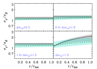
Figure 2: MAMPOSSt estimates of the velocity anisotropy profile, $\sigma_{r}/\sigma_{\theta}$, for the four samples. Black curve and grey shading: minimum-BIC solution and 1 $\sigma$ confidence region estimated by the MCMC analysis. Green dashed curve and turquoise shading: weighted average and dispersion of the MAMPOSSt results from all different combinations of $M(r)$ and $\beta(r)$ models, using the MAMPOSSt likelihoods as weights. See also Table 2. Top-left panel: systems with $\Delta m_{12}\leq 0.5$. Top-right panel: systems with $0.5<\Delta m_{12}\leq 1.0$. Bottom-left panel: systems with $1.0<\Delta m_{12}\leq 1.5$. Bottom-right panel: systems with $\Delta m_{12}>1.5$.

The main results of the MAMPOSSt analysis are given in Table 2. We list the best-fit values of $r_{-2}$ and the values of $\beta(r)$ at two characteristic radii ($r_{200}/4$ and $r_{200}$). These values are listed for the combination of $M(r)$ and $\beta(r)$ models that give the minimum BIC values for each of the four samples. The minimum-BIC solutions for the three smaller $\Delta m_{12}$ samples are obtained using the Einasto mass profile and the constant anisotropy profile. On the other hand, for the $\Delta m_{12}>1.5$ sample the minimum-BIC solution is obtained using the Burkert mass model and the T anisotropy model. The listed uncertainties are marginalised errors obtained from a Markov chain Monte Carlo (MCMC) analysis.

The $\Delta m_{12}>1.5$ sample differs from the other three not only for the different minimum-BIC models, but also for the larger value of $\beta(r_{200})$, and for the smaller value of $r_{-2}$. The smaller $r_{-2}$ implies a higher concentration of the mass distribution, as already found for the galaxy distribution in Sect. 3.2. A higher mass concentration for systems with large magnitude gaps is predicted by cosmological numerical simulations (Ragagnin et al. 2019). However, the smaller $r_{-2}$ we find for $\Delta m_{12}>1.5$ systems probably compensates for the fact that the Burkert mass model is cored at the centre, unlike the Einasto model. In fact, when we force the NFW $M(r)$ model to all the samples, the $r_{-2}$ values of the four samples are not much different (see the second set of results in Table 1). On the other hand, the $\beta(r_{200}$ value of the $\Delta m_{12}>1.5$ sample is larger than the corresponding values of the the other three samples, independently of the $M(r)$ model.

The third set of results shown in Table 2 are the weighted average MAMPOSSt results of all models combinations, using the MAMPOSSt likelihoods $\hat{L}$ as weights. The quoted errors on the parameters are the weighted variance. Also for this set of results, it is confirmed that the $\Delta m_{12}>1.5$ sample has a higher $\beta(r_{200})$ value compared to the other three samples, although the difference is less significant than for the minimum-BIC, and the minimum-BIC NFW sets of results.

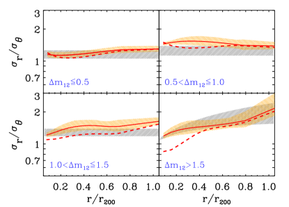
Figure 3: Red solid curves and orange shadings: velocity anisotropy profile $\sigma_{r}/\sigma_{\theta}$ and 1 $\sigma$ confidence regions (estimated from 100 bootstrap resampling) for the four samples, obtained from the Jeans equation inversion using the minimum-BIC MAMPOSSt $M(r)$ (see Table 2). The dashed red curves indicate the solutions obtained including galaxies in the central $<0.05$ Mpc regions. For comparison, the grey shadings reproduce the 1 $\sigma$ confidence regions of the MAMPOSSt solutions shown in Fig. 2. Top-left panel: systems with $\Delta m_{12}\leq 0.5$. Top-right panel: systems with $0.5<\Delta m_{12}\leq 1.0$. Bottom-left panel: systems with $1.0<\Delta m_{12}\leq 1.5$. Bottom-right panel: systems with $\Delta m_{12}>1.5$.

In Fig. 2 we display the four samples velocity anisotropy profiles, $\sigma_{r}/\sigma_{\theta}$, corresponding to the first and third sets of results of Table 2. We do not show the velocity anisotropy models obtained by forcing the NFW $M(r)$ for the sake of clarity of the plot – anyway, they are quite similar to those of the minimum-BIC models. The velocity anisotropy of the $\Delta m_{12}>1.5$ sample is increasing with radius, indicating more radial orbits in the outer regions than the other three samples.

The differences we found are larger than $1\sigma$, but smaller than $3\sigma$. There is therefore only tentative evidence for the presence of more radial orbits in systems with large magnitude gap. A larger data set is needed to provide a more solid statistical basis to our result, and eventually to extend it to a sample of pure fossil systems.

4.2 Jeans equation inversion

Given the best-fit MAMPOSSt $M(r)$ models and the observables, namely the galaxies number-density and velocity-dispersion profiles, we now perform the inversion of the Jeans equation to determine $\beta(r)$ in a non-parametric form. This procedure allows us to free the determination of $\beta(r)$ from the constraints imposed by the choice of models used in the MAMPOSSt analysis. Also in this case we limit the analysis to the region $0.05\,\rm{Mpc}\leq R\leq r_{200}$.

The results of the Jeans inversion analysis are shown in Fig. 3. The results are similar to those obtained with MAMPOSSt. The marginal differences (always within 20%) between the $\sigma_{r}/\sigma_{\theta}$ profiles obtained by the two methods can be attributed to the limited number of $\beta(r)$ models considered in MAMPOSSt.

There appears to be a trend of increasing $\beta(r)$ at large radii with increasing $\Delta m_{12}$. This is confirmed by the values of $\beta(r_{200})$ reported in Table 2.

Near the centre, the situation is less clear. To better investigate the inner region, we repeat the Jeans inversion analysis by extending the analysed region to $0.0\leq R\leq r_{200}$. The results are shown in Fig. 3 (dashed lines). Including the galaxies near the centre leads to decreasing velocity anisotropy near the centre in all samples, but the decrease is stronger in the systems with higher $\Delta m_{12}$. A possible explanation for this behaviour resides in the velocity segregation of BCGs that is stronger for systems with higher $\Delta m_{12}$, as found by Zarattini et al. (2019). Dynamical friction can decrease the velocities of galaxies but also make their orbits more isotropic if not tangential.

4.3 Systematics

Here we examine possible systematics affecting our result.

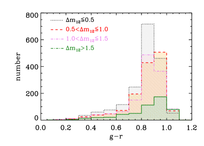
Figure 4: $g-r$ colour distribution of the galaxies in the four samples. Dotted black histogram and grey shading: $\Delta m_{12}\leq 0.5$. Dashed red histogram and orange shading: $0.5<\Delta m_{12}\leq 1.0$. Dash-dotted violet histogram and pink shading: $1.0<\Delta m_{12}\leq 1.5$. Solid green histogram and turquoise shading: $\Delta m_{12}>1.5$.

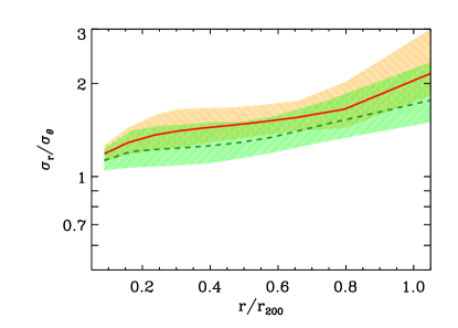
Figure 5: Velocity anisotropy profile $\sigma_{r}/\sigma_{\theta}$ and 1 $\sigma$ confidence regions for the systems with $\Delta m_{12}>1.5$. Solid red line and orange shading: based on all 20 systems (same as bottom-right panel in Fig. 3); dashed green line and green shading: based on 17 systems, excluding the three richest.

In low-$z$ clusters, late-type/blue galaxies are observed to have more radially anisotropic orbits than early-type/red galaxies (Biviano & Katgert 2004; Munari et al. 2013; Mamon et al. 2019, e.g.). If the $\Delta m_{12}>1.5$ systems contain a a larger fraction of late-type/blue galaxies compared to the systems that compose the other three samples, this could explain the higher values of $\beta$ at large radii.

Lacking detailed studies of galaxy populations as a function of $\Delta m_{12}$ in the literature, we here determine the galaxies $g-r$ colour distribution in the four stacks. These are shown in Fig. 4. It can be seen that systems in the $\Delta m_{12}>1.5$ bin do not show a larger amount of late-type/blue galaxies. If anything, they contain more red galaxies, mostly because of the deep spectroscopic follow-up of the S1 data set, that contributes most systems in the $\Delta m_{12}>1.5$ bin. The S1 data set includes many dwarf galaxies, up to three magnitudes fainter than SDSS spectroscopy. Dwarf galaxies in clusters/groups are mostly early-type (e.g. Jerjen & Tammann 1997; Lisker et al. 2013), and therefore occupy the red tail of the $g-r$ distribution.

Different $\beta(r)$ have also been reported for galaxies of different stellar masses (Annunziatella et al. 2016) or luminosity (Aguerri et al. 2017). To check if a different magnitude distribution could be at the origin of the different $\beta(r)$ seen for the $\Delta m_{12}>1.5$ stack, we repeat the MAMPOSSt analysis using only galaxies with $r\leq 17.77$. This is the magnitude limit of the SDSS spectroscopy, and effectively exclude the tail of red dwarf galaxies from the two highest-$\Delta m_{12}$ samples, while leaving almost unchanged the other two samples. We find that the results for the $\beta(r)$ of the four stacks do not change significantly when applying the magnitude cut $r\leq 17.77$, with $\beta(r_{200})$ changing by $<5$%.

The number of members is very different in different systems of our data set. To check that our result is not driven by a few very rich systems, we removed from the $\Delta m_{12}>1.5$ sample the three richest clusters, FGS03, FGS27 and FGS30 that together contain almost 1/3 of all members in their sample (see Table 6). We performed the full analysis on the remaining sample of 17 systems. The resulting $\sigma_{r}/\sigma_{\theta}$ profile is very similar to the original one based on all 20 systems (see Fig. 5).

The S1 and S2 data sets cover different $z$ ranges, their median $z$ are 0.16 and 0.07, respectively. This difference reflects in an increase of the ¡$z$¿ of the four samples with increasing $\Delta m_{12}$, since the higher-$\Delta m_{12}$ systems are mostly from the S1 data set. To check for a $z$-dependence of $\beta(r)$ we divided our $\Delta m_{12}>1.5$ sample in two subsamples, of ten clusters at $z<0.12$ and another ten at $z>0.12$. After performing the dynamical analysis separately on the two subsamples, we found no significant difference in their $\beta(r)$, but the uncertainties are large due to the small size of the subsamples, so this test cannot be considered very significant.

There is independent support against the hypothesis that the ¡$z$¿ difference across the four samples can be the reason for the observed difference in $\beta(r)$. The ¡$z$¿ range across the four samples correspond to 0.7 Gyr in cosmic time. This is only 25% of the dynamical time for a typical system of galaxies at $z\sim 0.1$ (Sarazin 1986), and it is unlikely that galaxies could modify their orbits in such a short time. Moreover, there is no observational evidence for orbital evolution of cluster galaxies across the much larger cosmic time span from $z=1.32$ to $z=0.26$ (corresponding to 6 Gyr, Capasso et al. 2019b).

5 Discussion and conclusions

We analysed a data set of 97 galaxy clusters and groups to study the dependence of $\beta(r)$, and therefore of the orbital distribution of galaxies, on $\Delta m_{12}$. We split our data set in four samples of different $\Delta m_{12}$. We then stacked together the systems in each of the four samples. We then run MAMPOSSt to derive the mass and the (parametric) anisotropy profiles of the four samples. Finally, with the mass profiles obtained from MAMPOSSt, we perform the inversion of the Jeans equation, allowing us to determine $\beta(r)$ in a model-independent way.

We find that $\beta(r)$ shows a steeper dependence on $r$ for the systems with $\Delta m_{12}>1.5$ than for the other three samples with smaller $\Delta m_{12}$. The orbits of galaxies in the $\Delta m_{12}>1.5$ stack are more radial (with marginal significance, at more than $1\sigma$ level) at large radii ($r\gtrsim 0.8\,r_{200}$) than in systems with smaller $\Delta m_{12}$. In the central regions the orbits of galaxies are nearly isotropic in all stacks, or even tangential at radii $<0.05$ Mpc in the $\Delta m_{12}>1.5$ stack. The tangential orbits found in the very central regions of these systems are related to the observed velocity segregation (Zarattini et al. 2019) in the same region, and can be interpreted as an effect of dynamical friction slowing down galaxies that approach their cluster centre.

Dynamical friction is thought to be more efficient for galaxies on radial orbits (Lacey & Cole 1993). As galaxies lose their kinetic energy due to dynamical friction, they can more easily merge with the central galaxy, and this is the process suggested by Sommer-Larsen et al. (2005) for the formation of large magnitude gaps in galaxy systems.

In Zarattini et al. (2015) we studied the dependence of the luminosity function (LF) on the magnitude gap. We found that systems with $\Delta m_{12}>1.5$ are missing not only L${}^{*}$, but also dwarf galaxies. In fact, the faint end of their LFs is clearly flatter than that of $\Delta m_{12}<1.5$ systems. Moreover, Adami et al. (2009) found that dwarf galaxies in Coma are located in radial orbits even in the central region of the cluster. Thus, we suggest that also the lack of dwarf galaxies in FGs could be linked to radial orbits. Unfortunately, deeper data are required to study the orbits of dwarf galaxies in FGs, studies that could be done in the near future with new wide-field spectroscopic facilities (e.g. the WEAVE spectrograph).

Galaxy systems are thought to evolve from an initial phase of rapid collapse characterised by isotropisation of galaxy orbits, to a phase of slow accretion characterised by radial orbits (Lapi & Cavaliere 2011). Major mergers operate in the same way as the initial phase of rapid collapse, introducing dynamical entropy in the system, and transferring angular momentum from clusters colliding off-axis to galaxies, leading to orbit isotropisation. The fact that $\Delta m_{12}>1.5$ systems have more galaxies on radial orbits than smaller-$\Delta m_{12}$ systems therefore suggests a difference in the time since last major merger, and this supports the conclusions of Kundert et al. (2017) based on cosmological simulations.

However, although D’Onghia et al. (2005) found that radial orbits are required for the formation of FGs (see their Eq. 3), there is no clear evidence of correlation between the type of orbits and the magnitude gap in numerical simulations. Our observational confirmation of the presence of radial orbits in systems with large magnitude gaps could be a boost for the analysis of future simulations in order to explain such a difference.

In summary, our study is a first observational confirmation that galaxies in systems with large $\Delta m_{12}$ have more radially elongated orbits than galaxies in systems with small $\Delta m_{12}$. Our samples contain a mix of pure FGs and normal systems. A substantial increase of the spectroscopic data set for FGs is needed to check if our results also apply for these systems as a separated class.

Appendix A Sample properties

Here we present the main properties for the four samples of systems with different $\Delta m_{12}$. Some of them were already published in Zarattini et al. (2014) and Aguerri et al. (2007), respectively.

Table 3: Global properties of the $\Delta m_{12}\leq 0.5$ sample.

Name	R.A.	Dec	$N_{m}$	z	$r_{200}$	$\Delta m_{12}$
					[Mpc]
ABELL2092	233.333000	31.212000	45	0.067	0.95	0.00
ZwCl1316.4-0044	199.807000	-0.987810	39	0.083	1.14	0.01
ABELL1452	180.780000	51.675200	25	0.062	1.10	0.06
ABELL1142	165.239000	10.505500	61	0.035	1.17	0.07
ABELL1270	172.175000	54.172300	52	0.069	1.17	0.09
RXJ1053.7+5450	163.402000	54.868000	61	0.072	1.37	0.09
ZwCl1730.4+5829	261.862000	58.516500	47	0.028	1.03	0.12
ABELL2169	243.550000	49.120300	49	0.058	1.08	0.14
FGS06	131.235964	42.976592	28	0.054	0.75	0.20
ABELL1003	156.257000	47.841900	31	0.063	1.28	0.22
ABELL1066	159.778000	5.209770	98	0.069	1.71	0.23
ABELL1205	168.334000	2.546670	83	0.076	1.83	0.25
WBL238	146.689000	54.426900	67	0.047	1.26	0.27
ABELL0757	138.282000	47.708400	40	0.051	0.85	0.33
ABELL2149	240.367000	53.947400	34	0.065	0.95	0.33
ABELL0602	118.361000	29.359500	83	0.061	1.73	0.35
ABELL2018	225.283000	47.276600	44	0.087	1.30	0.35
MACSJ0810.3+4216	122.597000	42.273900	41	0.064	1.05	0.35
RXCJ0137.2-0912	24.314100	-9.197610	46	0.041	0.95	0.35
RXCJ1424.8+0240	216.198000	2.664440	20	0.054	1.12	0.37
FGS09	160.760712	0.905070	67	0.125	1.73	0.40
ABELL1436	179.860000	56.403700	86	0.065	1.47	0.41
ZwCl1215.1+0400	184.421000	3.655840	129	0.077	1.96	0.41
ABELL1616	191.851000	54.987000	42	0.083	1.16	0.42
ABELL1552	187.548000	11.743800	17	0.088	0.90	0.44
ABELL1507	183.703000	59.906200	42	0.060	0.79	0.45
ABELL1016	156.782000	11.010700	27	0.032	0.54	0.46
ABELL1885	213.431000	43.644800	23	0.089	1.11	0.47
ABELL2255	258.120000	64.060800	267	0.080	1.81	0.47
RXCJ1121.7+0249	170.386000	2.887250	68	0.049	1.18	0.47
ZwCl0743.5+3110	116.637000	31.022700	31	0.058	1.44	0.47

Table 4: Global properties of the $0.5<\Delta m_{12}\leq 1.0$ sample.

Name	R.A.	Dec	$N_{m}$	z	$r_{200}$	$\Delta m_{12}$
					[Mpc]
ABELL1630	192.973000	4.579790	32	0.065	0.92	0.51
ABELL1999	223.511000	54.265700	36	0.099	0.94	0.54
ABELL0819	143.071000	9.683590	31	0.076	1.10	0.55
ABELL1783	205.735000	55.603900	46	0.069	0.79	0.59
ABELL2023	227.497000	3.003090	25	0.092	1.05	0.60
ABELL0628	122.535000	35.275300	54	0.084	1.37	0.67
ABELL1516	184.718000	5.245670	66	0.077	1.48	0.68
ABELL1809	208.277000	5.149730	90	0.079	1.51	0.72
ZwCl0027.0-0036	7.368420	-0.212620	35	0.060	0.96	0.72
ABELL1424	179.371000	5.089060	72	0.076	1.27	0.73
ABELL1728	200.882000	11.302200	49	0.090	1.68	0.73
ABELL1620	192.516000	-1.540380	58	0.085	1.70	0.74
ABELL1169	167.096000	44.150300	41	0.058	0.90	0.79
NSCJ161123+365846	242.808000	36.973400	44	0.067	1.00	0.83
RXJ1022.1+3830	155.656000	38.579200	62	0.054	1.23	0.83
WBL518	220.178000	3.465420	109	0.027	0.96	0.85
ABELL1149	165.740000	7.603880	28	0.072	0.73	0.90
ABELL2175	245.130000	29.891000	78	0.096	1.79	0.90
ABELL1346	175.299000	5.734720	77	0.098	1.61	0.91
ABELL0971	154.967000	40.988500	41	0.093	1.67	0.97
ABELL1663	195.719000	-2.517850	80	0.083	1.49	0.97
ABELL0168	18.740000	0.430810	105	0.045	1.21	0.98
ABELL2670	358.557000	-10.419000	143	0.076	1.32	0.99

Table 5: Global properties of the $1.0<\Delta m_{12}\leq 1.5$ sample.

Name	R.A.	Dec	$N_{m}$	z	$r_{200}$	$\Delta m_{12}$
					[Mpc]
ABELL1767	204.035000	59.206400	148	0.071	1.83	1.01
ABELL2241	254.933000	32.615300	38	0.098	1.64	1.02
FGS31	260.041836	38.834513	120	0.159	2.30	1.04
ABELL0695	130.305000	32.416600	20	0.068	0.94	1.05
ABELL0085	10.460300	-9.303130	271	0.055	2.03	1.09
ABELL2245	255.638000	33.516700	44	0.086	1.10	1.09
ABELL1750	202.711000	-1.861970	41	0.088	1.06	1.11
FGS25	234.961581	48.404745	117	0.097	1.67	1.12
ABELL0257	27.285000	13.963300	28	0.070	0.79	1.14
NSCJ152902+524945	232.311000	52.863900	54	0.074	1.34	1.16
FGS26	237.232728	44.134516	83	0.072	0.95	1.18
ABELL0724	134.541000	38.640400	30	0.094	0.88	1.20
FGS13	175.367899	10.823113	18	0.188	1.27	1.23
ABELL1564	188.758000	1.798650	53	0.079	1.32	1.25
ABELL2244	255.690000	34.061100	26	0.096	0.87	1.26
RXCJ1115.5+5426	168.849000	54.444100	60	0.070	1.32	1.28
ABELL0779	139.945000	33.749700	59	0.023	0.71	1.34
FGS19	203.999933	41.527137	27	0.177	1.48	1.35
MACSJ1440.0+3707	220.014000	37.124300	19	0.098	1.19	1.36
ABELL2428	334.065000	-9.333250	32	0.084	0.89	1.38
ABELL0152	17.513200	13.978200	38	0.060	1.12	1.40
RXCJ1351.7+4622	208.161000	46.349800	59	0.063	1.10	1.40
FGS22	223.495881	-3.524771	31	0.146	0.92	1.49

Table 6: Global properties of the $\Delta m_{12}>1.5$ sample.

Name	R.A.	Dec	$N_{m}$	z	$r_{200}$	$\Delta m_{12}$
					Mpc
RBS1385	215.965000	40.258800	17	0.082	0.86	1.60
FGS12	170.480324	40.626439	26	0.240	1.43	1.61
FGS27	243.629598	30.717775	76	0.184	1.37	1.61
FGS04	121.878105	34.011550	28	0.208	1.58	1.65
ABELL0117	13.966200	-9.985650	57	0.055	1.10	1.69
ZwCl1207.5+0542	182.570000	5.386040	42	0.077	1.19	1.69
FGS29	251.758645	26.730653	27	0.135	0.96	1.81
FGS34	359.562947	56.665593	35	0.178	1.07	1.82
FGS30	259.549773	41.188995	71	0.114	1.64	1.84
ABELL0999	155.849000	12.835000	25	0.032	0.57	1.86
FGS23	232.442800	41.755800	63	0.148	1.08	1.87
ABELL2110	234.962000	30.717800	25	0.098	1.27	1.88
FGS14	176.698219	5.974865	39	0.221	1.59	1.96
FGS17	191.925308	9.874491	14	0.155	0.92	1.96
RXCJ0953.6+0142	148.422000	1.700650	25	0.098	1.19	1.97
FGS03	118.184160	45.949280	102	0.052	1.03	2.09
FGS02	28.174836	1.007103	45	0.230	2.07	2.12
FGS20	212.517450	44.717033	29	0.094	0.79	2.17
ABELL0690	129.816000	28.844100	27	0.079	0.81	2.30
FGS28	249.335485	8.845654	19	0.032	0.47*	3.28

*$r_{200}$ estimated using $L_{X}$, since FGS28 has only one member within the virial radius. We firstly estimated $r_{500}$ by using Eq. 2 from Böhringer et al. (2007), then convert it to $r_{200}$ by using $r_{200}=1.516\,r_{500}$, according to Arnaud et al. (2005). See Girardi et al. (2014) for details.