HARP-Net: Hyper-Autoencoded Reconstruction Propagation
for Scalable Neural Audio Coding

Abstract

We propose a novel autoencoder architecture that improves the architectural scalability of general-purpose neural audio coding models. An autoencoder-based codec employs quantization to turn its bottleneck layer activation into bitstrings, a process that hinders information flow between the encoder and decoder parts. To circumvent this issue, we employ additional skip connections between the corresponding pair of encoder-decoder layers. The assumption is that, in a mirrored autoencoder topology, a decoder layer reconstructs the intermediate feature representation of its corresponding encoder layer. Hence, any additional information directly propagated from the corresponding encoder layer helps the reconstruction. We implement this kind of skip connections in the form of additional autoencoders, each of which is a small codec that compresses the massive data transfer between the paired encoder-decoder layers. We empirically verify that the proposed hyper-autoencoded architecture improves perceptual audio quality compared to an ordinary autoencoder baseline.

Index Terms—  audio coding, deep learning, U-Net, autoencoders

1 Introduction

Data compression is an essential aspect of information and communication systems nowadays. Its main aim is to reduce the bitrate by eliminating the redundancy of the data present in the signal by mapping the raw data samples in the original high precision representation (e.g., single-precision floating points) into a compact discrete representation (e.g., a bitstring). In this work, we focus on the audio coding applications where the reconstructed signal on the receiver side is allowed to have reconstruction error once its perceptual quality is above the desired level. While in speech communication low bitrate codecs can achieve the common intelligibility goal, as for music signals, the required bitrate tends to be much higher since the user’s listening experience can be deteriorated even by a subtle perceptual degradation. Hence, scalability to various use cases and bitrates is an important goal in modern speech or audio codecs, such as in unified speech and audio coding (USAC) [1, 2].

With the recent breakthrough in deep learning, neural speech coding emerged as a new research area. Despite their higher computationally complexity than the conventional speech codecs, such as AMR-WB [3] and Opus [4], neural speech codecs show merits in terms of coding gain. For example, fully-convolutional autoencoders have been successfully transformed into a codec, whose bottleneck layer is quantized to produce bitstings out of waveforms [5]. These relatively compact waveform codecs start to compete with AMR-WB and Opus after being coupled with linear predictive coding (LPC) [6]. Meanwhile, generative models, such as WaveNet [7], have proven to be effective towards speech coding reducing bitrates down to 2.4kbps, while retaining reasonable speech quality [8, 9]. In return, the system is burdened by the complex WaveNet-based decoders. A more recent approach proposed to use LPCNet [10], achieving as low as 1.6kbps [11]. Likewise, neural speech coding has advanced by encompassing traditional technology.

However, most promising advancements have been made for speech coding rather than general-purpose audio coding. For example, the WaveNet decoder is designed for very low bitrate cases, while it is too heavy for real-time decoding, e.g., for on-device music players. Meanwhile, the autoencoder-based waveform codecs display significant drawback as they rely on objective loss functions, e.g., the mean-squared error, which often result in perceptual discrepancy among decoded signals. Hence, perceptually more meaningful loss functions show promising results for neural audio coding by calibrating the loss with a psychoacoustic weighting scheme [12]. In [12], the idea of cascading multiple autoencoders [13] also show performance improvement, while the concatenation linearly increases model complexity.

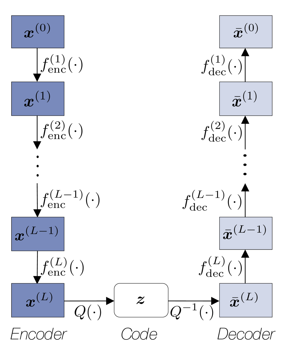
(a) The baseline autoencoder

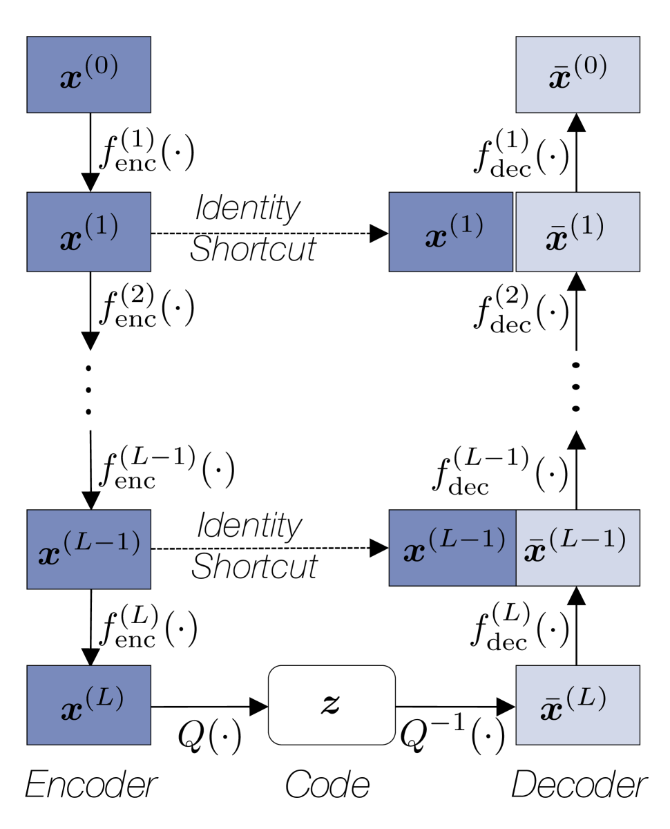
(b) A hypothetical U-Net codec

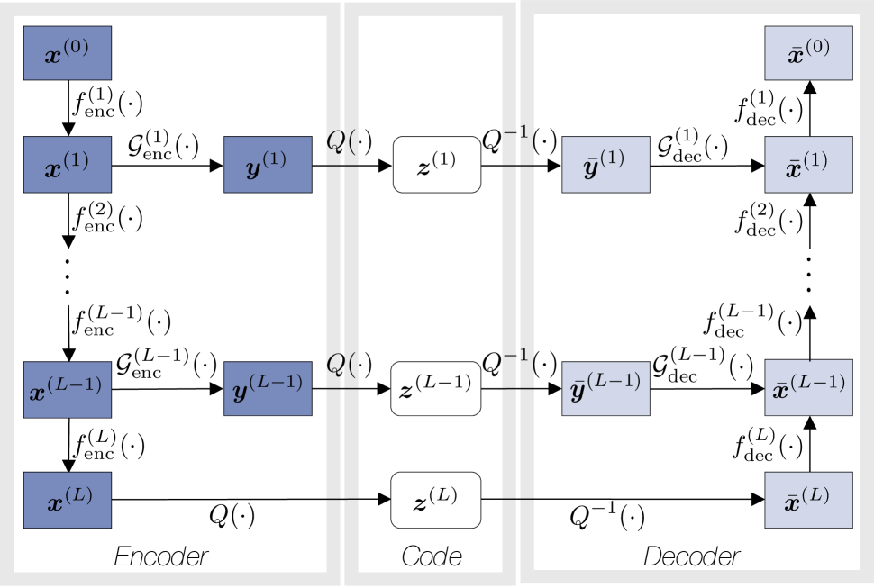
(c) The proposed HARP-Net architecture

Figure 1: The neural audio coding systems discussed in this work. Note that in the hypothetical U-Net codec each identity shortcut requires a substantial bitrate as each $\bm{x}^{(l)}$ is part of code. HARP-Net compresses them further and reduces the total bitrate.

Our proposed method tackles the neural audio coding problem via architectural improvement. Our codec covers various bitrates, while its complexity is suppressed to be low. To this end, we posit a mirrored autoencoder (AE) architecture, where the feature maps on the decoder side are an approximation of the encoder’s. Hence, we conjecture that direct communication between each pair of encoder and decoder layers can improve the layer-wise approximation quality of the decoder. Then, the better approximation performance is propagated to the decoder’s output layer, leading to a better total reconstruction. To this end, we employ additional autoencoding paths that skip-connect the corresponding feature map pairs on the opposite sides. Since each skip AE is a small codec producing a code from its own bottleneck layer, the final bitstream is the sum of all codes from those bottleneck layers. We call the proposed architecture hyper-autoencoded reconstruction propagation network (HARP-Net). HARP-Net shares the similar advantage introduced by the U-Net’s skip connections [14]: a superior reconstruction quality for autoencoding-like tasks, such as music source separation in Wave-U-Net [15]. The difference is that U-Net’s identity shortcuts disqualify the architecture as a codec due to the high datarate. HARP-Net replaces the bitrate-consuming identity shortcuts with compact AEs, whose goal is to deliver the encoder feature map in a compressed form to the decoder side.

2 Neural Audio Coding

2.1 Basic Autoencoders

Figure 1(a) depicts an AE-based neural audio coding system. Its encoder function ${\mathcal{F}}_{\text{enc}}(\cdot)$ converts the input signal into a feature vector, which is subsequently quantized into a bitstring, or the code $\bm{z}$. Compression is achieved if $\bm{z}$ is with a smaller number of bits than the amount necessary to represent the raw input. The decoder ${\mathcal{F}}_{\text{dec}}(\cdot)$ follows to recover the original signal out of the code vector $\bm{z}$. Hence, the AE’s goal is to best predict the reconstruction $\bar{\bm{x}}$ that approximates the input $\bm{x}$ using a short enough bitstring $\bm{z}$. We write this procedure by employing a quantizer $Q$ and its inversion:

$$\bm{x}\approx\bar{\bm{x}}\leftarrow{\mathcal{F}}_{\text{dec}}\circ Q^{-1}(\bm{z}),\quad\bm{z}\leftarrow Q\circ{\mathcal{F}}_{\text{enc}}(\bm{x}).$$ (1)

Neural coding systems employ a deep neural network (DNN) to implement the autoencoding function. Hence, the encoder function ${\mathcal{F}}_{\text{enc}}(\cdot)$ can be defined as a series of non-linear transforms, whose $l$-th layer converts its input $\bm{x}^{(l-1)}$ into a new feature space $\bm{x}^{(l)}$:

$$\bm{z}\leftarrow{\mathcal{F}}_{\text{enc}}(\bm{x})=Q\circ f_{\text{enc}}^{(L)}\circ\cdots\circ f_{\text{enc}}^{(2)}\circ f_{\text{enc}}^{(1)}(\bm{x}),$$ (2)

where $L$ denotes the number of the encoder layers. Hence, we can also denote the raw input as $\bm{x}=\bm{x}^{(0)}$. The encoder output $\bm{x}^{(L)}$ goes through a quantization module $Q$ that discretizes the floating-point feature vector $\bm{x}^{(L)}$ into a bitstring $\bm{z}$. Furthermore, $\bm{z}$ is losslessly compressed by using entropy coding, e.g., Huffman coding.

The de-quantization process $Q^{-1}(\bm{z})$ reverts the code vector $\bm{z}$ back to the floating-point feature $\bar{\bm{x}}^{(L)}$ with a certain amount of quantization error, i.e., $\bar{\bm{x}}^{(L)}$ approximates $\bm{x}^{(L)}$. Then, a series of decoder layers recover the raw signal:

$$\bar{\bm{x}}^{(0)}\leftarrow{\mathcal{F}}_{\text{dec}}(\bm{x})=f_{\text{dec}}^{(1)}\circ\cdots\circ f_{\text{dec}}^{(L-1)}\circ f_{\text{dec}}^{(L)}\circ Q^{-1}(\bm{z}).$$ (3)

Note that layer indices decrease from the bottleneck to the output layer.

Although it is not common in the recent deep learning literature, a hard association between the encoder and decoder layers was popular in some earlier models. For example, in the restricted Boltzmann machines (RBM) [16], we write the $l$-th layer transform $\bm{x}^{(l)}\!\leftarrow\!\bm{W}_{\text{enc}}^{(l)}\bm{x}^{(l-1)}+\bm{b}_{\text{enc}}^{(l)}$. Then, its corresponding decoder layer is defined with the encoder weight matrix $\bm{W}_{\text{enc}}^{(l)}$, but by transposing it: $\bar{\bm{x}}^{(l-1)}\!\leftarrow\!\left(\bm{W}_{\text{enc}}^{(l)}\right)^{\top}\bar{\bm{x}}^{(l)}+\bm{b}_{\text{dec}}^{(l)}$. Since the transpose operation is equivalent to matrix inversion for orthonormal matrices, this association loosely implies an inversion relationship.

The basic AE in Figure 1(a) is with a mirrored architecture, while the coupling of the encoder and decoder layers is not assumed. In the proposed HARP-Net architecture, we postulate the ties between the encoder-decoder layers must be helpful for coding, although the coupling is indirect using skip connections rather than inversion.

2.2 Quantization and Bitrate Control

The quantization function $Q$ maps a floating-point value $x^{(L)}_{i}$ to a pre-defined, finite set of quantization bins. Instead of post-training quantization, we include $Q$ and $Q^{-1}$ as part of the AE, so training of the AE can also suppress the quantization artifact. Since $Q$ is not a differentiable process, we employ soft-to-hard quantization [17], which softens the bin assignment during training. First, it estimates the probability of assigning $i$-th code to $j$-th bin, $\bm{P}=\text{softmax}(\alpha\bm{S})$, where $S_{ij}$ defines the similarity (e.g. negative absolute difference) between $i$-th code value and $j$-th representative $\mu_{j}$. $\alpha$ controls the “hardness” of the logits, i.e., the smaller the softer. The softmax function turns the $i$-th similarity values $\bm{S}_{i:}$ to all $J$ quantization bins into a probability vector $\bm{P}_{i:}$. Then, the convex combination of the soft assignment probability and bin representatives recovers the feature vector: $\tilde{x}^{(L)}_{i}=\sum_{j=1}^{J}P_{ij}\mu_{j}$. The decoder takes $\tilde{\bm{x}}^{(L)}$ as input. This whole process is differentiable.

Conversely, the test-time inference uses the hard quantization. First, from $\bm{S}$, the closest bin index for all scalar codes forms the discrete code $\bm{z}$, i.e., $j^{*}=\operatornamewithlimits{\arg\max}_{j}\bm{S}_{ij}$. Note that we reduce the gap between the soft and hard assignments by annealing $\alpha$, i.e., by gradually increasing it during training: $\lim_{\alpha\rightarrow\infty}\tilde{\bm{x}}^{(L)}=\bar{\bm{x}}^{(L)}$.

The code $\bm{z}$ is further compressed via Huffman coding losslessly, the entropy of $p(x^{(L)}_{i})$ serves as the lower bound of the bitrate, which is unknown. As an alternative, we predict the overall frequency of $j$-th bin being selected, $p_{j}$, by observing the soft assignment probability $\bm{P}$ for all training examples. Hence, the approximate entropy is ${\mathcal{H}}=-\sum_{j}p_{j}\log p_{j}$, which we regularize during training to control the bitrate. For example, the encoder adjusts the distribution of $\bm{x}^{(L)}$, so its entropy matches the target entropy, i.e., the lower bound of the per-frame bitrate.

2.3 The Hypothetical Codec with the U-Net Architecture

In the original U-Net [14] and its variants for audio processing [15, 18] skip connections pair up the encoder and decoder layers through identity shortcuts to improve the AE’s reconstruction performance. Hence, the encoder feature maps are delivered to the decoder layers intact. Figure 1(b) depicts a hypothetical U-Net architecture for neural coding, whose decoder layer now takes as input both the corresponding encoder and decoder feature maps by concatenating them together along the channel dimension:

$$\bar{\bm{x}}^{(l-1)}\leftarrow f_{\text{dec}}^{(l)}\left(\big{[}\bm{x}^{(l)},\bar{\bm{x}}^{(l)}\big{]}\right).$$ (4)

The performance gain entailed by these identity shortcuts is without question. In addition to the information decoded from the binary code vector $\bm{z}$, the decoder layer directly utilizes the encoder feature maps, which can be regarded as less abstract feature representations. However, it is an unrealistic coding system since each identity shortcut consumes a significant amount of bits.

3 The Proposed HARP-Net Architecture

We address the hypothetical U-Net codec’s high data rate issue by replacing the identity shortcuts with additional AEs, which we call skip autoencoders. These skip connections can still be considered a way to provide less processed, i.e., rawer information to the decoder as in U-Net. In this view, since a decoder feature map $\bar{\bm{x}}^{(l)}$ is an approximation of its corresponding encoder representation $\bm{x}^{(l)}$, information coming directly from the encoder will help its reconstruction job. In neural coding, these skip connections can compensate the quantization artifact introduced in the bottleneck layer, i.e., $\bm{z}\leftarrow Q(\bm{x}^{(L)})$, which propagates to all decoder layers.

HARP-Net employs layer-wise skip AEs ${\mathcal{G}}^{(l)}$ to compress the data transferred through U-Net’s skip connections:

$$\bm{x}^{(l)}\approx\bar{\bm{x}}^{(l)}\leftarrow{\mathcal{G}}_{\text{dec}}^{(l)}\circ Q^{-1}(\bm{z}^{(l)}),\quad\bm{z}^{(l)}\leftarrow Q\circ{\mathcal{G}}_{\text{enc}}^{(l)}(\bm{x}^{(l)}).$$ (5)

Now a skip connection is divided into its own encoder ${\mathcal{G}}_{\text{enc}}^{(l)}(\cdot)$ and decoder ${\mathcal{G}}_{\text{dec}}^{(l)}(\cdot)$ parts. Hence, instead of transmitting $\bm{x}^{(l)}$ directly, a skip AE compresses it down to $\bm{z}^{(l)}$, a layer-specific code vector. To this end, first, the encoder defines a feature transformation function $\bm{y}^{(l)}\leftarrow{\mathcal{G}}_{\text{enc}}^{(l)}(\bm{x}^{(l)})$, which produces a a processed version of the original feature map. $\bm{y}^{(l)}$ is followed by the ordinary quantization and Huffman coding that construct the layer-wise bitstring $\bm{z}^{(l)}$. Here, the encoder function ${\mathcal{G}}_{\text{enc}}^{(l)}(\cdot)$ is a placeholder: it can employ any adequate structure, probably with multiple layers. De-quantization recovers $\bar{\bm{y}}^{(l)}$ from $\bm{z}^{(l)}$. Then, the decoder recovers the feature map $\bm{x}^{(l)}\approx\bar{\bm{x}}^{(l)}\leftarrow{\mathcal{G}}_{\text{dec}}^{(l)}(\bar{\bm{y}}^{(l)})$

Once again, the goal here is to recover the original feature $\bm{x}^{(l)}$ with little information loss, using only few bits to represent $\bm{z}^{(l)}$. The final code of the entire system is defined by concatenating all layer-wise codes including the ordinary bottleneck code at $L$-th layer: $\bm{z}=[\bm{z}^{(L)};\bm{z}^{(L-1)};\cdots\bm{z}^{(1)}]$.

HARP-Net’s advantage can be summarized as follows:

• Performance: The additional skip connections boost the reconstruction quality on the decoder side than a single bottleneck code.

• Scalability: Having $\bm{z}^{(L)}$ as the most abstract form of representation, it is natural to perform scalable coding by employing $M$ additional skip AEs as neeeded, i.e., $\bm{z}=[\bm{z}^{(L)};\bm{z}^{(L-1)};\cdots\bm{z}^{(L-M)}]$. $M$ can control the bitrates.

• Flexibility: The proposed method can be applied to any DNN with a mirrored autoencoding architecture. Furthermore, the skip AE’s architecture is open to various choices.

Models	# Layers	# Filters	# Params.
Baseline 1	10	30	218k
HARP-Net (1 Skip AE)	12	24	216k
Baseline 2	9	36	275k
HARP-Net (2 Skip AEs)	12	24	257k
Baseline 3	10	36	315k
HARP-Net (3 Skip AEs)	12	24	298k
Baseline 4	10	38	350k
HARP-Net (4 Skip AEs)	12	24	340k

Table 1: The network topology of variant HARP-Net versions with a varying number of skip AEs. Their associated plain AE baselines are presented with a matching number of parameters. The number of layers do not include the skip AEs while the number of parameters take them into account.

4 Experiments

4.1 The Experimental Setup

We assess the performance of HARP-Net on musical signals. To this end, we use $6,000$ commercially released songs of 13 genres, totalling $5.5$ hours of audio data, which is divided into $5,700$ and $300$ songs for training and validation, respectively. $16$ songs are set aside as a test set. All signals are in mono with a sampling rate of $44.1$kHz. We use a frame size of 16384 with a hop size 32 samples.

The proposed HARP-Net codec operates in two target bitrate setups, 24kbps and 48kbps, but they are defined in the LPC residual domain. To this end, the corresponding LPC coefficients need to be accounted for in the final system bitrate, which amount to 16kbps. Eventually, the resulting bitrates are 40kbps and 64kbps. We opt to remain in relatively high bitrates as we limit our experiment to 44.1kHz signals. We leave lower bitrate cases for future work.

In order to assess the impact of the proposed skip AEs, we train multiple model variants that are with varying number of skip AEs from $M=1$ to $4$. For a fair comparison, we assess each of the HARP-Net models against a vanilla AE with matching number of parameters. Table 1 summarizes the various models trained for our experiments. Note that HARP-Net consists of 12 layers, each of which is with 24 1-d convolutional kernels of size $1\times 15\times 24$. The exception is the final encoder layer, where only one kernel is used to collapse the 24 channels down to 1. Eventually, the dimension of the input frame and encoder output are the same, i.e., $\bm{x}^{(L)},\bm{x}^{(0)}\in\mathbb{R}^{16384}$, meaning the encoder does not perform dimension reduction. This choice is to avoid artifact commonly caused by the downsampling and upsampling processes in convolutional models [19]. Instead, we control the bitrate by regularizing the entropy of $\bm{x}^{(L)}$ as discussed in Sec. 2.2.

HARP-Net’s skip AEs all follow the similar architecture to the baseline AE, but in a smaller scale with only three hidden layers and 24 filters per layer. The bottleneck is once again reduced to the original input dimension before quatization. We learn $32$ cluster means per each bottleneck quantization task $\bm{y}^{(l)}$ as well as the main bottleneck $\bm{x}^{(L)}$, leading to a $5$-bit quantization. To limit the dynamic range of the codes, we use the hyperbolic tangent function as the final activation of the encoders.

4.2 Training Process

We first compute the residual LPC signals from the entirety of our dataset along their respective LPC coefficients. The residual signals are then scaled up by $100$ to make up the low amplitudes before being fed to the networks. Following the same method proposed in [5], we first let the network train without quantization for about 8 epochs, then introduce the soft-to-hard quantization module. We opt to progressively anneal $\alpha$ at a constant rate ($0.3$ per epoch). We define our network loss function as a combination of the sum of squared error and entropy regularizer:

$$\pazocal{L}=\sum_{t}(x_{t}-\hat{x}_{t})^{2}+\lambda\sum_{m=0}^{M}{\mathcal{H}}^{(L-m)},$$ (6)

where $\lambda$ controls the amount of entropy regularization, which we dynamically change during the training process. We define the entropy regularizer as the sum of estimated entropy values of all $M$ participating layers. Given that, a stronger regularization (with a large $\lambda$) suppresses the totaly entropy more and vice versa. The actual entropy control works by monitoring all ${\mathcal{H}}^{(L-m)}$ values and by adjusting $\lambda$ accordingly until the sum reaches the target entropy.

4.3 Experimental Results and Discussion

As an objective measure, we first compute the signal-to-noise ratio (SNR) on the test set. While SNR values are not completely reliable, their correlation with subjective score can sometime be found high [20]. Hence, we use SNR scores to get a general idea of the models’ performance among the variants of HARP-Net. We eventually choose the most promising variant for the subjective tests.

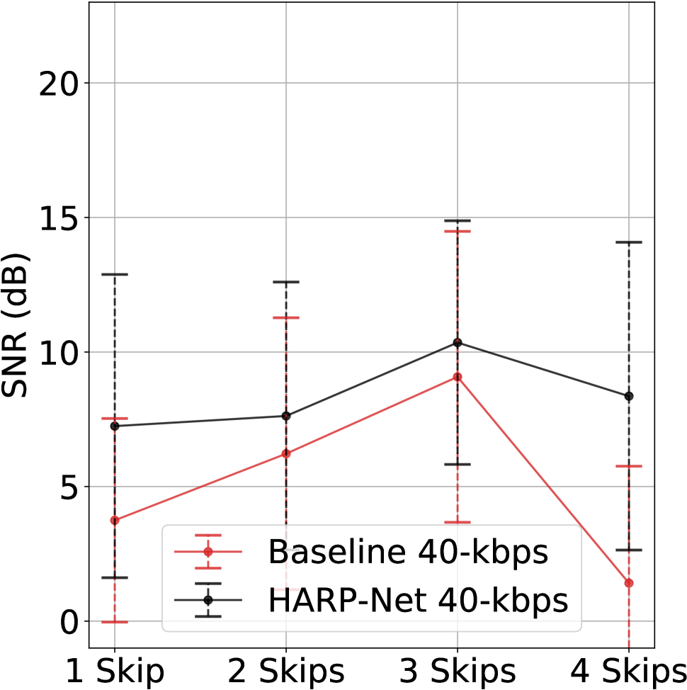
(a) 40kbps

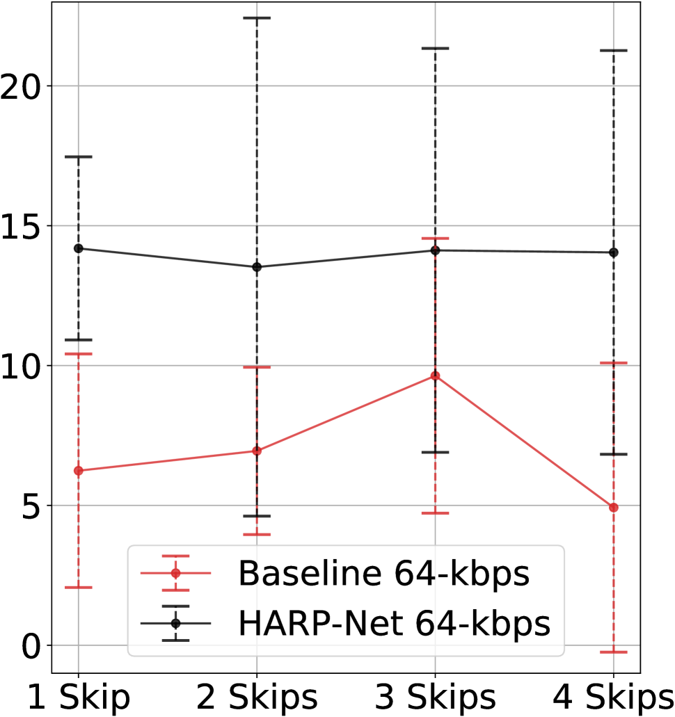
(b) 64kbps

Figure 2: SNR results of HARP-Net models and their associated baselines. Note that the baselines do not have skip connections.

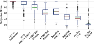
Figure 3: MUSHRA evaluation results in boxplots; green dotted line depicts the mean while the red line represent the median.

Fig.2 shows the average test SNR scores. We found that the low bitrate systems are affected more by the architectural choice, so we choose HARP-Net 3 and Baseline 3 as the best models used for subjective tests. However, note that this choice is not completely reliable due to its objective nature. Meanwhile, HARP-Net systems are not affected too much by the number of skip connections in the high bitrate cases, so we choose HARP-Net 1. It is noticeable that the baselines’ performance does not improve much by increasing target bitrate. We choose Baseline 3 as the best model for 64kbps.

The subjective test follows ITU’s MUSHRA guideline [21]. A session consists of nine different trials, each of which includes song segments from the same test set we have set aside. We select these segments in a manner that the subjects are exposed to a wide variety of music genres, consequently covering a range of auditory qualities and aspects. Each trial includes a hidden reference along with two low-pass filtered anchors per the MUSHRA specification. The systems in comparison are two HARP-Net models in two bitrates and their corresponding baselines that are chosen based on the SNR scores. Finally, we also include the MP3 decoded signals using Adobe Audition ®(licensed from Fraunhofer IIS and Thomson) at 64kbps. Note, however, that the MP3 signals are downsampled to $32$kHz by default. We recruit 12 audio experts, but excluded one of them who did not meet the post-screening guideline [21].

In Fig.3, both of our proposed systems (HARP-Net 64kbps and 40kbps) outperform their baseline counterparts. Moreover, we observe that the 40kbps HARP-Net performs within the same score span as the 64kbps baseline. Lastly, we note that HARP-Net 64kbps results lay close to the MP3 performance. Given that our LPC part is not optimal and our models cover wider bandwidth, i.e., 44.1kHz instead of 32kHz, the HARP-Net results are promising.

5 Conclusions

In this work we proposed a novel, lightweight, neural audio coding system, HARP-Net. It is defined as a mirrored AE with interconnected encoder-decoder layers via additional skip AEs. We found that those additional skip AEs create information paths that circumvent the lossy bottleneck quantization process, thus improving the total AE reconstruction performance. The skip AEs are carefully designed to work as a mini codec not to consume too much bitrates. Listening tests verified that the subjects prefer HARP-Net to the basic AE-based codecs. In the future, we will improve the LPC module’s bitrate, which can go down to 2.4kbps, and incorporate perceptually-motivated losses as proposed in [12]. Source codes and sound examples are available at https://saige.sice.indiana.edu/research-projects/harp-net.

References

- [1] ISO/IEC DIS 23003-3, “Information technology – MPEG audio technologies – part 3: Unified speech and audio coding,” 2011.
- [2] ISO/IEC 14496-3:2009/PDAM 3, “Transport of unified speech and audio coding (USAC),” 2011.
- [3] B. Bessette, R. Salami, R. Lefebvre, M. Jelinek, J. Rotola-Pukkila, J. Vainio, H. Mikkola, and K. Jarvinen, “The adaptive multirate wideband speech codec (AMR-WB),” IEEE Transactions on Speech and Audio Processing, vol. 10, no. 8, pp. 620–636, 2002.
- [4] J. M. Valin, K. Vos, and T. Terriberry, “Definition of the opus audio codec,” IETF, September, 2012.
- [5] S. Kankanahalli, “End-to-end optimized speech coding with deep neural networks,” in Proceedings of the IEEE International Conference on Acoustics, Speech, and Signal Processing (ICASSP), 2018.
- [6] K. Zhen, M. S. Lee, J. Sung, S. Beack, and M. Kim, “Efficient and scalable neural residual waveform coding with collaborative quantization,” in Proceedings of the IEEE International Conference on Acoustics, Speech, and Signal Processing (ICASSP), 2020.
- [7] A. van den Oord, S. Dieleman, H. Zen, K. Simonyan, O. Vinyals, A. Graves, N. Kalchbrenner, A. Senior, and K. Kavukcuoglu, “Wavenet: A generative model for raw audio,” arXiv preprint arXiv:1609.03499, 2016.
- [8] W. B. Kleijn, F. S. C. Lim, A. Luebs, J. Skoglund, F. Stimberg, Q. Wang, and T. C. Walters, “WaveNet based low rate speech coding,” in Proceedings of the IEEE International Conference on Acoustics, Speech, and Signal Processing (ICASSP), 2018, pp. 676–680.
- [9] Y. L. C. Garbacea, A. van den Oord, “Low bit-rate speech coding with VQ-VAE and a wavenet decoder,” in Proceedings of the IEEE International Conference on Acoustics, Speech, and Signal Processing (ICASSP), 2019.
- [10] J.-M. Valin and J. Skoglund, “LPCNet: Improving neural speech synthesis through linear prediction,” in Proceedings of the IEEE International Conference on Acoustics, Speech, and Signal Processing (ICASSP), 2019.
- [11] ——, “A real-time wideband neural vocoder at 1.6 kb/s using LPCNet,” in Proceedings of the Annual Conference of the International Speech Communication Association (Interspeech), 2019.
- [12] K. Zhen, M. S. Lee, J. Sung, S. Beack, and M. Kim, “Psychoacoustic calibration of loss functions for efficient end-to-end neural audio coding,” IEEE Signal Processing Letters, vol. 27, pp. 2159–2163, 2020.
- [13] K. Zhen, J. Sung, M. S. Lee, S. Beack, and M. Kim, “Cascaded cross-module residual learning towards lightweight end-to-end speech coding,” in Proceedings of the Annual Conference of the International Speech Communication Association (Interspeech), 2019.
- [14] O. Ronneberger, P. Fischer, and T. Brox, “U-net: Convolutional networks for biomedical image segmentation,” in International Conference on Medical image computing and computer-assisted intervention. Springer, 2015, pp. 234–241.
- [15] D. Stoller, S. Ewert, and S. Dixon, “Wave-u-net: A multi-scale neural network for end-to-end audio source separation,” in Proceedings of the International Society for Music Information Retrieval Conference (ISMIR), 2018.
- [16] G. E. Hinton and R. R. Salakhutdinov, “Reducing the dimensionality of data with neural networks,” Science, vol. 313, no. 5786, pp. 504–507, 2006.
- [17] E. Agustsson, F. Mentzer, M. Tschannen, L. Cavigelli, R. Timofte, L. Benini, and L. V. Gool, “Soft-to-hard vector quantization for end-to-end learning compressible representations,” in Advances in Neural Information Processing Systems (NIPS), 2017, pp. 1141–1151.
- [18] A. Jansson, E. Humphrey, N. Montecchio, R. Bittner, A. Kumar, and T. Weyde, “Singing voice separation with deep u-net convolutional networks,” in Proceedings of the International Society for Music Information Retrieval Conference (ISMIR), October 2017.
- [19] W. Shi, J. Caballero, F. Huszár, J. Totz, A. P. Aitken, R. Bishop, D. Rueckert, and Z. Wang, “Real-time single image and video super-resolution using an efficient sub-pixel convolutional neural network,” in Proceedings of the IEEE International Conference on Computer Vision and Pattern Recognition (CVPR), 2016, pp. 1874–1883.
- [20] V. Emiya, E. Vincent, N. Harlander, and V. Hohmann, “Subjective and objective quality assessment of audio source separation,” IEEE Transactions on Audio, Speech, and Language Processing, vol. 19, no. 7, pp. 2046–2057, 2011.
- [21] ITU-R Recommendation BS 1534-1, “Method for the subjective assessment of intermediate quality levels of coding systems (MUSHRA),” 2003.