Query2Label: A Simple Transformer Way to Multi-Label Classification

Abstract

This paper presents a simple and effective approach to solving the multi-label classification problem. The proposed approach leverages Transformer decoders to query the existence of a class label. The use of Transformer is rooted in the need of extracting local discriminative features adaptively for different labels, which is a strongly desired property due to the existence of multiple objects in one image. The built-in cross-attention module in the Transformer decoder offers an effective way to use label embeddings as queries to probe and pool class-related features from a feature map computed by a vision backbone for subsequent binary classifications. Compared with prior works, the new framework is simple, using standard Transformers and vision backbones, and effective, consistently outperforming all previous works on five multi-label classification data sets, including MS-COCO, PASCAL VOC, NUS-WIDE, and Visual Genome. Particularly, we establish $91.3\%$ mAP on MS-COCO. We hope its compact structure, simple implementation, and superior performance serve as a strong baseline for multi-label classification tasks and future studies. The code will be available soon at https://github.com/SlongLiu/query2labels.

1 Introduction

Multi-label image classification aims to gain a comprehensive understanding of objects and concepts in an image which has wide applications in realistic scenarios including image search, personal photo organization, digital asset management, medical image recognition [21], and scene understanding [41]. Compared with single label classification, multi-label classification requires special attention on two problems: 1) how to handle the label imbalance problem, and 2) how to extract features from region of interests. The former problem is because of the one-vs-all strategy, i.e., it usually trains a batch of separate binary classifiers with each designed for recognizing a particular class, which may lead to severely imbalanced numbers of positive and negative samples especially when the number of classes is large . The latter problem is because of the distributed objects, i.e., an image often has multiple objects at different locations – a globally pooled feature as normally used in single label classification may dilute the features and make it hard to identify small objects.

It has witnessed significant attempts to solve the aforementioned issues. To balance positive and negative samples, many loss functions have been developed, such as focal loss [34], distribution-balanced loss [50], and asymmetric loss [1]. Some works have tried to address the second problem by utilizing spatial transformer network [47], adopting a global-to-local strategy [19], or using semantic label embeddings learned from label graph to discover the locations of discriminative features [53]. Compared with the first issue, solutions for the second problem are relatively less mature, requiring either specially designed network architectures or additional dependencies on label correlation.

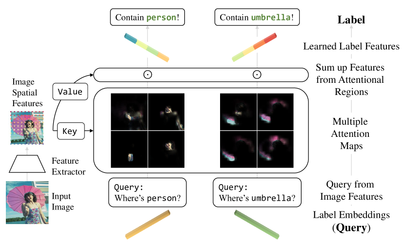
Figure 1: Illustration of Query2Label. Using cross attention for adaptively feature pooling through focusing on different parts (best view in colors).

Motivated by the success of Transformer used in computer vision tasks [3, 17], we present in this paper a simple yet effective solution using Transformer decoder to query the existence of a class label. We show that, without bells and whistles, the proposed solution leads to new state-of-the-art results and establishes strong baselines for its simple implementation and superior performance. We name the proposed solution as Query2Label and illustrate it in Fig. 1. As shown in the figure, we use learnable label embeddings as queries to probe and pool class-related features via the cross-attention module in Transformer encoders. The pooled features are adaptive and more discriminative, leading to a superior multi-label classification performance.

The use of Transformer for solving multi-label classification is rooted in the need of extracting local discriminative features adaptively for different labels, which is a strongly desired property due to the existence of multiple objects in one image. While previous works [56, 1] show that it is possible to use the globally average-pooled feature from the last layer of a convolutional neural network (CNN) for its simplicity in implementation, we argue that this will lead to inferior performance due to its discard of rich information in the convolutional feature map. The built-in cross-attention mechanism, which is called encoder-decoder attention in  [45], makes Transformer decoder a perfect choice for adaptively extracting desired features. By treating each label class as a query in a Transformer decoder, we can perform cross-attention to pool related features for the subsequent binary classification. The most related work to this idea is developed by You et al. [53], which, however, computes attention using cosine similarity with negative value clipping and uses the same feature for both key and value, greatly limiting its capability of learning locally discriminative features.

Another advantage of Transformer is its multi-head attention mechanism, which can extract features from different parts or different views of an object class and thus is more capable of recognizing objects with occlusions and viewpoint changes. By contrast, the cross-modal attention in  [53] is merely a single-head attention, which is incapable of extracting features by parts or views.

In this work, we develop a simple two-stage framework called Query2Label for multi-label classification by leveraging multi-layer Transformer decoders. In the first stage, we use an image classification backbone to extract image features. The backbone could be either conventional CNN models such as ResNet [25] or recently developed Vision Transformer models [17]. In the second stage, multiple Transformer decoder layers are leveraged, using label embeddings as queries to check the existence of each label by performing multi-head cross-attention to pool object features adaptively for subsequent binary classification to predict the existence of the corresponding label. Unlike  [53] in which the label embeddings are learned separately to take into account label correlations, we learn the label embeddings end-to-end to maximize the model potential and avoid the risk of introducing spurious correlations. The idea of using learnable label embeddings is inspired by DETR [3]. But the queries in DETR are class agnostic, whereas in our work each query (or label embedding) uniquely corresponds to one label class, making it more effective to extract class-related features. For this reason, in this paper, we will use label embedding and query interchangeably.

To handle the label imbalance problem, we adopt a simplified asymmetric loss [1] by using different $\gamma$ values to weight positive and negative samples differently in focal loss. We found that this simple asymmetric loss works sufficiently well with this Transformer-based framework and leads to new state-of-the-art results on several multi-label benchmark data sets, including MS-COCO, PASCAL VOC, NUS-WIDE, and Visual Genome.

Our contribution can be summarized as follows:

1. We develop a simple Transformer-based two-stage framework Query2Label for multi-label classification, leading to an effective way to query the existence of a class label. To our best knowledge, this is the first time that the Transformer decoder architecture is used in classification.

2. We show that, the built-in cross-attention module in Transformer decoders can adaptively extract object features and the multi-head attention further helps to decouple object representations into multiple parts or views, resulting in both improved classification performance and better interpretability.

3. We verify the effectiveness of the proposed method with comprehensive experiments on several widely used data sets: MS-COCO, PASCAL VOC, NUSWIDE, and Visual Genome, and establish new state-of-the-art results on all these data sets.

2 Related Work

2.1 Multi-Label Classification

Multi-label classification task has attracted an increasing interest recently. The proposed methods can be categorized into three main directions as follows:

Improving loss functions. As shown in Sec. 1, one of the key concerns in multi-label classification is the imbalance of samples due to the use of one-vs-rest binary classifier for each category. Wu et al. [50] proposed a distribution-balanced loss to tackle the long-tailed problem by re-balancing weights and mitigating the over-suppression of negative labels. Ben-Baruch et al. [1] proposed an asymmetric loss, which uses different $\gamma$ values to weight positive and negative samples in focal loss [34], and discarding easy negative samples by shifting the prediction probability. In our study, we adopt a simplified asymmetric loss which uses different $\gamma$ values for positive and negative samples without prediction probability shift.

Modeling label correlations. For its nature of multi-labels on one image, the co-occurrence of concepts in a large-scale data set could be mined as prior knowledge for subsequent classification. Chen et al. [7] proposed to learn category-correlated feature vectors by constructing a graph based on the statistical label co-occurrence and explored their interactions by performing neural graph propagation. Chen et al. [8] constructed a similar graph but based on class-aware maps, which is calculated by image level feature and classification weights, and constrained the graph by label co-occurrence. Rather than using static graph, Ye et al. [52] updated static graph to dynamic graph by using a dynamic graph convolutional network(GCN) module for robust representations. While modeling label correlations can introduce additional gains in multi-label classification, it is also arguable that it may learn spurious correlations when the label statistics are insufficient. In our study, we directly learn label embeddings from data and encourage the network to focus on regions of interest to learn better feature representations and capture label relationships implicitly without graph networks.

Locating regions of interest. As an image normally has multiple objects, how to locate areas of interest becomes a concern in multi-label classification. Early methods [48, 51] found proposals first and treated them as single-label classification. Wang et al. [47] proposed to locate attentional regions corresponding to semantic labels by using a spatial transformer layer [27] and predicted their scores with a Long Short-Term Memory (LSTM) sub-network [26]. Gao et al. [19] proposed a global-to-local discovery method to find proper regions with objects. All of these methods tried to find local regions to focus, but the discovered bounding boxes were coarse and often contained background information as well. You et al. [53] computed cosine similarities between a label embedding and the feature map to derive an attention map after clipping negative values for class feature learning, which is a step forward. However, the cosine similarity with negative value clipping is likely to lead to a smoother and none spike attention, making it less effective in extracting desired local features (because it will cover larger areas than needed, see the visualized attention in Fig. 4 in [53]). By contrast, we adopt the built-in cross-attention in Transformer as spatial feature selector to extract desired features, which is both simple and effective, thanks to the modularized design of Transformer and its readily available implementations in modern deep learning frameworks.

2.2 Transformer in Vision Tasks

Transformer [45] was first proposed to model long-range dependencies in sequence learning problems, and has been widely used in natural language processing tasks [15, 32, 13, 2, 31, 55]. Recently, Transformer-based models have also been developed for many vision tasks  [17, 54, 44, 3, 57, 4, 22, 23] and shown great potentials. Chen et al. [5] trained a sequence Transformer, named iGPT, to predict pixels auto-regressively. Dosovitskiy et al. [17] proposed Vision Transformers (ViT), in which they split an image to multiple patches and feed them into a stacked Transformer architecture for classification. Carion et al. [3] designed an end-to-end object detection framework named DETR with transformer. Yuan et al. [54] proposed Tokens-To-Token Vision Transformer (T2T-ViT) to address the patch tokenization problem. Srinivas et al. [44] replaced convolutional layers in last few ResNet Bottleneck [25] with Multi-Head Self-Attention and capture better global dependencies. More progress of applying Transformer in computer vision can be referred to [24] and [28].

Our approach also uses Transformers, but we leverage the built-in cross-attention in the Transformer decoder to locate object features for each label, which is largely different from most existing works  [17, 54, 44, 10] using the self-attention mechanism in Transformer encoders to improve feature representation. Our work is inspired by DETR [3], but different in that the queries in DETR are class-agnostic and do not have clear semantics, whereas each query in our work uniquely corresponds to a semantic label.

3 Method

Query2Label is a two-stage framework for multi-label classification, which uses Transformer decoders to extract features with multi-head attentions focusing on different parts or views of an object category and learn label embeddings from data automatically. In this section, we will present our framework first (Sec. 3.1), followed with a brief description to the loss function used (Sec. 3.2).

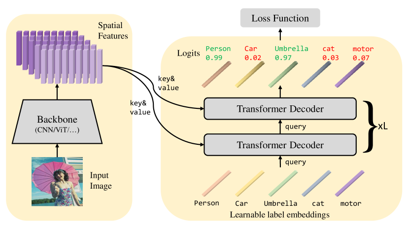
Figure 2: The framework of our proposed Query2Label (Q2L). After extracting spatial features of an input image, each label embedding is sent to Transformer decoders to query (by comparing the label embedding with features at each spatial location to generate attention maps) and pool the desired feature adaptively (by linearly combining the spatial features based on the attention maps). The pooled feature is then used to predict the existence of the queried label.

3.1 Framework

Given an input image $x$, among a set of categories of interest, multi-label classification is to predict whether each category is present. A category could be either an object class (e.g. person, dog, table, etc.) or a scene category (grass, sky, etc). Assume there are $K$ categories in total and we denote the corresponding label of $x$ as $y=[y_{1},...,y_{K}]$, where $y_{k}\in\{0,1\},k=1,...,K$, is a discrete binary indicator. $y_{k}=1$ if image $x$ has the $k$-th category label, otherwise $y_{k}=0$. Using $x$ as input, our model predicts the probabilities of the presence of each category, $p=[p_{1},...,p_{K}]$, where $y_{k}\in[0,1],k=1,...,K$.

Fig. 2 illustrates the framework of the proposed Query2Label (Q2L). For an input image, it firstly feeds it into a backbone in the first stage to extract spatial features. The second stage is composed of two modules: a multi-layer Transformer decoder block for query updating and adaptive feature pooling, and a linear projection layer for computing prediction logits for each category. Note that our method is backbone-agnostic. That is, the second stage could be attached to any feature extractor. In this work, we mainly use convolutional neural networks as the feature extraction backbone, but Transformer-based networks such as ViT [17] can also be used.

Feature extracting. Given an image $x\in\mathbb{R}^{H_{0}\times W_{0}\times 3}$ as input, we extract its spatial features $\mathcal{F}_{0}\in\mathbb{R}^{H\times W\times d_{0}}$ using the backbone, where $H_{0}\times W_{0}$, $H\times W$ represent the height and weight of the input image and the feature map respectively, and $d_{0}$ denotes the dimension of features. After that, we add a linear projection layer to project the features from dimension $d_{0}$ to $d$ to match with the desired query dimension in the second stage and reshape the projected features to be $\mathcal{F}\in\mathbb{R}^{HW\times d}$.

Query updating. After obtaining the spatial features of the input image in the first stage, we use label embeddings as queries $\mathcal{Q}_{0}\in\mathbb{R}^{K\times d}$ and perform cross-attention to pool category-related features from the spatial features using multi-layer Transformer decoders, where $K$ is the number of categories. We use the standard Transformer architecture, which has a self-attention module, a cross-attention module, and a position-wise feed-forward network(FFN). Each Transformer decoder layer $i$ updates the queries $\mathcal{Q}_{i-1}$ from the output of its previous layer as follows:

self-attn: $$\mathcal{Q}_{i}^{(1)}=\text{MultiHead}(\widetilde{\mathcal{Q}}_{i-1},\widetilde{\mathcal{Q}}_{i-1},\mathcal{Q}_{i-1}),$$ (1)

cross-attn: $$\mathcal{Q}_{i}^{(2)}=\text{MultiHead}(\widetilde{\mathcal{Q}}_{i}^{(1)},\widetilde{\mathcal{F}},{\mathcal{F}}),$$ (2)

FFN: $$\mathcal{Q}_{i}=\text{FFN}(\mathcal{Q}_{i}^{(2)}),$$ (3)

where the tilde means the original vectors modified by adding position encodings, $\mathcal{Q}_{i}^{(1)}$ and $\mathcal{Q}_{i}^{(2)}$ are two intermediate variables. Both the MultiHead(query, key, value) and $\text{FFN(}x\text{)}$ functions are the same as defined in the standard Transformer decoder [45] and we omit their parameters for simplicity. As we do not need to perform auto-regressive prediction, we do not use attention masks. Thus the $M$ categories can be decoded in parallel in each layer.

Both the self-attention and cross-attention modules are implemented using the same MultiHead function. The only difference is where key and value are from. In the self-attention module, query, key and value are all from label embeddings, whereas in the cross-attention module, key and value turn into the spatial features. The process of cross-attention can be described more intuitively: each label embedding $\mathcal{Q}_{{i-1},k}\in\mathbb{R}^{d},k=1,...,K$ checks the spatial features $\widetilde{\mathcal{F}}$ where to attend and selects features of interest to combine. After that, each label embedding obtains a better category-related feature and updates itself. As a result, the label embeddings $\mathcal{Q}_{0}$ will be updated layer by layer and progressively injected with contextualized information from the input image via cross-attention.

Inspired by DETR, we treat the label embeddings $\mathcal{Q}_{0}$ as learnable parameters. In this way, the embeddings can be learned end to end from data and model label correlations implicitly. The difference between our approach and DETR is that our queries are class-specific and have clear semantic meanings, whereas the queries in DETR are class-agnostic and it is hard to predict which query will detect which category of objects.

Feature Projection. Assuming that we have $L$ layers in total, we will get the queried feature vectors $\mathcal{Q}_{L}\in\mathbb{R}^{K\times d}$ for $K$ categories at the last layer. To perform multi-label classification, we treat each label prediction as a binary classification task and project the feature of each class $\mathcal{Q}_{L,k}\in\mathbb{R}^{d}$ to a logit value using a linear projection layer followed with a sigmoid function:

$$p_{k}=\text{Sigmoid}\left(W_{k}^{T}\mathcal{Q}_{L,k}+b_{k}\right),$$ (4)

where $W_{k}\in\mathbb{R}^{d}$, $W=[W_{1},...,W_{K}]^{T}\in\mathbb{R}^{K\times d}$, and $b_{k}\in\mathbb{R}$, $b=[b_{1},...,b_{K}]^{T}\in\mathbb{R}^{K}$ are parameters in the linear layer, and $p=[p_{1},...,p_{K}]^{T}\in\mathbb{R}^{K}$ are the predicted probabilities for each category. Note that $p$ is a function which maps an input image $x$ to category prediction probabilities. $x$ is omitted for notation simplicity.

3.2 Loss Function

Thanks to the built-in cross-attention mechanism in Transformer decoders, our framework does not require a new loss function. Both the binary cross entropy loss and focal loss [34] work well with our framework. To more effectively address the sample imbalance problem, we adopt a simplified asymmetric loss [1], which is a variant of focal loss with different $\gamma$ values for positive and negative values. In our experiments, we found it works the best.

Given an input images $x$, we can predict its category probabilities $p=[p_{1},...,p_{K}]^{T}\in\mathbb{R}^{K}$ using our framework. Then we leverage the following asymmetric focal loss to calculate the loss for each training sample $x$:

$$\mathcal{L}=\frac{1}{K}\sum_{k=1}^{K}\begin{cases}(1-p_{k})^{\gamma+}\log(p_{k}),&y_{k}=1,\\ (p_{k})^{\gamma-}\log(1-p_{k}),&y_{k}=0,\\ \end{cases}$$ (5)

where $y_{k}$ is a binary label to indicate if image $x$ has label $k$. The total loss is computed by averaging this loss over all samples in the training data set $\mathcal{D}$. And the optimization is performed using stochastic gradient descent. By default, we set $\gamma+=0$ and $\gamma-=1$ in our experiments.

4 Experiments

To evaluate the proposed approach, we conduct experiments on several data sets, including MS-COCO [35], PASCAL VOC [18], NUS-WIDE [11], and Visual Genome [30]. Following previous works, we adopt the average precision (AP) on each category and mean average precision (mAP) over all categories for evaluation. To better demonstrate the performance of models, we also present the overall precision (OP), recall (OR), F1-measure (OF1) and per-category precision (CP), recall (CR), F1-measure (CF1) for further comparison. See appendix for a more formal definition of these metrics.

4.1 Implementation Details

Unless otherwise stated, we will use the settings described below for all experiments. Following ASL [1], We adopt TResNetL [40] as our backbone, as it performs better than the standard ResNet101 [25] for this task under similar efficiency constraints on GPU. We resize all images to $H_{0}\times W_{0}=448\times 448$ as the input resolution and the size of the output feature from TResNetL is $H\times W\times d_{0}=14\times 14\times 2432$. We set $d=d_{0}=2432$ in our experiments, hence the size of the final output feature in the first stage is $14\times 14\times 2432$. The extracted features are fed into the second stage module after adding position encodings and reshaping. For the second stage, we utilize one Transformer encoder layer and two Transformer decoder layers for label feature updating. After the last Transformer decoder, we add a linear projection layer to compute logit predictions for all categories.

Note that the Transformer encoder is mainly used to further help fuse global context for better feature representation, but it can be removed for more efficient computation. In our experiments, our model works well even with only one Transformer decoder layer. See more ablations in Sec. 4.3.

We leverage the ImageNet [14] pre-trained model as our backbone, and update the whole model on the target multi-label classification data set. We trained the model for 80 epochs using the Adam [29] optimizer, with True-weight-decay [38] of $1e-2$, $(\beta_{1},\beta_{2})=(0.9,0.9999)$, and a learning rate of $1\times 10^{-4}$. More implementation and training details are available in the supplementary materials.

4.2 Comparison with State-of-the-art Methods

4.2.1 Performance on MS-COCO

MS-COCO [35] is a large-scale data set constructed for object detection and segmentation firstly and has been widely used for evaluating multi-label image classification recently. It contains $122,218$ images and covers $80$ common objects, with an average of $2.9$ labels per image. Notice that the mAP scores for MS-COCO are highly influenced by the input resolution. Thus we divide the results into two groups: medium resolution ($H,W\leq 600$) and high resolution($H,W>600$) and report them separately.

For the medium resolution, we adopt our standard setting and report the comparison between our method and other state-of-the-art methods in Table 1. All the methods are evaluated in the resolution of $448\times 448$, except for SSGRL in $576\times 576$ and ADD-GCN in $512\times 512$. Our proposed method outperforms all the previous methods in terms of mAP, OF1, and CF1, which are the most important metrics, as other metrics can be affected by the chosen threshold largely. In particular, our Q2L respectively outperforms ADD-GCN by $2.0\%$, SSGRL by $3.4\%$, and ASL by $0.6\%$. That demonstrates the superiority of our approach.

Method	Backbone	Resolution	mAP	All						Top 3
				CP	CR	CF1	OP	OR	OF1	CP	CR	CF1	OP	OR	OF1
SRN [56]	ResNet101	224$\times$224	77.1	81.6	65.4	71.2	82.7	69.9	75.8	85.2	58.8	67.4	87.4	62.5	72.9
ResNet-101 [25]	ResNet101	224$\times$224	78.3	80.2	66.7	72.8	83.9	70.8	76.8	84.1	59.4	69.7	89.1	62.8	73.6
CADM [8]	ResNet101	448$\times$448	82.3	82.5	72.2	77.0	84.0	75.6	79.6	87.1	63.6	73.5	89.4	66.0	76.0
ML-GCN [9]	ResNet101	448$\times$448	83.0	85.1	72.0	78.0	85.8	75.4	80.3	87.2	64.6	74.2	89.1	66.7	76.3
KSSNet [36]	ResNet101	448$\times$448	83.7	84.6	73.2	77.2	87.8	76.2	81.5	-	-	-	-	-	-
MS-CMA [53]	ResNet101	448$\times$448	83.8	82.9	74.4	78.4	84.4	77.9	81.0	86.7	64.9	74.3	90.9	67.2	77.2
MCAR [20]	ResNet101	448$\times$448	83.8	85.0	72.1	78.0	88.0	73.9	80.3	88.1	65.5	75.1	91.0	66.3	76.7
SSGRL [7]	ResNet101	576$\times$576	83.8	89.9	68.5	76.8	91.3	70.8	79.7	91.9	62.5	72.7	93.8	64.1	76.2
C-Trans [33]	ResNet101	576$\times$576	85.1	86.3	74.3	79.9	87.7	76.5	81.7	90.1	65.7	76.0	92.1	71.4	77.6
ADD-GCN [52]	ResNet101	576$\times$576	85.2	84.7	75.9	80.1	84.9	79.4	82.0	88.8	66.2	75.8	90.3	68.5	77.9
Q2L-R101(Ours)	ResNet101	448$\times$448	84.9	84.8	74.5	79.3	86.6	76.9	81.5	78.0	69.1	73.3	80.7	70.8	75.4
Q2L-R101(Ours)	ResNet101	576$\times$576	86.5	85.8	76.7	81.0	87.0	78.9	82.8	90.4	66.3	76.5	92.4	67.9	78.3
ASL [1]	TResNetL	448$\times$448	86.6	87.2	76.4	81.4	88.2	79.2	81.8	91.8	63.4	75.1	92.9	66.4	77.4
TResNetL [39]	TResNetL(22k)	448$\times$448	88.4	-	-	-	-	-	-	-	-	-	-	-	-
Q2L-TResL(Ours)	TResNetL	448$\times$448	87.3	87.6	76.5	81.6	88.4	78.5	83.1	91.9	66.2	77.0	93.5	67.6	78.5
Q2L-TResL(Ours)	TResNetL(22k)	448$\times$448	89.2	86.3	81.4	83.8	86.5	83.3	84.9	91.6	69.4	79.0	92.9	70.5	80.2
MlTr-l [10]	MLTr-l(22k)	384$\times$384	88.5	86.0	81.4	83.3	86.5	83.4	84.9	-	-	-	-	-	-
Swin-L [37]	Swin-L(22k)	384$\times$384	89.6	89.9	80.2	84.8	90.4	82.1	86.1	93.6	69.9	80.0	94.3	71.1	81.1
CvT-w24 [49]	CvT-w24(22k)	384$\times$384	90.5	89.4	81.7	85.4	89.6	83.8	86.6	93.3	70.5	80.3	94.1	71.5	81.3
Q2L-SwinL(Ours)	Swin-L(22k)	384$\times$384	90.5	89.4	81.7	85.4	89.8	83.2	86.4	93.9	70.4	80.5	94.8	71.0	81.2
Q2L-CvT(Ours)	CvT-w24(22k)	384$\times$384	91.3	88.8	83.2	85.9	89.2	84.6	86.8	92.8	71.6	80.8	93.9	72.1	81.6

Table 1: Comparison of our method with known state-of-the-art models on MS-COCO at medium input resolution. The backbones noted with 22k are pretrained on the ImageNet-22k dataset. Among them, mAP, OF1, and CF1 are the primary metrics (shaded in the table) as the others may be affected by the chosen threshold largely. All metrics are in %.

For high resolution($640\times 640$) experiments, we adopt TResNetXL [40] as the backbone and remove the self-attention module in Transformer decoders for better training and inference efficiency. The results are shown in Table 2. Our method outperforms the best result in the literature and establishes a new state of the art.

Method	Architecture	Input Resolution	mAP
ASL [1]	TResNetXL	640$\times$640	88.4
TResNet [39]	TResNetL(22k)	640$\times$640	89.8
Q2L-TResXL	TResNetXL	640$\times$640	89.0
Q2L-TResL	TResNetL(22k)	640$\times$640	90.3

Table 2: Comparison of our method with ASL on MS-COCO for high input resolution of $640\times 640$. All metrics are in %.

4.2.2 Performance on PASCAL VOC

PASCAL VOC 2007 and 2012 [18] are two frequently used data sets for multi-label classification. Each image in VOC contains one or multiple labels, corresponding to $20$ object categories. In order to fairly compare with other methods, we follow the common setting to train our model on the train-val set and then evaluate its performance on the test set. Following previous works, we also pre-train the model on COCO for better performance.

Results on VOC 07. VOC 2007 contains $5,011$ images as the train-val set, and $4,952$ images as the test set. Results on VOC 07 are shown in Table 3. We can see that our method achieves the best mAP performance among all methods. We also observe the small margin between our results and ADD-GCN [52]. In addition to the difference in input image resolution (ours $448\times 448$ and ADD-GCN’s $512\times 512$), the small increase may indicate the limited data of VOC 07 and its saturated metric. Nevertheless, there might be some other factors that influence the results, as we outperform previous works on VOC 12 with a larger margin as shown in Table 4, whose results are reported by the evaluation server. We report results with ImageNet-1K pretrained backbone only in the main text for a fair comparison, and results with advanced backbones could be found in the appendix.

Results on VOC 12. VOC 2012 consists of $11,540$ images as the train-val set and $10,991$ images as the test set. Results on VOC 12 are shown in Table 4. As all the results are reported by its evaluation server, it is a much fairer comparison than a local test. Our method outperforms all other methods on all metrics with a large margin.

Methods	aero	bike	bird	boat	bottle	bus	car	cat	chair	cow	table	dog	horse	mbike	person	plant	sheep	sofa	train	tv	mAP
CNN-RNN [46]	96.7	83.1	94.2	92.8	61.2	82.1	89.1	94.2	64.2	83.6	70.0	92.4	91.7	84.2	93.7	59.8	93.2	75.3	99.7	78.6	84.0
VGG+SVM [42]	98.9	95.0	96.8	95.4	69.7	90.4	93.5	96.0	74.2	86.6	87.8	96.0	96.3	93.1	97.2	70.0	92.1	80.3	98.1	87.0	89.7
Fev+Lv [51]	97.9	97.0	96.6	94.6	73.6	93.9	96.5	95.5	73.7	90.3	82.8	95.4	97.7	95.9	98.6	77.6	88.7	78.0	98.3	89.0	90.6
HCP [48]	98.6	97.1	98.0	95.6	75.3	94.7	95.8	97.3	73.1	90.2	80.0	97.3	96.1	94.9	96.3	78.3	94.7	76.2	97.9	91.5	90.9
RDAL [47]	98.6	97.4	96.3	96.2	75.2	92.4	96.5	97.1	76.5	92.0	87.7	96.8	97.5	93.8	98.5	81.6	93.7	82.8	98.6	89.3	91.9
RARL [6]	98.6	97.1	97.1	95.5	75.6	92.8	96.8	97.3	78.3	92.2	87.6	96.9	96.5	93.6	98.5	81.6	93.1	83.2	98.5	89.3	92.0
SSGRL [7] (576)	99.7	98.4	98.0	97.6	85.7	96.2	98.2	98.8	82.0	98.1	89.7	98.8	98.7	97.0	99.0	86.9	98.1	85.8	99.0	93.7	95.0
MCAR [19]	99.7	99.0	98.5	98.2	85.4	96.9	97.4	98.9	83.7	95.5	88.8	99.1	98.2	95.1	99.1	84.8	97.1	87.8	98.3	94.8	94.8
ASL(TResNetL) [1]	99.9	98.4	98.9	98.7	86.8	98.2	98.7	98.5	83.1	98.3	89.5	98.8	99.2	98.6	99.3	89.5	99.4	86.8	99.6	95.2	95.8
ADD-GCN [52] (576)	99.8	99.0	98.4	99.0	86.7	98.1	98.5	98.3	85.8	98.3	88.9	98.8	99.0	97.4	99.2	88.3	98.7	90.7	99.5	97.0	96.0
Q2L-TResL(Ours)	99.9	98.9	99.0	98.4	87.7	98.6	98.8	99.1	84.5	98.3	89.2	99.2	99.2	99.2	99.3	90.2	98.8	88.3	99.5	95.5	96.1

Table 3: Comparisons of our method with previous state-of-the-art methods on PASCAL VOC 2007, in terms of AP and mAP in $\%$. All results are reported at resolution $448\times 448$ except for the ADD-GCN and SSGRL, whose resolutions are noted in parentheses. Results with advanced backbones could be found in the appendix.

Methods	aero	bike	bird	boat	bottle	bus	car	cat	chair	cow	table	dog	horse	mbike	person	plant	sheep	sofa	train	tv	mAP
VGG+SVM [42]	99.0	89.1	96.0	94.1	74.1	92.2	85.3	97.9	79.9	92.0	83.7	97.5	96.5	94.7	97.1	63.7	93.6	75.2	97.4	87.8	89.3
Fev+Lv [51]	98.4	92.8	93.4	90.7	74.9	93.2	90.2	96.1	78.2	89.8	80.6	95.7	96.1	95.3	97.5	73.1	91.2	75.4	97.0	88.2	89.4
HCP [48]	99.1	92.8	97.4	94.4	79.9	93.6	89.8	98.2	78.2	94.9	79.8	97.8	97.0	93.8	96.4	74.3	94.7	71.9	96.7	88.6	90.5
MCAR [19]	99.6	97.1	98.3	96.6	87.0	95.5	94.4	98.8	87.0	96.9	85.0	98.7	98.3	97.3	99.0	83.8	96.8	83.7	98.3	93.5	94.3
SSGRL [7](576)	99.7	96.1	97.7	96.5	86.9	95.8	95.0	98.9	88.3	97.6	87.4	99.1	99.2	97.3	99.0	84.8	98.3	85.8	99.2	94.1	94.8
ADD-GCN [52](576)	99.8	97.1	98.6	96.8	89.4	97.1	96.5	99.3	89.0	97.7	87.5	99.2	99.1	97.7	99.1	86.3	98.8	87.0	99.3	95.4	95.5
Q2L-TResL(Ours)	99.9	98.2	99.3	98.1	90.4	97.7	97.4	99.4	92.7	98.7	89.9	99.4	99.5	99.0	99.4	88.4	98.8	89.3	99.6	96.8	96.6

Table 4: Comparisons of AP and mAP in $\%$ of our model and state-of-the-art methods on PASCAL VOC 2012. All results are reported at resolution 448$\times$448 except for the ADD-GCN and SSGRL, whose resolution is noted in parentheses. Different from VOC 07, results in VOC 12 are reported by the evaluation server.

4.2.3 Performance on NUS-WIDE

NUS-WIDE [11] is a real-world web image data set. It contains $269,648$ Flickr images and has been manually annotated with $81$ visual concepts. We follow the steps in [1] for evaluation, and compare the proposed method with previous state-of-the-art models in Table 5. As the resolutions of NUS-WIDE images are not high enough, we found the improvement of our method is not as significant as on MS-COCO and PASCAL VOC. But we still achieve a new state of the art on this data set.

Method	Backbone	mAP	CF1	OF1
MS-CMA [53]	ResNet101	61.4	60.5	73.8
SRN [56]	ResNet101	62.0	58.5	73.4
ICME [9]	ResNet101	62.8	60.7	74.1
Q2L-R101(Ours)	ResNet101	65.0	63.1	75.0
Baseline [40]	TresNetL	63.1	61.7	74.6
Focal loss [34]	TresNetL	64.0	62.9	74.7
ASL [1]	TresNetL	65.2	63.6	75.0
Q2L-TResL(Ours)	TresNetL	66.3	64.0	75.0
MlTr-l [10]	MlTr-l(22k)	66.3	65.0	75.8
Q2L-CvT(Ours)	CvT-w24(22k)	70.1	67.6	76.3

Table 5: Comparison of our methods to known state-of-the-art models on NUS-WIDE. The backbones noted with 22k are pretrained on the ImageNet-22k dataset. All metrics are in %.

4.2.4 Performance on Visual Genome

Visual Genome [30] is a data set that contains $108,249$ images and covers $80,138$ categories. As most categories contain very few samples, [7] select images with the most frequent $500$ categories, and split the data set into train and test sets. They call the new data set VG500. We follow their setting and compare our model with prior methods in Table 6. For a fair comparison, we set the resolution of input images to $512\times 512$, and evaluate our method using both the ResNet-101 [25] and TResNetL [40] backbones. Although the previous state-of-the-art model SSGRL [7] use larger image resolution ($576\times 576$) than ours ($512\times 512$), our method outperforms all previous works and achieves a new SOTA on VG500. As the number of categories in VG500 is much larger than other data sets, it becomes more challenging for a simple spatially average-pooled feature to recognize all of the objects. Hence the advantages of our method are more obvious. The results indicate the importance and effectiveness of spatially adaptive feature attention in multi-label classification, particularly when the number of categories is large.

Method	mAP
ResNet-101 [25]	30.9
ResNet-SRN [56]	33.5
SSGRL(ResNet101) [7]	36.6
C-Tran(ResNet101) [33]	38.4
Q2L-R101(Ours)	39.5
Q2L-TResL-22k(Ours)	42.5

Table 6: Comparison of our method with prior state-of-the-art methods on VG500. All metrics are in %. All results are reported at the input resolution of $576\times 576$.

4.3 Ablation Study

Results on objects of different sizes. To further test Q2L’s performance on objects of different sizes, we split the MS-COCO [35] test set into three subsets for small objects, medium objects, and large objects respectively. Following the common definition, objects occupying areas less than and equal to $32\times 32$ pixels are considered as “small objects”, less than and equal to $96\times 96$ pixels are marked as “medium objects”, and the others are “large objects”. We compare our Q2L with the baseline TResNetL model. The results are listed in Table 7. Our model outperforms baselines on all three categories, especially on medium objects. The larger improvement on medium objects demonstrates the superiority of the spatially adaptive feature pooling, which helps collect information that may be diluted by average pooling. For small objects, although our method has made a big step forward, it remains a challenging problem to be solved, requiring finer-grained details to be extracted from images.

Method	small	medium	large
Baseline(TResNetL) [40]	37.8	74.2	84.2
Ours(TResNetL+Q2L)	39.5	77.5	86.1

Table 7: Comparison of improvement on objects with different sizes.

4.4 Visualization of Attention Maps

To further demonstrate the effectiveness of cross-attention and adaptive pooling, we visualize some attention maps in Fig. 3. The attention map is analogous to the receptive field size in a raw image. We found that our model can locate the specified object approximately, especially on some small or medium objects. We also compare our Q2L model with baseline in Fig. 4. It validates the effectiveness of the spatial adaptive pooling built into Transformer decoders and shows great potential for providing better interpretability.

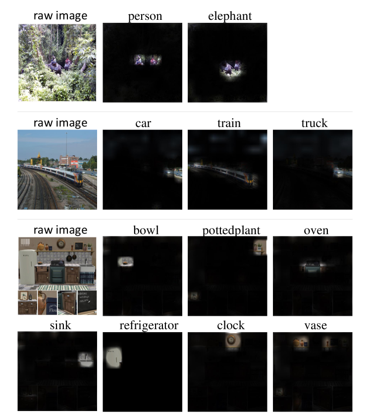
Figure 3: Visualization of cross-attention maps. We plot the mean of each head’s cross-attention maps, that represent similarities of a given query and extracted spatial features. Texts above images represent the ground truth labels (query) for the raw images. Best view in colors.

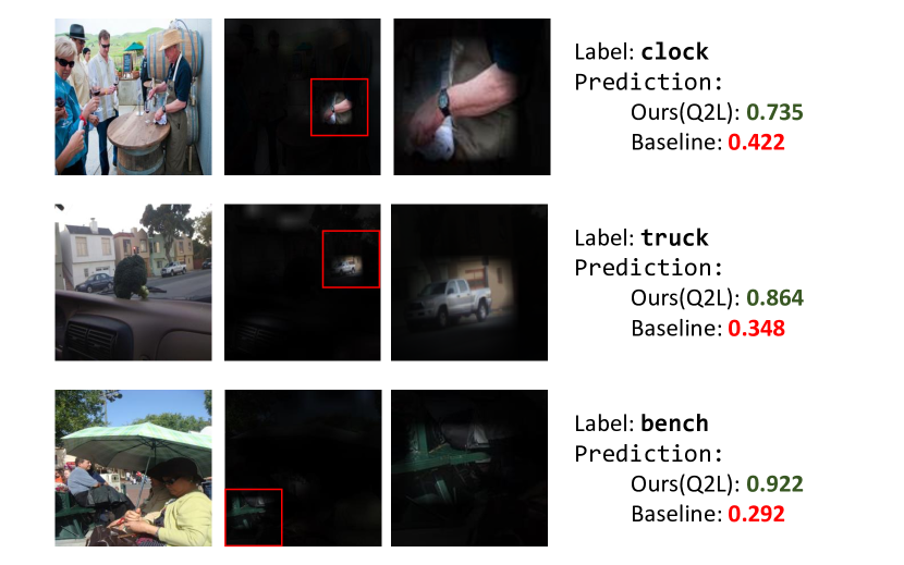
Figure 4: Image examples classified correctly by Q2L but wrongly by the baseline TResNetL. The middle two columns are the mean attention maps of Q2L and the enlarged maps on focused regions respectively. The small scale of objects makes it difficult for TResNetL to recognize. Best view in colors.

Beyond single attention maps, we are also interested in finding out the role of multi-head attention in this task. For a given target person, we plot individual attention maps in each head and the mean attention map in Fig. 5. We find that different heads are capable of focusing on different parts of targets. For person, head-1, head-3, and head-4 focus on the shoulder, neck, and head respectively. The attention maps of head-2 are less informative, as there is no clear focus, which may indicate that head-2 is not utilized as the other three heads already collect sufficient information for classification. Focusing on different parts makes the model more robust to occlusion and view changes, and provides better interpretability for the superiority of our model.

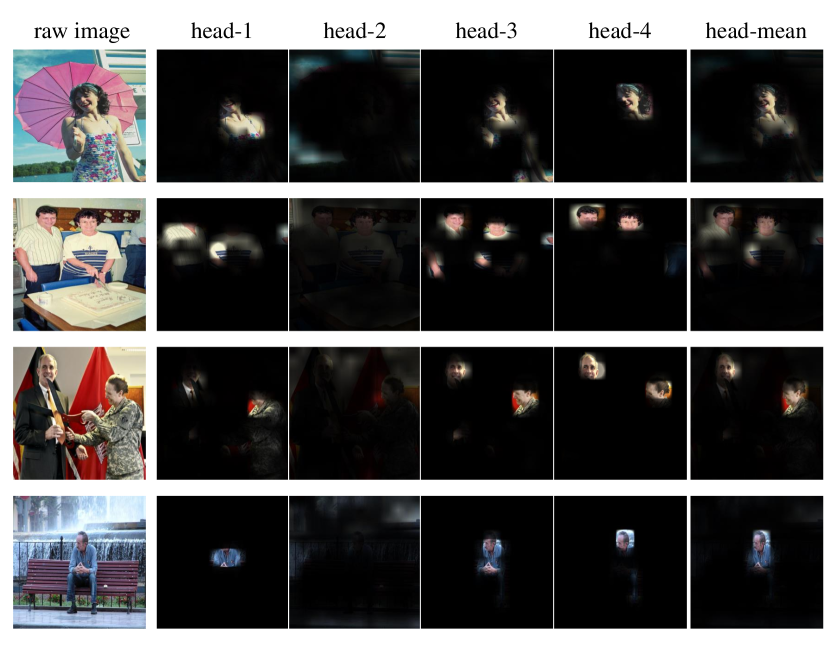
Figure 5: Visualization of multi-head attention maps for the target label person. Each column in the middle represents an attention map for one head and the rightmost column averages the maps of all heads. Best view in colors.

5 Conclusion

In this paper, we have presented a simple yet effective framework Query2Label (Q2L) for multi-label classification, which is developed based on Transformer decoders attached to an image classification backbone. The built-in cross-attention module in the Transformer decoder architecture offers an effective way to used label embeddings to query the existence of a class label and pool class-related features. The proposed framework consistently outperforms all prior works on several widely used data sets including MS-COCO, PASCAL VOC, NUSWIDE, and Visual Genome. We hope its simple model architecture and outstanding performance will serve as a strong baseline for future research on multi-label image classification.

Appendix A More Implementation Details

We adopt the official PyTorch implementation for both the backbone and Transformer modules [45]. Following DETR [3], we use 2D sine and cosine encodings to represent spatial positions. Each model was trained for $80$ epochs using Adam [29] and 1-cycle policy [43], with a maximal learning rate of $1e-4$. For regularization, we use Cutout [16] with a factor of 0.5 and True-wight-decay [38] of $1e-2$. Moreover, we normalize input images with mean $[0,0,0]$ and std $[1,1,1]$, and use RandAugment [12] for augmentation. Following common practices, we apply exponential moving average (EMA) to model parameters with a decay of $0.9997$. To speed up, we use mixed precision during model training. The entire code to reproduce the experiments will be made available.

Appendix B Metrics

Beyond the average precision (AP) and mean average precision (mAP), we report more metrics in the experiments, including the overall precision (OP), recall (OR), F1-measure (OF1) and per-category precision (CP), recall (CR), F1-measure (CF1). These metrics are computed as follows:

$$\mathrm{OP}=\frac{\sum_{i}M_{c}^{i}}{\sum_{i}M_{p}^{i}}, \mathrm{OR}=\frac{\sum_{i}M_{c}^{i}}{\sum_{i}M_{g}^{i}},$$ (6)

$$\mathrm{CP}=\frac{1}{C}\sum_{i}\frac{M_{c}^{i}}{M_{p}^{i}}, \mathrm{CR}=\frac{1}{C}\sum_{i}\frac{M_{c}^{i}}{M_{g}^{i}},$$

$$\mathrm{OF1}=\frac{2\times\mathrm{OP}\times\mathrm{OR}}{\mathrm{OP}+\mathrm{OR}}, \mathrm{CF1}=\frac{2\times\mathrm{CP}\times\mathrm{CR}}{\mathrm{CP}+\mathrm{CR}},$$

where $M_{c}^{i}$ is the number of images predicted correctly for the $i$-th category, $M_{p}^{i}$ is the number of images predicted for the $i$-th category, and $M_{g}^{i}$ is the number of ground truth images for the $i$-th category. For each image, we assign it a positive label if its prediction probability is greater than a threshold or negative otherwise. Note that these results may be affected by the chosen threshold. The $\mathrm{OF1}$ and $\mathrm{CF1}$ are the primary metrics among them, as they consider both recall and precision and are more comprehensive.

Appendix C Additional results on VOC07

We show the results with ImageNet-1k pretrained backbones only in the maintext for a fair comparison on VOC 07. Additional results are listed in Table 8.

Method	Resolution	mAP
TResNetL	448$\times$448	96.7
Q2L-TResL(Ours)	448$\times$448	96.9
Q2L-CvT(Ours)	384$\times$384	97.3

Table 8: Comparison of our method with prior state-of-the-art methods on VOC07. Backbones in all models are pretrained on ImageNet-22k dataset. All metrics are in %.

Appendix D More Visualization Results

We provide more visualization results of cross-attention maps on MS-COCO [35]. To visualize the cross-attention maps, we compute the attention values between labels and pixels. Since each matrix adds up to $1$ and each value in the matrix is small, we divide the entire matrix by $0.06$ and clip it between $0$ and $1$ to get a better visualization result. Then for a target label, we resize its corresponding attention value matrices (for multiple attention heads) to the same size as raw images and use the resized matrices as the opacity of each pixel in images. We plot the mean-head maps for more images in Fig. 6 and Fig. 7. These figures provide an intuitive explanation for the effectiveness of our spatial adaptive pooling and the superiority of our method. In addition, we show more multi-head attention maps of the target person in Fig. 8. We find that different heads are capable of focusing on different parts of targets.

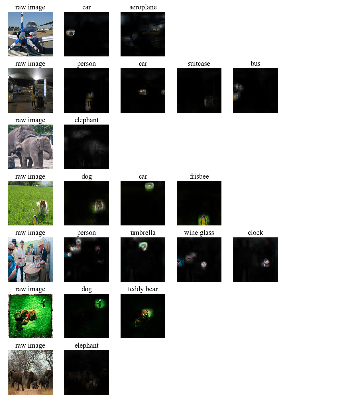
Figure 6: More visualizations of cross-attention maps. We plot the mean of each head’s cross-attention maps, which represent similarities of a given query and the extracted spatial features. Texts above images represent the ground truth labels (query) for the raw images. Best view in colors.

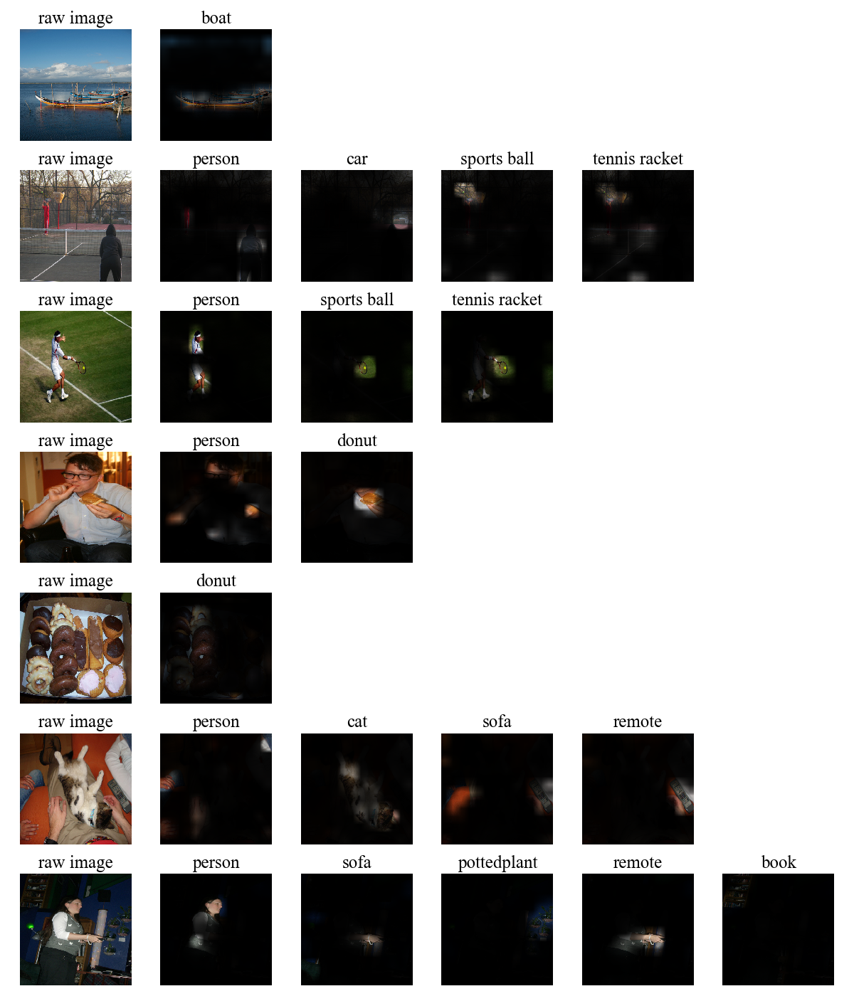
Figure 7: More visualizations of cross-attention maps (continued). Best view in colors.

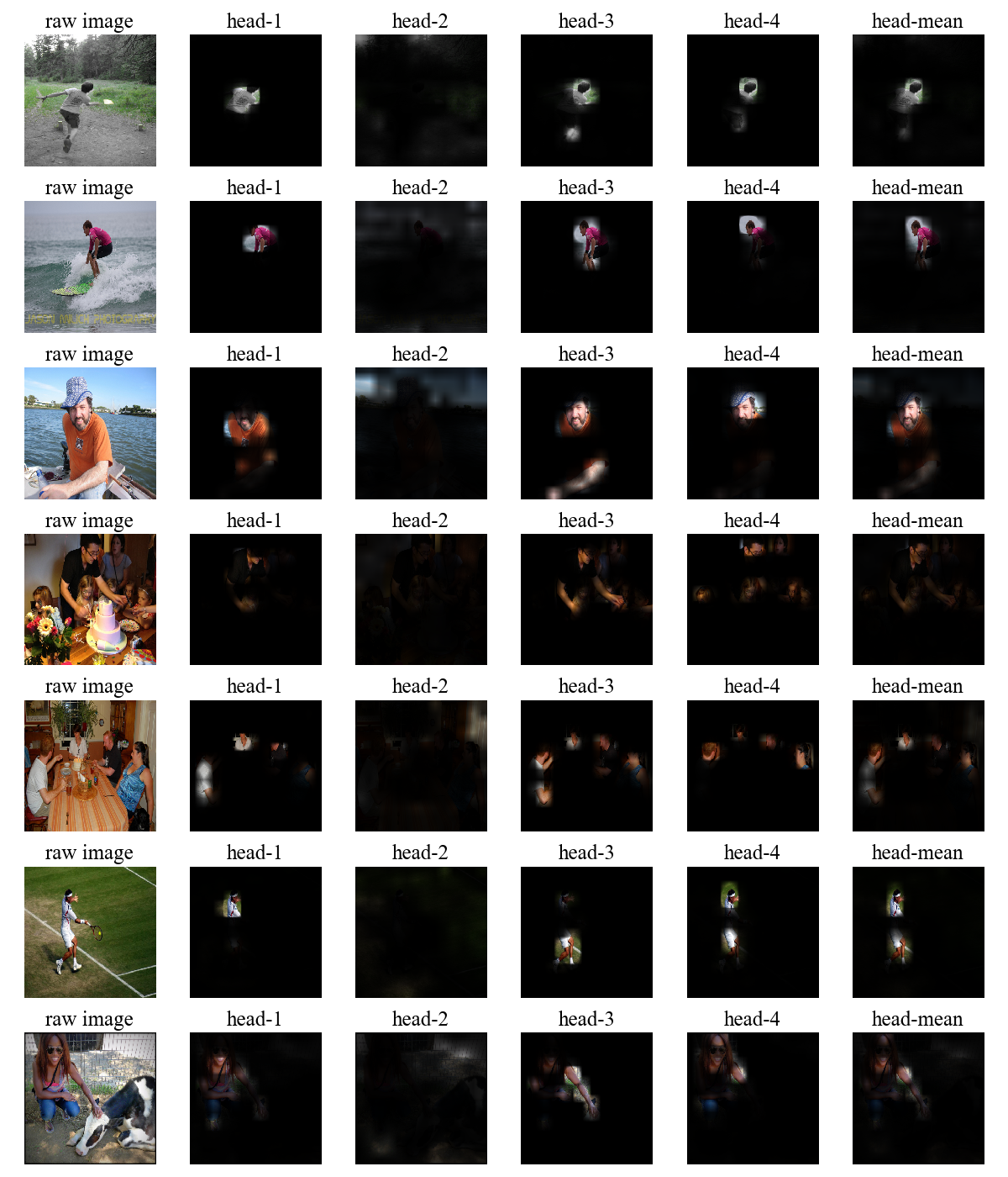
Figure 8: More visualizations of multi-head attention maps for the target label person. Each column in the middle represents an attention map for one head and the rightmost column averages the maps of all heads. Best view in colors.

References

- [1] Emanuel Ben-Baruch, Tal Ridnik, Nadav Zamir, Asaf Noy, Itamar Friedman, Matan Protter, and Lihi Zelnik-Manor. Asymmetric loss for multi-label classification, 2020.
- [2] Tom B. Brown, Benjamin Mann, Nick Ryder, Melanie Subbiah, Jared Kaplan, Prafulla Dhariwal, Arvind Neelakantan, Pranav Shyam, Girish Sastry, Amanda Askell, Sandhini Agarwal, Ariel Herbert-Voss, Gretchen Krueger, Tom Henighan, Rewon Child, Aditya Ramesh, Daniel M. Ziegler, Jeffrey Wu, Clemens Winter, Christopher Hesse, Mark Chen, Eric Sigler, Mateusz Litwin, Scott Gray, Benjamin Chess, Jack Clark, Christopher Berner, Sam McCandlish, Alec Radford, Ilya Sutskever, and Dario Amodei. Language models are few-shot learners. In Advances in Neural Information Processing Systems, volume 33, 2020.
- [3] Nicolas Carion, Francisco Massa, Gabriel Synnaeve, Nicolas Usunier, Alexander Kirillov, and Sergey Zagoruyko. End-to-end object detection with transformers. In European Conference on Computer Vision, pages 213–229. Springer, 2020.
- [4] Hanting Chen, Yunhe Wang, Tianyu Guo, Chang Xu, Yiping Deng, Zhenhua Liu, Siwei Ma, Chunjing Xu, Chao Xu, and Wen Gao. Pre-trained image processing transformer. arXiv preprint arXiv:2012.00364, 2020.
- [5] Mark Chen, Alec Radford, Rewon Child, Jeffrey Wu, Heewoo Jun, David Luan, and Ilya Sutskever. Generative pretraining from pixels. In International Conference on Machine Learning, pages 1691–1703. PMLR, 2020.
- [6] Tianshui Chen, Zhouxia Wang, Guanbin Li, and Liang Lin. Recurrent attentional reinforcement learning for multi-label image recognition. In Proceedings of the AAAI Conference on Artificial Intelligence, volume 32, 2018.
- [7] Tianshui Chen, Muxin Xu, Xiaolu Hui, Hefeng Wu, and Liang Lin. Learning semantic-specific graph representation for multi-label image recognition. In Proceedings of the IEEE/CVF International Conference on Computer Vision, pages 522–531, 2019.
- [8] Z. Chen, X. Wei, X. Jin, and Y. Guo. Multi-label image recognition with joint class-aware map disentangling and label correlation embedding. In 2019 IEEE International Conference on Multimedia and Expo (ICME), pages 622–627, 2019.
- [9] Zhao-Min Chen, Xiu-Shen Wei, Peng Wang, and Yanwen Guo. Multi-Label Image Recognition with Graph Convolutional Networks. In The IEEE Conference on Computer Vision and Pattern Recognition (CVPR), 2019.
- [10] Xing Cheng, Hezheng Lin, Xiangyu Wu, Fan Yang, Dong Shen, Zhongyuan Wang, Nian Shi, and Honglin Liu. Mltr: Multi-label classification with transformer, 2021.
- [11] Tat-Seng Chua, Jinhui Tang, Richang Hong, Haojie Li, Zhiping Luo, and Yantao Zheng. Nus-wide: a real-world web image database from national university of singapore. In Proceedings of the ACM International Conference on Image and Video Retrieval, page 48, 2009.
- [12] Ekin D Cubuk, Barret Zoph, Jonathon Shlens, and Quoc V Le. Randaugment: Practical automated data augmentation with a reduced search space. In Proceedings of the IEEE/CVF Conference on Computer Vision and Pattern Recognition Workshops, pages 702–703, 2020.
- [13] Zihang Dai, Zhilin Yang, Yiming Yang, Jaime G. Carbonell, Quoc Viet Le, and Ruslan Salakhutdinov. Transformer-xl: Attentive language models beyond a fixed-length context. In Proceedings of the 57th Annual Meeting of the Association for Computational Linguistics, pages 2978–2988, 2019.
- [14] Jia Deng, Wei Dong, Richard Socher, Li-Jia Li, Kai Li, and Li Fei-Fei. Imagenet: A large-scale hierarchical image database. In 2009 IEEE conference on computer vision and pattern recognition, pages 248–255. Ieee, 2009.
- [15] Jacob Devlin, Ming-Wei Chang, Kenton Lee, and Kristina N. Toutanova. Bert: Pre-training of deep bidirectional transformers for language understanding. In Proceedings of the 2019 Conference of the North American Chapter of the Association for Computational Linguistics: Human Language Technologies, Volume 1 (Long and Short Papers), pages 4171–4186, 2018.
- [16] Terrance DeVries and Graham W Taylor. Improved regularization of convolutional neural networks with cutout. arXiv preprint arXiv:1708.04552, 2017.
- [17] Alexey Dosovitskiy, Lucas Beyer, Alexander Kolesnikov, Dirk Weissenborn, Xiaohua Zhai, Thomas Unterthiner, Mostafa Dehghani, Matthias Minderer, Georg Heigold, Sylvain Gelly, et al. An image is worth 16x16 words: Transformers for image recognition at scale. arXiv preprint arXiv:2010.11929, 2020.
- [18] Mark Everingham, S. M. Eslami, Luc Gool, Christopher K. Williams, John Winn, and Andrew Zisserman. The pascal visual object classes challenge: A retrospective. International Journal of Computer Vision, 111(1):98–136, 2015.
- [19] Bin-Bin Gao and Hong-Yu Zhou. Learning to discover multi-class attentional regions for multi-label image recognition, 2020.
- [20] Bin-Bin Gao and Hong-Yu Zhou. Multi-label image recognition with multi-class attentional regions. arXiv preprint arXiv:2007.01755, 2020.
- [21] Zongyuan Ge, Dwarikanath Mahapatra, Suman Sedai, Rahil Garnavi, and Rajib Chakravorty. Chest x-rays classification: A multi-label and fine-grained problem. arXiv preprint arXiv:1807.07247, 2018.
- [22] Meng-Hao Guo, Jun-Xiong Cai, Zheng-Ning Liu, Tai-Jiang Mu, Ralph R Martin, and Shi-Min Hu. Pct: Point cloud transformer. arXiv preprint arXiv:2012.09688, 2020.
- [23] Meng-Hao Guo, Zheng-Ning Liu, Tai-Jiang Mu, and Shi-Min Hu. Beyond self-attention: External attention using two linear layers for visual tasks, 2021.
- [24] Kai Han, Yunhe Wang, Hanting Chen, Xinghao Chen, Jianyuan Guo, Zhenhua Liu, Yehui Tang, An Xiao, Chunjing Xu, Yixing Xu, et al. A survey on visual transformer. arXiv preprint arXiv:2012.12556, 2020.
- [25] Kaiming He, Xiangyu Zhang, Shaoqing Ren, and Jian Sun. Deep residual learning for image recognition. In Proceedings of the IEEE conference on computer vision and pattern recognition, pages 770–778, 2016.
- [26] Sepp Hochreiter and Jürgen Schmidhuber. Long short-term memory. Neural computation, 9(8):1735–1780, 1997.
- [27] Max Jaderberg, Karen Simonyan, Andrew Zisserman, and Koray Kavukcuoglu. Spatial transformer networks. arXiv preprint arXiv:1506.02025, 2015.
- [28] Salman Khan, Muzammal Naseer, Munawar Hayat, Syed Waqas Zamir, Fahad Shahbaz Khan, and Mubarak Shah. Transformers in vision: A survey. arXiv preprint arXiv:2101.01169, 2021.
- [29] Diederik P Kingma and Jimmy Ba. Adam: A method for stochastic optimization. arXiv preprint arXiv:1412.6980, 2014.
- [30] Ranjay Krishna, Yuke Zhu, Oliver Groth, Justin Johnson, Kenji Hata, Joshua Kravitz, Stephanie Chen, Yannis Kalantidis, Li-Jia Li, David A. Shamma, Michael S. Bernstein, and Li Fei-Fei. Visual genome: Connecting language and vision using crowdsourced dense image annotations. International Journal of Computer Vision, 123(1):32–73, 2017.
- [31] K. Lagler, M. Schindelegger, J. Böhm, H. Krásná, and T. Nilsson. Gpt2: Empirical slant delay model for radio space geodetic techniques. Geophysical Research Letters, 40(6):1069–1073, 2013.
- [32] Zhenzhong Lan, Mingda Chen, Sebastian Goodman, Kevin Gimpel, Piyush Sharma, and Radu Soricut. Albert: A lite bert for self-supervised learning of language representations. In ICLR 2020 : Eighth International Conference on Learning Representations, 2020.
- [33] Jack Lanchantin, Tianlu Wang, Vicente Ordonez, and Yanjun Qi. General multi-label image classification with transformers. arXiv preprint arXiv:2011.14027, 2020.
- [34] Tsung-Yi Lin, Priya Goyal, Ross Girshick, Kaiming He, and Piotr Dollár. Focal loss for dense object detection. In Proceedings of the IEEE international conference on computer vision, pages 2980–2988, 2017.
- [35] Tsung-Yi Lin, Michael Maire, Serge J. Belongie, James Hays, Pietro Perona, Deva Ramanan, Piotr Dollár, and C. Lawrence Zitnick. Microsoft coco: Common objects in context. In European Conference on Computer Vision, pages 740–755, 2014.
- [36] Yongcheng Liu, Lu Sheng, Jing Shao, Junjie Yan, Shiming Xiang, and Chunhong Pan. Multi-label image classification via knowledge distillation from weakly-supervised detection. In Proceedings of the 26th ACM international conference on Multimedia, pages 700–708, 2018.
- [37] Ze Liu, Yutong Lin, Yue Cao, Han Hu, Yixuan Wei, Zheng Zhang, Stephen Lin, and Baining Guo. Swin transformer: Hierarchical vision transformer using shifted windows, 2021.
- [38] Ilya Loshchilov and Frank Hutter. Decoupled weight decay regularization. arXiv preprint arXiv:1711.05101, 2017.
- [39] Tal Ridnik, Emanuel Ben-Baruch, Asaf Noy, and Lihi Zelnik-Manor. Imagenet-21k pretraining for the masses, 2021.
- [40] Tal Ridnik, Hussam Lawen, Asaf Noy, Emanuel Ben Baruch, Gilad Sharir, and Itamar Friedman. Tresnet: High performance gpu-dedicated architecture. Proceedings of the IEEE/CVF Winter Conference on Applications of Computer Vision, pages 1400–1409, 2020.
- [41] Jing Shao, Kai Kang, Chen Change Loy, and Xiaogang Wang. Deeply learned attributes for crowded scene understanding. In Proceedings of the IEEE conference on computer vision and pattern recognition, pages 4657–4666, 2015.
- [42] Karen Simonyan and Andrew Zisserman. Very deep convolutional networks for large-scale image recognition. In ICLR 2015 : International Conference on Learning Representations 2015, 2015.
- [43] Leslie N Smith. A disciplined approach to neural network hyper-parameters: Part 1–learning rate, batch size, momentum, and weight decay. arXiv preprint arXiv:1803.09820, 2018.
- [44] Aravind Srinivas, Tsung-Yi Lin, Niki Parmar, Jonathon Shlens, Pieter Abbeel, and Ashish Vaswani. Bottleneck transformers for visual recognition. arXiv preprint arXiv:2101.11605, 2021.
- [45] Ashish Vaswani, Noam Shazeer, Niki Parmar, Jakob Uszkoreit, Llion Jones, Aidan N Gomez, Lukasz Kaiser, and Illia Polosukhin. Attention is all you need. arXiv preprint arXiv:1706.03762, 2017.
- [46] Jiang Wang, Yi Yang, Junhua Mao, Zhiheng Huang, Chang Huang, and Wei Xu. Cnn-rnn: A unified framework for multi-label image classification. In 2016 IEEE Conference on Computer Vision and Pattern Recognition (CVPR), pages 2285–2294, 2016.
- [47] Zhouxia Wang, Tianshui Chen, Guanbin Li, Ruijia Xu, and Liang Lin. Multi-label image recognition by recurrently discovering attentional regions. In Proceedings of the IEEE international conference on computer vision, pages 464–472, 2017.
- [48] Yunchao Wei, Wei Xia, Min Lin, Junshi Huang, Bingbing Ni, Jian Dong, Yao Zhao, and Shuicheng Yan. Hcp: A flexible cnn framework for multi-label image classification. IEEE transactions on pattern analysis and machine intelligence, 38(9):1901–1907, 2015.
- [49] Haiping Wu, Bin Xiao, Noel Codella, Mengchen Liu, Xiyang Dai, Lu Yuan, and Lei Zhang. Cvt: Introducing convolutions to vision transformers, 2021.
- [50] Tong Wu, Qingqiu Huang, Ziwei Liu, Yu Wang, and Dahua Lin. Distribution-balanced loss for multi-label classification in long-tailed datasets. In European Conference on Computer Vision, pages 162–178. Springer, 2020.
- [51] Hao Yang, Joey Tianyi Zhou, Yu Zhang, Bin-Bin Gao, Jianxin Wu, and Jianfei Cai. Exploit bounding box annotations for multi-label object recognition. In Proceedings of the IEEE Conference on Computer Vision and Pattern Recognition, pages 280–288, 2016.
- [52] Jin Ye, Junjun He, Xiaojiang Peng, Wenhao Wu, and Yu Qiao. Attention-driven dynamic graph convolutional network for multi-label image recognition. In European Conference on Computer Vision, pages 649–665. Springer, 2020.
- [53] Renchun You, Zhiyao Guo, Lei Cui, Xiang Long, Yingze Bao, and Shilei Wen. Cross-modality attention with semantic graph embedding for multi-label classification. In Proceedings of the AAAI Conference on Artificial Intelligence, volume 34, pages 12709–12716, 2020.
- [54] Li Yuan, Yunpeng Chen, Tao Wang, Weihao Yu, Yujun Shi, Francis EH Tay, Jiashi Feng, and Shuicheng Yan. Tokens-to-token vit: Training vision transformers from scratch on imagenet. arXiv preprint arXiv:2101.11986, 2021.
- [55] Zhengyan Zhang, Xu Han, Zhiyuan Liu, Xin Jiang, Maosong Sun, and Qun Liu. Ernie: Enhanced language representation with informative entities. arXiv preprint arXiv:1905.07129, 2019.
- [56] Feng Zhu, Hongsheng Li, Wanli Ouyang, Nenghai Yu, and Xiaogang Wang. Learning spatial regularization with image-level supervisions for multi-label image classification. In Proceedings of the IEEE Conference on Computer Vision and Pattern Recognition, pages 5513–5522, 2017.
- [57] Xizhou Zhu, Weijie Su, Lewei Lu, Bin Li, Xiaogang Wang, and Jifeng Dai. Deformable detr: Deformable transformers for end-to-end object detection. arXiv preprint arXiv:2010.04159, 2020.