High-energy $\pi\pi$ scattering without and with photon radiation

Abstract

We discuss the processes $\pi\pi\to\pi\pi$ and $\pi\pi\to\pi\pi\gamma$ from a general quantum field theory (QFT) point of view. In the soft-photon limit where the photon energy $\omega\to 0$ we study the theorem due to F.E. Low. We confirm his result for the $1/\omega$ term of the $\pi\pi\to\pi\pi\gamma$ amplitude but disagree for the $\omega^{0}$ term. We analyse the origin of this discrepancy. Then we calculate the amplitudes for the above reactions in the tensor-pomeron model. We identify places where “anomalous” soft photons could come from. Three soft-photon approximations (SPAs) are introduced. The corresponding SPA results are compared to those obtained from the full tensor-pomeron model for c.m. energies $\sqrt{s}=10$ GeV and 100 GeV. The kinematic regions where the SPAs are a good representation of the full amplitude are determined. Finally we make some remarks on the type of fundamental information one could obtain from high-energy exclusive hadronic reactions without and with soft photon radiation.

I Introduction

In this paper we shall be concerned with photon emission in some strong-interaction processes. In particular, we shall consider soft photon emission, that is, the emission of photons with energy $\omega$ approaching zero. For this kinematic region there exists Low’s theorem Low:1958sn which is based strictly on Quantum Field Theory (QFT). The theorem states that for $\omega\to 0$ the photons come exclusively from the external hadrons in the process considered. But this poses immediately the question: how close do we have to come to $\omega=0$ in order to see the behaviour of the photon-emission amplitude predicted by Low?

There have been a number of experimental studies trying to verify Low’s theorem Goshaw:1979kq ; Chliapnikov:1984ed ; Botterweck:1991wf ; Banerjee:1992ut ; Antos:1993wv ; Tincknell:1996ks ; Belogianni:1997rh ; Belogianni:2002ib ; Belogianni:2002ic ; Abdallah:2005wn ; Abdallah:2007aa . For a review of the experimental situation see Wong:2014pY . The result is, that many experiments see rather large deviations from theoretical calculations in the soft-photon approximation (SPA) based on Low’s theorem. Clearly, this situation is unsatisfactory. This has motivated the feasibility study of measuring soft-photon phenomena in a next-generation experiment in the framework of the heavy-ion physics programme at the LHC for the 2030’s Adamova:2019vkf . Clearly, for preparing such soft-photon experiments accompanying theoretical studies are needed.

One class of hadronic reactions one can study at the LHC are exclusive diffractive proton-proton collisions. Examples are $pp$ elastic scattering and central exclusive production (CEP) reactions, for instance $pp\to p\pi^{+}\pi^{-}p$. In these reactions we can, of course, also have photon emission:

$$p+p\to p+p+\gamma\,,$$

$$p+p\to p+\pi^{+}+\pi^{-}+p+\gamma\,,$$ (1)

and we can study the soft-photon limit. The advantage of these exclusive diffractive reactions is that they are “clean” from the experimental side and that we have reasonable theoretical models for them. We shall work within the tensor-pomeron model as proposed in Ewerz:2013kda . There, the soft pomeron and the charge conjugation $C=+1$ reggeons are described as effective rank-2 symmetric tensor exchanges, the odderon and the $C=-1$ reggeons as effective vector exchanges. The tensor-pomeron model has been applied to quite a number of CEP reactions Lebiedowicz:2013ika ; Lebiedowicz:2014bea ; Lebiedowicz:2016ioh ; Lebiedowicz:2016zka ; Lebiedowicz:2018eui ; Lebiedowicz:2018sdt ; Lebiedowicz:2019jru ; Lebiedowicz:2019boz ; Lebiedowicz:2020yre ; Lebiedowicz:2021pzd which can and should all be studied by the present RHIC and LHC experiments Adam:2020sap ; McNulty:2017ejl ; Schicker:2019qcn ; Sirunyan:2019nog ; Sirunyan:2020cmr ; Sikora:2020mae . The next generation LHC experiment Adamova:2019vkf should be able to study these reactions in even greater detail, in particular, in the region of low transverse momenta. Applications of the model of Ewerz:2013kda have furthermore been made to photoproduction of $\pi^{+}\pi^{-}$ pairs Bolz:2014mya , a reaction which is also of interest for the LHC, and to deep-inelastic lepton-nucleon scattering at low $x$ Britzger:2019lvc . In Ewerz:2016onn it was shown that the experimental results Adamczyk:2012kn on the spin dependence of high-energy proton-proton elastic scattering exclude a scalar character of the pomeron couplings but are perfectly compatible with the tensor-pomeron model. A vector coupling for the pomeron could definitely be ruled out in Britzger:2019lvc .

With the present paper we want to start the theoretical study of soft photon emission in exclusive diffractive high-energy reactions in the TeV energy region in the framework of the tensor-pomeron model. Our first example will be, for simplicity, pion-pion elastic scattering. This is, of course, not easy to study for experiments. But, as we shall see, we can in this example compare our “exact” model results for photon emission to approximations based on Low’s theorem which gives the photon-emission amplitude to order $\omega^{-1}$ and $\omega^{0}$ in the photon energy $\omega$ for $\omega\to 0$. We shall show, as an important result, that the term of order $\omega^{0}$, presented in Low:1958sn , needs modifications.

Before coming to our present investigations we make remarks on some hadronic processes where photon emission has been studied, frequently using the soft-photon approximation.

Direct photons (i.e. photons which originate not from hadronic decays, but from inelastic scattering processes between partons) are an important electromagnetic probe of the quark-gluon plasma as created in heavy-ion collisions. Since pions are the dominant meson species produced in the heavy-ion collisions, the photon production via bremsstrahlung in pion-pion elastic collisions was found to be a very important source to interpret the data on the direct photon spectra and elliptic flow simultaneously Linnyk:2013hta ; Linnyk:2013wma . In Linnyk:2013hta ; Linnyk:2013wma the SPA was used and, therefore, the resulting yield of the bremsstrahlung photons depends on some model assumptions.

The description of the photon bremsstrahlung in meson-meson scattering beyond the SPA, within the one-boson exchange (OBE) model, was discussed for the first time in Eggers:1995jq and applied to the dilepton bremsstrahlung in pion-pion collisions. Later on, in Liu:2007zzw , it was applied to the low-energy photon bremsstrahlung in pion-pion and kaon-kaon collisions. Within the OBE model the interaction of pions is described by three resonance exchanges $\sigma$, $\rho$ and $f_{2}(1270)$ in the $t$, $u$ and $s$ channels (the $u$ channel diagrams are needed only in the case of identical pions).

In Linnyk:2015tha ; Linnyk:2015rco the authors applied the covariant OBE effective (chiral) model for the pion-pion scattering. The “exact” OBE model result of the invariant rate of photon bremsstrahlung was compared with that of the SPA. It was noted there that the accuracy of the SPA approximation can be significantly improved and the region of its applicability can be extended by evaluating the on-shell elastic cross section not at the c.m. energy $\sqrt{s}$ of the $\pi\pi\to\pi\pi\gamma$ process but at a certain smaller energy. One can see in Fig. 6 of Linnyk:2015tha (or Fig. 21 of Linnyk:2015rco ) that the “improved SPA model” gives a good approximation to the “exact” OBE result up to photon energies $\approx 2$ GeV. There the dominant contribution to the rates comes from low collision energies $\sqrt{s}$. The deviation between the OBE result and that calculated within the improved SPA is most pronounced at high $\sqrt{s}$ and high photon energies.

Whereas the examples of photon radiation discussed above concerned low energy reactions, there have, of course, also been studies of photon radiation for exclusive reactions at the LHC. Exclusive diffractive photon bremsstrahlung in proton-proton collisions was discussed in Khoze:2010jv ; Lebiedowicz:2013xlb . Feasibility studies of the measurement of the exclusive diffractive bremsstrahlung cross section in proton-proton collisions at the center-of-mass energy $\sqrt{s}=13$ TeV at the LHC were performed in Chwastowski:2016jkl ; Chwastowski:2016zzl .

Very interesting general investigations of photon emission in hadronic reactions have been presented, for instance, in Gribov:1966hs ; Lipatov:1988ii ; DelDuca:1990gz ; Gervais:2017yxv ; Bern:2014vva ; Lysov:2014csa . We shall comment on results given in these papers below, as far as they have a bearing on our own investigations.

Now we list the high-energy reactions which we want to study in our present paper. In Sec. II we discuss the reactions $\pi^{-}\pi^{0}\to\pi^{-}\pi^{0}$ and $\pi^{-}\pi^{0}\to\pi^{-}\pi^{0}\gamma$ from a general QFT point of view. Section III deals with the limit of photon-energy $\omega\to 0$ and we discuss the terms in the amplitude of orders $\omega^{-1}$ and $\omega^{0}$. In Sec. IV we introduce our model for $\pi^{\mp}\pi^{0}$ and charged-pion scattering and for the corresponding reactions with photon emission. Section V is devoted to a comparison of our “exact” model results to various approximations based Low’s theorem. In Sec. VI we give our conclusions and an outlook on further work. In Appendix A we compare in detail our results for the terms of order $\omega^{-1}$ and $\omega^{0}$ in the photon emission amplitude to results presented in the literature. In Appendix B we discuss the cross section $d\sigma/d\omega$ for $\omega\to 0$.

II General properties of the reactions $\pi\pi\to\pi\pi$ and $\pi\pi\to\pi\pi\gamma$

Here we study general QFT relations for pion-pion elastic scattering without and with photon radiation. We shall work to leading order in the electromagnetic coupling. For simplicity we shall consider $\pi^{-}\pi^{0}$ scattering, that is, the reactions

$$\pi^{-}(p_{a})+\pi^{0}(p_{b})\to\pi^{-}(p_{1})+\pi^{0}(p_{2})\,,$$ (2)

$$\pi^{-}(p_{a})+\pi^{0}(p_{b})\to\pi^{-}(p_{1}^{\prime})+\pi^{0}(p_{2}^{\prime})+\gamma(k,\epsilon)\,.$$ (3)

Here $p_{a}$, $p_{b}$, $p_{1}$, $p_{2}$, $p_{1}^{\prime}$, $p_{2}^{\prime}$ and $k$ are the momenta of the particles and $\epsilon$ is the polarisation vector of the photon, respectively. The energy-momentum conservation in (2) and (3) requires

$$p_{a}+p_{b}=p_{1}+p_{2}\,,$$ (4)

$$p_{a}+p_{b}=p_{1}^{\prime}+p_{2}^{\prime}+k\,.$$ (5)

We denote the amplitude for the reaction (2) by

$${\cal T}(p_{a},p_{b},p_{1},p_{2})=\braket{\pi^{-}(p_{1}),\pi^{0}(p_{2})}{{\cal T}}{\pi^{-}(p_{a}),\pi^{0}(p_{b})}\,.$$ (6)

Since pions have $G$ parity $-1$ all diagrams for (6) are one-particle irreducible. In QFT we can extend the amplitude (6) for off shell pions (Fig. 1).

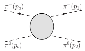
Figure 1: Diagram for the off shell $\pi^{-}\pi^{0}$ scattering amplitude.

This off shell scattering amplitude will still satisfy the energy-momentum conservation (4) and can only depend on the following 6 variables

$$s_{L}=p_{a}\cdot p_{b}+p_{1}\cdot p_{2}\,,$$

$$t=(p_{a}-p_{1})^{2}=(p_{b}-p_{2})^{2}\,,$$

$$m_{a}^{2}=p_{a}^{2}\,,\;\,m_{b}^{2}=p_{b}^{2}\,,\;\,m_{1}^{2}=p_{1}^{2}\,,\;\,m_{2}^{2}=p_{2}^{2}\,.$$ (7)

Here we use as squared energy variable $s_{L}$, following Low:1958sn , instead of the more usual Mandelstam variable $s$. We have

$$s=s_{L}+\frac{1}{2}\left(m_{a}^{2}+m_{b}^{2}+m_{1}^{2}+m_{2}^{2}\right)\,.$$ (8)

The on- or off-shell amplitude corresponding to (6) as a function of the variables (7) will be denoted by

$${\cal M}^{(0)}(s_{L},t,m_{a}^{2},m_{b}^{2},m_{1}^{2},m_{2}^{2})=\left.{\cal T}(p_{a},p_{b},p_{1},p_{2})\right|_{\rm on\;shell\;or\;off\;shell}.$$ (9)

The on-shell amplitude (6) is then ${\cal M}^{(0)}(s_{L},t,m_{\pi}^{2},m_{\pi}^{2},m_{\pi}^{2},m_{\pi}^{2})$.

Next we study the reaction (3) where we have two one-particle reducible diagrams (Figs. 2 (a), (b)) and one irreducible diagram (Fig. 2 (c)).

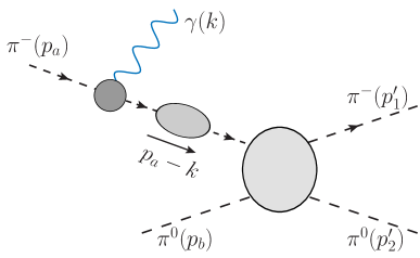
(a)      (b)
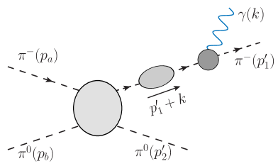
(c)

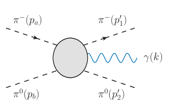
Figure 2: One-particle reducible (a, b) and irreducible (c) diagrams for $\pi^{-}\pi^{0}\to\pi^{-}\pi^{0}\gamma$.

For the diagrams (a) and (b) we need the off-shell $\pi\pi$ amplitude (9), the pion propagator $\Delta(p^{2})$ and the pion-photon vertex function $\Gamma_{\lambda}(p^{\prime},p)$:

$$i\Delta(p^{2})\,,$$ (10)

$$ie\Gamma_{\lambda}(p^{\prime},p)\,.$$ (11)

We denote by $e=\sqrt{4\pi\alpha}>0$ the $\pi^{+}$ charge.

The expressions for the amplitudes of Figs. 2 (a, b) can be written as follows:

$${\cal M}_{\lambda}^{(a)}=-e\,{\cal M}^{(0,\,a)}\,\Delta[(p_{a}-k)^{2}]\,\Gamma_{\lambda}(p_{a}-k,p_{a})\,,$$

$${\cal M}^{(0,\,a)}={\cal M}^{(0)}[(p_{a}-k,p_{b})+p_{1}^{\prime}\cdot p_{2}^{\prime},(p_{b}-p_{2}^{\prime})^{2},(p_{a}-k)^{2},m_{\pi}^{2},m_{\pi}^{2},m_{\pi}^{2}],$$ (12)

$${\cal M}_{\lambda}^{(b)}=-e\,\Gamma_{\lambda}(p_{1}^{\prime},p_{1}^{\prime}+k)\,\Delta[(p_{1}^{\prime}+k)^{2}]\,{\cal M}^{(0,\,b)}\,,$$

$${\cal M}^{(0,\,b)}={\cal M}^{(0)}[p_{a}\cdot p_{b}+(p_{1}^{\prime}+k,p_{2}^{\prime}),(p_{b}-p_{2}^{\prime})^{2},m_{\pi}^{2},m_{\pi}^{2},(p_{1}^{\prime}+k)^{2},m_{\pi}^{2}].$$ (13)

The photon-emission amplitude is

$$\braket{\gamma(k,\epsilon),\pi^{-}(p_{1}^{\prime}),\pi^{0}(p_{2}^{\prime})}{{\cal T}}{\pi^{-}(p_{a}),\pi^{0}(p_{b})}=(\epsilon^{\lambda})^{*}\,{\cal M}_{\lambda}$$ (14)

where

$${\cal M}_{\lambda}={\cal M}_{\lambda}^{(a)}+{\cal M}_{\lambda}^{(b)}+{\cal M}_{\lambda}^{(c)}\,.$$ (15)

${\cal M}_{\lambda}$ also determines the emission of virtual photons of mass $k^{2}>0$ which then decay to a lepton pair. For $k^{2}<0$ ${\cal M}_{\lambda}$ enters the amplitude for the 3-body reaction $e^{\pm}\pi^{-}\pi^{0}\to e^{\pm}\pi^{-}\pi^{0}$. The amplitude ${\cal M}_{\lambda}$ must satisfy the gauge-invariance relation, valid for all $k^{2}$,

$$k^{\lambda}{\cal M}_{\lambda}=k^{\lambda}\left({\cal M}_{\lambda}^{(a)}+{\cal M}_{\lambda}^{(b)}+{\cal M}_{\lambda}^{(c)}\right)=0\,,$$ (16)

that is, we have

$$k^{\lambda}{\cal M}_{\lambda}^{(c)}=-k^{\lambda}{\cal M}_{\lambda}^{(a)}-k^{\lambda}{\cal M}_{\lambda}^{(b)}\,.$$ (17)

We shall now use (12), (13), and (17), to get a simple relation between $k^{\lambda}{\cal M}_{\lambda}^{(c)}$ and ${\cal M}^{(0,\,a)}$, ${\cal M}^{(0,\,b)}$. For this we recall the normalisation conditions for the pion propagator and the vertex function. We have

$$\left.\Delta^{-1}(p^{2})\right|_{p^{2}=m_{\pi}^{2}}=0\,,\quad\frac{\partial}{\partial p^{2}}\left.\Delta^{-1}(p^{2})\right|_{p^{2}=m_{\pi}^{2}}=1\,,$$

$$\left.\Gamma_{\lambda}(p^{\prime},p)\right|_{p^{\prime}=p,p^{2}=m_{\pi}^{2}}=2p_{\lambda}\,.$$ (18)

Furthermore we have the Ward-Takahashi identity Ward:1950xp ; Takahashi:1957xn ,

$$(p^{\prime}-p)^{\lambda}\Gamma_{\lambda}(p^{\prime},p)=\Delta^{-1}(p^{\prime 2})-\Delta^{-1}(p^{2})\,.$$ (19)

From (18) and (19) we obtain for $p_{a}^{2}=m_{\pi}^{2}$

$$\Delta[(p_{a}-k)^{2}]\,\Gamma_{\lambda}(p_{a}-k,p_{a})\,k^{\lambda}$$

$$\qquad\qquad=-\Delta[(p_{a}-k)^{2}]\,\Gamma_{\lambda}(p_{a}-k,p_{a})\,(p_{a}-k-p_{a})^{\lambda}$$

$$\qquad\qquad=-\Delta[(p_{a}-k)^{2}]\,\{\Delta^{-1}[(p_{a}-k)^{2}]-\Delta^{-1}[p_{a}^{2}]\}$$

$$\qquad\qquad=-1\,.$$ (20)

Similarly we get for $p_{1}^{\prime 2}=m_{\pi}^{2}$

$$k^{\lambda}\,\Gamma_{\lambda}(p_{1}^{\prime},p_{1}^{\prime}+k)\,\Delta[(p_{1}^{\prime}+k)^{2}]$$

$$\qquad\qquad=-[p_{1}^{\prime}-(p_{1}^{\prime}+k)]^{\lambda}\,\Gamma_{\lambda}(p_{1}^{\prime},p_{1}^{\prime}+k)\,\Delta[(p_{1}^{\prime}+k)^{2}]$$

$$\qquad\qquad=-\{\Delta^{-1}[p_{1}^{\prime 2}]-\Delta^{-1}[(p_{1}^{\prime}+k)^{2}]\}\,\Delta[(p_{1}^{\prime}+k)^{2}]$$

$$\qquad\qquad=1\,.$$ (21)

From (12), (13), (17), (20), and (21), we obtain

$$k^{\lambda}{\cal M}_{\lambda}^{(a)}=e\,{\cal M}^{(0,\,a)}\,,$$

$$k^{\lambda}{\cal M}_{\lambda}^{(b)}=-e\,{\cal M}^{(0,\,b)}\,,$$ (22)

$$k^{\lambda}{\cal M}_{\lambda}^{(c)}=-e\,{\cal M}^{(0,\,a)}+e\,{\cal M}^{(0,\,b)}\,,$$ (23)

where ${\cal M}^{(0,\,a)}$ and ${\cal M}^{(0,\,b)}$ are given explicitly in (12) and (13), respectively.

III The expansion of the photon-emission amplitude to the order $\omega^{-1}$ plus $\omega^{0}$

In this section we discuss the expansion of the amplitude ${\cal M}_{\lambda}$ (15) to the orders $\omega^{-1}$ and $\omega^{0}$. Here $\omega=k^{0}$ and, if not stated otherwise, we work in the overall c.m. system of the reaction (3). We shall in the following assume that all components of the photon momentum are proportional to $\omega$, $k^{\mu}\propto\omega$, with $\omega\to 0$. This is perfectly alright theoretically, but can this also be realised in nature? For real photon emission, $k^{2}=0$, this clearly can be realised. It is also possible for $k^{2}<0$ in the 3-body collision

$$e^{\pm}+\pi^{-}+\pi^{0}\to e^{\pm}+\pi^{-}+\pi^{0}\,.$$ (24)

For $k^{2}>0$ we can have $e^{+}e^{-}$ production

$$\pi^{-}+\pi^{0}\to e^{+}+e^{-}+\pi^{-}+\pi^{0}\,.$$ (25)

But here $\omega\geqslant 2m_{e}$ and $k^{2}\geqslant 4m_{e}^{2}$, with $m_{e}$ the electron mass. Thus, in (25) we cannot reach $\omega=0$. But the electron mass is very small on a hadronic scale, $m_{e}\simeq 0.5$ MeV, and, therefore, the limit $\omega\to 0$ should also be of relevance for the reaction (25).

We start our investigation of the small $\omega$ limit with the pion propagator (10). We are working to lowest order in the electromagnetic coupling. Thus, $\Delta^{-1}(p^{2})$ is for us a purely hadronic object. Its nearest singularity to $p^{2}=0$ is at $p^{2}=(3m_{\pi})^{2}$ as we see from the Landau conditions (cf. for instance Bjorken:1965 ). Therefore, we can expand $\Delta^{-1}(p^{2})$ around $p^{2}=m_{\pi}^{2}$ as follows with $c$ a constant:

$$\Delta^{-1}(p^{2})=p^{2}-m_{\pi}^{2}+c(p^{2}-m_{\pi}^{2})^{2}+\ldots\,.$$ (26)

This gives for $p_{a}^{2}=m_{\pi}^{2}$ and $p_{1}^{\prime 2}=m_{\pi}^{2}$ the following

$$\Delta^{-1}[(p_{a}-k)^{2}]=(-2p_{a}\cdot k+k^{2})[1+c(-2p_{a}\cdot k+k^{2})+{\cal O}(\omega^{2})]\,,$$

$$\Delta[(p_{a}-k)^{2}]=\frac{1}{-2p_{a}\cdot k+k^{2}}[1-c(-2p_{a}\cdot k+k^{2})+{\cal O}(\omega^{2})]\,,$$ (27)

$$\Delta^{-1}[(p_{1}^{\prime}+k)^{2}]=(2p_{1}^{\prime}\cdot k+k^{2})[1+c(2p_{1}^{\prime}\cdot k+k^{2})+{\cal O}(\omega^{2})]\,,$$

$$\Delta[(p_{1}^{\prime}+k)^{2}]=\frac{1}{2p_{1}^{\prime}\cdot k+k^{2}}[1-c(2p_{1}^{\prime}\cdot k+k^{2})+{\cal O}(\omega^{2})]\,.$$ (28)

From (12), (13) and (15) we see that we must now expand $\Gamma_{\lambda}$, ${\cal M}^{(0,\,a)}$ and ${\cal M}^{(0,\,b)}$ up to order $\omega$ and ${\cal M}_{\lambda}^{(c)}$ up to order $\omega^{0}$ for getting the total amplitude ${\cal M}_{\lambda}$ expanded up to order $\omega^{0}$.

We start with $\Gamma_{\lambda}(p^{\prime},p)$ which has the general expansion

$$\Gamma_{\lambda}(p^{\prime},p) = (p^{\prime}+p)_{\lambda}\,A[p^{\prime 2}-m_{\pi}^{2},p^{2}-m_{\pi}^{2},(p^{\prime}-p)^{2}]$$ (29)

$$+(p^{\prime}-p)_{\lambda}\,B[p^{\prime 2}-m_{\pi}^{2},p^{2}-m_{\pi}^{2},(p^{\prime}-p)^{2}]\,.$$

The functions $A$ and $B$ are analytic in their variables in the region of interest to us as we see again from the Landau conditions. The Ward-Takahashi identity gives

$$(p^{\prime}-p)^{\lambda}\,\Gamma_{\lambda}(p^{\prime},p) = (p^{\prime 2}-p^{2})\,A[p^{\prime 2}-m_{\pi}^{2},p^{2}-m_{\pi}^{2},(p^{\prime}-p)^{2}]$$ (30)

$$+(p^{\prime}-p)^{2}\,B[p^{\prime 2}-m_{\pi}^{2},p^{2}-m_{\pi}^{2},(p^{\prime}-p)^{2}]$$

$$= \Delta^{-1}(p^{\prime 2})-\Delta^{-1}(p^{2})\,.$$

Now we set in (30) $p=p_{a}$, $p^{\prime}=p_{a}-k$, $p_{a}^{2}=m_{\pi}^{2}$ and get

$$(p^{\prime 2}-m_{\pi}^{2})\,A(p^{\prime 2}-m_{\pi}^{2},0,k^{2})+k^{2}\,B(p^{\prime 2}-m_{\pi}^{2},0,k^{2})$$

$$\qquad=\Delta^{-1}(p^{\prime 2})=p^{\prime 2}-m_{\pi}^{2}+c(p^{\prime 2}-m_{\pi}^{2})^{2}+\ldots\,.$$ (31)

Therefore, we must have

$$B(p^{\prime 2}-m_{\pi}^{2},0,k^{2})=(p^{\prime 2}-m_{\pi}^{2})\,\tilde{B}(p^{\prime 2}-m_{\pi}^{2},k^{2})$$ (32)

and we get with $p^{\prime 2}-m_{\pi}^{2}=-2p_{a}\cdot k+k^{2}$

$$A(-2p_{a}\cdot k+k^{2},0,k^{2})=1+c(-2p_{a}\cdot k+k^{2})+{\cal O}(\omega^{2})\,,$$

$$B(-2p_{a}\cdot k+k^{2},0,k^{2})={\cal O}(\omega)\,.$$ (33)

Inserting (33) in (29) we find

$$\Gamma_{\lambda}(p_{a}-k,p_{a})=(2p_{a}-k)_{\lambda}[1+c(-2p_{a}\cdot k+k^{2})]+{\cal O}(\omega^{2})\,.$$ (34)

In a completely analogous way we get for $p_{1}^{\prime 2}=m_{\pi}^{2}$

$$\Gamma_{\lambda}(p_{1}^{\prime},p_{1}^{\prime}+k)=(2p_{1}^{\prime}+k)_{\lambda}[1+c(2p_{1}^{\prime}\cdot k+k^{2})]+{\cal O}(\omega^{2})\,.$$ (35)

From (27), (28), (34) and (35) we get

$$\Delta[(p_{a}-k)^{2}]\,\Gamma_{\lambda}(p_{a}-k,p_{a})=\frac{(2p_{a}-k)_{\lambda}}{-2p_{a}\cdot k+k^{2}}+{\cal O}(\omega)\,,$$ (36)

$$\Gamma_{\lambda}(p_{1}^{\prime},p_{1}^{\prime}+k)\,\Delta[(p_{1}^{\prime}+k)^{2}]=\frac{(2p_{1}^{\prime}+k)_{\lambda}}{2p_{1}^{\prime}\cdot k+k^{2}}+{\cal O}(\omega)\,.$$ (37)

Next we investigate the energy-momentum conservation conditions (4) and (5) for the reactions (2) and (3), respectively. It is clear that for $k\neq 0$ we cannot have $p_{1}=p_{1}^{\prime}$ and $p_{2}=p_{2}^{\prime}$ since

$$p_{a}+p_{b}\neq p_{1}+p_{2}+k\,.$$ (38)

This means that when going from (2) to (3) we must have a change of momenta $p_{1}\to p_{1}^{\prime}\neq p_{1}$ and $p_{2}\to p_{2}^{\prime}\neq p_{2}$. In fact, choosing for the reaction (3) some $k\neq 0$, even a small momentum $k$, this does not fix $p_{1}^{\prime}$ and $p_{2}^{\prime}$. This is best seen in the rest system of the four-vector $p_{a}+p_{b}-k$. There we have $\mbox{\boldmath$p_{1}^{\prime}$}+\mbox{\boldmath$p_{2}^{\prime}$}=0$, $|\mbox{\boldmath$p_{1}^{\prime}$}|$ is fixed and thus $p_{1}^{\prime}$ can still vary on a sphere of radius $|\mbox{\boldmath$p_{1}^{\prime}$}|$. For the following we work, however, in the overall c.m. system of reaction (3).

We write

$$p_{1}^{\prime}=p_{1}-l_{1}\,,\quad p_{2}^{\prime}=p_{2}-l_{2}\,,$$ (39)

and get from (4) and (5) the conditions

$$l_{1}+l_{2}=k\,,\quad(p_{1}-l_{1})^{2}=m_{\pi}^{2}\,,\quad(p_{2}-l_{2})^{2}=m_{\pi}^{2}\,.$$ (40)

For given $k$ these are 6 conditions for the 8 unknowns $l_{1}$, $l_{2}$ giving a 2-parameter solution as it should be. Working in the common c.m. system of the reactions (2) and (3) we set with $\mbox{\boldmath$\hat{p}_{1}$}=\mbox{\boldmath$p_{1}$}/|\mbox{\boldmath$p_{1}$}|$

$$(l_{1}^{\mu})=\left(\begin{array}[]{l}l_{1}^{0}\\ l_{1\parallel}\mbox{\boldmath$\hat{p}_{1}$}+\mbox{\boldmath$l_{1\perp}$}\\ \end{array}\right)\,,\quad\mbox{\boldmath$l_{1\perp}$}\cdot\mbox{\boldmath$\hat{p}_{1}$}=0\,,$$ (43)

$$(l_{2}^{\mu})=\left(\begin{array}[]{l}l_{2}^{0}\\ l_{2\parallel}\mbox{\boldmath$\hat{p}_{1}$}+\mbox{\boldmath$l_{2\perp}$}\\ \end{array}\right)\,,\quad\mbox{\boldmath$l_{2\perp}$}\cdot\mbox{\boldmath$\hat{p}_{1}$}=0\,,$$ (46)

$$(k^{\mu})=\left(\begin{array}[]{l}\omega\\ k_{\parallel}\mbox{\boldmath$\hat{p}_{1}$}+\mbox{\boldmath$k_{\perp}$}\\ \end{array}\right)\,,\quad\mbox{\boldmath$k_{\perp}$}\cdot\mbox{\boldmath$\hat{p}_{1}$}=0\,.$$ (49)

Inserting this in (40) we get the system of equations

$$l_{2}=k-l_{1}\,,$$

$$p_{1}^{0}l_{1}^{0}-|\mbox{\boldmath$p_{1}$}|l_{1\parallel}=\frac{1}{2}l_{1}^{2}\,,$$

$$p_{1}^{0}l_{1}^{0}+|\mbox{\boldmath$p_{1}$}|l_{1\parallel}=p_{1}^{0}k^{0}+|\mbox{\boldmath$p_{1}$}|k_{\parallel}-\frac{1}{2}(k-l_{1})^{2}\,.$$ (50)

Now we make an important choice for the following. We assume that together with the soft photon emitted with energy $\omega\to 0$ we consider only slight changes of the momenta $p_{1}\to p_{1}^{\prime}$ and $p_{2}\to p_{2}^{\prime}$. That is, we assume

$$l_{1}^{\mu}={\cal O}(\omega)\,,\quad l_{2}^{\mu}={\cal O}(\omega)\,.$$ (51)

With this we can neglect the quadratic terms in $l_{1}$, $l_{2}$, $k$ in (50). The solution of the resulting equations is

$$(l_{1}^{\mu})=\left(\begin{array}[]{l}\dfrac{1}{2p_{1}^{0}}(p_{2}\cdot k)\\ \dfrac{1}{2|\mbox{\boldmath$p_{1}$}|}\mbox{\boldmath$\hat{p}_{1}$}(p_{2}\cdot k)+\mbox{\boldmath$l_{1\perp}$}\\ \end{array}\right),$$ (54)

$$(l_{2}^{\mu})=\left(\begin{array}[]{l}\dfrac{1}{2p_{1}^{0}}(p_{1}\cdot k)\\ \mbox{\boldmath$k$}-\dfrac{1}{2|\mbox{\boldmath$p_{1}$}|}\mbox{\boldmath$\hat{p}_{1}$}(p_{2}\cdot k)-\mbox{\boldmath$l_{1\perp}$}\\ \end{array}\right).$$ (57)

Here $l_{1\perp}$ stays undetermined, corresponding to the 2-parameter freedom of the momenta $p_{1}^{\prime}$, $p_{2}^{\prime}$ for given $k$. This is illustrated in Fig. 3. In the order of $\omega$ considered we get

$$p_{1}\cdot l_{1}=0\,,\quad p_{2}\cdot l_{2}=0\,.$$ (58)

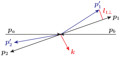
Figure 3: Illustration of the momentum configurations for $\pi^{-}\pi^{0}\to\pi^{-}\pi^{0}$ (2) and $\pi^{-}\pi^{0}\to\pi^{-}\pi^{0}\gamma$ (3) in the c.m. system.

Now we can expand ${\cal M}^{(0,\,a)}$ (12) and ${\cal M}^{(0,\,b)}$ (13) up to order $\omega$. We get with $s_{L}$ and $t$ from (7),

$${\cal M}^{(0,\,a)} = {\cal M}^{(0)}[(p_{a}-k,p_{b})+p_{1}^{\prime}\cdot p_{2}^{\prime},(p_{b}-p_{2}^{\prime})^{2},(p_{a}-k)^{2},m_{\pi}^{2},m_{\pi}^{2},m_{\pi}^{2}]$$ (59)

$$= {\cal M}^{(0)}[s_{L}-(p_{b}+p_{1},k)-(p_{2}\cdot l_{1}),t-2(p_{a}-p_{1},k-l_{1}),m_{\pi}^{2}-2(p_{a}\cdot k),m_{\pi}^{2},m_{\pi}^{2},m_{\pi}^{2}]$$

$$+{\cal O}(\omega^{2})$$

$$= \big{\{}1-\left[(p_{b}+p_{1},k)+(p_{2}\cdot l_{1})\right]\frac{\partial}{\partial s_{L}}-\left[2(p_{a}-p_{1},k)-2(p_{a}\cdot l_{1})\right]\frac{\partial}{\partial t}-2(p_{a}\cdot k)\frac{\partial}{\partial m_{a}^{2}}\big{\}}$$

$$\times\left.{\cal M}^{(0)}(s_{L},t,m_{a}^{2},m_{\pi}^{2},m_{\pi}^{2},m_{\pi}^{2})\right|_{m_{a}^{2}=m_{\pi}^{2}}+{\cal O}(\omega^{2})\,,$$

$${\cal M}^{(0,\,b)} = {\cal M}^{(0)}[p_{a}\cdot p_{b}+(p_{1}^{\prime}+k,p_{2}^{\prime}),(p_{b}-p_{2}^{\prime})^{2},m_{\pi}^{2},m_{\pi}^{2},(p_{1}^{\prime}+k)^{2},m_{\pi}^{2}]$$ (60)

$$= {\cal M}^{(0)}[s_{L}-(p_{1}\cdot k),t-2(p_{a}-p_{1},k)+2(p_{a}\cdot l_{1}),m_{\pi}^{2},m_{\pi}^{2},m_{\pi}^{2}+2(p_{1}\cdot k),m_{\pi}^{2}]$$

$$+{\cal O}(\omega^{2})$$

$$= \big{\{}1-(p_{1}\cdot k)\frac{\partial}{\partial s_{L}}-\left[2(p_{a}-p_{1},k)-2(p_{a}\cdot l_{1})\right]\frac{\partial}{\partial t}+2(p_{1}\cdot k)\frac{\partial}{\partial m_{1}^{2}}\big{\}}$$

$$\times\left.{\cal M}^{(0)}(s_{L},t,m_{\pi}^{2},m_{\pi}^{2},m_{1}^{2},m_{\pi}^{2})\right|_{m_{1}^{2}=m_{\pi}^{2}}+{\cal O}(\omega^{2})\,.$$

To determine ${\cal M}^{(c)}_{\lambda}$ to order $\omega^{0}$ we use (23). To order $\omega$ we get, inserting (59) and (60) in (23),

$$k^{\lambda}{\cal M}^{(c)}_{\lambda} = e\big{\{}(p_{b}+p_{2},k)\frac{\partial}{\partial s_{L}}+2(p_{a}\cdot k)\frac{\partial}{\partial m_{a}^{2}}+2(p_{1}\cdot k)\frac{\partial}{\partial m_{1}^{2}}\big{\}}$$ (61)

$$\times\left.{\cal M}^{(0)}(s_{L},t,m_{a}^{2},m_{\pi}^{2},m_{1}^{2},m_{\pi}^{2})\right|_{m_{a}^{2}=m_{1}^{2}=m_{\pi}^{2}}+{\cal O}(\omega^{2})\,.$$

From (61) we can read off the term of order $\omega^{0}$ for ${\cal M}^{(c)}_{\lambda}$:

$${\cal M}^{(c)}_{\lambda} = e\big{\{}(p_{b}+p_{2})_{\lambda}\frac{\partial}{\partial s_{L}}+2p_{a\lambda}\frac{\partial}{\partial m_{a}^{2}}+2p_{1\lambda}\frac{\partial}{\partial m_{1}^{2}}\big{\}}$$ (62)

$$\times\left.{\cal M}^{(0)}(s_{L},t,m_{a}^{2},m_{\pi}^{2},m_{1}^{2},m_{\pi}^{2})\right|_{m_{a}^{2}=m_{1}^{2}=m_{\pi}^{2}}+{\cal O}(\omega)\,.$$

Now we collect everything together and we obtain from (15), (36), (37), (59), (60), and (62) the following expansion for the amplitude $\pi^{-}\pi^{0}\to\pi^{-}\pi^{0}\gamma$:

$${\cal M}_{\lambda} = {\cal M}_{\lambda}^{(a)}+{\cal M}_{\lambda}^{(b)}+{\cal M}_{\lambda}^{(c)}$$ (63)

$$= e{\cal M}^{(0)}(s_{L},t,m_{\pi}^{2},m_{\pi}^{2},m_{\pi}^{2},m_{\pi}^{2})\big{[}\frac{(2p_{a}-k)_{\lambda}}{2(p_{a}\cdot k)-k^{2}}-\frac{(2p_{1}^{\prime}+k)_{\lambda}}{2(p_{1}^{\prime}\cdot k)+k^{2}}\big{]}$$

$$+2e\frac{\partial}{\partial s_{L}}{\cal M}^{(0)}(s_{L},t,m_{\pi}^{2},m_{\pi}^{2},m_{\pi}^{2},m_{\pi}^{2})\big{[}-(p_{b}\cdot k)\frac{p_{a\lambda}}{(p_{a}\cdot k)}+p_{b\lambda}\big{]}$$

$$-2e\frac{\partial}{\partial t}{\cal M}^{(0)}(s_{L},t,m_{\pi}^{2},m_{\pi}^{2},m_{\pi}^{2},m_{\pi}^{2})\big{[}(p_{a}-p_{1},k)-(p_{a}\cdot l_{1})\big{]}\big{[}\frac{p_{a\lambda}}{(p_{a}\cdot k)}-\frac{p_{1\lambda}}{(p_{1}\cdot k)}\big{]}$$

$$+{\cal O}(\omega)\,.$$

In the first term on the right-hand side (r.h.s.) of (63) we should, for consistency of the expansion in $\omega$ up to $\omega^{0}$, make the following replacements:

$$\frac{(2p_{a}-k)_{\lambda}}{2(p_{a}\cdot k)-k^{2}}\to\frac{p_{a\lambda}}{(p_{a}\cdot k)}+\frac{1}{2(p_{a}\cdot k)^{2}}[p_{a\lambda}k^{2}-k_{\lambda}(p_{a}\cdot k)]\,,$$

$$\frac{(2p_{1}^{\prime}+k)_{\lambda}}{2(p_{1}^{\prime}\cdot k)+k^{2}}\to\frac{p_{1\lambda}}{(p_{1}\cdot k)}+\frac{1}{2(p_{1}\cdot k)^{2}}[p_{1\lambda}(2(l_{1}\cdot k)-k^{2})-(2l_{1\lambda}-k_{\lambda})(p_{1}\cdot k)]\,.$$ (64)

With (63) and (64) we have obtained the terms of order $\omega^{-1}$ and $\omega^{0}$ in the expansion of the amplitude for the reaction (3). Now we compare our result with the corresponding one given in Eq. (17) of Low:1958sn . Using our notation we get for real photons, $k^{2}=0$, from Low’s result an amplitude $\widetilde{{\cal M}}_{\lambda}$ as follows:

$$\widetilde{{\cal M}}_{\lambda} = e{\cal M}^{(0)}(s_{L},t,m_{\pi}^{2},m_{\pi}^{2},m_{\pi}^{2},m_{\pi}^{2})\big{[}\frac{p_{a\lambda}}{(p_{a}\cdot k)}-\frac{p_{1\lambda}}{(p_{1}\cdot k)}\big{]}$$ (65)

$$+e\frac{\partial}{\partial s_{L}}{\cal M}^{(0)}(s_{L},t,m_{\pi}^{2},m_{\pi}^{2},m_{\pi}^{2},m_{\pi}^{2})\big{[}-\frac{(p_{b}\cdot k)}{(p_{a}\cdot k)}p_{a\lambda}-\frac{(p_{2}\cdot k)}{(p_{1}\cdot k)}p_{1\lambda}+p_{b\lambda}+p_{2\lambda}\big{]}$$

$$+{\cal O}(\omega)\,.$$

The term of order $\omega^{-1}$ in (65) agrees with that from (63), (64) for $k^{2}=0$ but the terms of order $\omega^{0}$ from (63), (64) and (65) disagree. What is the origin of this discrepancy? To elucidate this we have a look at the derivation of (65). Following Low:1958sn we consider the reactions

$$\pi^{-}(p_{a})+\pi^{0}(p_{b})\to\pi^{-}(p_{1})+\pi^{0}(p_{2})$$ (66)

and

$$\pi^{-}(p_{a})+\pi^{0}(p_{b})\to\pi^{-}(p_{1})+\pi^{0}(p_{2})+\gamma(k,\epsilon)\,.$$ (67)

But note that requiring energy-momentum conservation for (66),

$$p_{a}+p_{b}=p_{1}+p_{2}\,,$$ (68)

we cannot have also energy-momentum conservation for (67) if $k\neq 0$:

$$p_{a}+p_{b}\neq p_{1}+p_{2}+k\,.$$ (69)

Thus, (67) is a fictitious process. We continue, nevertheless, with the analysis along the same lines as in Sec. II. We get then for (67) setting $k^{2}=0$:

$$\widetilde{{\cal M}}_{\lambda}=\widetilde{{\cal M}}_{\lambda}^{(a)}+\widetilde{{\cal M}}_{\lambda}^{(b)}+\widetilde{{\cal M}}_{\lambda}^{(c)}\,,$$ (70)

$$\widetilde{{\cal M}}_{\lambda}^{(a)}=+e\,\widetilde{{\cal M}}^{(0,\,a)}\,\frac{p_{a\lambda}}{(p_{a}\cdot k)}\,,$$ (71)

$$\widetilde{{\cal M}}^{(0,\,a)}={\cal M}^{(0)}[(p_{a}-k,p_{b})+(p_{1}\cdot p_{2}),(p_{b}-p_{2})^{2},(p_{a}-k)^{2},m_{\pi}^{2},m_{\pi}^{2},m_{\pi}^{2}]$$

$$\qquad\quad\,={\cal M}^{(0)}[s_{L}-(p_{b}\cdot k),t,m_{\pi}^{2}-2(p_{a}\cdot k),m_{\pi}^{2},m_{\pi}^{2},m_{\pi}^{2}]$$

$$\qquad\quad\,=\big{\{}1-(p_{b}\cdot k)\frac{\partial}{\partial s_{L}}-2(p_{a}\cdot k)\frac{\partial}{\partial m_{a}^{2}}\big{\}}\left.{\cal M}^{(0)}(s_{L},t,m_{a}^{2},m_{\pi}^{2},m_{\pi}^{2},m_{\pi}^{2})\right|_{m_{a}^{2}=m_{\pi}^{2}}+{\cal O}(\omega^{2})\,.$$

(72)

$$\widetilde{{\cal M}}_{\lambda}^{(b)}=-e\,\widetilde{{\cal M}}^{(0,\,b)}\,\frac{p_{1\lambda}}{(p_{1}\cdot k)}\,,$$ (73)

$$\widetilde{{\cal M}}^{(0,\,b)}={\cal M}^{(0)}[(p_{a}\cdot p_{b})+(p_{1}+k,p_{2}),(p_{b}-p_{2})^{2},m_{\pi}^{2},m_{\pi}^{2},(p_{1}+k)^{2},m_{\pi}^{2}]$$

$$\qquad\quad\,=\big{\{}1+(p_{2}\cdot k)\frac{\partial}{\partial s_{L}}+2(p_{1}\cdot k)\frac{\partial}{\partial m_{1}^{2}}\big{\}}\left.{\cal M}^{(0)}(s_{L},t,m_{\pi}^{2},m_{\pi}^{2},m_{1}^{2},m_{\pi}^{2})\right|_{m_{1}^{2}=m_{\pi}^{2}}+{\cal O}(\omega^{2})\,.$$

(74)

We determine $\widetilde{{\cal M}}_{\lambda}^{(c)}$ to order $\omega^{0}$ again from the gauge invariance condition

$$k^{\lambda}\widetilde{{\cal M}}_{\lambda}^{(c)}=-k^{\lambda}\widetilde{{\cal M}}_{\lambda}^{(a)}-k^{\lambda}\widetilde{{\cal M}}_{\lambda}^{(b)}\,.$$ (75)

This gives in a way completely analogous to (61), (62)

$$\widetilde{{\cal M}}_{\lambda}^{(c)} = e\big{\{}(p_{b}+p_{2})_{\lambda}\frac{\partial}{\partial s_{L}}+2p_{a\lambda}\frac{\partial}{\partial m_{a}^{2}}+2p_{1\lambda}\frac{\partial}{\partial m_{1}^{2}}\big{\}}\left.{\cal M}^{(0)}(s_{L},t,m_{a}^{2},m_{\pi}^{2},m_{1}^{2},m_{\pi}^{2})\right|_{m_{a}^{2}=m_{1}^{2}=m_{\pi}^{2}}$$ (76)

$$+{\cal O}(\omega)\,.$$

From (71)–(76) we get, indeed, (65).

Our conclusion is, thus, as follows. The term of order $\omega^{0}$ in the expansion of the amplitude given in Low:1958sn corresponds to the fictitious process (67) which does not respect energy-momentum conservation. The correct expansion up to order $\omega^{0}$ for the amplitude of the physical process (3) is given in (63), (64).

In Appendix A we make some remarks on selected papers from the literature where Low’s theorem is discussed. Our conclusion is that none of the papers which we have studied gives a derivation of (36) and (37) as we have done it, using the Ward-Takahashi identity, and none gives a result for the term of order $\omega^{0}$ equivalent to the one obtained from our Eqs. (63), (64).

IV The reactions $\pi\pi\to\pi\pi$ and $\pi\pi\to\pi\pi\gamma$ in the tensor-pomeron model

In this section we shall discuss elastic $\pi\pi$ scattering, without and with photon emission, in the tensor-pomeron model Ewerz:2013kda . Let us make some remarks on the tensor-pomeron model which is a special Regge-type model. Of course, Regge theory for high-energy reactions has a long history, starting from papers around the 1960s. Some early papers are Regge:1959mz ; Chew:1962eu ; Gribov:1963gx , for reviews see Collins:1977 ; Collins:1984 ; Caneschi ; Donnachie:2002en ; Gribov:2009 . In the tensor-pomeron model of Ewerz:2013kda the assumption is made that the pomeron and the charge-conjugation $C=+1$ reggeons $f_{2\mathbb{R}}$, $a_{2\mathbb{R}}$ couple to hadrons like symmetric tensors of rank 2, the odderon and the $C=-1$ reggeons $\omega_{\mathbb{R}}$, $\rho_{\mathbb{R}}$ as vectors. The idea, that the pomeron couplings could be related to a tensor coupling was, to our knowledge, first proposed in Freund:1962 . There the pomeron couplings were related to the couplings of the energy-momentum tensor. For more historical remarks on the tensor pomeron ideas we refer to Ewerz:2016onn . The tensor-pomeron model Ewerz:2013kda , which we shall use in the following, is for soft hadronic high-energy reactions and has its origin in general investigations of the soft, nonperturbative, pomeron in QCD using functional-integral techniques Nachtmann:1991ua . We note that also in holographic QCD a tensor character of the pomeron couplings is preferred Domokos:2009hm ; Iatrakis:2016rvj . In Ewerz:2013kda the constants in the vertex functions describing the pomeron-hadron couplings were, as far as possible, determined from comparisons of theory and experiment.

Now we shall first, for simplicity, discuss the reactions $\pi^{-}\pi^{0}\to\pi^{-}\pi^{0}$ and $\pi^{-}\pi^{0}\to\pi^{-}\pi^{0}\gamma$ [see (2), (3)] and then turn to charged-pion scattering.

IV.1 The reactions $\pi^{-}\pi^{0}\to\pi^{-}\pi^{0}$ and $\pi^{-}\pi^{0}\to\pi^{-}\pi^{0}\gamma$

We consider the elastic $\pi\pi$ scattering at high c.m. energy $\sqrt{s}$ where pomeron ($\mathbb{P}$) exchange dominates. The amplitude for the subleading reggeon ($f_{2\mathbb{R}}$, $\rho_{\mathbb{R}}$) exchanges will be treated in Sec. IV.2. The propagator and the pion couplings of the tensor pomeron are given in (3.10), (3.11) and (3.34), (3.45), (3.46) of Ewerz:2013kda , respectively,

$$i\Delta^{(\mathbb{P})}_{\mu\nu,\kappa\lambda}(s,t)=\frac{1}{4s}\left(g_{\mu\kappa}g_{\nu\lambda}+g_{\mu\lambda}g_{\nu\kappa}-\frac{1}{2}g_{\mu\nu}g_{\kappa\lambda}\right)\,(-is\alpha^{\prime}_{\mathbb{P}})^{\alpha_{\mathbb{P}}(t)-1}\,,$$ (77)

$$\alpha_{\mathbb{P}}(t)=\alpha_{\mathbb{P}}(0)+\alpha^{\prime}_{\mathbb{P}}t\,,\quad\alpha_{\mathbb{P}}(0)=1+\epsilon_{\mathbb{P}}\,,$$

$$\epsilon_{\mathbb{P}}=0.0808\,,\quad\alpha^{\prime}_{\mathbb{P}}=0.25\;\mbox{GeV}^{-2}\,;$$ (78)

$$i\Gamma_{\mu\nu}^{(\mathbb{P}\pi\pi)}(k^{\prime},k)=-i\,2\beta_{\mathbb{P}\pi\pi}F_{M}[(k^{\prime}-k)^{2}]\left[(k^{\prime}+k)_{\mu}(k^{\prime}+k)_{\nu}-\frac{1}{4}\,g_{\mu\nu}(k^{\prime}+k)^{2}\right]\,,\qquad$$ (79)

$$\beta_{\mathbb{P}\pi\pi}=1.76\;\mbox{GeV}^{-1}\,,\quad F_{M}(t)=\frac{m_{0}^{2}}{m_{0}^{2}-t}\,,\quad m_{0}^{2}=0.50\;{\rm GeV}^{2}\,.$$ (80)

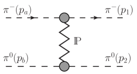
Figure 4: Diagram with pomeron exchange for $\pi^{-}\pi^{0}\to\pi^{-}\pi^{0}$ in the tensor-pomeron model.

The pomeron-exchange diagram for the reaction (2) $\pi^{-}\pi^{0}\to\pi^{-}\pi^{0}$, allowing the pions to be off-shell, is shown in Fig. 4, and easily evaluated. We get with the kinematic variables of (7) and (8) for (9):

$${\cal M}^{(0)}_{\mathbb{P}}(s_{L},t,m_{a}^{2},m_{b}^{2},m_{1}^{2},m_{2}^{2})=i{\cal F}_{\mathbb{P}}(s,t)\left[2(p_{a}+p_{1},p_{b}+p_{2})^{2}-\frac{1}{2}(p_{a}+p_{1})^{2}(p_{b}+p_{2})^{2}\right]$$

$$\qquad\qquad\qquad=i{\cal F}_{\mathbb{P}}(s,t)\left[2(2s_{L}+t)^{2}-\frac{1}{2}(-t+2m_{a}^{2}+2m_{1}^{2})(-t+2m_{b}^{2}+2m_{2}^{2})\right]\,.$$ (81)

Here we set

$${\cal F}_{\mathbb{P}}(s,t) = {\cal F}_{\mathbb{P}}\left[s_{L}+\frac{1}{2}(m_{a}^{2}+m_{b}^{2}+m_{1}^{2}+m_{2}^{2}),t\right]$$ (82)

$$= \left[2\beta_{\mathbb{P}\pi\pi}F_{M}(t)\right]^{2}\frac{1}{4s}(-is\alpha^{\prime}_{\mathbb{P}})^{\alpha_{\mathbb{P}}(t)-1}\,.$$

For the scattering of $\pi^{-}\pi^{0}\to\pi^{-}\pi^{0}$ with on-shell pions this gives

$$\left.\braket{\pi^{-}(p_{1}),\pi^{0}(p_{2})}{{\cal T}}{\pi^{-}(p_{a}),\pi^{0}(p_{b})}\right|_{\rm on\;shell}={\cal M}^{(0)}_{\mathbb{P}}(s_{L},t,m_{\pi}^{2},m_{\pi}^{2},m_{\pi}^{2},m_{\pi}^{2})$$

$$\qquad\qquad=i{\cal F}_{\mathbb{P}}(s,t)\left[2(p_{a}+p_{1},p_{b}+p_{2})^{2}-\frac{1}{2}(p_{a}+p_{1})^{2}(p_{b}+p_{2})^{2}\right]$$

$$\qquad\qquad=8is^{2}{\cal F}_{\mathbb{P}}(s,t)\Big{[}1-\frac{4m_{\pi}^{2}-t}{s}+\frac{3}{16s^{2}}(4m_{\pi}^{2}-t)^{2}\Big{]}\,,$$ (83)

$$\sigma_{\rm tot}(\pi^{-}\pi^{0})=\frac{1}{\sqrt{s(s-4m_{\pi}^{2})}}\,{\rm Im}\braket{\pi^{-}(p_{a}),\pi^{0}(p_{b})}{{\cal T}}{\pi^{-}(p_{a}),\pi^{0}(p_{b})}$$

$$\qquad=2\left(2\beta_{\mathbb{P}\pi\pi}\right)^{2}(s\alpha^{\prime}_{\mathbb{P}})^{\epsilon_{\mathbb{P}}}\cos\left(\frac{\pi}{2}\epsilon_{\mathbb{P}}\right)\Big{(}1-\frac{4m_{\pi}^{2}}{s}\Big{)}^{-1/2}\Big{[}1-\frac{4m_{\pi}^{2}}{s}+\frac{3}{16}\Big{(}\frac{4m_{\pi}^{2}}{s}\Big{)}^{2}\Big{]}\,.\quad$$ (84)

Now we come to the photon-emission process (3)

$$\pi^{-}(p_{a})+\pi^{0}(p_{b})\to\pi^{-}(p_{1}^{\prime})+\pi^{0}(p_{2}^{\prime})+\gamma(k,\epsilon)\,.$$ (85)

The relevant kinematic variables are here

$$s=(p_{a}+p_{b})^{2}=(p_{1}^{\prime}+p_{2}^{\prime}+k)^{2}\,,$$

$$t_{1}=(p_{a}-p_{1}^{\prime})^{2}=(p_{b}-p_{2}^{\prime}-k)^{2}\,,$$

$$t_{2}=(p_{b}-p_{2}^{\prime})^{2}=(p_{a}-p_{1}^{\prime}-k)^{2}\,.$$ (86)

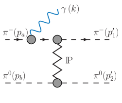
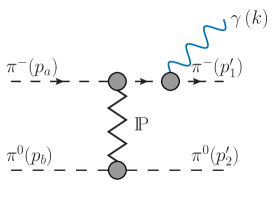
(a) (b) (c)

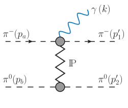
Figure 5: Pomeron-exchange diagrams for $\pi^{-}\pi^{0}\to\pi^{-}\pi^{0}\gamma$ in the tensor-pomeron model.

We have to calculate ${\cal M}_{\lambda\mathbb{P}}$ (14), (15) from the diagrams of Fig. 5. First we calculate ${\cal M}^{(a)}_{\lambda\mathbb{P}}$ and ${\cal M}^{(b)}_{\lambda\mathbb{P}}$ from (12) and (13), respectively, inserting for ${\cal M}^{(0)}$ the tensor-pomeron expression (81). Furthermore, we use the standard pion propagator and the standard $\gamma\pi\pi$ vertex function (see e.g. Ewerz:2013kda ; Bolz:2014mya ). This gives

$$\Delta[(p_{a}-k)^{2}]\,\Gamma_{\lambda}(p_{a}-k,p_{a})=\frac{(2p_{a}-k)_{\lambda}}{-2(p_{a}\cdot k)+k^{2}}\,,$$

$$\Gamma_{\lambda}(p_{1}^{\prime},p_{1}^{\prime}+k)\,\Delta[(p_{1}^{\prime}+k)^{2}]=\frac{(2p_{1}^{\prime}+k)_{\lambda}}{2(p_{1}^{\prime}\cdot k)+k^{2}}\,.$$ (87)

From (36) and (37) we see that in QFT these relations are exact for $\omega\to 0$ up to corrections of order $\omega$. For us (87) is part of our model assumptions.

With (81) and (87) we get from (12) the following amplitude ${\cal M}^{(a)}_{\lambda\mathbb{P}}$ corresponding to the diagram of Fig. 5 (a):

$${\cal M}_{\lambda\mathbb{P}}^{(a)}=-e\,{\cal M}_{\mathbb{P}}^{(0,\,a)}\,\frac{(2p_{a}-k)_{\lambda}}{-2(p_{a}\cdot k)+k^{2}}\,,$$

$${\cal M}_{\mathbb{P}}^{(0,\,a)}=i{\cal F}_{\mathbb{P}}[(p_{a}+p_{b}-k)^{2},t_{2}]\left[2(p_{a}+p_{1}^{\prime}-k,p_{b}+p_{2}^{\prime})^{2}-\frac{1}{2}(p_{a}+p_{1}^{\prime}-k)^{2}(p_{b}+p_{2}^{\prime})^{2}\right].$$

(88)

From (13) we get for ${\cal M}^{(b)}_{\lambda\mathbb{P}}$ corresponding to the diagram of Fig. 5 (b):

$${\cal M}_{\lambda\mathbb{P}}^{(b)}=-e\,\frac{(2p_{1}^{\prime}+k)_{\lambda}}{2(p_{1}^{\prime}\cdot k)+k^{2}}\,{\cal M}_{\mathbb{P}}^{(0,\,b)}\,,$$

$${\cal M}_{\mathbb{P}}^{(0,\,b)}=i{\cal F}_{\mathbb{P}}(s,t_{2})\left[2(p_{a}+p_{1}^{\prime}+k,p_{b}+p_{2}^{\prime})^{2}-\frac{1}{2}(p_{a}+p_{1}^{\prime}+k)^{2}(p_{b}+p_{2}^{\prime})^{2}\right].$$ (89)

For ${\cal M}^{(c)}_{\lambda\mathbb{P}}$ we get from (23)

$$k^{\lambda}{\cal M}_{\lambda\mathbb{P}}^{(c)} = -e{\cal M}_{\mathbb{P}}^{(0,\,a)}+e{\cal M}_{\mathbb{P}}^{(0,\,b)}$$ (90)

$$-ie\big{\{}{\cal F}_{\mathbb{P}}(s,t_{2})\big{[}-8(k,p_{b}+p_{2}^{\prime})(p_{a}+p_{1}^{\prime},p_{b}+p_{2}^{\prime})+2(k,p_{a}+p_{1}^{\prime})(p_{b}+p_{2}^{\prime})^{2}\big{]}$$

$$+\big{[}{\cal F}_{\mathbb{P}}[(p_{a}+p_{b}-k)^{2},t_{2})]-{\cal F}_{\mathbb{P}}(s,t_{2})\big{]}$$

$$\times\big{[}2(p_{a}+p_{1}^{\prime}-k,p_{b}+p_{2}^{\prime})^{2}-\frac{1}{2}(p_{a}+p_{1}^{\prime}-k)^{2}(p_{b}+p_{2}^{\prime})^{2}\big{]}\big{\}}\,.$$

Using the explicit expression for ${\cal F}_{\mathbb{P}}(s,t_{2})$ (82) we get

$${\cal F}_{\mathbb{P}}[(p_{a}+p_{b}-k)^{2},t_{2})]-{\cal F}_{\mathbb{P}}(s,t_{2})={\cal F}_{\mathbb{P}}(s,t_{2})\,\left(2-\alpha_{\mathbb{P}}(t_{2})\right)\,\frac{2(p_{a}+p_{b},k)-k^{2}}{s}\,g_{\mathbb{P}}(\varkappa,t_{2})\,,$$

(91)

where we define

$$\varkappa = \frac{2(p_{a}+p_{b},k)-k^{2}}{s}\,,$$ (92)

$$g_{\mathbb{P}}(\varkappa,t_{2}) = \frac{1}{\left(2-\alpha_{\mathbb{P}}(t_{2})\right)\varkappa}\big{[}(1-\varkappa)^{\alpha_{\mathbb{P}}(t_{2})-2}-1\big{]}$$ (93)

$$= 1+\frac{\varkappa}{2!}\left(3-\alpha_{\mathbb{P}}(t_{2})\right)+\frac{\varkappa^{2}}{3!}\left(3-\alpha_{\mathbb{P}}(t_{2})\right)\left(4-\alpha_{\mathbb{P}}(t_{2})\right)+\ldots\,.$$

The series expansion in (93) is absolutely convergent for $|\varkappa|<1$ which is the only region of interest for us.

Inserting (91) in (90) we get

$$k^{\lambda}{\cal M}^{(c)}_{\lambda\mathbb{P}} = -ie{\cal F}_{\mathbb{P}}(s,t_{2})\big{\{}-8(k,p_{b}+p_{2}^{\prime})(p_{a}+p_{1}^{\prime},p_{b}+p_{2}^{\prime})+2(k,p_{a}+p_{1}^{\prime})(p_{b}+p_{2}^{\prime})^{2}$$ (94)

$$+\frac{2(p_{a}+p_{b},k)-k^{2}}{s}\,\left(2-\alpha_{\mathbb{P}}(t_{2})\right)\,g_{\mathbb{P}}(\varkappa,t_{2})$$

$$\times\big{[}2(p_{a}+p_{1}^{\prime}-k,p_{b}+p_{2}^{\prime})^{2}-\frac{1}{2}(p_{a}+p_{1}^{\prime}-k)^{2}(p_{b}+p_{2}^{\prime})^{2}\big{]}\big{\}}\,.$$

From this we see that a simple solution of (94) for ${\cal M}^{(c)}_{\lambda\mathbb{P}}$ is

$${\cal M}^{(c)}_{\lambda\mathbb{P}} = -ie{\cal F}_{\mathbb{P}}(s,t_{2})\big{\{}-8(p_{b}+p_{2}^{\prime})_{\lambda}(p_{a}+p_{1}^{\prime},p_{b}+p_{2}^{\prime})+2(p_{a}+p_{1}^{\prime})_{\lambda}(p_{b}+p_{2}^{\prime})^{2}$$ (95)

$$+(2p_{a}+2p_{b}-k)_{\lambda}\,\left(2-\alpha_{\mathbb{P}}(t_{2})\right)\,g_{\mathbb{P}}(\varkappa,t_{2})$$

$$\times\frac{1}{s}\big{[}2(p_{a}+p_{1}^{\prime}-k,p_{b}+p_{2}^{\prime})^{2}-\frac{1}{2}(p_{a}+p_{1}^{\prime}-k)^{2}(p_{b}+p_{2}^{\prime})^{2}\big{]}\big{\}}\,.$$

However, we could add to ${\cal M}^{(c)}_{\lambda\mathbb{P}}$ from (95), for instance, terms proportional to

$$p_{a\lambda}(p_{1}^{\prime}\cdot k)-p^{\prime}_{1\lambda}(p_{a}\cdot k)\,,$$ (96)

or

$$\varepsilon_{\lambda\mu\nu\rho}p_{a}^{\mu}p_{b}^{\nu}k^{\rho}\big{(}\varepsilon_{\alpha\beta\gamma\delta}p_{a}^{\alpha}p_{b}^{\beta}p_{1}^{\prime\gamma}p_{2}^{\prime\delta}\big{)}\,,$$ (97)

and still have a solution of (94). Thus, the solution (95) for ${\cal M}^{(c)}_{\lambda\mathbb{P}}$ is in general not unique as it is to order $\omega^{0}$; see (62). This fact is well known in the literature; see for instance Bern:2014vva .

Collecting now everything together we get for the amplitude of reaction (85) in our model

$${\cal M}_{\lambda\mathbb{P}}^{(\pi^{-}\pi^{0}\to\pi^{-}\pi^{0}\gamma)}={\cal M}_{\lambda\mathbb{P}}^{(a)}+{\cal M}_{\lambda\mathbb{P}}^{(b)}+{\cal M}_{\lambda\mathbb{P}}^{(c)}$$ (98)

with ${\cal M}_{\lambda\mathbb{P}}^{(c)}$ given in (95) and ${\cal M}_{\lambda\mathbb{P}}^{(a)}$ and ${\cal M}_{\lambda\mathbb{P}}^{(b)}$ obtained from (88), (89) and (91), as follows:

$${\cal M}_{\lambda\mathbb{P}}^{(a)}=ie{\cal F}_{\mathbb{P}}(s,t_{2})\Big{[}1+\left(2-\alpha_{\mathbb{P}}(t_{2})\right)\,\frac{2(p_{a}+p_{b},k)-k^{2}}{s}\,g_{\mathbb{P}}(\varkappa,t_{2})\Big{]}$$

$$\qquad\quad\;\;\times\left[2(p_{a}+p_{1}^{\prime}-k,p_{b}+p_{2}^{\prime})^{2}-\frac{1}{2}(p_{a}+p_{1}^{\prime}-k)^{2}(p_{b}+p_{2}^{\prime})^{2}\right]\frac{(2p_{a}-k)_{\lambda}}{2(p_{a}\cdot k)-k^{2}}\,,\qquad$$ (99)

$${\cal M}_{\lambda\mathbb{P}}^{(b)}=-ie{\cal F}_{\mathbb{P}}(s,t_{2})\left[2(p_{a}+p_{1}^{\prime}+k,p_{b}+p_{2}^{\prime})^{2}-\frac{1}{2}(p_{a}+p_{1}^{\prime}+k)^{2}(p_{b}+p_{2}^{\prime})^{2}\right]\frac{(2p_{1}^{\prime}+k)_{\lambda}}{2(p_{1}^{\prime}\cdot k)+k^{2}}.$$

(100)

These results hold for arbitrary $k$. Below in Sec. V we shall consider only real photon emission where we have $k^{2}=0$.

Some comments on these results are in order. We are interested in soft photon emission where $\omega\ll\sqrt{s}$. We have then from (92) and (93) $|\varkappa|={\cal O}(\omega/\sqrt{s})$ and $g_{\mathbb{P}}(\varkappa,t_{2})\approx 1$. Looking at ${\cal M}_{\lambda\mathbb{P}}^{(a)}$ we see that there the term proportional to $g_{\mathbb{P}}(\varkappa,t_{2})$ is a correction of order $\omega/\sqrt{s}$ relative to the leading term. On the other hand, in ${\cal M}_{\lambda\mathbb{P}}^{(c)}$ the term proportional to $g_{\mathbb{P}}(\varkappa,t_{2})$ is not suppressed relative to the first term in the wavy brackets of (95). But in the soft photon region ${\cal M}_{\lambda\mathbb{P}}^{(c)}$ is, anyway, only of order $\omega/\sqrt{s}$ relative to ${\cal M}_{\lambda\mathbb{P}}^{(a)}$ and ${\cal M}_{\lambda\mathbb{P}}^{(b)}$. Thus, in the soft-photon region our model should give reliable results. But the question arises how high we can go in $\omega$ and still trust the model. We have, as basis of the model, used the high-energy approximation, given by the pomeron-exchange term, for the $\pi\pi$ scattering amplitude. Therefore, in ${\cal M}^{(0)}$ (81), (82) the c.m. energy squared $s$ should be large enough, above the resonance region, say

$$s\geqslant s_{0}=(5\;{\rm GeV})^{2}\,.$$ (101)

But in the reaction $\pi\pi\to\pi\pi\gamma$ we need the off-shell amplitudes ${\cal M}^{(0,a)}$ (88) and ${\cal M}^{(0,b)}$ (89) where the squared c.m. energies are, respectively,

$$s_{a}=(p_{a}+p_{b}-k)^{2}=(p_{1}^{\prime}+p_{2}^{\prime})^{2}\,,$$ (102)

$$s_{b}=s\,.$$ (103)

Surely, in order to apply our Regge model also for ${\cal M}^{(0,a)}$ we should require

$$s_{a}=(p_{a}+p_{b}-k)^{2}=s-2(p_{a}+p_{b},k)+k^{2}\geqslant s_{0}\,.$$ (104)

In the overall c.m. system this means

$$\omega\leqslant\frac{1}{2\sqrt{s}}\,\left(s-s_{0}+k^{2}\right)\,.$$ (105)

Below, in Sec. V, we shall take this constraint into account.

In Bolz:2014mya vertices for the coupling of $\gamma\pi\pi$ and $\mathbb{P}\gamma\pi\pi$ were derived from a Lagrangian; see (B.66)–(B.71) there. Using these vertices for evaluating the diagrams of Fig. 5 and using in all three diagrams the pomeron propagator $\Delta^{(\mathbb{P})}_{\mu\nu,\kappa\lambda}(s,t_{2})$ with the common value $s=(p_{a}+p_{b})^{2}$ gives ${\cal M}_{\lambda\mathbb{P}}^{(a)}$, ${\cal M}_{\lambda\mathbb{P}}^{(b)}$ and ${\cal M}_{\lambda\mathbb{P}}^{(c)}$ as in (99), (100), and (95), respectively, but setting $g_{\mathbb{P}}(\varkappa,t_{2})=0$. Thus, our full results for ${\cal M}_{\lambda\mathbb{P}}^{(a)}$, ${\cal M}_{\lambda\mathbb{P}}^{(b)}$, ${\cal M}_{\lambda\mathbb{P}}^{(c)}$ above are an improvement of the simple results, as we respect now the general QFT structure of the amplitudes shown in Fig. 2. As discussed above, for soft photons the improvement amounts to suitable additions of non-leading terms of relative order $\omega/\sqrt{s}$.

What about anomalous soft photons in this framework? Given the amplitude for $\pi^{-}\pi^{0}\to\pi^{-}\pi^{0}$ we have constructed ${\cal M}_{\lambda\mathbb{P}}^{(a)}$ and ${\cal M}_{\lambda\mathbb{P}}^{(b)}$ in a straightforward way. Of course, we had to extrapolate to off-shell pions and to assume (87) to hold not only for $\omega\to 0$. But by and large we think that ${\cal M}_{\lambda\mathbb{P}}^{(a)}$ and ${\cal M}_{\lambda\mathbb{P}}^{(b)}$ leave little room for anomalous soft photons. This is quite different for ${\cal M}_{\lambda\mathbb{P}}^{(c)}$ which we determined here as the simplest solution of the gauge-invariance condition (94). Clearly, other solutions of (94) for ${\cal M}_{\lambda\mathbb{P}}^{(c)}$ are possible which could describe “anomalous” production of soft photons. One of the present authors has been involved in a suggestion for the origin of such anomalous soft photons: “synchrotron radiation from the vacuum” Nachtmann:1983uz ; Botz:1994bg ; Nachtmann:ELFE ; Nachtmann:Lectures ; Nachtmann:2014qta . For a list of suggestions by other authors we refer to Wong:2014pY .

IV.2 Charged-pion scattering without and with photon radiation

In this section we consider the following reactions at high energies in the tensor-pomeron model:

$$\pi^{-}(p_{a})+\pi^{+}(p_{b})\to\pi^{-}(p_{1})+\pi^{+}(p_{2})\,,$$ (106)

$$\pi^{-}(p_{a})+\pi^{+}(p_{b})\to\pi^{-}(p_{1}^{\prime})+\pi^{+}(p_{2}^{\prime})+\gamma(k,\epsilon)\,,$$ (107)

and

$$\pi^{\pm}(p_{a})+\pi^{\pm}(p_{b})\to\pi^{\pm}(p_{1})+\pi^{\pm}(p_{2})\,,$$ (108)

$$\pi^{\pm}(p_{a})+\pi^{\pm}(p_{b})\to\pi^{\pm}(p_{1}^{\prime})+\pi^{\pm}(p_{2}^{\prime})+\gamma(k,\epsilon)\,.$$ (109)

Again we leave $k$ arbitrary and do not require $k^{2}=0$.

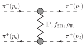
Figure 6: The diagram for $\pi^{-}\pi^{+}\to\pi^{-}\pi^{+}$ elastic scattering with exchange of the pomeron, the $f_{2\mathbb{R}}$, and the $\rho_{\mathbb{R}}$ reggeons.

The diagrams for the elastic scattering processes (106) and (108) are analogous to the one in Fig. 4 but now we include the subleading $f_{2\mathbb{R}}$ and $\rho_{\mathbb{R}}$ reggeon exchanges; see Fig. 6. To evaluate these diagrams we need the effective $f_{2\mathbb{R}}$ and $\rho_{\mathbb{R}}$ propagators and their couplings to pions. In our model these are given in (3.12)–(3.15) and (3.53), (3.54), (3.63), (3.64) of Ewerz:2013kda , respectively. The $f_{2\mathbb{R}}$ propagator and the $f_{2\mathbb{R}}\pi\pi$ couplings are as in (77)–(79) with the replacements

$$\alpha_{\mathbb{P}}(t)\to\alpha_{f_{2\mathbb{R}}}(t)=\alpha_{f_{2\mathbb{R}}}(0)+\alpha^{\prime}_{f_{2\mathbb{R}}}t\,,$$

$$\alpha_{f_{2\mathbb{R}}}(0)=0.5475\,,\quad\alpha^{\prime}_{f_{2\mathbb{R}}}=0.9\;\mbox{GeV}^{-2}\,,$$

$$2\beta_{\mathbb{P}\pi\pi}\to\frac{g_{f_{2\mathbb{R}}\pi\pi}}{2M_{0}}\,,$$

$$g_{f_{2\mathbb{R}}\pi\pi}=9.30\,,\quad M_{0}=1\;\mbox{GeV}\,.$$ (110)

For the effective $\rho_{\mathbb{R}}$ propagator and the $\rho_{\mathbb{R}}\pi\pi$ coupling we have

$$i\Delta^{(\rho_{\mathbb{R}})}_{\mu\nu}(s,t)=ig_{\mu\nu}\frac{1}{M_{-}^{2}}\,(-is\alpha^{\prime}_{\rho_{\mathbb{R}}})^{\alpha_{\rho_{\mathbb{R}}}(t)-1}\,,$$ (111)

$$\alpha_{\rho_{\mathbb{R}}}(t)=\alpha_{\rho_{\mathbb{R}}}(0)+\alpha^{\prime}_{\rho_{\mathbb{R}}}t\,,$$

$$\alpha_{\rho_{\mathbb{R}}}(0)=0.5475\,,\quad\alpha^{\prime}_{\rho_{\mathbb{R}}}=0.9\;\mbox{GeV}^{-2}\,,$$

$$M_{-}=1.41\;\mbox{GeV}\,.$$ (112)

$$i\Gamma_{\mu}^{(\rho_{\mathbb{R}}\pi^{-}\pi^{-})}(k^{\prime},k)=-i\Gamma_{\mu}^{(\rho_{\mathbb{R}}\pi^{+}\pi^{+})}(k^{\prime},k)=\frac{i}{2}\,g_{\rho_{\mathbb{R}}\pi\pi}F_{M}[(k^{\prime}-k)^{2}]\,(k^{\prime}+k)_{\mu}\,,$$

$$g_{\rho_{\mathbb{R}}\pi\pi}=15.63\,,$$ (113)

where $F_{M}(t)$ is defined in (80).

Now everything is prepared to evaluate the diagram of Fig. 6 for the general off-shell $\pi^{-}\pi^{+}$ scattering amplitude. We get [cf. (9) and (81)]

$$\left.\braket{\pi^{-}(p_{1}),\pi^{+}(p_{2})}{{\cal T}}{\pi^{-}(p_{a}),\pi^{+}(p_{b})}\right|_{\rm off\;shell} = {\cal M}^{(0)\pi^{-}\pi^{+}}(s_{L},t,m_{a}^{2},m_{b}^{2},m_{1}^{2},m_{2}^{2})$$ (114)

$$= {\cal M}^{(0)}_{\mathbb{P}}+{\cal M}^{(0)}_{f_{2\mathbb{R}}}+{\cal M}^{(0)}_{\rho_{\mathbb{R}}}\,,$$

where

$${\cal M}^{(0)}_{\mathbb{P}} = i{\cal F}_{\mathbb{P}}(s,t)\left[2(p_{a}+p_{1},p_{b}+p_{2})^{2}-\frac{1}{2}(p_{a}+p_{1})^{2}(p_{b}+p_{2})^{2}\right]$$ (115)

$$= i{\cal F}_{\mathbb{P}}(s,t)\left[2(2s_{L}+t)^{2}-\frac{1}{2}(-t+2m_{a}^{2}+2m_{1}^{2})(-t+2m_{b}^{2}+2m_{2}^{2})\right]\,,$$

$${\cal M}^{(0)}_{f_{2\mathbb{R}}} = i{\cal F}_{f_{2\mathbb{R}}}(s,t)\left[2(p_{a}+p_{1},p_{b}+p_{2})^{2}-\frac{1}{2}(p_{a}+p_{1})^{2}(p_{b}+p_{2})^{2}\right]$$ (116)

$$= i{\cal F}_{f_{2\mathbb{R}}}(s,t)\left[2(2s_{L}+t)^{2}-\frac{1}{2}(-t+2m_{a}^{2}+2m_{1}^{2})(-t+2m_{b}^{2}+2m_{2}^{2})\right]\,,$$

$${\cal M}^{(0)}_{\rho_{\mathbb{R}}} = {\cal F}_{\rho_{\mathbb{R}}}(s,t)(p_{a}+p_{1},p_{b}+p_{2})$$ (117)

$$= {\cal F}_{\rho_{\mathbb{R}}}(s,t)(2s_{L}+t)\,.$$

Here ${\cal F}_{\mathbb{P}}(s,t)$ is defined in (82) and we have set

$${\cal F}_{f_{2\mathbb{R}}}(s,t)=\left[\frac{g_{f_{2\mathbb{R}}\pi\pi}}{2M_{0}}F_{M}(t)\right]^{2}\frac{1}{4s}(-is\alpha^{\prime}_{f_{2\mathbb{R}}})^{\alpha_{f_{2\mathbb{R}}}(t)-1}\,,$$ (118)

$${\cal F}_{\rho_{\mathbb{R}}}(s,t)=\left[\frac{g_{\rho_{\mathbb{R}}\pi\pi}}{2M_{-}}F_{M}(t)\right]^{2}(-is\alpha^{\prime}_{\rho_{\mathbb{R}}})^{\alpha_{\rho_{\mathbb{R}}}(t)-1}\,.$$ (119)

For the on-shell elastic $\pi^{-}\pi^{+}$ scattering we get, setting $m_{a}^{2}=m_{b}^{2}=m_{1}^{2}=m_{2}^{2}=m_{\pi}^{2}$ in (7), (8) and (115)–(117)

$$\braket{\pi^{-}(p_{1}),\pi^{+}(p_{2})}{{\cal T}}{\pi^{-}(p_{a}),\pi^{+}(p_{b})}={\cal M}^{(0)\pi^{-}\pi^{+}}(s_{L},t,m_{\pi}^{2},m_{\pi}^{2},m_{\pi}^{2},m_{\pi}^{2})$$

$$\qquad\equiv{\cal M}^{(0)\pi^{-}\pi^{+}}(s,t)$$

$$\qquad=i\Big{[}{\cal F}_{\mathbb{P}}(s,t)+{\cal F}_{f_{2\mathbb{R}}}(s,t)\Big{]}\Big{[}2(p_{a}+p_{1},p_{b}+p_{2})^{2}-\frac{1}{2}(p_{a}+p_{1})^{2}(p_{b}+p_{2})^{2}\Big{]}$$

$$\qquad\quad+{\cal F}_{\rho_{\mathbb{R}}}(s,t)(p_{a}+p_{1},p_{b}+p_{2})$$

$$\qquad=8is^{2}\Big{[}{\cal F}_{\mathbb{P}}(s,t)+{\cal F}_{f_{2\mathbb{R}}}(s,t)\Big{]}\Big{[}1-\frac{4m_{\pi}^{2}-t}{s}+\frac{3}{16s^{2}}(4m_{\pi}^{2}-t)^{2}\Big{]}$$

$$\qquad\quad+2s{\cal F}_{\rho_{\mathbb{R}}}(s,t)\Big{[}1-\frac{4m_{\pi}^{2}-t}{2s}\Big{]}\,.$$ (120)

For brevity of notation we use in the following the notation ${\cal M}^{(0)\pi^{-}\pi^{+}}(s,t)$ for the on-shell pion-pion elastic scattering amplitude.

Turning now to the reactions (108) of like sign $\pi\pi$ scattering we get from the diagrams analogous to Fig. 6 the following for on-shell pions

$$\braket{\pi^{+}(p_{1}),\pi^{+}(p_{2})}{{\cal T}}{\pi^{+}(p_{a}),\pi^{+}(p_{b})}=\braket{\pi^{-}(p_{1}),\pi^{-}(p_{2})}{{\cal T}}{\pi^{-}(p_{a}),\pi^{-}(p_{b})}$$

$$\qquad=8is^{2}\Big{[}{\cal F}_{\mathbb{P}}(s,t)+{\cal F}_{f_{2\mathbb{R}}}(s,t)\Big{]}\Big{[}1-\frac{4m_{\pi}^{2}-t}{s}+\frac{3}{16s^{2}}(4m_{\pi}^{2}-t)^{2}\Big{]}$$

$$\qquad\quad-2s{\cal F}_{\rho_{\mathbb{R}}}(s,t)\Big{[}1-\frac{4m_{\pi}^{2}-t}{2s}\Big{]}+(p_{1}\leftrightarrow p_{2})\,.$$ (121)

The exchange $p_{1}\leftrightarrow p_{2}$ implies $t\leftrightarrow u$ where $u=-s-t+4m_{\pi}^{2}$.

The total cross sections for $\pi\pi$ scattering are obtained from the forward-scattering amplitudes using the optical theorem. In this way we get from (120) for $\pi^{-}\pi^{+}$ scattering

$$\sigma_{{\rm tot}\,,\pi^{-}\pi^{+}}(s)=\frac{1}{\sqrt{s(s-4m_{\pi}^{2})}}\,{\rm Im}\braket{\pi^{-}(p_{a}),\pi^{+}(p_{b})}{{\cal T}}{\pi^{-}(p_{a}),\pi^{+}(p_{b})}$$

$$\qquad=2\Big{(}1-\frac{4m_{\pi}^{2}}{s}\Big{)}^{-1/2}\Big{\{}\Big{[}\left(2\beta_{\mathbb{P}\pi\pi}\right)^{2}(s\alpha^{\prime}_{\mathbb{P}})^{\alpha_{\mathbb{P}}(0)-1}\cos\left(\frac{\pi}{2}(\alpha_{\mathbb{P}}(0)-1)\right)$$

$$\qquad+\left(\frac{g_{f_{2\mathbb{R}}\pi\pi}}{2M_{0}}\right)^{2}(s\alpha^{\prime}_{f_{2\mathbb{R}}})^{\alpha_{f_{2\mathbb{R}}}(0)-1}\cos\left(\frac{\pi}{2}(\alpha_{f_{2\mathbb{R}}}(0)-1)\right)\Big{]}\Big{(}1-\frac{4m_{\pi}^{2}}{s}+\frac{3m_{\pi}^{4}}{s^{2}}\Big{)}$$

$$\qquad+\left(\frac{g_{\rho_{\mathbb{R}}\pi\pi}}{2M_{-}}\right)^{2}(s\alpha^{\prime}_{\rho_{\mathbb{R}}})^{\alpha_{\rho_{\mathbb{R}}}(0)-1}\sin\left(\frac{\pi}{2}(1-\alpha_{\rho_{\mathbb{R}}}(0))\right)\Big{(}1-\frac{2m_{\pi}^{2}}{s}\Big{)}\Big{\}}\,.$$ (122)

The total cross sections for $\pi^{+}\pi^{+}$ and $\pi^{-}\pi^{-}$ scattering are obtained from (121) for $t=0$. Here for $s\gg 4m_{\pi}^{2}$ and $t=0$ the term $(p_{1}\leftrightarrow p_{2})$ is highly suppressed and, thus, very small. Neglecting the term $(p_{1}\leftrightarrow p_{2})$ for $t=0$ we get the total cross sections for $\pi^{+}\pi^{+}$ and $\pi^{-}\pi^{-}$ scattering as in (122) but with a sign change in the $\rho_{\mathbb{R}}$ term.

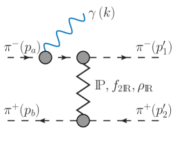
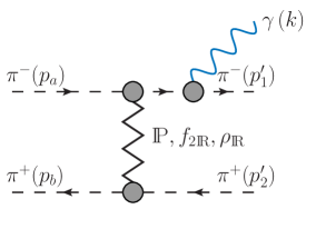
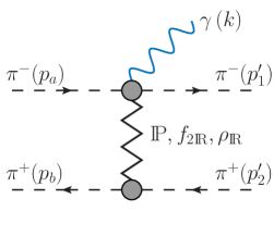
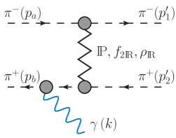
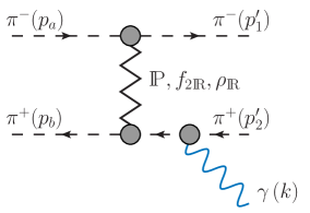
(a) (b) (c) (d) (e) (f)

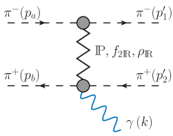
Figure 7: Diagrams for the reaction $\pi^{-}\pi^{+}\to\pi^{-}\pi^{+}\gamma$ with exchange of the pomeron, the $f_{2\mathbb{R}}$, and the $\rho_{\mathbb{R}}$ reggeons.

For the photon emission process (107) we have 6 diagrams shown in Fig. 7. The diagrams for (109) are analogous but in addition we have the diagrams with $p_{1}^{\prime}$ and $p_{2}^{\prime}$ interchanged. The kinematic variables for these reactions are as in (86). We have

$$\braket{\pi^{-}(p_{1}^{\prime}),\pi^{+}(p_{2}^{\prime}),\gamma(k,\epsilon)}{{\cal T}}{\pi^{-}(p_{a}),\pi^{+}(p_{b})}=(\epsilon^{\lambda})^{*}{\cal M}_{\lambda}^{(\pi^{-}\pi^{+}\to\pi^{-}\pi^{+}\gamma)}\,,$$ (123)

$$\braket{\pi^{+}(p_{1}^{\prime}),\pi^{+}(p_{2}^{\prime}),\gamma(k,\epsilon)}{{\cal T}}{\pi^{+}(p_{a}),\pi^{+}(p_{b})}=(\epsilon^{\lambda})^{*}{\cal M}_{\lambda}^{(\pi^{+}\pi^{+}\to\pi^{+}\pi^{+}\gamma)}\,.$$ (124)

Our building blocks for these ${\cal M}_{\lambda}$ amplitudes are ${\cal M}_{\lambda}^{(a)},\ldots,{\cal M}_{\lambda}^{(f)}$ corresponding to the diagrams (a)–(f) from Fig. 7. We have here

$${\cal M}_{\lambda}^{(a)}={\cal M}_{\lambda\mathbb{P}}^{(a)}+{\cal M}_{\lambda f_{2\mathbb{R}}}^{(a)}+{\cal M}_{\lambda\rho_{\mathbb{R}}}^{(a)}$$ (125)

and similarly for ${\cal M}_{\lambda}^{(b)},\ldots,{\cal M}_{\lambda}^{(f)}$. The amplitudes ${\cal M}_{\lambda\mathbb{P}}^{(a)}$, ${\cal M}_{\lambda\mathbb{P}}^{(b)}$, and ${\cal M}_{\lambda\mathbb{P}}^{(c)}$ are as in (99), (100), and (95), respectively. From these we obtain the amplitudes ${\cal M}_{\lambda f_{2\mathbb{R}}}^{(a)}$, ${\cal M}_{\lambda f_{2\mathbb{R}}}^{(b)}$, and ${\cal M}_{\lambda f_{2\mathbb{R}}}^{(c)}$ with the replacements (110). For $\rho_{\mathbb{R}}$ exchange we get

$${\cal M}_{\lambda\rho_{\mathbb{R}}}^{(a)} = e{\cal M}_{\rho_{\mathbb{R}}}^{(0,a)}\frac{(2p_{a}-k)_{\lambda}}{2(p_{a}\cdot k)-k^{2}}\,,$$

$${\cal M}_{\rho_{\mathbb{R}}}^{(0,a)} = {\cal F}_{\rho_{\mathbb{R}}}(s,t_{2})\Big{[}1+\left(1-\alpha_{\rho_{\mathbb{R}}}(t_{2})\right)\,\frac{2(p_{a}+p_{b},k)-k^{2}}{s}\,g_{\rho_{\mathbb{R}}}(\varkappa,t_{2})\Big{]}$$ (126)

$$\times(p_{a}+p_{1}^{\prime}-k,p_{b}+p_{2}^{\prime})\,,$$

$${\cal M}_{\lambda\rho_{\mathbb{R}}}^{(b)} = -e\frac{(2p_{1}^{\prime}+k)_{\lambda}}{2(p_{1}^{\prime}\cdot k)+k^{2}}{\cal M}_{\rho_{\mathbb{R}}}^{(0,b)}\,,$$

$${\cal M}_{\rho_{\mathbb{R}}}^{(0,b)} = {\cal F}_{\rho_{\mathbb{R}}}(s,t_{2})\,(p_{a}+p_{1}^{\prime}+k,p_{b}+p_{2}^{\prime})\,,$$ (127)

$${\cal M}_{\lambda\rho_{\mathbb{R}}}^{(c)} = e{\cal F}_{\rho_{\mathbb{R}}}(s,t_{2})\Big{\{}2(p_{b}+p_{2}^{\prime})_{\lambda}-\frac{(2p_{a}+2p_{b}-k)_{\lambda}}{s}\left(1-\alpha_{\rho_{\mathbb{R}}}(t_{2})\right)g_{\rho_{\mathbb{R}}}(\varkappa,t_{2})$$ (128)

$$\times(p_{a}+p_{1}^{\prime}-k,p_{b}+p_{2}^{\prime})\Big{\}}\,.$$

Here $\varkappa$ and $g_{\mathbb{P}}(\varkappa,t)$ are defined in (92) and (93), respectively, $g_{f_{2\mathbb{R}}}(\varkappa,t)$ is defined analogously

$$g_{f_{2\mathbb{R}}}(\varkappa,t)=\frac{1}{\left(2-\alpha_{f_{2\mathbb{R}}}(t)\right)\varkappa}\big{[}(1-\varkappa)^{\alpha_{f_{2\mathbb{R}}}(t)-2}-1\big{]}\,,$$ (129)

and $g_{\rho_{\mathbb{R}}}(\varkappa,t)$ is defined as

$$g_{\rho_{\mathbb{R}}}(\varkappa,t) = \frac{1}{\left(1-\alpha_{\rho_{\mathbb{R}}}(t)\right)\varkappa}\big{[}(1-\varkappa)^{\alpha_{\rho_{\mathbb{R}}}(t)-1}-1\big{]}\,,$$ (130)

$$= 1+\frac{\varkappa}{2!}\left(2-\alpha_{\rho_{\mathbb{R}}}(t)\right)+\frac{\varkappa^{2}}{3!}\left(2-\alpha_{\rho_{\mathbb{R}}}(t)\right)\left(3-\alpha_{\rho_{\mathbb{R}}}(t)\right)+\ldots\,.$$

We emphasize that ${\cal M}_{\lambda\mathbb{P}}^{(c)}$, ${\cal M}_{\lambda f_{2\mathbb{R}}}^{(c)}$ and ${\cal M}_{\lambda\rho_{\mathbb{R}}}^{(c)}$ are obtained as the simplest solution of the gauge-invariance relation

$$k^{\lambda}\left({\cal M}_{\lambda}^{(a)}+{\cal M}_{\lambda}^{(b)}+{\cal M}_{\lambda}^{(c)}\right)=0\,.$$ (131)

For the diagrams of Fig. 7 (d)–(f) we find

$${\cal M}_{\lambda}^{(d)}=\left.-{\cal M}_{\lambda}^{(a)}\right|_{p_{a},p_{1}^{\prime}\leftrightarrow p_{b},p_{2}^{\prime}}\,,$$ (132)

$${\cal M}_{\lambda}^{(e)}=\left.-{\cal M}_{\lambda}^{(b)}\right|_{p_{a},p_{1}^{\prime}\leftrightarrow p_{b},p_{2}^{\prime}}\,,$$ (133)

$${\cal M}_{\lambda}^{(f)}=\left.-{\cal M}_{\lambda}^{(c)}\right|_{p_{a},p_{1}^{\prime}\leftrightarrow p_{b},p_{2}^{\prime}}\,.$$ (134)

Note that $(p_{a},p_{1}^{\prime})\leftrightarrow(p_{b},p_{2}^{\prime})$ implies $t_{1}\leftrightarrow t_{2}$; see (86). We have also here

$$k^{\lambda}\left({\cal M}_{\lambda}^{(d)}+{\cal M}_{\lambda}^{(e)}+{\cal M}_{\lambda}^{(f)}\right)=0\,.$$ (135)

For the amplitudes (123) and (124) we get finally

$${\cal M}_{\lambda}^{(\pi^{-}\pi^{+}\to\pi^{-}\pi^{+}\gamma)} = {\cal M}_{\lambda}^{(a)}+{\cal M}_{\lambda}^{(b)}+{\cal M}_{\lambda}^{(c)}+{\cal M}_{\lambda}^{(d)}+{\cal M}_{\lambda}^{(e)}+{\cal M}_{\lambda}^{(f)}\,,$$ (136)

$${\cal M}_{\lambda}^{(\pi^{+}\pi^{+}\to\pi^{+}\pi^{+}\gamma)} = -\left(\hat{\cal M}_{\lambda}^{(a)}+\hat{\cal M}_{\lambda}^{(b)}+\hat{\cal M}_{\lambda}^{(c)}\right)+\hat{\cal M}_{\lambda}^{(d)}+\hat{\cal M}_{\lambda}^{(e)}+\hat{\cal M}_{\lambda}^{(f)}$$ (137)

$$+(p_{1}^{\prime}\leftrightarrow p_{2}^{\prime})\,.$$

Here we define

$$\hat{\cal M}_{\lambda}^{(a)}={\cal M}_{\lambda\mathbb{P}}^{(a)}+{\cal M}_{\lambda f_{2\mathbb{R}}}^{(a)}-{\cal M}_{\lambda\rho_{\mathbb{R}}}^{(a)}$$ (138)

and similarly for $\hat{\cal M}_{\lambda}^{(b)},\ldots,\hat{\cal M}_{\lambda}^{(f)}$.

The inclusive cross section for the real-photon yield of the reaction (107) is as follows

$$d\sigma({\pi^{-}\pi^{+}\to\pi^{-}\pi^{+}\gamma(k)})=\frac{1}{2\sqrt{s(s-4m_{\pi}^{2})}}\,\frac{d^{3}k}{(2\pi)^{3}\,2k^{0}}\int\frac{d^{3}p_{1}^{\prime}}{(2\pi)^{3}\,2p_{1}^{\prime 0}}\frac{d^{3}p_{2}^{\prime}}{(2\pi)^{3}\,2p_{2}^{\prime 0}}$$

$$\qquad\times(2\pi)^{4}\delta^{(4)}(p_{1}^{\prime}+p_{2}^{\prime}+k-p_{a}-p_{b}){\cal M}_{\lambda}^{(\pi^{-}\pi^{+}\to\pi^{-}\pi^{+}\gamma)}\big{(}{\cal M}_{\rho}^{(\pi^{-}\pi^{+}\to\pi^{-}\pi^{+}\gamma)}\big{)}^{*}(-g^{\lambda\rho})$$

(139)

and similarly for $\pi^{+}\pi^{+}\to\pi^{+}\pi^{+}\gamma$, including a statistic factor 1/2.

In the following we shall compare our “exact” model results, which we shall call “standard” results, for (136) and (137), using (99), (100), (95), (125)–(128), and (132)–(134), to various soft-photon approximations (SPAs). Below we list the explicit expressions for photon emission in $\pi^{-}\pi^{+}$ scattering.

1. Here we keep only the pole terms $\propto\omega^{-1}$ for ${\cal M}_{\lambda}^{(a)}\cdots{\cal M}_{\lambda}^{(f)}$ in (136). From (95), (99), (100), (120), (125)–(128), and (132)–(134) we see that this amounts to the following replacements, using $k^{2}=0$, and $p_{1}^{\prime}\to p_{1}$, $p_{2}^{\prime}\to p_{2}$:

   $${\cal M}_{\lambda}^{(a)}\to e{\cal M}^{(0)\pi^{-}\pi^{+}}(s,t)\frac{p_{a\lambda}}{(p_{a}\cdot k)}\,,$$

   $${\cal M}_{\lambda}^{(b)}\to-e{\cal M}^{(0)\pi^{-}\pi^{+}}(s,t)\frac{p_{1\lambda}}{(p_{1}\cdot k)}\,,$$

   $${\cal M}_{\lambda}^{(c)}\to 0\,,$$

   $${\cal M}_{\lambda}^{(d)}\to-e{\cal M}^{(0)\pi^{-}\pi^{+}}(s,t)\frac{p_{b\lambda}}{(p_{b}\cdot k)}\,,$$

   $${\cal M}_{\lambda}^{(e)}\to e{\cal M}^{(0)\pi^{-}\pi^{+}}(s,t)\frac{p_{2\lambda}}{(p_{2}\cdot k)}\,,$$

   $${\cal M}_{\lambda}^{(f)}\to 0\,.$$ (140)

   From (136) and (140) we get then

   $${\cal M}_{\lambda}^{(\pi^{-}\pi^{+}\to\pi^{-}\pi^{+}\gamma)}\to{\cal M}_{\lambda,\;{\rm SPA1}}^{(\pi^{-}\pi^{+}\to\pi^{-}\pi^{+}\gamma)}$$

   $$\qquad\qquad=e{\cal M}^{(0)\pi^{-}\pi^{+}}(s,t)\Big{[}\frac{p_{a\lambda}}{(p_{a}\cdot k)}-\frac{p_{1\lambda}}{(p_{1}\cdot k)}-\frac{p_{b\lambda}}{(p_{b}\cdot k)}+\frac{p_{2\lambda}}{(p_{2}\cdot k)}\Big{]}.$$ (141)

   Inserting this in (139) we get the following SPA1 result for the inclusive photon cross section where, for consistency, we neglect the photon momentum $k$ in the energy-momentum conserving $\delta^{(4)}(.)$ function:

   $$d\sigma({\pi^{-}\pi^{+}\to\pi^{-}\pi^{+}\gamma(k)})_{\,\rm SPA1}=\frac{d^{3}k}{(2\pi)^{3}\,2k^{0}}\int d^{3}p_{1}\,d^{3}p_{2}\,e^{2}$$

   $$\qquad\times\Big{[}\frac{p_{a\lambda}}{(p_{a}\cdot k)}-\frac{p_{1\lambda}}{(p_{1}\cdot k)}-\frac{p_{b\lambda}}{(p_{b}\cdot k)}+\frac{p_{2\lambda}}{(p_{2}\cdot k)}\Big{]}$$

   $$\qquad\times\Big{[}\frac{p_{a\rho}}{(p_{a}\cdot k)}-\frac{p_{1\rho}}{(p_{1}\cdot k)}-\frac{p_{b\rho}}{(p_{b}\cdot k)}+\frac{p_{2\rho}}{(p_{2}\cdot k)}\Big{]}(-g^{\lambda\rho})$$

   $$\qquad\times\frac{d\sigma(\pi^{-}\pi^{+}\to\pi^{-}\pi^{+})}{d^{3}p_{1}d^{3}p_{2}}\,,$$ (142)

   where

   $$\frac{d\sigma(\pi^{-}\pi^{+}\to\pi^{-}\pi^{+})}{d^{3}p_{1}d^{3}p_{2}} = \frac{1}{2\sqrt{s(s-4m_{\pi}^{2})}}\,\frac{1}{(2\pi)^{3}\,2p_{1}^{0}\,(2\pi)^{3}\,2p_{2}^{0}}$$ (143)

   $$\times(2\pi)^{4}\delta^{(4)}(p_{1}+p_{2}-p_{a}-p_{b})\,|{\cal M}^{(0)\pi^{-}\pi^{+}}(s,t)|^{2}\,.\qquad$$

   In (142), (143) we have a frequently used SPA. One takes the distribution of the particles without radiation [see (143)] and multiplies with the square of the emission factor in the square brackets in (141).

2. Here we take into account that the squared momentum transfer is $t_{2}$ for the diagrams of Fig. 7 (a)–(c) and $t_{1}$ for those of Fig. 7 (d)–(f), where $t_{1,2}$ are defined in (86). We make in (139) the replacement:

   $${\cal M}_{\lambda}^{(\pi^{-}\pi^{+}\to\pi^{-}\pi^{+}\gamma)}\to{\cal M}_{\lambda,\;{\rm SPA2}}^{(\pi^{-}\pi^{+}\to\pi^{-}\pi^{+}\gamma)}$$

   $$\qquad\qquad=e{\cal M}^{(0)\pi^{-}\pi^{+}}(s,t_{2})\Big{[}\frac{p_{a\lambda}}{(p_{a}\cdot k)}-\frac{p_{1\lambda}^{\prime}}{(p_{1}^{\prime}\cdot k)}\Big{]}$$

   $$\qquad\qquad\quad+e{\cal M}^{(0)\pi^{-}\pi^{+}}(s,t_{1})\Big{[}-\frac{p_{b\lambda}}{(p_{b}\cdot k)}+\frac{p_{2\lambda}^{\prime}}{(p_{2}^{\prime}\cdot k)}\Big{]}.$$

   (144)

   In the calculation of the photon distribution we keep the correct energy-momentum conserving $\delta^{(4)}(.)$ function in (139).

3. In our third example we make in (139) the replacement

   $${\cal M}_{\lambda}^{(\pi^{-}\pi^{+}\to\pi^{-}\pi^{+}\gamma)}\to{\cal M}_{\lambda,\;{\rm SPA3}}^{(\pi^{-}\pi^{+}\to\pi^{-}\pi^{+}\gamma)}$$

   $$\qquad\qquad=e{\cal M}^{(0)\pi^{-}\pi^{+}}(s,t^{\prime})\Big{[}\frac{p_{a\lambda}}{(p_{a}\cdot k)}-\frac{p_{1\lambda}^{\prime}}{(p_{1}^{\prime}\cdot k)}-\frac{p_{b\lambda}}{(p_{b}\cdot k)}+\frac{p_{2\lambda}^{\prime}}{(p_{2}^{\prime}\cdot k)}\Big{]},$$ (145)

   where we choose

   $$t^{\prime}={\rm min}(t_{1},t_{2})\,.$$ (146)

   Also here we keep the correct energy-momentum conserving $\delta^{(4)}(.)$ function in the evaluation of (139).

We shall also consider approximations which we shall call “improved SPA1” and “improved SPA2”, respectively. For this we consider Fig. 7. In the diagrams (a) and (d) the squared c.m. energy of the off-shell $\pi\pi\to\pi\pi$ amplitude is $s_{a}=(p_{a}+p_{b}-k)^{2}$, in the diagrams (b) and (e) it is $s=(p_{a}+p_{b})^{2}$; see (102), (103). For real photons, $k^{2}=0$, and working in the overall c.m. system we have

$$s_{a}=s-2\omega\sqrt{s}\,.$$ (147)

Now we take, as a compromise, the average value $\tilde{s}$ of $s_{a}$ and $s$,

$$\tilde{s}=s-\omega\sqrt{s}\,,$$ (148)

as squared c.m. energy of the $\pi\pi\to\pi\pi$ amplitudes. With the amplitudes ${\cal M}^{(0)\pi^{-}\pi^{+}}(\tilde{s},t)$ and ${\cal M}^{(0)\pi^{-}\pi^{+}}(\tilde{s},t_{1,2})$ in (141) and (144), respectively, we get what we call the improved SPA1 and SPA2 results. The prescription to replace $s$ by $\tilde{s}$ (148) has been advocated by Linnyk et al. Linnyk:2015tha ; Linnyk:2015rco .

V Results

Below we show our results for elastic $\pi\pi\to\pi\pi$ scattering (subsection V.1) and results for the $\pi\pi\to\pi\pi\gamma$ reaction (subsection V.2).

V.1 Comparison with the total and elastic $\pi\pi$ cross sections

Here we compare our model results with the $\pi^{-}\pi^{+}$ and $\pi^{\pm}\pi^{\pm}$ total and total elastic cross section data.

First we briefly review the experimental results for the $\pi\pi$ total and elastic cross sections. There are no direct measurements of total and elastic $\pi\pi$ cross sections at present. However, indirect data at low and intermediate $\sqrt{s}$, the pion-pion center-of-mass energy, have been extracted from reactions like $\pi^{-}p\to\pi^{+}\pi^{-}n$, $\pi^{-}\pi^{-}\Delta^{++}$ Biswas:1967mpl ; Cohen:1973yx ; Losty:1973et ; Robertson:1973tk and $\pi^{\pm}p\to\Delta^{++}X$ and $\pi^{\pm}n\to pX$ Hanlon:1976ct ; Abramowicz:1979ca . They are compared with our predictions in Fig. 8. In the left panel the experimental data are from Biswas:1967mpl ; Cohen:1973yx ; Losty:1973et ; Robertson:1973tk ; Hanlon:1976ct ; Hoogland:1977kt ; Abramowicz:1979ca while in the right panel from Srinivasan:1975tj ; Alekseeva:1982uy .

We present for the scattering of $\pi^{-}\pi^{+}$ (opposite-sign pions) and $\pi^{\pm}\pi^{\pm}$ (same-sign pions) the total (left panel) and total elastic (right panel) cross sections versus $\sqrt{s}$. The results for the single pomeron exchange ($\mathbb{P}$), for the pomeron and $f_{2\mathbb{R}}$ reggeon exchanges ($\mathbb{P}+f_{2\mathbb{R}}$), and the complete results ($\mathbb{P}+f_{2\mathbb{R}}+\rho_{\mathbb{R}}$) are shown. The corresponding theoretical expressions are given in (110)–(122). According to our model we treat the $\rho_{\mathbb{R}}$ reggeon as effective vector exchange and the pomeron and $f_{2\mathbb{R}}$ reggeon as effective tensor exchanges. Thus, in the Regge parametrization of the $\pi^{\pm}\pi^{\pm}$ cross section, the $\rho_{\mathbb{R}}$ contributes with a sign opposite to $\mathbb{P}$ and $f_{2\mathbb{R}}$.

We find good agreement with the experimental data taking into account the default values from Ewerz:2013kda for the parameters of the propagators and vertices. One has to keep in mind that for the subleading exchanges the errors of the coupling constants are quite large, in particular for the coupling $g_{\rho_{\mathbb{R}}\pi\pi}$, as was discussed in Sec. 7.1 of Ewerz:2013kda . In addition one also has to keep in mind that there should be a smooth transition from reggeon to particle exchanges when going to very low energies. Note that the same-sign-pions channels do not contain $s$ channel resonances in contrast to the opposite-sign-pions channel. Thus, our theoretical results, which include only $t$-channel exchanges, are in better agreement with the experimental data for $\sigma^{\pi^{\pm}\pi^{\pm}}$ than for $\sigma^{\pi^{-}\pi^{+}}$. Moreover, such effects as absorption corrections and multiple soft and hard exchanges, discussed in Szczurek:2001py , were not included in our calculation. Clearly, all these topics deserve careful analyses, but this goes beyond the scope of the present paper.

There are also the data of $\pi^{\pm}\pi^{-}$ total cross sections from the analysis performed in Zakharov_data . In that work, a triple reggeon model with absorption was used to extract $\sigma_{\rm tot}^{\pi^{\pm}\pi^{-}}$ from the $\pi^{\pm}p\to\Delta^{++}X$ and $\pi^{\pm}n\to pX$ processes. The authors of Zakharov_data found that the inclusion of absorptive corrections in these two reactions decreases the results by about 10$\,\%$ to 15$\,\%$. The uncertainty of these results is large and therefore we do not show these data in Fig. 8 and instead we refer to Szczurek:2001py ; Pelaez:2004ab . In Szczurek:2001py the effect of absorption corrections (double-scattering effect) on the total cross section for $\pi\pi$ scattering as a function of $\sqrt{s}$ was discussed. The $t$-dependence of the elastic $\pi\pi$ cross sections was also discussed there. The authors of Szczurek:2001py found that the absorption is much weaker for the same-sign pions than for the opposite-sign pions; see, e.g., Figs. 5, 9 and Table 2 of Szczurek:2001py .

The total $\pi^{+}\pi^{-}$ and $\pi^{\pm}\pi^{\pm}$ cross sections including subleading reggeon exchanges were also discussed in Pelaez:2003ky ; Halzen:2011xc ; Caprini:2011ky . There is the question of the reliability of the Regge model down to low energies and whether in the region of low $\sqrt{s}$ but not low $|t|$ the Regge parametrization can be properly applied. On general grounds, one expects Regge theory to work when $s\gg|t|$, $s_{0}$ [see (101)] and $|t|\lesssim 1$ GeV² and, in fact, the Regge parametrization for $\pi\pi$ becomes unreliable at large $|t|$. The interested reader may consult Refs. Pelaez:2003ky ; Caprini:2011ky for the detailed discussion of this and other related issues.

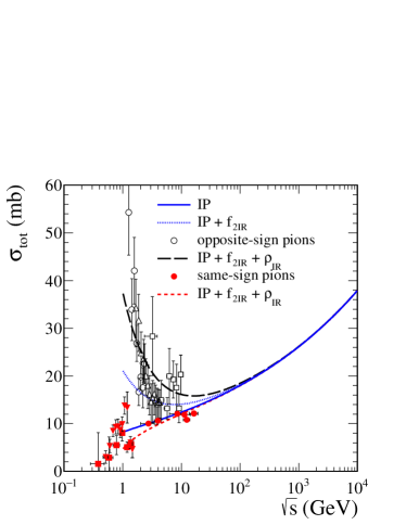
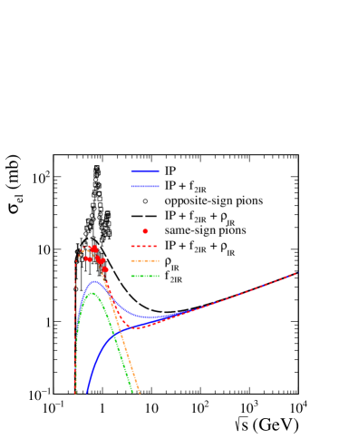
Figure 8: Results for $\pi^{-}\pi^{+}$ and $\pi^{+}\pi^{+}$ or $\pi^{-}\pi^{-}$ total (left panel) and total elastic (right panel) cross sections as a function of $\sqrt{s}$ together with the experimental data. The single pomeron exchange is given by the blue solid line, the pomeron plus $f_{2\mathbb{R}}$ reggeon exchanges by the blue dotted line, the complete result ($\mathbb{P}+f_{2\mathbb{R}}+\rho_{\mathbb{R}}$) for the opposite-sign pions and the same-sign pions is given by the black long-dashed line and the red short-dashed line, respectively. In the right panel we show also the $f_{2\mathbb{R}}$ reggeon and the $\rho_{\mathbb{R}}$ reggeon terms separately.

In the next subsection we shall discuss soft-photon emission in $\pi\pi$ scattering for c.m. energies $\sqrt{s}=10$ GeV and 100 GeV. We see from Fig. 8 that at $\sqrt{s}\gtrsim 100$ GeV the $\pi\pi$ cross sections are completely dominated by the pomeron-exchange contribution. At least, this is the result of our model. Therefore, in Sec. V.2 we shall take into account only the pomeron-exchange term for the reactions $\pi\pi\to\pi\pi\gamma$ at $\sqrt{s}\geqslant 100$ GeV. At $\sqrt{s}\simeq 10$ GeV we will show results including the pomeron exchange alone and in addition the $\rho_{\mathbb{R}}$ and $f_{2\mathbb{R}}$ reggeon exchanges. As we will show below in Fig. 14, the secondary reggeon exchanges play a significant role there.

V.2 Comparison of our “exact” model or “standard” results for the $\pi\pi\to\pi\pi\gamma$ reactions with various soft-photon approximations

First, in Fig. 9, we present the two-dimensional distributions in ($\omega$, $k_{\perp}$), ($\omega$, $\rm{y}$), and ($k_{\perp}$, $\rm{y}$), for the $\pi^{-}\pi^{+}\to\pi^{-}\pi^{+}\gamma$ reaction for our “standard” result (136), (139), including only the pomeron exchange. Calculations were done for the pion-pion collision energy $\sqrt{s}=10$ GeV. Here, $\omega=k^{0}$ is the center-of-mass photon energy, $k_{\perp}$ is the absolute value of the photon transverse momentum, and $\rm{y}$ is the rapidity of the photon. We must remember here, that in order to stay with all amplitudes in the Regge regime we certainly have to require (105) which reads here, with $k^{2}=0$ and $s_{0}=25\;{\rm GeV}^{2}$,

$$\omega\leqslant\frac{1}{2\sqrt{s}}\,\left(s-s_{0}\right)=3.75\;{\rm GeV}\,.$$ (149)

To be on the safe side, we shall in the following only show results for $\omega<3$ GeV. In the panel (a) we show the lines corresponding to the absolute value of the rapidity of the photon ${\rm y}=1,2,\ldots,6$. Large ${\rm y}$ is near the $\omega$ axis and ${\rm y}=0$ on the $k_{\perp}$ axis. There are in all three plots also regions that are not accessible kinematically. From the panel (b) we see that an upper cut on $\omega$ is effecting the upper limit of the allowed ${\rm y}$ range.

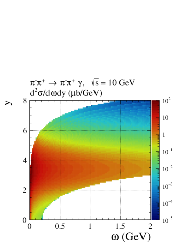
(a)
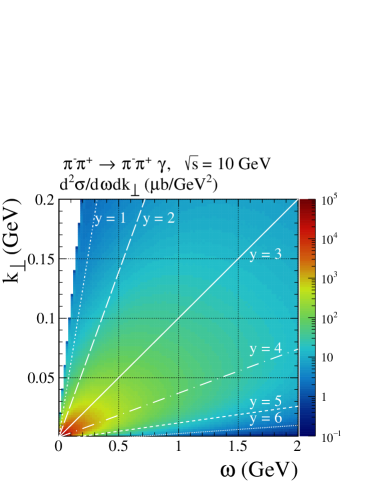
(b) (c)

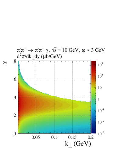
Figure 9: The two-dimensional distributions in ($\omega$, $k_{\perp}$), ($\omega$, $\rm{y}$), and ($k_{\perp}$, $\rm{y}$), for the $\pi^{-}\pi^{+}\to\pi^{-}\pi^{+}\gamma$ reaction including only the pomeron exchange. Calculations were done for $\sqrt{s}=10$ GeV, $0.001\;{\rm GeV}<k_{\perp}<0.2\;{\rm GeV}$, $\omega<3\;{\rm GeV}$, and $|\rm{y}|<8$. The lines plotted in the panel (a) correspond to the photon rapidities ${\rm y}=1,2,\ldots,6$. In panels (b) and (c) we show the results only for $0<\rm{y}<8$ since these distributions are symmetric under $\rm{y}\to-\rm{y}$.

Now we compare our “exact” model or “standard” result for the $\pi^{-}\pi^{+}\to\pi^{-}\pi^{+}\gamma$ reaction to various soft-photon approximations (SPAs) discussed in Sec. IV.2. We consider $\sqrt{s}=10$ GeV and include only the pomeron exchange.

A quantity of great interest is the ratio of the cross section calculated in one of the SPAs to the “standard” result. This ratio will now be studied as a function of $\omega=k^{0}$ and $k_{\perp}$ in the $\omega$-$k_{\perp}$ plane. In Fig. 10 we show, in two-dimensional plots, the ratio

$${\rm R}(\omega,k_{\perp})=\frac{d^{2}\sigma_{\rm SPA}/d\omega dk_{\perp}}{d^{2}\sigma_{\rm standard}/d\omega dk_{\perp}}\,.$$ (150)

The results for the three scenarios of the SPA amplitudes are presented. The result on the panels (a) corresponds to SPA1 (141), the result on the panels (b) corresponds to SPA2 (144), and the result on the panels (c) corresponds to SPA3 (145). We also show the lines corresponding to ${\rm y}=1,2,\ldots,6$.

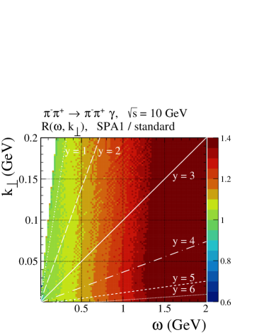
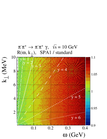
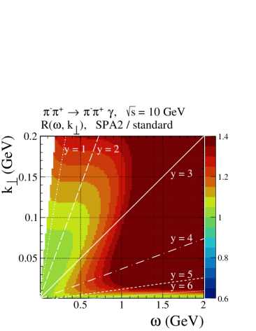
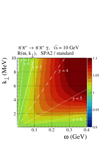
(a) (b) (c)

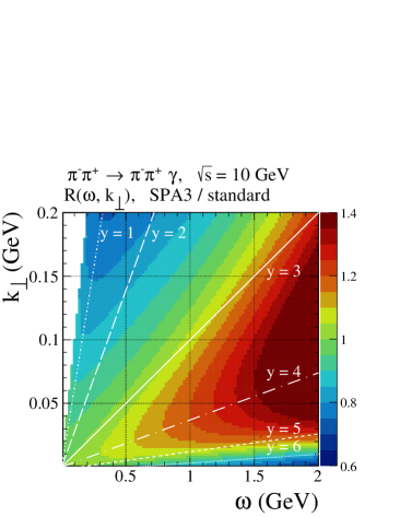
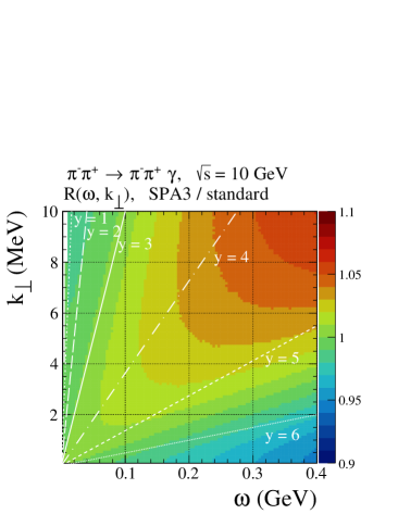
Figure 10: The ratios ${\rm R}(\omega,k_{\perp})$ (150) for the $\pi^{-}\pi^{+}\to\pi^{-}\pi^{+}\gamma$ reaction for $\sqrt{s}=10$ GeV for the three soft-photon approximations SPA1 (141), SPA2 (144), and SPA3 (145). The lines corresponding to the photon rapidities ${\rm y}=1,2,\ldots,6$ are also plotted. The right panels show the region of small $k_{\perp}$ and small $\omega$ in greater detail.

Now we discuss results separately for the three $k_{\perp}$ intervals of photon transverse momenta: $0.1\;{\rm MeV}<k_{\perp}<1\;{\rm MeV}$, $1\;{\rm MeV}<k_{\perp}<10\;{\rm MeV}$, $10\;{\rm MeV}<k_{\perp}<100\;{\rm MeV}$. We do so due to difficulties in the numerical evaluation of integrals. In Fig. 11 we show the distributions in ${\rm y}$ for the standard results [see Eq. (136)] including only the pomeron exchange. Calculations were done for $\sqrt{s}=10$ GeV and 100 GeV. When going from $\sqrt{s}=10$ GeV to $\sqrt{s}=100$ GeV the maximum of the ${\rm y}$ distribution shifts from ${\rm y_{max}}\simeq 3.4$ to ${\rm y_{max}}\simeq 5.8$.

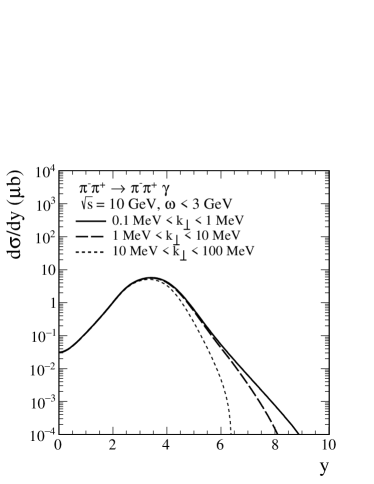
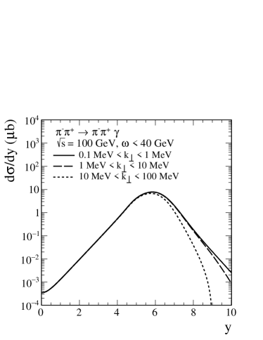
Figure 11: The distributions in rapidity of the photon in the $\pi^{-}\pi^{+}\to\pi^{-}\pi^{+}\gamma$ reaction calculated for $\sqrt{s}=10$ GeV, $\omega<3$ GeV (left panel) and for $\sqrt{s}=100$ GeV, $\omega<40$ GeV (right panel) for different $k_{\perp}$ intervals. Plotted are the results only for positive $\rm{y}$ since the distributions are symmetric under $\rm{y}\to-\rm{y}$.

In Fig. 12 we present the distributions in $k_{\perp}$ and $\omega$ for the reaction $\pi^{-}\pi^{+}\to\pi^{-}\pi^{+}\gamma$ calculated for $\sqrt{s}=10$ GeV including only the pomeron exchange. Results are shown for three $k_{\perp}$ intervals for our model and for the various SPAs. From the semi-logarithmic plots of Fig. 12 we see that the three SPAs follow the general trend of our standard results quite well for $k_{\perp}\lesssim 20$ MeV and for $\omega\lesssim 1$ GeV. But let us now have a closer look at these kinematic regions at a linear scale.

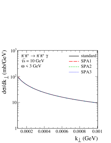
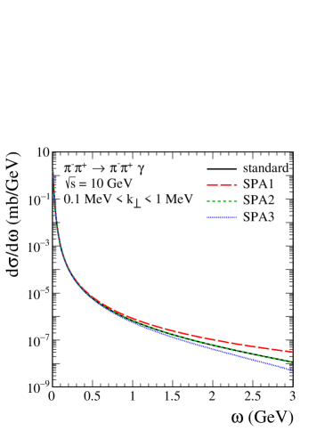
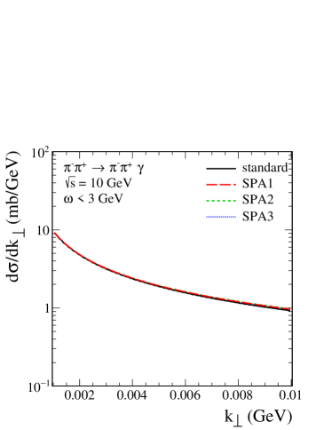
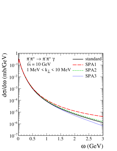
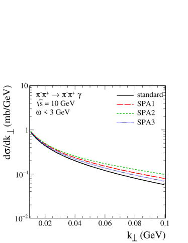
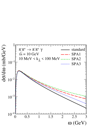
Figure 12: The differential distributions in transverse momentum of the photon and in the energy of the photon for the $\pi^{-}\pi^{+}\to\pi^{-}\pi^{+}\gamma$ reaction. The calculations were done for $\sqrt{s}=10$ GeV and $\omega<3$ GeV. The black solid line corresponds to the standard result, the red long-dashed line corresponds to SPA1 (141), the green dashed line corresponds to SPA2 (144), and the blue dotted line corresponds to SPA3 (145).

Figure 13 shows the ratios of the SPAs to the standard cross section:

$$\frac{d\sigma_{\rm SPA}/dk_{\perp}}{d\sigma_{\rm standard}/dk_{\perp}}\,\,,$$ (151)

$$\frac{d\sigma_{\rm SPA}/d\omega}{d\sigma_{\rm standard}/d\omega}\,,$$ (152)

as functions of $k_{\perp}$ and $\omega$, respectively. The rapid fluctuations of the ratio as a function of $k_{\perp}$ are due to different organization of integration in the two codes: one for the full three-body phase space (standard approach, SPA2, SPA3) and one for the two-body phase space supplemented by additional integration over photon three momentum (SPA1). The SPAs which we consider deviate from the standard results only at the percent level for $0.1\;{\rm MeV}<k_{\perp}<1\;{\rm MeV}$ but at the 10$\,\%$ to 50$\,\%$ level for $k_{\perp}\cong 50$ MeV; see the left panels of Fig. 13. From the right panels of Fig. 13 we see that the deviations of the SPAs from the standard results are up to around 50$\,\%$ for $\omega<1.5$ GeV. We also note that the discrepancies of the SPAs to the standard results typically increase rapidly with growing $k_{\perp}$ and $\omega$. For the SPA1 approximation we have on purpose set $k=0$ in the energy-momentum conserving delta function in (139), since this corresponds to a frequently used procedure in the literature. Thus, the SPA1 approach does not respect the upper kinematic limit for $\omega$. But this is no problem for us since we are interested here only in soft-photon production. But we note that the accuracy of the SPA1 can be significantly improved and the region of its applicability can be extended by keeping the correct energy-momentum conservation as in the SPA2 and SPA3.

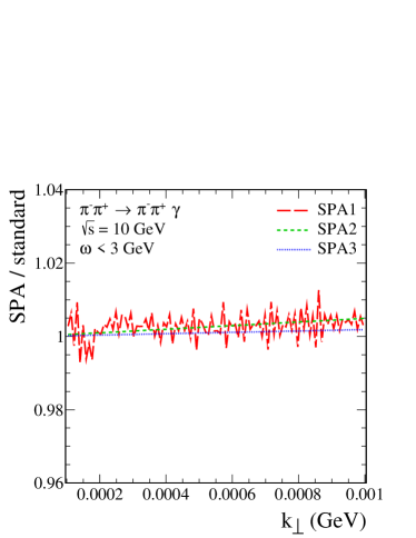
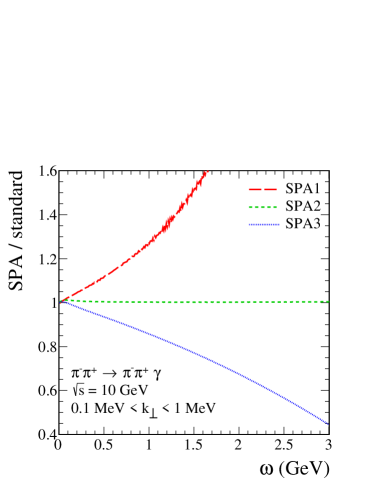
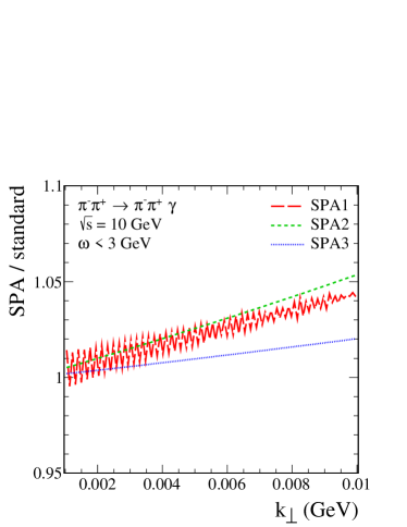
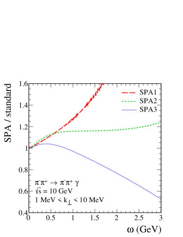
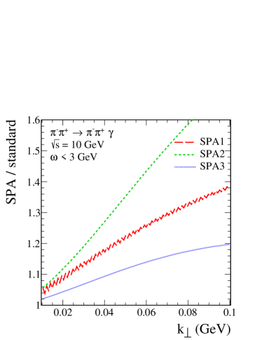
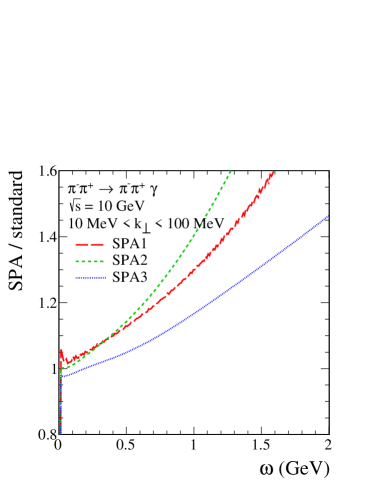
Figure 13: The ratios $\sigma_{\rm SPA}/\sigma_{\rm standard}$ given by (151) and (152), respectively. The oscillations in the SPA1 results are of numerical origin.

Now we wish to illustrate the effect of inclusion of reggeon exchanges ($\rho_{\mathbb{R}}$ and $f_{2\mathbb{R}}$) in addition to the pomeron exchange. In Fig. 14 we show the ratio $\sigma_{\rm standard}^{(\mathbb{P}+\mathbb{R})}/\sigma_{\rm standard}^{(\mathbb{P})}$ for our model as a function of $k_{\perp}$, $\omega$, and $\rm{y}$. Inclusion of the subleading reggeon exchanges in the calculations leads to a sizable increase of the cross section. We get for the ratio of the total cross sections with the cuts $1\;{\rm MeV}<k_{\perp}<10\;{\rm MeV}$ and $\omega<3$ GeV

$$\frac{\sigma_{\rm standard}^{(\mathbb{P}+\mathbb{R})}}{\sigma_{\rm standard}^{(\mathbb{P})}}=\frac{29.50\;\mu{\rm b}}{21.76\;\mu{\rm b}}\simeq 1.36\,,$$ (153)

that is, an about 36$\,\%$ increase due to the reggeon exchanges. From the ratios of differential distributions in $\omega$ and in $\rm{y}$ we see that these ratios vary from 1.25 to 1.55 depending on kinematics.

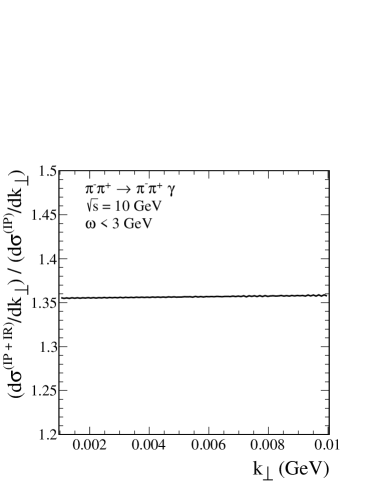
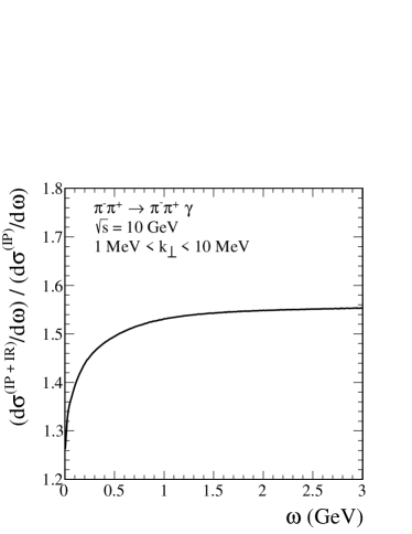
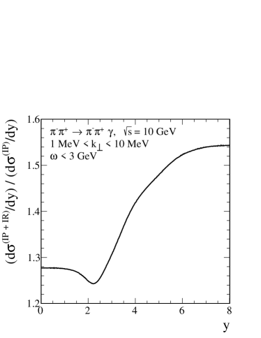
Figure 14: The ratios $\sigma_{\rm standard}^{(\mathbb{P}+\mathbb{R})}/\sigma_{\rm standard}^{(\mathbb{P})}$ in the $\pi^{-}\pi^{+}\to\pi^{-}\pi^{+}\gamma$ reaction calculated for $\sqrt{s}=10$ GeV, $1\;{\rm MeV}<k_{\perp}<10\;{\rm MeV}$, and $\omega<3$ GeV.

Now we turn to the results at c.m. energy $\sqrt{s}=100$ GeV. Here we include in the calculations only the pomeron-exchange contributions. As we see already from Fig. 8 the nonleading exchanges are negligible there.

In Fig. 15 we show the distributions in ($\omega$, $k_{\perp}$), ($\omega$, $\rm{y}$), and ($k_{\perp}$, $\rm{y}$), for our standard results. Here we consider only c.m. photon energies $\omega<10$ GeV. The constraint (105), setting $k^{2}=0$, is then always well satisfied. That is, we are in the Regge regime for all relevant amplitudes. These distributions are the analogs of those shown in Fig. 9 for $\sqrt{s}=10$ GeV.

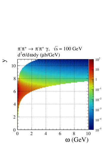
(a)
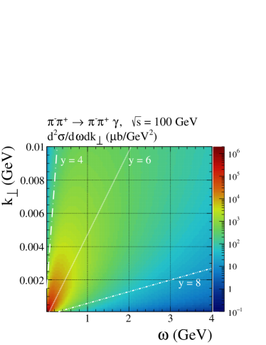
(b) (c)

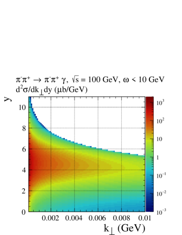
Figure 15: The two-dimensional distributions in ($\omega$, $k_{\perp}$), ($\omega$, $\rm{y}$), and ($k_{\perp}$, $\rm{y}$), for the reaction $\pi^{-}\pi^{+}\to\pi^{-}\pi^{+}\gamma$ at $\sqrt{s}=100$ GeV. This is the same as in Fig. 9 but for $\sqrt{s}=100$ GeV, $\omega<10$ GeV, and $|\rm{y}|<11$. The lines plotted in the panel (a) correspond to the photon rapidities ${\rm y}=4,6,8$.

Figure 16 shows the ratios ${\rm R}(\omega,k_{\perp})$ (150) for the reaction $\pi^{-}\pi^{+}\to\pi^{-}\pi^{+}\gamma$ at $\sqrt{s}=100$ GeV for the approximations SPA1 (141), SPA2 (144) and SPA3 (145).

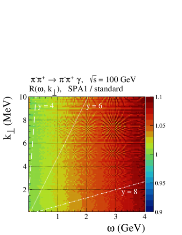
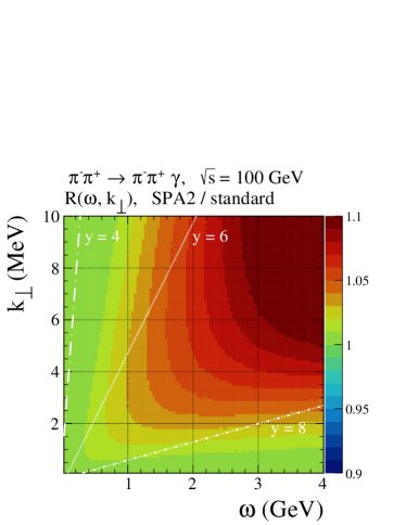
(a) (b) (c)

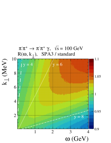
Figure 16: The ratios ${\rm R}(\omega,k_{\perp})$ (150) for the $\pi^{-}\pi^{+}\to\pi^{-}\pi^{+}\gamma$ reaction for $\sqrt{s}=100$ GeV for the three SPAs. The lines corresponding to the photon rapidities ${\rm y}=4,6,8$ are also plotted.

In Figs. 17 and 18 we show the results for $\sqrt{s}=100$ GeV which are analogs of those shown in Figs. 12 and 13 for $\sqrt{s}=10$ GeV. The calculations were done with cuts on $\omega$ specified in the figure legends. In all cases the constraint on $\omega$ from (105) is well satisfied. We see that at $\sqrt{s}=100$ GeV the three SPAs are all close to our standard results in the region of small $k_{\perp}$ and $\omega$. For $0.1\;{\rm MeV}<k_{\perp}<1\;{\rm MeV}$ the SPA1 result deviates strongly from the standard result for $\omega\gtrsim 4$ GeV; see the upper most right panel of Fig. 17. This is due to the incorrect energy-momentum $\delta$ function used, on purpose, there; see (140)–(143). Figure 18 shows that for $k_{\perp}\lesssim 10\;{\rm MeV}$ the deviations of the SPAs from the standard results are only at the percent level. For the $\omega$ distributions these differences are up to around 10$\,\%$ for $\omega\lesssim 3$ GeV.

We also note that in Fig. 18 the SPA results are in most cases above the standard results (ratio > 1) but in some cases also below (ratio < 1). Thus, the ratios SPA/standard depend strongly on the kinematics.

As for $\sqrt{s}=10$ GeV, the rapid oscillations of the ratios for SPA1 in Fig. 18 are a numerical artefact caused by different integration procedures in two different codes.

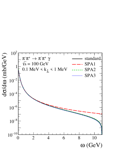
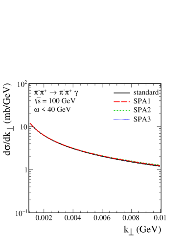
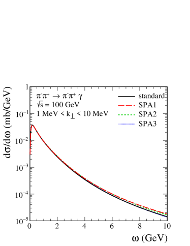
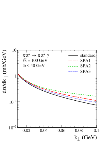
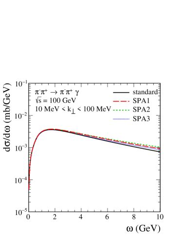
Figure 17: The same as in Fig. 12 but for $\sqrt{s}=100$ GeV. Shown are results for three $k_{\perp}$ intervals and with cuts on $\omega$ specified in the figure legends.

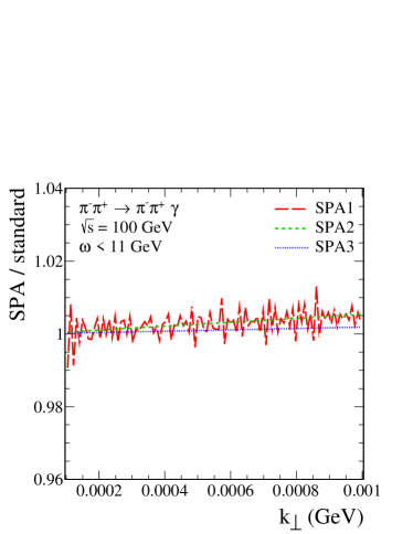
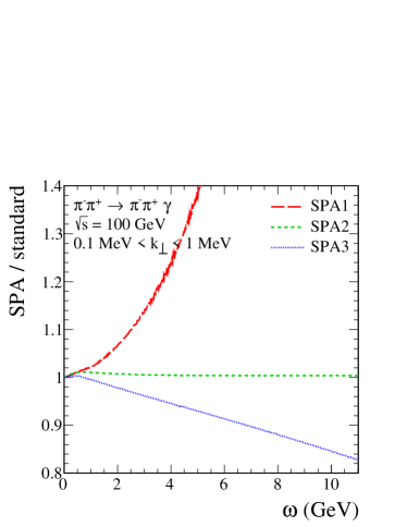
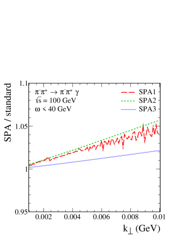
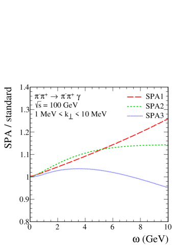
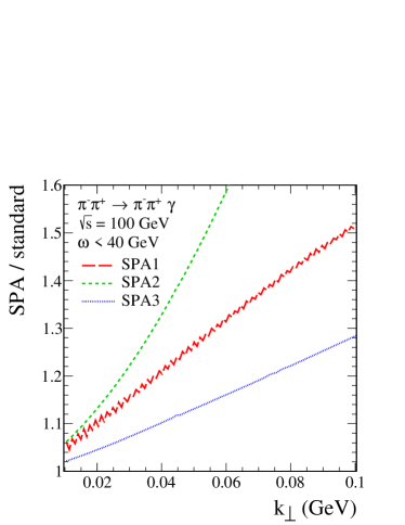
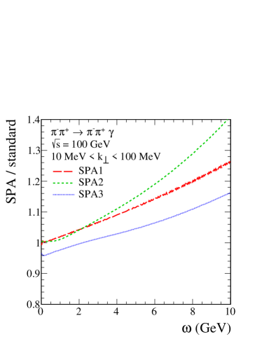
Figure 18: The same as in Fig. 13 but for $\sqrt{s}=100$ GeV. Shown are results for three $k_{\perp}$ intervals and with cuts on $\omega$ specified in the figure legends. The oscillations in the SPA1 results are of numerical origin.

At this point we can discuss the qualitative accuracy estimates of the SPA1 approximation as given a long time ago in Gribov:1966hs . For the scattering reaction this estimate is given following Eq. (19) of Gribov:1966hs and reads for our case

$$p_{a}\cdot k\approx p_{1}\cdot k\ll m_{\pi}^{2}\,,$$ (154)

$$p_{b}\cdot k\approx p_{2}\cdot k\ll m_{\pi}^{2}\,.$$ (155)

In the c.m. system, choosing $p_{a}$ in $z$ direction, $p_{a}\cdot k$ ($p_{b}\cdot k$) can only become small for the longitudinal component $k_{L}$ of $k$ being positive (negative). We have then

$$p_{a}\cdot k=p_{a}^{0}\omega-|\mbox{\boldmath$p_{a}$}|k_{L} = p_{a}^{0}\omega-|\mbox{\boldmath$p_{a}$}|\sqrt{\omega^{2}-k_{\perp}^{2}}$$ (156)

$$= \frac{2m_{\pi}^{2}\omega^{2}+\frac{1}{2}(s-4m_{\pi}^{2})\,k_{\perp}^{2}}{\sqrt{s}\omega+\sqrt{s-4m_{\pi}^{2}}\sqrt{\omega^{2}-k_{\perp}^{2}}}\quad{\rm for}\;k_{L}>0\,,$$

and

$$p_{b}\cdot k=\frac{2m_{\pi}^{2}\omega^{2}+\frac{1}{2}(s-4m_{\pi}^{2})\,k_{\perp}^{2}}{\sqrt{s}\omega+\sqrt{s-4m_{\pi}^{2}}\sqrt{\omega^{2}-k_{\perp}^{2}}}\quad{\rm for}\;k_{L}<0\,.$$ (157)

In Fig. 19 we show again the ratio SPA1/standard in the $\omega$-$k_{\perp}$ plane together with the lines

$$\frac{2m_{\pi}^{2}\omega^{2}+\frac{1}{2}(s-4m_{\pi}^{2})\,k_{\perp}^{2}}{\sqrt{s}\omega+\sqrt{s-4m_{\pi}^{2}}\sqrt{\omega^{2}-k_{\perp}^{2}}}=c\,m_{\pi}^{2}\,,\quad c=1.0,\;0.5,\;0.1,\;0.01\,.$$ (158)

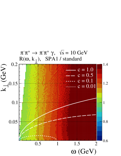
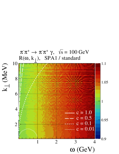
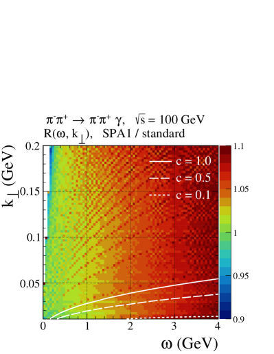
Figure 19: The ratio SPA1/standard (150) for $\sqrt{s}=10$ GeV (top panel) and for $\sqrt{s}=100$ GeV (bottom panels). The lines corresponding to $c=1.0,0.5,0.1$, and 0.01 in (158) are plotted. All other curves in the bottom right panel are numerical artefacts.

If the accuracy estimate (154), (155) would be valid, say with $p_{a}\cdot k\leqslant cm_{\pi}^{2}$ and $p_{b}\cdot k\leqslant cm_{\pi}^{2}$ and $c=0.1$ or 0.01, the area below the corresponding curves in Fig. 19 should be coloured green, indicating that there the SPA1 is a good representation of our standard result. But we see from Fig. 19 that the green areas, which we obtained from explicit calculations, seem to have only very little to do with the qualitative conditions (154), (155). The areas below the curves of constant $c$ have regions where the SPA1 is not a good representation of the standard results. On the other hand, there are large green areas above these curves where the SPA1 gives a good representation of the standard results. Of course, all these statements refer to a comparison of SPA1 to our standard results and things could be different for possible other calculations including, for instance, “anomalous” terms.

Figure 20 shows the ratios ${\rm R}(\omega,k_{\perp})$ for the two “improved SPA” scenarios calculated for $\sqrt{s}=10$ GeV and 100 GeV. Comparing these results to the corresponding results from Figs. 10 and 16 we observe that the “improved SPAs” greatly reduce the discrepancies to our standard results. This is particularly the case for the improved SPA1 case. One can see from Figs. 20 (a) and (e) that the improved SPA1 is a good approximation with the accuracy up to 10$\,\%$ for $k_{\perp}\lesssim 0.2$ GeV and $\omega\lesssim 2$ GeV for $\sqrt{s}=10$ GeV, and for $k_{\perp}\lesssim 0.2$ GeV and $\omega\lesssim 20$ GeV for $\sqrt{s}=100$ GeV.

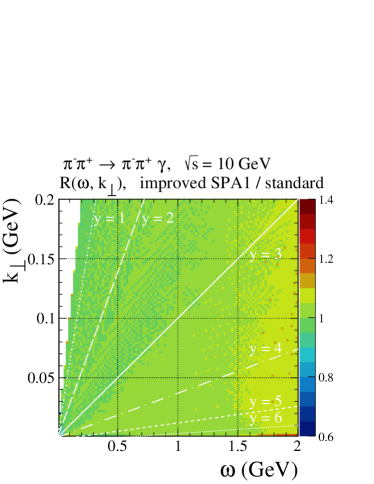
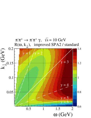
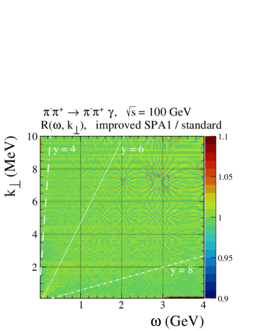
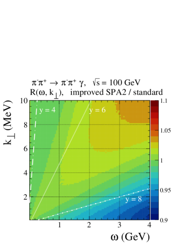
(a) (b) (c) (d) (e)

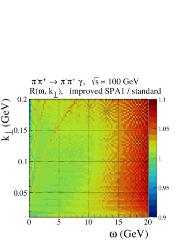
Figure 20: The ratios ${\rm R}(\omega,k_{\perp})$ (150) for the $\pi^{-}\pi^{+}\to\pi^{-}\pi^{+}\gamma$ reaction for our “improved SPA” scenarios for $\sqrt{s}=10$ GeV and 100 GeV.

VI Conclusions

In this paper we have studied elastic pion-pion scattering without and with photon radiation. In Sec. II we have given a detailed analysis, from a QFT point of view, of the reactions $\pi^{-}\pi^{0}\to\pi^{-}\pi^{0}$ and $\pi^{-}\pi^{0}\to\pi^{-}\pi^{0}\gamma$. We have used this analysis in Sec. III to derive the expansion of the amplitude for $\pi^{-}\pi^{0}\to\pi^{-}\pi^{0}\gamma$ in powers of $\omega$, the photon energy in the overall c.m. system, for $\omega\to 0$. The term of order $\omega^{-1}$ agrees with that given by F.E. Low in Low:1958sn but, to our great surprise, our term of order $\omega^{0}$ disagrees with that given in Low:1958sn . We have analysed this important discrepancy and we have shown that our expansion is for the photon-emission amplitude satisfying energy-momentum conservation. In contrast, we find that the term of order $\omega^{0}$ from Low:1958sn corresponds to the expansion of an amplitude violating energy-momentum conservation for photon-momentum $k\neq 0$. In Appendix A we compare our findings for this term of order $\omega^{0}$ to further results from the literature. We find that our result is new compared to the results of the papers which we study in Appendix A. We emphasize that our result for the $\omega^{0}$ term is a strict consequence of QFT. Therefore, absolutely no model dependence is contained there.

In Sec. IV we have calculated the amplitudes for $\pi\pi\to\pi\pi$ and $\pi\pi\to\pi\pi\gamma$ in the tensor-pomeron model. The diagrams for the latter process where the photon is emitted from the external pion lines [Fig. 7 (a), (b), (d), (e)] are determined completely by the (off-shell) $\pi\pi\to\pi\pi$ scattering amplitude. The amplitudes corresponding to the diagrams of Fig. 7 (c) and Fig. 7 (f), the “structure terms”, have to satisfy gauge-invariance constraints involving the previous amplitudes. We have given a solution of these constraints which involves again only the (off-shell) $\pi\pi\to\pi\pi$ scattering amplitude. But we have emphasized that this solution is not unique (as is well known in the literature, see e.g. Bern:2014vva ) and there “anomalous” terms in the $\pi\pi\to\pi\pi\gamma$ amplitudes, not directly related to the $\pi\pi\to\pi\pi$ amplitude, could come up. We considered then as “standard”, or “exact” model, our $\pi\pi\to\pi\pi\gamma$ amplitudes without such “anomalous” terms. Clearly, in Sec. IV we used a model. We summarize here our main model assumptions.

1. We used the tensor-pomeron model, both for the on-shell and off-shell $\pi\pi\to\pi\pi$ amplitudes. For the high-energy reactions which are our main interest we needed the effective pomeron propagator and the ${\rm pomeron}\,\pi\pi$ vertex. These quantities were taken from Ewerz:2013kda where they were derived from comparison of theory to data, in particular for nucleon-(anti)nucleon and pion-nucleon scattering.

2. We used the standard pion propagator and $\gamma\pi\pi$ vertex; see (87). Possible off-shell form factors in the pomeron- and photon-pion vertices and the pion propagator are set to one.

3. To determine the structure terms [Figs. 5 (c), 7 (c), 7 (f)] we used the simplest solutions of the respective gauge-invariance relations; see (94), (95), (128). Throughout our paper we denote as “anomalous” terms possible additional structure terms, which then have to satisfy the gauge-invariance relations by themselves. In our model we excluded such “anomalous” terms in the radiative amplitudes.

   We consider point (3) as our main model assumption.

We have defined three soft-photon approximations to our above “exact model”: SPA1, SPA2, and SPA3; see Sec. IV.2. In the SPA1 the photon momentum $k$ was, on purpose, omitted in the energy-momentum conserving $\delta^{(4)}(.)$ function in the evaluation of the cross section. In the SPA2 and SPA3 the correct energy-momentum conservation was required.

In Sec. V we have presented quantitative calculations for the elastic $\pi\pi$ scattering without and with photon radiation within the tensor-pomeron model. We have shown results for our “standard model” and for the three SPAs for two different collision energies $\sqrt{s}=10$ GeV and 100 GeV. We have shown, for instance, the results of our model for the two-dimensional distributions in photon transverse momentum $k_{\perp}$ and rapidity ${\rm y}$ [Figs. 9 (c) and 15 (c)]. For $\sqrt{s}=10$ GeV the distribution is largest for $k_{\perp}\lesssim 0.1$ GeV and $2\lesssim{\rm y}\lesssim 5$. For $\sqrt{s}=100$ GeV the distribution is largest for $k_{\perp}\lesssim 0.004$ GeV and $3\lesssim{\rm y}\lesssim 7$. These are the results of our calculations in the framework of our “standard” model where we have listed the assumptions in (1), (2), (3) above. We note that the distributions in $k_{\perp}$ and ${\rm y}$ give very small values for ${\rm y}\approx 0$, that is, in the mid-rapidity region. Clearly, this is then a region where “anomalous” contributions to the radiative amplitude could be large compared to our “standard”. But we note that such anomalous contributions cannot come directly from the high-energy exchange object, the pomeron $\mathbb{P}$. Charge-conjugation ($C$) invariance of the strong and electromagnetic interactions forbids a $\mathbb{P}\mathbb{P}\gamma$ vertex. The pomeron has $C=+1$ and the photon $C=-1$. But in $\pi\pi$ scattering there can be central exclusive production (CEP) of single photons by the fusion reactions $\mathbb{P}+\rho_{\mathbb{R}}\to\gamma$ and $f_{2\mathbb{R}}+\rho_{\mathbb{R}}\to\gamma$. In the terminology used in our paper these would be called “anomalous” photon contributions even if their origin is quite conventional. These photons, indeed, can be expected to populate preferentially the mid-rapidity region; see Lebiedowicz:2013xlb .

Another main purpose of our paper was a study of the various soft-photon approximations (SPAs). How close or far away are they from our standard results? As expected, the SPAs are good approximations to the standard results for low $k_{\perp}$ and low $\omega$. To be concrete: this means $k_{\perp}\lesssim 10$ MeV and $\omega\lesssim 50$ MeV for $\sqrt{s}=10$ GeV (see Fig. 10) and $k_{\perp}\lesssim 10$ MeV and $\omega\lesssim 0.5$ GeV for $\sqrt{s}=100$ GeV (see Fig. 16). For larger values of $k_{\perp}$ and/or $\omega$ the discrepancies between the standard and SPA results increase rapidly. But these discrepancies also depend on the detailed kinematics. The “improved SPA” approaches with the variable $\tilde{s}$, defined in (148), in the $\pi\pi\to\pi\pi$ amplitudes greatly reduce the discrepancies to our standard results, especially in the case of SPA1 (see Fig. 20). For these numerical studies we have considered only the leading exchange at high energies, the pomeron. This should be a very good approximation for $\sqrt{s}=100$ GeV. For $\sqrt{s}=10$ GeV we have also considered the subleading reggeon exchanges and we found that they increase the cross sections for $\pi^{-}\pi^{+}\to\pi^{-}\pi^{+}\gamma$ by about 20$\,\%$ to 40$\,\%$.

As already mentioned in the Introduction there are plans for a new detector for the LHC, ALICE 3. One physics aim for this new initiative is an experimental study of soft-photon emission in hadronic reactions. What can we say in this context from our investigation of $\pi\pi$ scattering without and with photon radiation? From the theory side we have a good model for the basic process $\pi\pi\to\pi\pi$. This allowed us to construct our standard amplitude for $\pi\pi\to\pi\pi\gamma$ but we have excluded anomalous terms, as described above. Suppose now that we have experimental measurements at all photon energies $\omega$. Then we could study, as an example, the ratio

$$R_{\rm exp}(\omega)=\frac{d\sigma_{\rm exp}/d\omega}{d\sigma_{\rm standard}/d\omega}\,.$$ (159)

From the results of our present paper we know that the terms of order $1/\omega$ and $\omega^{0}$ in the expansion of the standard amplitude are strict results from QFT without approximations, given the on-shell $\pi\pi\to\pi\pi$ amplitudes. Therefore, if QFT describes experiment we must have (see Appendix B for a detailed discussion)

$$\lim_{\omega\to 0}R_{\rm exp}(\omega)=1\,,\quad\lim_{\omega\to 0}\frac{dR_{\rm exp}(\omega)}{d\omega}=0\,.$$ (160)

A violation of these relations would mean a terrible crisis for QFT! For higher $\omega$ a value $R_{\rm exp}(\omega)\neq 1$ would mean that there are soft photons from “anomalous” terms (in the sense defined above) present in experiment. From our point of view the origin of such “anomalous” terms should be searched for in nonperturbative QCD. One will have to first consider carefully all conventional sources of “anomalous” photons like photons from central exclusive production reactions (see above) and then more unconventional sources; see for instance Wong:2014pY and Nachtmann:1983uz ; Botz:1994bg ; Nachtmann:ELFE ; Nachtmann:Lectures ; Nachtmann:2014qta . Let us note that for very small $\omega$ one has to take care of infrared divergences and multiple soft photon emission. But these effects can be calculated with the methods originally developed by Bloch and Nordsieck Bloch:1937pw .

What can we do if we do not have a good model for the amplitude of the basic process, e.g. for multi-particle production? Typically one has then the experimental or theoretical distributions of particles and one uses the analog of our SPA1 approximation (140)–(143) instead of $d\sigma_{\rm standard}/d\omega$ in (159):

$$\tilde{R}_{\rm exp}(\omega)=\frac{d\sigma_{\rm exp}/d\omega}{d\sigma_{\rm SPA1}/d\omega}\,.$$ (161)

Then, the firm prediction from QFT is only

$$\lim_{\omega\to 0}\tilde{R}_{\rm exp}(\omega)=1\,.$$ (162)

Note that the ratios $R(\omega)$ for SPA1 shown in the right panels of Fig. 13 and Fig. 18 do not satisfy

$$\lim_{\omega\to 0}\frac{dR(\omega)}{d\omega}=0\,,$$ (163)

and this must be expected to be the case in general. If then $\tilde{R}_{\rm exp}(\omega)$ turns out $\neq 1$ for larger $\omega$ the conclusions for “anomalous” terms in the photon-emission process will not be so straightforward, since it will depend on an estimate of the accuracy of the SPA used. For our $\pi\pi$ scattering reaction these accuracies can be read off, as function of the kinematic region considered, from the figures shown in Sec. V. But, in general, such accuracy estimates are a difficult task.

In the future we plan to study proton-proton elastic scattering and central exclusive production (CEP) reactions like $pp\to p\pi^{+}\pi^{-}p$ without and with soft photon production using the methods which we have developed here for the $\pi\pi$ scattering case. We hope that with the planned ALICE 3 detector at the LHC our theoretical studies of soft photon emission in exclusive reactions will find their experimental counterparts. The goals will be to establish if QFT has a crisis there in the sense of a violation of relations of the type (160) and if “anomalous” soft photons, compatible with QFT, are present.

Appendix A Some remarks on the literature concerning Low’s theorem

Here we compare our findings concerning the revision of the order $\omega^{0}$ term in the soft-photon expansion from Sec. III to results from a number of papers from the literature. We find it surprising that so many versions of “Low’s theorem” can be found in the literature. This, clearly, poses the question if they are all equivalent. A genuine theorem of QFT should give a unique result. We think that a clarification of this question is important especially for experimentalist trying to check this theorem. They should know precisely what they are supposed to check. In this spirit, as a service to experimentalists, and in order to answer to various points raised by the referee of our paper, we shall in the following compare results from the literature to our findings.

For these comparisons we shall mainly restrict ourselves to the simple pion-pion scattering reactions (2) and (3).

We start by recalling our Eqs. (63) and (64) which we specialise here for real photons, $k^{2}=0$. We get then for $\pi^{-}\pi^{0}\to\pi^{-}\pi^{0}\gamma$, dropping gauge terms proportional to $k_{\lambda}$,

$${\cal M}_{\lambda} = e\big{[}\frac{p_{a\lambda}}{(p_{a}\cdot k)}-\frac{p_{1\lambda}}{(p_{1}\cdot k)}\big{]}{\cal M}^{(0)}(s_{L},t,m_{\pi}^{2},m_{\pi}^{2},m_{\pi}^{2},m_{\pi}^{2})$$ (164)

$$+e\big{\{}-\frac{1}{(p_{1}\cdot k)^{2}}\big{[}p_{1\lambda}(l_{1}\cdot k)-l_{1\lambda}(p_{1}\cdot k)\big{]}+2\big{[}-\frac{(p_{b}\cdot k)}{(p_{a}\cdot k)}p_{a\lambda}+p_{b\lambda}\big{]}\frac{\partial}{\partial s_{L}}$$

$$-2\big{[}(p_{a}-p_{1},k)-(p_{a}\cdot l_{1})\big{]}\big{[}\frac{p_{a\lambda}}{(p_{a}\cdot k)}-\frac{p_{1\lambda}}{(p_{1}\cdot k)}\big{]}\frac{\partial}{\partial t}\big{\}}{\cal M}^{(0)}(s_{L},t,m_{\pi}^{2},m_{\pi}^{2},m_{\pi}^{2},m_{\pi}^{2})$$

$$+{\cal O}(\omega)\,.$$

Now we have a look at Gribov’s paper Gribov:1966hs . As far as we can see the emphasis there is on the question of determining the kinematic region of validity of the $\omega^{-1}$ term in Low’s theorem. The $\omega^{0}$ term is only mentioned in the context of the cancellation of the off-mass-shell effects. This happens also in our calculation when adding the amplitudes ${\cal M}_{\lambda}^{(a)}$, ${\cal M}_{\lambda}^{(b)}$, and ${\cal M}_{\lambda}^{(c)}$ in (63). The question where the $\omega^{-1}$ term gives a reliable result is discussed in detail in our Sec. V where we also compare to Gribov:1966hs .

Next we study Lipatov’s paper Lipatov:1988ii . From the many interesting considerations presented in this paper we are only concerned with the form of Low’s theorem given there for the photon case. From Eq. (11) of Lipatov:1988ii we get for our process (3), using our notation,

$$\left.{\cal M}_{\lambda}\right|_{\rm Lipatov} = e\big{[}\frac{p_{a\lambda}}{(p_{a}\cdot k)}-\frac{p^{\prime}_{1\lambda}}{(p^{\prime}_{1}\cdot k)}\big{]}{\cal M}^{(0)}(s_{L},t,m_{\pi}^{2},m_{\pi}^{2},m_{\pi}^{2},m_{\pi}^{2})$$ (165)

$$-e(p_{a}-p_{1},k)\big{[}\frac{p_{a\lambda}}{(p_{a}\cdot k)}-\frac{p_{1\lambda}}{(p_{1}\cdot k)}\big{]}\frac{\partial}{\partial t}{\cal M}^{(0)}(s_{L},t,m_{\pi}^{2},m_{\pi}^{2},m_{\pi}^{2},m_{\pi}^{2})\,.\qquad$$

This result clearly is different from our Eq. (164). There is in (165) no term $\partial{\cal M}^{(0)}/\partial s_{L}$ and the term proportional to $\partial{\cal M}^{(0)}/\partial t$ is different from our result.

Concerning the paper DelDuca:1990gz we see no overlap and, therefore, no conflict with our results. In DelDuca:1990gz hard processes with photon emission are considered. Let $Q$ be the scale of a hard process. Then, including photon radiation, the region of $\omega$ mainly discussed in DelDuca:1990gz is $m^{2}/Q\leq\omega\lesssim m$, with $m$ being some mass scale. But we are considering a soft process and we are interested in the strict limit $\omega\to 0$.

Concerning the papers which we want to discuss next we would like to make a general remark. In many papers the results for the soft-photon expansion of the amplitude, say for $\pi^{-}\pi^{0}\to\pi^{-}\pi^{0}\gamma$, contains derivatives with respect to the momenta of the basic amplitude, here for $\pi^{-}\pi^{0}\to\pi^{-}\pi^{0}$. Let us consider as in (9) the, in general off-shell, amplitude

$$\widetilde{\cal T}(p_{a},p_{b},p_{1},p_{2})=\left.{\cal T}(p_{a},p_{b},p_{1},p_{2})\right|_{\rm off\;shell\;or\;on\;shell}.$$ (166)

In order to calculate derivatives like $\partial\widetilde{\cal T}/\partial p_{a}^{\mu}$ we have to consider

$$\widetilde{\cal T}(p_{a}+\delta p_{a},p_{b},p_{1},p_{2})={\cal T}(p_{a},p_{b},p_{1},p_{2})+\delta p_{a}^{\mu}\,\frac{\partial\widetilde{\cal T}}{\partial p_{a}^{\mu}}(p_{a},p_{b},p_{1},p_{2})+{\cal O}((\delta p_{a})^{2})\,.\qquad$$ (167)

But clearly, with (167) we have to go outside the physical region for $\widetilde{\cal T}$ which requires always $p_{a}+p_{b}-p_{1}-p_{2}=0$. Thus, it is our opinion that all expressions for Low’s theorem which contain derivatives like $\partial\widetilde{\cal T}/\partial p_{a}^{\mu}$ etc. have to be considered as potentially problematic.

Keeping this in mind we shall now discuss the aspects relevant for Low’s theorem in the paper by H. Gervais Gervais:2017yxv . In Gervais:2017yxv the reactions considered are fermion-scalar ($f$-$s$) elastic scattering and the corresponding photon-emission process. In our notation we have then

$$f(p_{a})+s(p_{b})\to f(p_{1})+s(p_{2})\,,$$ (168)

$$f(p_{a})+s(p_{b})\to f(p_{1}^{\prime})+s(p_{2}^{\prime})+\gamma(k,\epsilon)\,.$$ (169)

The masses of $f$ and $s$ are $m_{f}$ and $m_{s}$. Now it is correctly stated in Gervais:2017yxv that the momenta of $f$ and $s$ cannot all stay fixed when going from (168) to (169); see Eq. (9) of Gervais:2017yxv . The four variables $\xi_{i}$, $\eta_{i}$ $(i=1,2)$ introduced there correspond to our $l_{1,2}$ variables; see (39). We have only two such variables since we keep $p_{a}$ and $p_{b}$ the same in (168) and (169) which is, of course, legitimate. Let $\widetilde{\cal T}(p_{a},p_{b},p_{1},p_{2})$ be the elastic amplitude, stripped from the spinors, and, in general, for off-shell particles. The relevant formula giving the terms of order $\omega^{-1}$ and $\omega^{0}$ for the amplitude from (169) is then Eq. (20) of Gervais:2017yxv . There, the following expressions, using our notation, occur:

$$I_{1}=\big{[}-l_{1}^{\alpha}\frac{\partial}{\partial p_{1}^{\alpha}}-l_{2}^{\alpha}\frac{\partial}{\partial p_{2}^{\alpha}}-k^{\alpha}\frac{\partial}{\partial p_{a}^{\alpha}}\big{]}\widetilde{\cal T}(p_{a},p_{b},p_{1},p_{2})\,,$$

$$I_{2}=\big{[}-l_{1}^{\alpha}\frac{\partial}{\partial p_{1}^{\alpha}}-l_{2}^{\alpha}\frac{\partial}{\partial p_{2}^{\alpha}}+k^{\alpha}\frac{\partial}{\partial p_{1}^{\alpha}}\big{]}\widetilde{\cal T}(p_{a},p_{b},p_{1},p_{2})\,,$$

$$I_{3\mu}=\frac{\partial}{\partial p_{a\mu}}\widetilde{\cal T}(p_{a},p_{b},p_{1},p_{2})\,,$$

$$I_{4\mu}=\frac{\partial}{\partial p_{1\mu}}\widetilde{\cal T}(p_{a},p_{b},p_{1},p_{2})\,.$$ (170)

We shall now choose a simple trial function for $\widetilde{\cal T}$:

$$\widetilde{\cal T}(p_{a},p_{b},p_{1},p_{2})=h\big{[}p_{a}^{2}+p_{1}^{2}-p_{b}^{2}-p_{2}^{2}\big{]}\,.$$ (171)

On shell we have

$$\widetilde{\cal T}(p_{a},p_{b},p_{1},p_{2})_{\rm on\;shell} = h\big{[}2m_{f}^{2}-2m_{s}^{2}\big{]}$$ (172)

$$= {\rm const}\,.$$

We shall assume that $h(2m_{f}^{2}-2m_{s}^{2})\neq 0$ and that also the derivative

$$h^{\prime}\big{[}2m_{f}^{2}-2m_{s}^{2}\big{]}\neq 0\,,$$ (173)

but otherwise arbitrary. Evaluating $I_{1},\ldots,I_{4}$ from (170) we get, using (58),

$$I_{1} = [-(l_{1}\cdot p_{1})+(l_{2}\cdot p_{2})-(k\cdot p_{a})]\,2h^{\prime}(2m_{f}^{2}-2m_{s}^{2})$$

$$= -(k\cdot p_{a})2h^{\prime}(2m_{f}^{2}-2m_{s}^{2})\,,$$

$$I_{2} = (k\cdot p_{1})2h^{\prime}(2m_{f}^{2}-2m_{s}^{2})\,,$$

$$I_{3\mu} = 2p_{a\mu}\,h^{\prime}(2m_{f}^{2}-2m_{s}^{2})\,,$$

$$I_{4\mu} = 2p_{1\mu}\,h^{\prime}(2m_{f}^{2}-2m_{s}^{2})\,.$$ (174)

We conclude, that the expression (20) of Gervais:2017yxv which is supposed to give Low’s theorem up to order $\omega^{0}$ contains, in our simple example, the arbitrary quantity $h^{\prime}(2m_{f}^{2}-2m_{s}^{2})$. Thus, in our opinion, this equation has a problem. On the other hand, inserting $\widetilde{\cal T}$ from (171) in our Eq. (164) we get a sensible result. Here, the on shell $\widetilde{\cal T}$ equals the constant (172) and on the right-hand side (r.h.s.) of (164) only the terms proportional to ${\cal M}^{(0)}$ survive, $\partial{\cal M}^{(0)}/\partial s_{L}$ and $\partial{\cal M}^{(0)}/\partial t$ being zero.

Finally we want to discuss the form of Low’s theorem presented in Eqs. (2.8), (2.9) of Bern:2014vva and (25), (26) of Lysov:2014csa . For our reactions (2) and (3) these give for ${\cal M}_{\lambda}$ from our Eq. (14)

$${\cal M}_{\lambda} = \big{\{}\frac{e}{(p_{a}\cdot k)}\big{(}p_{a\lambda}-i\eta_{a}k^{\nu}J_{a\lambda\nu}\big{)}-\frac{e}{(p_{1}\cdot k)}\big{(}p_{1\lambda}-i\eta_{1}k^{\nu}J_{1\lambda\nu}\big{)}\big{\}}\widetilde{\cal T}(p_{a},p_{b},p_{1},p_{2})$$ (175)

$$+{\cal O}(\omega)\,.$$

Here

$$J_{a\lambda\nu}=i\big{(}p_{a\lambda}\frac{\partial}{\partial p_{a}^{\nu}}-p_{a\nu}\frac{\partial}{\partial p_{a}^{\lambda}}\big{)}\,,$$

$$J_{1\lambda\nu}=i\big{(}p_{1\lambda}\frac{\partial}{\partial p_{1}^{\nu}}-p_{1\nu}\frac{\partial}{\partial p_{1}^{\lambda}}\big{)}\,,$$ (176)

and we have inserted factors $\eta_{a}=\pm 1$ and $\eta_{1}=\pm 1$ in (175) because we could not always find out the precise momentum orientations used in Bern:2014vva and Lysov:2014csa . But this will play no role in the following.

Now we shall use as trial function in (175)

$$\widetilde{\cal T}(p_{a},p_{b},p_{1},p_{2})=\tilde{h}\big{[}(p_{a}+p_{b})^{2}-(p_{1}+p_{2})^{2}\big{]}\,,$$ (177)

where $\tilde{h}$ is a function satisfying

$$\tilde{h}(0)\neq 0\quad{\rm and}\quad\tilde{h}^{\prime}(0)\neq 0$$ (178)

but otherwise arbitrary. In the physical region we have, on shell and off shell, $p_{a}+p_{b}=p_{1}+p_{2}$, and therefore our ${\cal M}^{(0)}$ from (9) is given by

$${\cal M}^{(0)}=\tilde{h}(0)={\rm const}\,.$$ (179)

Thus, from (164) we get our result as

$${\cal M}_{\lambda}=e\big{\{}\frac{p_{a\lambda}}{(p_{a}\cdot k)}-\frac{p_{1\lambda}}{(p_{1}\cdot k)}-\frac{1}{(p_{1}\cdot k)^{2}}\big{[}p_{1\lambda}(l_{1}\cdot k)-l_{1\lambda}(p_{1}\cdot k)\big{]}\big{\}}\,\tilde{h}(0)+{\cal O}(\omega)\,.\qquad$$ (180)

On the other hand, from (175) we find

$${\cal M}_{\lambda} = e\big{\{}\big{[}\frac{p_{a\lambda}}{(p_{a}\cdot k)}-\frac{p_{1\lambda}}{(p_{1}\cdot k)}\big{]}\,\tilde{h}(0)$$ (181)

$$+\big{[}\eta_{a}\big{(}p_{a\lambda}\frac{(p_{b}\cdot k)}{(p_{a}\cdot k)}-p_{b\lambda}\big{)}+\eta_{1}\big{(}p_{1\lambda}\frac{(p_{2}\cdot k)}{(p_{1}\cdot k)}-p_{2\lambda}\big{)}\big{]}2\tilde{h}^{\prime}(0)\big{\}}+{\cal O}(\omega)\,.$$

Clearly, the results (180) and (181) differ. In (181) we also see the completely arbitrary quantity $\tilde{h}^{\prime}(0)$ occurring. That is, at least for this example (164) and (175) are not equivalent.

The reader may wonder if our trial function (177) is reasonable since in $\pi^{-}\pi^{0}\to\pi^{-}\pi^{0}$ we have the same particles in the initial and the final state. Should there be some symmetry requirement for $\tilde{h}(\cdot)$? We can counter such an argumentation by considering instead of $\pi^{-}\pi^{0}\to\pi^{-}\pi^{0}$ the reaction $\pi^{-}\pi^{0}\to K^{-}K^{0}$ where there is no symmetry between the initial and the final state. The results (180) and (181) stay the same.

With this we close our remarks on some papers from the literature.

Appendix B The cross section $d\sigma/d\omega$ for $\omega\to 0$

In this appendix we shall discuss the cross section $d\sigma/d\omega$ for $\omega\to 0$ for the reaction $\pi^{-}\pi^{0}\to\pi^{-}\pi^{0}\gamma$ for real photon emission. The results for charged-pion scattering are analogous.

We consider, thus, the reaction (3) where the scattering amplitude is defined in (14). The cross section is given as in (139). We work in the overall c.m. system, setting $k^{0}\equiv\omega$ and

$${\cal M}_{\lambda}\equiv{\cal M}_{\lambda}^{(\pi^{-}\pi^{0}\to\pi^{-}\pi^{0}\gamma)}\,.$$ (182)

$$d\sigma({\pi^{-}\pi^{0}\to\pi^{-}\pi^{0}\gamma(k)}) = \frac{1}{2\sqrt{s(s-4m_{\pi}^{2})}}\,\frac{d^{3}k}{(2\pi)^{3}\,2k^{0}}\int\frac{d^{3}p_{1}^{\prime}}{(2\pi)^{3}\,2p_{1}^{\prime 0}}\frac{d^{3}p_{2}^{\prime}}{(2\pi)^{3}\,2p_{2}^{\prime 0}}$$ (183)

$$\times(2\pi)^{4}\delta^{(4)}(p_{1}^{\prime}+p_{2}^{\prime}+k-p_{a}-p_{b})(-1){\cal M}_{\lambda}({\cal M}^{\lambda})^{*}$$

$$= \frac{1}{\sqrt{s(s-4m_{\pi}^{2})}}\frac{1}{2^{4}(2\pi)^{5}}\,\omega\,d\omega\,d\Omega_{\hat{k}}\int d\Omega_{\hat{p}_{1}^{\prime}}\int_{0}^{\infty}d|\mbox{\boldmath$p_{1}^{\prime}$}|\frac{|\mbox{\boldmath$p_{1}^{\prime}$}|^{2}}{p_{1}^{\prime 0}p_{2}^{\prime 0}}$$

$$\times\delta(p_{1}^{\prime 0}+p_{2}^{\prime 0}+\omega-\sqrt{s})(-{\cal M}_{\lambda}{\cal M}^{\lambda*})\,.$$

Here we have

$$p_{1}^{\prime 0} = \sqrt{|\mbox{\boldmath$p_{1}^{\prime}$}|^{2}+m_{\pi}^{2}}\,,$$

$$p_{2}^{\prime} = -\mbox{\boldmath$p_{1}^{\prime}$}-\mbox{\boldmath$k$}\,,$$

$$p_{2}^{\prime 0} = \sqrt{|\mbox{\boldmath$p_{2}^{\prime}$}|^{2}+m_{\pi}^{2}}$$ (184)

$$= \sqrt{|\mbox{\boldmath$p_{1}^{\prime}$}|^{2}+2|\mbox{\boldmath$p_{1}^{\prime}$}|\omega(\mbox{\boldmath$\hat{p}_{1}^{\prime}$}\cdot\mbox{\boldmath$\hat{k}$})+\omega^{2}+m_{\pi}^{2}}\,,$$

where $\mbox{\boldmath$\hat{p}_{1}^{\prime}$}=\mbox{\boldmath$p_{1}^{\prime}$}/|\mbox{\boldmath$p_{1}^{\prime}$}|$ and $\mbox{\boldmath$\hat{k}$}=\mbox{\boldmath$k$}/|\mbox{\boldmath$k$}|=\mbox{\boldmath$k$}/\omega$. The $\delta$ function of the energies in (183) requires

$$p_{1}^{\prime 0}+p_{2}^{\prime 0}=\sqrt{s}-\omega$$ (185)

which allows us to calculate $|\mbox{\boldmath$p_{1}^{\prime}$}|$ for given $\sqrt{s}$, $\omega$, $\hat{p}_{1}^{\prime}$ and $\hat{k}$. We get as solution

$$|\mbox{\boldmath$p_{1}^{\prime}$}| = \sqrt{\frac{s(\sqrt{s}-2\omega)^{2}-4(\sqrt{s}-\omega)^{2}m_{\pi}^{2}}{4\left[(\sqrt{s}-\omega)^{2}-\omega^{2}(\mbox{\boldmath$\hat{p}_{1}^{\prime}$}\cdot\mbox{\boldmath$\hat{k}$})^{2}\right]}+\frac{1}{4}\left[\frac{\sqrt{s}(\sqrt{s}-2\omega)\omega(\mbox{\boldmath$\hat{p}_{1}^{\prime}$}\cdot\mbox{\boldmath$\hat{k}$})}{(\sqrt{s}-\omega)^{2}-\omega^{2}(\mbox{\boldmath$\hat{p}_{1}^{\prime}$}\cdot\mbox{\boldmath$\hat{k}$})^{2}}\right]^{2}}$$ (186)

$$-\frac{1}{2}\frac{\sqrt{s}(\sqrt{s}-2\omega)\omega(\mbox{\boldmath$\hat{p}_{1}^{\prime}$}\cdot\mbox{\boldmath$\hat{k}$})}{(\sqrt{s}-\omega)^{2}-\omega^{2}(\mbox{\boldmath$\hat{p}_{1}^{\prime}$}\cdot\mbox{\boldmath$\hat{k}$})^{2}}\,.$$

For $\omega=0$ this gives, as it must be,

$$\left.|\mbox{\boldmath$p_{1}^{\prime}$}|\right|_{\omega=0}=\frac{1}{2}\sqrt{s-4m_{\pi}^{2}}\,.$$ (187)

Now we define the phase space function

$${\rm J}(s,\omega,\mbox{\boldmath$\hat{p}_{1}^{\prime}$},\mbox{\boldmath$\hat{k}$}) = \int_{0}^{\infty}d|\mbox{\boldmath$p_{1}^{\prime}$}|\frac{|\mbox{\boldmath$p_{1}^{\prime}$}|^{2}}{p_{1}^{\prime 0}p_{2}^{\prime 0}}\,\delta(p_{1}^{\prime 0}+p_{2}^{\prime 0}+\omega-\sqrt{s})$$ (188)

$$= \frac{|\mbox{\boldmath$p_{1}^{\prime}$}|^{2}}{|\mbox{\boldmath$p_{1}^{\prime}$}|p_{2}^{\prime 0}+p_{1}^{\prime 0}\left[|\mbox{\boldmath$p_{1}^{\prime}$}|+\omega(\mbox{\boldmath$\hat{p}_{1}^{\prime}$}\cdot\mbox{\boldmath$\hat{k}$})\right]}\,.$$

Here $p_{1}^{\prime 0}$ and $p_{2}^{\prime 0}$ have to be substituted according to (184) and finally everywhere $|\mbox{\boldmath$p_{1}^{\prime}$}|$ from (186) has to be inserted. For $\omega=0$ we get

$${\rm J}(s,0,\mbox{\boldmath$\hat{p}_{1}^{\prime}$},\mbox{\boldmath$\hat{k}$})=\frac{1}{2}\sqrt{1-\frac{4m_{\pi}^{2}}{s}}\,.$$ (189)

Collecting everything together we find

$$\frac{d\sigma}{d\omega}(\pi^{-}\pi^{0}\to\pi^{-}\pi^{0}\gamma)=\frac{1}{\sqrt{s(s-4m_{\pi}^{2})}}\frac{1}{2^{4}(2\pi)^{5}}\,\omega\int d\Omega_{\hat{k}}\,d\Omega_{\hat{p}_{1}^{\prime}}\,{\rm J}(s,\omega,\mbox{\boldmath$\hat{p}_{1}^{\prime}$},\mbox{\boldmath$\hat{k}$})(-{\cal M}_{\lambda}{\cal M}^{\lambda*}).$$

(190)

We are interested in the behaviour of $d\sigma/d\omega$ for $\omega\to 0$. Therefore, we shall now consider the expansion of ${\cal M}_{\lambda}$ in powers of $\omega$ as given in (164). We have used in (190) $\hat{k}$ and $\hat{p}_{1}^{\prime}$ as phase-space variables. Therefore, we should choose the expansion of ${\cal M}_{\lambda}$ keeping $\hat{p}_{1}^{\prime}$ fixed, independent of $\omega$:

$$\mbox{\boldmath$\hat{p}_{1}^{\prime}$}=\mbox{\boldmath$\hat{p}_{1}$}\,.$$ (191)

This means that we choose in the expansion (164)

$$\mbox{\boldmath$l_{1\perp}$}=0\,;$$ (192)

see (57). Then $k^{\mu}$, $l_{1}^{\mu}$ and $l_{2}^{\mu}$ are, for fixed $\hat{k}$, strictly proportional to $\omega$. Therefore, we can write from (164):

$${\cal M}_{\lambda}=\frac{1}{\omega}\widehat{{\cal M}}_{\lambda}^{(0)}+\widehat{{\cal M}}_{\lambda}^{(1)}+{\cal O}(\omega^{2})\,,$$ (193)

where

$$\widehat{{\cal M}}_{\lambda}^{(0)} = \widehat{{\cal M}}_{\lambda}^{(0)}(s,\mbox{\boldmath$\hat{p}_{a}$},\mbox{\boldmath$\hat{p}_{1}$},\mbox{\boldmath$\hat{k}$})$$ (194)

$$= e\omega\big{[}\frac{p_{a\lambda}}{(p_{a}\cdot k)}-\frac{p_{1\lambda}}{(p_{1}\cdot k)}\big{]}{\cal M}^{(0)}(s_{L},t,m_{\pi}^{2},m_{\pi}^{2},m_{\pi}^{2},m_{\pi}^{2})\,,$$

$$\widehat{{\cal M}}_{\lambda}^{(1)} = \widehat{{\cal M}}_{\lambda}^{(1)}(s,\mbox{\boldmath$\hat{p}_{a}$},\mbox{\boldmath$\hat{p}_{1}$},\mbox{\boldmath$\hat{k}$})$$

$$= e\big{\{}-\frac{1}{(p_{1}\cdot k)^{2}}\big{[}p_{1\lambda}(l_{1}\cdot k)-l_{1\lambda}(p_{1}\cdot k)\big{]}+2\big{[}-\frac{(p_{b}\cdot k)}{(p_{a}\cdot k)}p_{a\lambda}+p_{b\lambda}\big{]}\frac{\partial}{\partial s_{L}}$$

$$-2\big{[}(p_{a}-p_{1},k)-(p_{a}\cdot l_{1})\big{]}\big{[}\frac{p_{a\lambda}}{(p_{a}\cdot k)}-\frac{p_{1\lambda}}{(p_{1}\cdot k)}\big{]}\frac{\partial}{\partial t}\big{\}}{\cal M}^{(0)}(s_{L},t,m_{\pi}^{2},m_{\pi}^{2},m_{\pi}^{2},m_{\pi}^{2})\,.$$

Inserting (193) in (190) we find

$$\frac{d\sigma}{d\omega}(\pi^{-}\pi^{0}\to\pi^{-}\pi^{0}\gamma)=\frac{1}{\omega}\big{[}{\cal A}^{(0)}(s,\omega)+\omega{\cal A}^{(1)}(s,\omega)+{\cal O}(\omega^{2})\big{]}\,,$$ (196)

where we have with (191)

$${\cal A}^{(0)}(s,\omega)=\frac{1}{\sqrt{s(s-4m_{\pi}^{2})}}\frac{1}{2^{4}(2\pi)^{5}}\int d\Omega_{\hat{k}}\,d\Omega_{\hat{p}_{1}}\,{\rm J}(s,\omega,\mbox{\boldmath$\hat{p}_{1}$},\mbox{\boldmath$\hat{k}$})(-\widehat{{\cal M}}^{(0)}_{\lambda}\widehat{{\cal M}}^{(0)\lambda*})\,,$$ (197)

$${\cal A}^{(1)}(s,\omega)=\frac{1}{\sqrt{s(s-4m_{\pi}^{2})}}\frac{1}{2^{4}(2\pi)^{5}}\int d\Omega_{\hat{k}}\,d\Omega_{\hat{p}_{1}}\,{\rm J}(s,\omega,\mbox{\boldmath$\hat{p}_{1}$},\mbox{\boldmath$\hat{k}$})$$

$$\qquad\qquad\qquad\times\big{[}-\widehat{{\cal M}}^{(1)}_{\lambda}(\widehat{{\cal M}}^{(0)\lambda})^{*}-\widehat{{\cal M}}^{(0)}_{\lambda}(\widehat{{\cal M}}^{(1)\lambda})^{*}\big{]}\,.$$ (198)

We clearly have from (197)

$${\cal A}^{(0)}(s,\omega)\neq 0\,.$$ (199)

Furthermore, ${\cal A}^{(0)}(s,\omega)$ and ${\cal A}^{(1)}(s,\omega)$ are continuous functions of $\omega$ in the region of interest for us.

Given the amplitude ${\cal M}^{(0)}$ for the basic process $\pi^{-}\pi^{0}\to\pi^{-}\pi^{0}$ the result for $d\sigma/d\omega$ in (196) is a strict consequence of QFT. Thus, the experimental cross section should also be of the form

$$\left.\frac{d\sigma}{d\omega}(\pi^{-}\pi^{0}\to\pi^{-}\pi^{0}\gamma)\right|_{\rm exp}=\frac{1}{\omega}\big{[}{\cal A}^{(0)}(s,\omega)+\omega{\cal A}^{(1)}(s,\omega)+{\cal O}(\omega^{2})\big{]}\,.$$ (200)

Therefore, if we have a good “standard” representation of the basic $\pi^{-}\pi^{0}\to\pi^{-}\pi^{0}$ process, compatible with experiment, and if the corresponding calculation of $d\sigma/d\omega$ respects the rules of QFT, in particular the relation (164), this standard result must also give the expansion (196) for $\omega\to 0$ and we shall then have

$$R_{\rm exp}(\omega)=\frac{d\sigma_{\rm exp}/d\omega}{d\sigma_{\rm standard}/d\omega}=1+{\cal O}(\omega^{2})\,.$$ (201)

Equation (201) should, in particular, be true for our standard result as discussed in Sec. IV.1 for $\pi^{-}\pi^{0}\to\pi^{-}\pi^{0}\gamma$ and in Sec. IV.2 for charged-pion scattering. Of course, there we must stay in the relevant energy range, that is for large $\sqrt{s}$ where pomeron exchange is dominant.

From Eq. (201) we get immediately Eq. (160) for which we have, thus, given a detailed derivation. Finally we note that (201) and (160) will also hold if cuts in phase space are introduced, e.g., of the following forms:

$$|\mbox{\boldmath$\hat{p}_{a}$}\cdot\mbox{\boldmath$\hat{k}$}|\leqslant c<1\,,$$ (202)

or

$$|\mbox{\boldmath$\hat{p}_{1}$}\cdot\mbox{\boldmath$\hat{k}$}|\leqslant c<1\,,$$ (203)

or

$$(|\mbox{\boldmath$\hat{p}_{a}$}\cdot\mbox{\boldmath$\hat{k}$}|\leqslant c<1)\wedge(|\mbox{\boldmath$\hat{p}_{1}$}\cdot\mbox{\boldmath$\hat{k}$}|\leqslant c<1)\,.$$ (204)

Applying, for instance, the cut (202) we have to replace in (197) and (198) the kinematic function ${\rm J}(s,\omega,\mbox{\boldmath$\hat{p}_{1}$},\mbox{\boldmath$\hat{k}$})$ from (188) by

$${\rm J}(s,\omega,\mbox{\boldmath$\hat{p}_{1}$},\mbox{\boldmath$\hat{k}$})\,\theta(c-|\mbox{\boldmath$\hat{p}_{a}$}\cdot\mbox{\boldmath$\hat{k}$}|)\,.$$ (205)

If this cut is applied both to the standard calculation and to the experimental determination of $d\sigma/d\omega$ the result is again (201). The analogous statements hold for the cuts of the type (203) and (204).

Finally we note that relations for the radiative cross sections for $\omega\to 0$ were discussed already a long time ago by Burnett and Kroll Burnett:1967km . They considered, in particular, the case where the charged particle carries spin 1/2. The critique which we have to formulate here is that their results contain derivatives of the non-radiative amplitudes with respect to one momentum keeping the other ones fixed, i.e. derivatives where one has to extrapolate into the unphysical region; see (167). We have shown in Appendix A that in this way one can get essentially any arbitrary result. We have demonstrated in our present paper that such extrapolations into the unphysical region of the basic amplitude are never necessary when our methods are used.

References

- (1) F. E. Low, Bremsstrahlung of very low-energy quanta in elementary particle collisions, Phys. Rev. 110 (1958) 974.
- (2) A. T. Goshaw, J. R. Elliott, L. E. Evans, L. R. Fortney, P. W. Lucas, W. J. Robertson, W. D. Walker, I. J. Kim, and C.-R. Sun, Direct Photon Production from Interactions at 10.5 GeV/, Phys. Rev. Lett. 43 (1979) 1065.
- (3) P. V. Chliapnikov, E. A. De Wolf, A. B. Fenyuk, L. N. Gerdyukov, Y. Goldschmidt-Clermont, V. M. Ronzhin, and A. Weigend, (Brussels-CERN-Genoa-Mons-Nijmegen-Serpukhov Collaboration), Observation of direct soft photon production in interactions at 70 GeV/, Phys. Lett. B 141 (1984) 276.
- (4) F. Botterweck et al., (EHS/NA22 Collaboration), Direct soft photon production in and interactions at 250 GeV/, Z. Phys. C 51 (1991) 541.
- (5) S. Banerjee et al., (SOPHIE/WA83 Collaboration), Observation of direct soft photon production in interactions at 280 GeV/, Phys. Lett. B 305 (1993) 182.
- (6) J. Antos et al., Soft photon production in 400 GeV/ -Be collisions, Z. Phys. C 59 (1993) 547.
- (7) M. L. Tincknell et al., Low transverse momentum photon production in proton-nucleus collisions at 18 GeV/, Phys. Rev. C 54 (1996) 1918.
- (8) A. Belogianni et al., (WA91 Collaboration), Confirmation of a soft photon signal in excess of Q.E.D. expectations in interactions at 280 GeV/, Phys. Lett. B 408 (1997) 487, arXiv:hep-ex/9710006.
- (9) A. Belogianni et al., Further analysis of a direct soft photon excess in interactions at 280 GeV/, Phys. Lett. B 548 (2002) 122.
- (10) A. Belogianni et al., Observation of a soft photon signal in excess of QED expectations in interactions, Phys. Lett. B 548 (2002) 129.
- (11) J. Abdallah et al., (DELPHI Collaboration), Evidence for an excess of soft photons in hadronic decays of , Eur. Phys. J. C 47 (2006) 273, arXiv:hep-ex/0604038.
- (12) J. Abdallah et al., (DELPHI Collaboration), Observation of the muon inner bremsstrahlung at LEP1, Eur. Phys. J. C 57 (2008) 499, arXiv:0901.4488 [hep-ex].
- (13) C.-Y. Wong, An Overview of the Anomalous Soft Photons in Hadron Production, PoS Photon 2013 (2014) 002, arXiv:1404.0040 [hep-ph].
- (14) D. Adamová et al., A next-generation LHC heavy-ion experiment, arXiv:1902.01211 [physics.ins-det].
- (15) C. Ewerz, M. Maniatis, and O. Nachtmann, A Model for Soft High-Energy Scattering: Tensor Pomeron and Vector Odderon, Annals Phys. 342 (2014) 31, arXiv:1309.3478 [hep-ph].
- (16) P. Lebiedowicz, O. Nachtmann, and A. Szczurek, Exclusive central diffractive production of scalar and pseudoscalar mesons; tensorial vs. vectorial pomeron, Annals Phys. 344 (2014) 301, arXiv:1309.3913 [hep-ph].
- (17) P. Lebiedowicz, O. Nachtmann, and A. Szczurek, and Drell-Söding contributions to central exclusive production of pairs in proton-proton collisions at high energies, Phys. Rev. D91 (2015) 074023, arXiv:1412.3677 [hep-ph].
- (18) P. Lebiedowicz, O. Nachtmann, and A. Szczurek, Central exclusive diffractive production of the continuum, scalar, and tensor resonances in and scattering within the tensor Pomeron approach, Phys. Rev. D93 (2016) 054015, arXiv:1601.04537 [hep-ph].
- (19) P. Lebiedowicz, O. Nachtmann, and A. Szczurek, Exclusive diffractive production of via the intermediate and states in proton-proton collisions within tensor Pomeron approach, Phys. Rev. D94 no. 3, (2016) 034017, arXiv:1606.05126 [hep-ph].
- (20) P. Lebiedowicz, O. Nachtmann, and A. Szczurek, Towards a complete study of central exclusive production of pairs in proton-proton collisions within the tensor Pomeron approach, Phys. Rev. D98 (2018) 014001, arXiv:1804.04706 [hep-ph].
- (21) P. Lebiedowicz, O. Nachtmann, and A. Szczurek, Central exclusive diffractive production of pairs in proton-proton collisions at high energies, Phys. Rev. D97 (2018) 094027, arXiv:1801.03902 [hep-ph].
- (22) P. Lebiedowicz, O. Nachtmann, and A. Szczurek, Central exclusive diffractive production of via the intermediate state in proton-proton collisions, Phys. Rev. D99 no. 9, (2019) 094034, arXiv:1901.11490 [hep-ph].
- (23) P. Lebiedowicz, O. Nachtmann, and A. Szczurek, Searching for the odderon in and reactions in the resonance region at the LHC, Phys. Rev. D 101 no. 9, (2020) 094012, arXiv:1911.01909 [hep-ph].
- (24) P. Lebiedowicz, J. Leutgeb, O. Nachtmann, A. Rebhan, and A. Szczurek, Central exclusive diffractive production of axial-vector and mesons in proton-proton collisions, Phys. Rev. D 102 no. 11, (2020) 114003, arXiv:2008.07452 [hep-ph].
- (25) P. Lebiedowicz, Study of the exclusive reaction : resonance versus diffractive continuum, Phys. Rev. D 103 no. 5, (2021) 054039, arXiv:2102.13029 [hep-ph].
- (26) J. Adam et al., (STAR Collaboration), Measurement of the central exclusive production of charged particle pairs in proton-proton collisions at GeV with the STAR detector at RHIC, JHEP 07 no. 07, (2020) 178, arXiv:2004.11078 [hep-ex].
- (27) (LHCb Collaboration), R. McNulty, Central Exclusive Production at LHCb, in 17th conference on Elastic and Diffractive Scattering (EDS Blois 2017). 2017. arXiv:1711.06668 [hep-ex].
- (28) (ALICE Collaboration), R. Schicker, Central exclusive meson production in proton-proton collisions in ALICE at the LHC, in 18th International Conference on Hadron Spectroscopy and Structure. 2020. arXiv:1912.00611 [hep-ph].
- (29) A. M. Sirunyan et al., (CMS Collaboration), Measurement of exclusive photoproduction in ultraperipheral pPb collisions at 5.02 TeV, Eur. Phys. J. C 79 (2019) 702, arXiv:1902.01339 [hep-ex].
- (30) A. M. Sirunyan et al., (CMS Collaboration), Study of central exclusive production in proton-proton collisions at = 5.02 and 13 TeV, Eur. Phys. J. C 80 (2020) 718, arXiv:2003.02811 [hep-ex].
- (31) R. Sikora, Measurement of the diffractive central exclusive production in the STAR experiment at RHIC and the ATLAS experiment at LHC. PhD thesis, AGH University of Science and Technology, Cracow, Poland, 2020. https://cds.cern.ch/record/2747846/files/CERN-THESIS-2020-235.pdf.
- (32) A. Bolz, C. Ewerz, M. Maniatis, O. Nachtmann, M. Sauter, and A. Schöning, Photoproduction of pairs in a model with tensor-pomeron and vector-odderon exchange, JHEP 1501 (2015) 151, arXiv:1409.8483 [hep-ph].
- (33) D. Britzger, C. Ewerz, S. Glazov, O. Nachtmann, and S. Schmitt, The Tensor Pomeron and Low- Deep Inelastic Scattering, Phys. Rev. D100 no. 11, (2019) 114007, arXiv:1901.08524 [hep-ph].
- (34) C. Ewerz, P. Lebiedowicz, O. Nachtmann, and A. Szczurek, Helicity in Proton-Proton Elastic Scattering and the Spin Structure of the Pomeron, Phys. Lett. B763 (2016) 382, arXiv:1606.08067 [hep-ph].
- (35) L. Adamczyk et al., (STAR Collaboration), Single spin asymmetry in polarized proton-proton elastic scattering at GeV, Phys. Lett. B719 (2013) 62, arXiv:1206.1928 [nucl-ex].
- (36) O. Linnyk, V. P. Konchakovski, W. Cassing, and E. L. Bratkovskaya, Photon elliptic flow in relativistic heavy-ion collisions: Hadronic versus partonic sources, Phys. Rev. C 88 (2013) 034904, arXiv:1304.7030 [nucl-th].
- (37) O. Linnyk, W. Cassing, and E. L. Bratkovskaya, Centrality dependence of the direct photon yield and elliptic flow in heavy-ion collisions at GeV, Phys. Rev. C 89 no. 3, (2014) 034908, arXiv:1311.0279 [nucl-th].
- (38) H. C. Eggers, R. Tabti, C. Gale, and K. Haglin, Dilepton bremsstrahlung from pion-pion scattering in a relativistic OBE model, Phys. Rev. D 53 (1996) 4822, arXiv:hep-ph/9510409.
- (39) W. Liu and R. Rapp, Low-energy thermal photons from meson-meson bremsstrahlung, Nucl. Phys. A 796 (2007) 101, arXiv:nucl-th/0604031.
- (40) O. Linnyk, V. Konchakovski, T. Steinert, W. Cassing, and E. L. Bratkovskaya, Hadronic and partonic sources of direct photons in relativistic heavy-ion collisions, Phys. Rev. C 92 no. 5, (2015) 054914, arXiv:1504.05699 [nucl-th].
- (41) O. Linnyk, E. L. Bratkovskaya, and W. Cassing, Effective QCD and transport description of dilepton and photon production in heavy-ion collisions and elementary processes, Prog. Part. Nucl. Phys. 87 (2016) 50, arXiv:1512.08126 [nucl-th].
- (42) V. A. Khoze, J. W. Lämsä, R. Orava, and M. G. Ryskin, Forward physics at the LHC: detecting elastic scattering by radiative photons, JINST 6 (2011) P01005, arXiv:1007.3721 [hep-ph].
- (43) P. Lebiedowicz and A. Szczurek, Exclusive diffractive photon bremsstrahlung at the LHC, Phys.Rev. D87 (2013) 114013, arXiv:1302.4346 [hep-ph].
- (44) J. J. Chwastowski, S. Czekierda, R. Kycia, R. Staszewski, J. Turnau, and M. Trzebiński, Feasibility studies of the diffractive bremsstrahlung measurement at the LHC, Eur. Phys. J. C 76 no. 6, (2016) 354, arXiv:1603.06449 [hep-ex].
- (45) J. J. Chwastowski, S. Czekierda, R. Staszewski, and M. Trzebiński, Diffractive bremsstrahlung at high- LHC, Eur. Phys. J. C 77 no. 4, (2017) 216, arXiv:1612.06066 [hep-ex].
- (46) V. N. Gribov, Bremsstrahlung of Hadrons at High Energies, Sov. J. Nucl. Phys. 5 (1967) 280.
- (47) L. N. Lipatov, Massless particle bremsstrahlung theorems for high-energy hadron interactions, Nucl. Phys. B 307 (1988) 705.
- (48) V. Del Duca, High-energy bremsstrahlung theorems for soft photons, Nucl. Phys. B 345 (1990) 369.
- (49) H. Gervais, Soft photon theorem for high energy amplitudes in Yukawa and scalar theories, Phys. Rev. D 95 no. 12, (2017) 125009, arXiv:1704.00806 [hep-th].
- (50) Z. Bern, S. Davies, P. Di Vecchia, and J. Nohle, Low-energy behavior of gluons and gravitons from gauge invariance, Phys. Rev. D 90 no. 8, (2014) 084035, arXiv:1406.6987 [hep-th].
- (51) V. Lysov, S. Pasterski, and A. Strominger, Low’s Subleading Soft Theorem as a Symmetry of QED, Phys. Rev. Lett. 113 no. 11, (2014) 111601, arXiv:1407.3814 [hep-th].
- (52) J. C. Ward, An Identity in Quantum Electrodynamics, Phys. Rev. 78 (1950) 182.
- (53) Y. Takahashi, On the generalized Ward identity, Nuovo Cim. 6 (1957) 371.
- (54) J. D. Bjorken and S. D. Drell, Relativistic Quantum Fields. Mc. Graw-Hill, Inc., New York, 1965.
- (55) T. Regge, Introduction to complex orbital momenta, Nuovo Cim. 14 (1959) 951.
- (56) G. F. Chew and S. C. Frautschi, Regge Trajectories and the Principle of Maximum Strength for Strong Interactions, Phys. Rev. Lett. 8 (1962) 41.
-
(57)
V. N. Gribov and D. V. Volkov, Regge poles in the amplitudes of
nucleon-nucleon and nucleon-antinucleon scattering. Sov. Phys. JETP
17 (1963) 720;
D. V. Volkov and V. N. Gribov, Regge poles in nucleon-nucleon and nucleon-antinucleon scattering amplitudes, http://jetp.ras.ru/cgi-bin/dn/e_017_03_0720.pdf, reprinted in: Wess J., Akulov V.P. (eds) Supersymmetry and Quantum Field Theory, Springer-Verlag, Berlin, Heidelberg, Lect.Notes Phys. 509 (1997) 357-367, https://doi.org/10.1007/BFb0105267. - (58) P. D. B. Collins, An Introduction to Regge Theory and High-Energy Physics. Cambridge University Press, 1977.
- (59) P. D. B. Collins and A. D. Martin, Hadron Interactions. Adam Hilger Ltd, Bristol, 1984.
- (60) L. Caneschi, ed., Regge Theory of Low- Hadronic Interactions. Elsevier Science Publishers B.V., Amsterdam, 1989.
- (61) A. Donnachie, H. G. Dosch, P. V. Landshoff, and O. Nachtmann, Pomeron physics and QCD, Camb.Monogr.Part.Phys.Nucl.Phys.Cosmol. 19 (2002) 1.
- (62) V. N. Gribov, Strong Interactions of Hadrons at High Energies: Gribov Lectures on Theoretical Physics. Cambridge University Press, 2009. eds. Y. L. Dokshitzer and J. Nyiri, Published in: Camb.Monogr.Part.Phys.Nucl.Phys.Cosmol. 27 (2012).
- (63) P. G. O. Freund, “Universality” and high energy total cross sections, Phys. Lett. 2 (1962) 136.
- (64) O. Nachtmann, Considerations concerning diffraction scattering in quantum chromodynamics, Annals Phys. 209 (1991) 436.
- (65) S. K. Domokos, J. A. Harvey, and N. Mann, Pomeron contribution to and scattering in AdS/QCD, Phys. Rev. D 80 (2009) 126015, arXiv:0907.1084 [hep-ph].
- (66) I. Iatrakis, A. Ramamurti, and E. Shuryak, Pomeron Interactions from the Einstein-Hilbert Action, Phys. Rev. D 94 no. 4, (2016) 045005, arXiv:1602.05014 [hep-ph].
- (67) O. Nachtmann and A. Reiter, The vacuum structure in QCD and hadron-hadron scattering, Z. Phys. C 24 (1984) 283.
- (68) G. W. Botz, P. Haberl, and O. Nachtmann, Soft photons in hadron-hadron collisions: synchrotron radiation from the QCD vacuum?, Z. Phys. C 67 (1995) 143, arXiv:hep-ph/9410392.
- (69) O. Nachtmann. “The QCD vacuum structure and its manifestations”, pp.27-69, in “1st ELFE School On Confinement Physics”, eds. S.D. Bass and P.A.M. Guichon, Editions Frontières, Gif-sur-Yvette, France,1996, https://cds.cern.ch/record/293411.
- (70) O. Nachtmann. “High Energy Collisions and Nonperturbative QCD” in “Perturbative and Nonperturbative Aspects of Quantum Field Theory”, Proceedings of 35th Internationale Universitätswochen für Kern- und Teilchenphysik, Schladming, Austria, March 2-9, 1996, eds. H. Latal and W. Schweiger, Springer-Verlag, Berlin, Heidelberg (1997), published in: Lect.Notes Phys. 479 (1997) 49-138, Lect.Notes Phys. 496 (1997) 1-86, arXiv:hep-ph/9609365.
- (71) O. Nachtmann, Spin correlations in the Drell-Yan process, parton entanglement, and other unconventional QCD effects, Annals Phys. 350 (2014) 347, arXiv:1401.7587 [hep-ph].
- (72) N. N. Biswas, N. M. Cason, I. Derado, V. P. Kenney, J. A. Poirier, and W. D. Shephard, Total Pion-Pion Cross Sections for the 2-GeV Di-Pion Mass Region, Phys. Rev. Lett. 18 no. 7, (1967) 273.
- (73) D. H. Cohen, T. Ferbel, P. Slattery, and B. Werner, Study of Scattering in the Isotopic-Spin-2 Channel, Phys. Rev. D 7 (1973) 661.
- (74) M. J. Losty, V. Chaloupka, A. Ferrando, L. Montanet, E. Paul, D. Yaffe, A. Zieminski, J. Alitti, B. Gandois, and J. Louie, A study of scattering from interactions at 3.93 GeV/, Nucl. Phys. B 69 (1974) 185.
- (75) W. J. Robertson, W. D. Walker, and J. L. Davis, High-Energy Collisions, Phys. Rev. D 7 (1973) 2554.
- (76) J. Hanlon et al., Inclusive Reactions and at 100 GeV/, Phys. Rev. Lett. 37 (1976) 967.
- (77) H. Abramowicz et al., Study of scattering in interactions at high energies, Nucl. Phys. B 166 (1980) 62.
- (78) W. Hoogland et al., Measurement and analysis of the system produced at small momentum transfer in the reaction at 12.5 GeV, Nucl. Phys. B 126 (1977) 109.
- (79) J. R. Peláez and F. J. Ynduráin, Regge analysis of pion-pion (and pion-kaon) scattering for energy 1.4 GeV, Phys. Rev. D 69 (2004) 114001, arXiv:hep-ph/0312187.
- (80) I. Caprini, G. Colangelo, and H. Leutwyler, Regge analysis of the scattering amplitude, Eur. Phys. J. C 72 (2012) 1860, arXiv:1111.7160 [hep-ph].
- (81) V. Srinivasan et al., interactions below 0.7 GeV from data at 5 GeV/, Phys. Rev. D 12 (1975) 681.
- (82) E. A. Alekseeva, A. A. Kartamyshev, V. K. Makarin, K. N. Mukhin, O. O. Patarakin, M. M. Sulkovskaya, A. F. Sustavov, L. V. Surkova, and L. A. Chernysheva, Use of reactions to study scattering in the elastic-interaction region, Sov. Phys. JETP 55 (1982) 591. The data are available at HEPData repository: https://doi.org/10.17182/hepdata.2406.
- (83) A. Szczurek, N. N. Nikolaev, and J. Speth, From soft to hard regime in elastic pion-pion scattering above resonances, Phys.Rev. C66 (2002) 055206, arXiv:hep-ph/0112331 [hep-ph].
- (84) B. G. Zakharov and V. N. Sergeev, Extraction of the total - interaction cross-sections from analysis of the processes , in the three reggeon model with absorption. Sov. J. Nucl. Phys. 39 (1984) 448, also in Yad. Fiz. 39 (1984) 707.
- (85) J. R. Peláez, Regge description of high energy pion pion total cross sections, Int. J. Mod. Phys. A 20 (2005) 628, arXiv:hep-ph/0407213.
- (86) F. Halzen, K. Igi, M. Ishida, and C. Kim, Total hadronic cross sections and scattering, Phys. Rev. D 85 (2012) 074020, arXiv:1110.1479 [hep-ph].
- (87) F. Bloch and A. Nordsieck, Note on the Radiation Field of the Electron, Phys. Rev. 52 (1937) 54.
- (88) T. H. Burnett and N. M. Kroll, Extension of the Low Soft-Photon Theorem, Phys. Rev. Lett. 20 (1968) 86.