Rapid Convergence of Informed Importance Tempering

Abstract

Informed Markov chain Monte Carlo (MCMC) methods have been proposed as scalable solutions to Bayesian posterior computation on high-dimensional discrete state spaces, but theoretical results about their convergence behavior in general settings are lacking. In this article, we propose a class of MCMC schemes called informed importance tempering (IIT), which combine importance sampling and informed local proposals, and derive generally applicable spectral gap bounds for IIT estimators. Our theory shows that IIT samplers have remarkable scalability when the target posterior distribution concentrates on a small set. Further, both our theory and numerical experiments demonstrate that the informed proposal should be chosen with caution: the performance of some proposals may be very sensitive to the shape of the target distribution. We find that the “square-root proposal weighting” scheme tends to perform well in most settings.

1 Introduction

Bayesian inference provides a flexible framework for modeling complex data and assessing uncertainty of model selection and parameter estimation, but these advantages often come at the cost of intensive posterior computation. In recent years, various informed Markov chain Monte Carlo (MCMC) methods have been proposed for sampling from discrete state spaces, which are particularly useful for model selection problems and have been shown numerically to scale well to high-dimensional data (Titsias and Yau, 2017; Zanella and Roberts, 2019; Zanella, 2020; Griffin et al., 2021); see Zhou et al. (2021) and the references therein. These methods require evaluating the posterior distribution locally in each iteration so that neighboring states with larger posterior probabilities are more likely to be proposed. A theoretical guarantee for the scalability of informed MCMC samplers was recently obtained by Zhou et al. (2021), who proved that their informed Metropolis-Hastings (MH) algorithm for high-dimensional variable selection can achieve a mixing rate that is independent of the number of variables.

In this article, we consider another approach to making use of informed proposals that is not based on MH algorithm: accept all the proposed moves and use importance weights to correct for the proposal bias. We call this scheme informed importance tempering (IIT). Since an informed proposal distribution usually has a shape similar to the local posterior landscape, a combination of informed proposals and importance sampling can sometimes be strikingly efficient. One example in the literature is the tempered Gibbs sampler (TGS) for variable selection devised by Zanella and Roberts (2019), which has largely motivated the general framework to be proposed in this work. The convergence rate of IIT estimators can be measured by the spectral gap of a continuous-time Markov chain, which enables us to use Markov chain theory to investigate the complexity of IIT schemes in general high-dimensional settings. We first consider the case where the target posterior distribution satisfies a unimodal condition and concentrates on one state, which, for model selection problems, can be interpreted as a strong notion of statistical consistency. Our theory suggests that in this setting, IIT schemes with locally balanced proposals (see Definition 1), including TGS, have superior scalability. Next, we relax the unimodal condition by assuming the posterior mass concentrates on a small set. It turns out that then TGS may lose its advantage completely, while some other IIT samplers still perform well. More interestingly, both our theory and numerical study support the use of the square root of the posterior probability as the proposal weight, which renders the algorithm much more robust than other weighting schemes such as the one used by TGS. Finally, we extend our results to general decomposable target distributions. The spectral gap bound we obtain suggests that another way to achieve robustness is to use bounded proposal weights (see Remark 10), which echoes the LIT-MH algorithm (MH with locally informed and thresholded proposals) developed by Zhou et al. (2021).

The rest of the paper is structured as follows. We introduce the notation and the IIT algorithm in Section 2. Spectral gap bounds for IIT samplers are presented in Section 3. Section 4 presents two simulation studies, and Section 5 concludes the paper with some discussion on the literature and how to use IIT in practice. All proofs are deferred to the supplement.

2 Informed Importance Tempering

2.1 Notation, Problem Setup and Preliminaries

Throughout this work, we use $\mathcal{X}=\mathcal{X}(p)$ to denote a finite set, where $p\in(1,\infty)$ is a parameter describing the problem size, and use $\pi$ to denote a target posterior distribution with support $\mathcal{X}$; that is, $\pi(x)>0$ for every $x$. Our goal is to approximate $\pi$ by sampling when $\pi$ is known only up to a normalizing constant. For convenience of interpretation, we treat $\mathcal{X}$ as a set of candidate models in a model selection problem with $p$ variables. The cardinality of a set is denoted by $|\cdot|$. We are mostly interested in the cases where $|\mathcal{X}|$ grows super-polynomially with $p$. For any function $f\colon\mathcal{X}\rightarrow\mathbb{R}$, let $\mathbb{E}_{\pi}[f]=\sum_{x\in\mathcal{X}}f(x)\pi(x)$ denote its expectation. A stochastic matrix (i.e., transition matrix) is denoted by $P$ or $K$, which is treated as a mapping from $\mathcal{X}^{2}$ to $[0,1]$. Similarly, a transition rate matrix is denoted by a mapping $Q\colon\mathcal{X}^{2}\rightarrow\mathbb{R}$.

Suppose that a neighborhood mapping $\mathcal{N}\colon\mathcal{X}\rightarrow 2^{\mathcal{X}}$ is given such that $x\notin\mathcal{N}(x)$ for each $x$; the set $\mathcal{N}(x)$ is referred to as the neighborhood of $x$. Let $\mathbb{M}(\mathcal{X},\mathcal{N})$ denote the collection of all stochastic matrices $K$ with state space $\mathcal{X}$ such that $K(x,y)>0$ if and only if $y\in\mathcal{N}(x)$. We make two assumptions on $\mathcal{N}$. First, $\mathcal{N}$ is symmetric, which means that $x\in\mathcal{N}(y)$ implies $y\in\mathcal{N}(x)$. Second, any $K\in\mathbb{M}(\mathcal{X},\mathcal{N})$ is irreducible. The term “neighborhood” also connotes that $|\mathcal{N}(\cdot)|$ tends to be much smaller than $|\mathcal{X}|$, though we will not formally impose this assumption until Section 3. Any $K\in\mathbb{M}(\mathcal{X},\mathcal{N})$ can be used as the proposal scheme for constructing an MH algorithm targeting $\pi$. If $K(x,y)=|\mathcal{N}(x)|^{-1}$ for each $y\in\mathcal{N}(x)$, we refer to the corresponding algorithm as RWMH (RW: random walk). Details of MH algorithms are omitted since they are not the focus of this work.

Example 1.

Variable selection will be used as a running example. Define $\mathcal{X}=\{x\in\{0,1\}^{p}\colon\lVert x\rVert_{1}\leq s\}$ for some $s=s(p)>0$, where $\lVert x\rVert_{1}$ denotes the $L^{1}$-norm. Each $x\in\mathcal{X}$ represents a sparse linear regression model such that the $i$-th variable is included if and only if $x_{i}=1$. In high-dimensional settings, we usually let $s\rightarrow\infty$, so $|\mathcal{X}|$ is super-polynomial in $p$. For each $x\in\mathcal{X}$, we can define “add”, “delete” and “swap” neighborhoods by

$$\mathcal{N}_{\rm{add}}(x) =\{y\in\mathcal{X}\colon\lVert x-y\rVert_{1}=1,\lVert y\rVert_{1}=\lVert x\rVert_{1}+1\},$$

$$\mathcal{N}_{\rm{del}}(x) =\{y\in\mathcal{X}\colon\lVert x-y\rVert_{1}=1,\lVert y\rVert_{1}=\lVert x\rVert_{1}-1\},$$

$$\mathcal{N}_{\rm{swap}}(x) =\{y\in\mathcal{X}\colon\lVert x-y\rVert_{1}=2,\lVert y\rVert_{1}=\lVert x\rVert_{1}\}.$$

Let $\mathcal{N}^{1}(x)=\mathcal{N}_{\rm{add}}(x)\cup\mathcal{N}_{\rm{del}}(x)$ and $\mathcal{N}^{2}(x)=\mathcal{N}^{1}(x)\cup\mathcal{N}_{\rm{swap}}(x)$. Both $\mathcal{N}^{1}$ and $\mathcal{N}^{2}$ satisfy our assumptions. For most MH algorithms on $\mathcal{X}$ used in practice, the proposal matrix belongs to either $\mathbb{M}(\mathcal{X},\mathcal{N}^{1})$ or $\mathbb{M}(\mathcal{X},\mathcal{N}^{2})$.

We say a proposal scheme $K\in\mathbb{M}(\mathcal{X},\mathcal{N})$ is informed if the proposal probability depends on the un-normalized posterior. We follow Zanella (2020) to consider informed proposals that can be written as

$$K_{h}(x,y)=\frac{\bm{1}_{\mathcal{N}(x)}(y)}{Z_{h}(x)}h\left(\frac{\pi(y)}{\pi(x)}\right),$$ (1)

for some $h\colon\mathbb{R}_{+}\rightarrow\mathbb{R}_{+}$, where $\mathbb{R}_{+}=(0,\infty)$, $\bm{1}$ is the indicator function, and the normalizing constant $Z_{h}$ is

$$Z_{h}(x)=\sum_{y\in\mathcal{N}(x)}h\left(\frac{\pi(y)}{\pi(x)}\right).$$ (2)

The function $h$ determines how the proposal weight of each neighboring state is calculated. In most cases, we want $h$ to be non-constant and non-decreasing. One simple choice is $h(u)=u^{a}$ for some $a>0$, which favors neighboring states with larger posterior probabilities. Zanella (2020) proposed to use a “balancing function”.

Definition 1.

If $h(u)=u\,h(1/u)$ for any $u\in\mathbb{R}_{+}$, we say $h$ is a balancing function and $K_{h}$ is a locally balanced proposal.

Remark 1.

The class of balancing functions is very rich. Let $h,h^{\prime}$ be two balancing functions and $g\colon\mathbb{R}_{+}\rightarrow\mathbb{R}_{+}$ be an arbitrary non-negative function. We can define new balancing functions $h_{1},h_{2},h_{3}$ by letting $h_{1}=ah+a^{\prime}h^{\prime}$ for any $a,a^{\prime}\geq 0$, $h_{2}(u)=h(u)g(u)g(1/u)$ and $h_{3}(u)=\min\{g(u),ug(1/u)\}$ (or $h_{3}(u)=\max\{g(u),ug(1/u)\}$). The last property was used in Zanella (2020) to compare different informed proposals.

Example 2.

Three balancing functions will be considered in our analysis, which we denote by

$$h_{0.5}(u)=\sqrt{u},\;h_{\wedge 1}(u)=1\wedge u,\;h_{+1}(u)=1+u.$$ (3)

Note that $h_{+1}$ behaves just like $h(u)=1\vee u$, since $(1+u)/2\leq 1\vee u<1+u$ for any $u>0$. So $h_{+1},h_{\wedge 1}$ and $h_{0.5}$ represent three very different proposal weighting strategies: $h_{\wedge 1}$ treats any $y\in\mathcal{N}(x)$ with $\pi(y)\geq\pi(x)$ equally, while $h_{+1}$ assigns roughly the same weight to any $y\in\mathcal{N}(x)$ with $\pi(y)<\pi(x)$. Only $h_{0.5}$ always “makes full use” of the knowledge about the local posterior landscape.

We will always assume that the time needed to evaluate $\pi(x)$ (up to a normalizing constant) for any $x\in\mathcal{X}$ is $O(1)$, which is also the complexity of one iteration of RWMH. Generating a sample from an informed proposal distribution $K_{h}(x,\cdot)$ typically requires evaluating $\pi$ in the entire neighborhood $\mathcal{N}(x)$, so the time complexity of one informed iteration at state $x$ is $O(|\mathcal{N}(x)|)$. This needs to be taken into account when we compare any informed MCMC method with RWMH.

2.2 Algorithm

Let $x^{(1)},x^{(2)},\dots,x^{(t)}$ denote $t$ samples generated from an irreducible Markov chain with stationary distribution $\tilde{\pi}$. For any function $f\colon\mathcal{X}\rightarrow\mathbb{R}$, we can estimate $\mathbb{E}_{\pi}[f]$ using the self-normalized importance sampling estimator

$$\hat{f}(t,\omega)=\frac{\sum_{k=1}^{t}f(x^{(k)})\omega(x^{(k)})}{\sum_{k=1}^{t}\omega(x^{(k)})},$$ (4)

where $\omega(x)=\pi(x)/\tilde{\pi}(x)$ is called the importance weight of the sample $x$. Note that we do not need to know the normalizing constants of $\pi$ and $\pi_{h}$, which are canceled out. Such an MCMC importance sampling scheme is commonly used with $\tilde{\pi}(x)\propto\pi(x)^{1/T}$, where the “temperature” $T$ can be treated as either fixed or an auxiliary random variable (Jennison, 1993; Neal, 1996). Gramacy et al. (2010) called this method importance tempering (IT), and they noted that successful applications of IT schemes were surprisingly rare. Recently, Zanella and Roberts (2019) proposed the TGS algorithm by combining IT with Gibbs sampling, and a weighted version of TGS demonstrated excellent performance in high-dimensional variable selection. The great success of TGS can be mainly attributed to its informed choice of the coordinate to update. The IIT algorithm we propose generalizes the main idea of TGS.

Algorithm 1 (Informed importance tempering).

Let $x^{(0)}\in\mathcal{X}$ and $h\colon\mathbb{R}_{+}\rightarrow\mathbb{R}_{+}$ be given. Define $K_{h}$ by (1) and denote its stationary distribution by $\pi_{h}$. For $k=1,\dots,t$,
(i) draw $x^{(k)}$ from $K_{h}(x^{(k-1)},\cdot)$,
(ii) calculate $\check{\omega}^{(k)}\propto\pi(x^{(k)})/\pi_{h}(x^{(k)})$.
Return samples $x^{(1)},\dots,x^{(t)}$ and their un-normalized importance weights $\check{\omega}^{(1)},\dots,\check{\omega}^{(t)}$.

Remark 2.

The generic TGS algorithm was proposed as a Gibbs sampler on a product space, which updates one coordinate by conditioning on all the others. Algorithm 1 generalizes it to arbitrary finite spaces. Some algebra shows that the TGS algorithm for variable selection introduced in Zanella and Roberts (2019, Section 4.2) is a special case of Algorithm 1 with $h=h_{+1}$. We explain in detail the link between TGS and Algorithm 1 in Supplement B.

To implement Algorithm 1, we need to evaluate $\pi_{h}$. The following lemma gives $\pi_{h}$ for two classes of reversible IIT schemes that are of particular interest to this work.

Lemma 1.

Let $K_{h}$ be as given in (1) with stationary distribution $\pi_{h}$. If $h(u)=u^{a}$ for some $a\geq 0$, then $\pi_{h}\propto\pi^{2a}Z_{h}$. If $h$ is a balancing function, then $\pi_{h}\propto\pi Z_{h}$. Further, $K_{h}$ is reversible in both cases.

In Supplement A, we detail the implementation of IIT using Lemma 1 for the two classes of function $h$ considered above. When $h$ is a balancing function, we refer to Algorithm 1 as a locally balanced IIT scheme.

Suppose $h$ is non-decreasing. Since $Z_{h}$ is defined as the sum of $h(\pi(y)/\pi(x))$ for all neighboring states $y$, $Z_{h}$ is most likely to achieve its minimum (resp. maximum) at a local maximum (resp. minimum) point of $\pi$. But in most parts of $\mathcal{X}$, we expect that $Z_{h}(x)$ does not depend much on $\pi(x)$ and it behaves just like a random noise. Hence, Lemma 1 suggests that for locally balanced IIT schemes, the distribution $\pi_{h}$ can be seen as a random perturbation of $\pi$ (except around local extrema of $\pi$). This is an intuitive reason why locally balanced IIT schemes may work well as importance sampling tends to be most efficient when $\pi_{h}$ looks similar to the target distribution $\pi$ (Liu, 2008, Chapter 2.5). For $h(u)=u^{a}$, by Lemma 1, we have $\omega=\pi/\pi_{h}\propto\pi^{1-2a}Z_{h}^{-1}$. Ignoring the term $Z_{h}^{-1}$, we see that if $a>1/2$, states with negligible posterior probabilities can receive exceedingly large importance weights, which can cause the estimator (4) to converge very slowly. This will be confirmed in the next section by analyzing a toy example.

2.3 Measuring Rates of Convergence

Given an irreducible and reversible transition matrix $P$, we can denote its eigenvalues by $1=\lambda_{1}(P)>\lambda_{2}(P)\geq\cdots\geq\lambda_{|\mathcal{X}|}(P)\geq-1$, and define its spectral gap by $\mathrm{Gap}(P)=1-\lambda_{2}(P).$ If all eigenvalues of $P$ are non-negative, it is well known that the mixing time of $P$ can be bounded by $C_{\pi}\mathrm{Gap}(P)^{-1}$, where the constant $C_{\pi}$ only depends on $\min_{x\in\mathcal{X}}\pi(x)$ (Sinclair, 1992). If $Q$ is the transition rate matrix of an irreducible and reversible continuous-time Markov chain, it has eigenvalues $0=\lambda_{1}(Q)>\lambda_{2}(Q)\geq\cdots\geq\lambda_{|\mathcal{X}|}(Q)$, and we define its spectral gap by $\mathrm{Gap}(Q)=-\lambda_{2}(Q).$

Though the performance of the IIT estimator partially depends on the mixing rate of $K_{h}$, $\mathrm{Gap}(K_{h})$ does not reflect the overall efficiency of IIT since it does not take into account the importance weights. But if we replace $\omega(x^{(k)})$ in (4) with an exponential random variable with mean $\omega(x^{(k)})$, we obtain the (unweighted) time average of a continuous-time Markov chain. This motivates us to use the spectral gap of this new chain, which we denote by $Q_{h}$, to measure the “convergence rate” of IIT. The importance weight of state $x$, $\omega(x)$, becomes the average holding time at state $x$ of the chain $Q_{h}$. The following result was proved in Zanella and Roberts (2019, Lemma 2) for TGS by using a variational characterization of the asymptotic variance (Andrieu and Vihola, 2016). We give a different proof in the supplement. As usual, $N(0,\sigma^{2})$ denotes the normal distribution (or a normal random variable) with mean $0$ and variance $\sigma^{2}$.

Lemma 2.

Consider Algorithm 1 and assume $K_{h}$ is reversible with respect to $\pi_{h}$. Define a transition rate matrix $Q_{h}$ by

$$Q_{h}(x,y)=\left\{\begin{array}[]{cc}K_{h}(x,y)/\omega(x),&\text{ if }x\neq y,\\ -\sum_{x^{\prime}\neq x}Q_{h}(x,x^{\prime}),&\text{ if }x=y,\\ \end{array}\right.$$ (5)

where $\omega=\pi/\pi_{h}$. Let $x^{(1)},\dots,x^{(t)}$ be samples generated from $K_{h}$. Consider the estimator $\hat{f}(t,\omega)$ defined in (4) for some function $f$ such that $\mathbb{E}_{\pi}[f]=0$. Then, $\sqrt{t}\hat{f}(t,\omega)\overset{D}{\rightarrow}N(0,\sigma^{2})$ where $\overset{D}{\rightarrow}$ denotes the convergence in distribution and $\sigma^{2}\leq 2\mathbb{E}_{\pi}[f^{2}]/\mathrm{Gap}(Q_{h})$.

Remark 3.

We call $\sigma^{2}$ the asymptotic variance of the estimator $\hat{f}(t,\omega)$. Analogously, the asymptotic variance of an unweighted time average of a discrete-time Markov chain $P$ can be bounded by $\mathbb{E}_{\pi}[f^{2}]/\mathrm{Gap}(P)$, regardless of the periodicity of $P$ (Rosenthal, 2003, Proposition 1). Henceforth, we use $\mathrm{Gap}(Q_{h})$ to measure the convergence rate of Algorithm 1, and similarly, the convergence rate of RWMH is measured by the spectral gap of its transition matrix.

From the construction of $Q_{h}$, we see that $\omega(x)$ needs to be small for states $x$ with negligible posterior probabilities so that the chain $Q_{h}$ can quickly move to better states. Below we analyze the importance weight $\omega$ for a toy model, which provides important insights into the choice of $a$ for IIT schemes with $h(u)=u^{a}$.

Example 3.

Let $\mathcal{X}=\{0,1,\dots,p\}$ and $\mathcal{N}(x)=\{y\in\mathcal{X}\colon|x-y|=1\}$. Assume that $\pi(0)=\pi(1)$, and for $k=1,\dots,p-1$, $\pi(k)/\pi(k+1)\geq r$ for some constant $r=r(p)$ such that $r\rightarrow\infty$ as $p\rightarrow\infty$. This setup ensures that $\pi(k)$ quickly decays as $k$ grows so that $\pi$ concentrates on only states $0$ and $1$. Letting $\sim$ denote asymptotic equivalence as $p\rightarrow\infty$, one can show that $\pi(0)=\pi(1)\sim 1/2$. Consider IIT schemes with $h(u)=u^{a}$ for some fixed $a>0$. In Supplement E.1, we show that as $p\rightarrow\infty$,

$$\omega(k)=\frac{\pi(k)}{\pi_{h}(k)}\sim 2^{1-2a}\frac{\pi(k)^{1-a}}{\pi(k-1)^{a}},\quad k=1,\dots,p.$$

We make a few observations.
(i) If $a\geq 1$, we have $\omega(p)\gtrsim 2^{1-a}r^{(p-2)a}$, which grows super-exponentially with $p$ (as we assume $r\rightarrow\infty$).
(ii) If $0<a\leq 1/2$, for each $k\geq 2$, we have $\omega(k)\lesssim 2r^{-a}$, which goes to zero as $r\rightarrow\infty$.
(iii) Suppose for $k=1,\dots,p$, $\pi(k)\propto r^{-k^{c}}$ for some universal constant $c\geq 1$. One can show that for any $a>1/2$, $\omega(p)$ still grows super-exponentially with $p$.
Hence, for this toy model, $Q_{h}$ always mixes quickly for any $a\in(0,1/2]$, while $a>1/2$ can easily make $Q_{h}$ mix slowly, even if the tail of $\pi$ decays quickly. Since a very small value of $a$ defeats the purpose of using a locally informed sampling scheme, this example suggests that we may want to use $a=1/2$ in practice. Interestingly, $h(u)=u^{a}$ is a balancing function only when $a=1/2$.

3 Spectral Gap Bounds

3.1 Results for Unimodal Targets

MCMC sampling from continuous distributions has been extensively studied in the literature. A commonly used assumption in these works is the log-concavity or strong log-concavity of the target; see Saumard and Wellner (2014, Section 9.10) for a brief review, and for recent works, see Dalalyan (2017); Mangoubi and Smith (2017); Dwivedi et al. (2018); Cheng et al. (2018); Mangoubi and Smith (2019); Shen and Lee (2019), among many others. All log-concave continuous distributions are unimodal and have sub-exponential tails. In our setting, we propose to consider the following condition on $\pi$, which also assumes unimodality and “sub-exponential tails” but conceptually requires less than log-concavity.

Assumption 1.

Let $|\mathcal{X}|<\infty$, $\pi(x)>0$ for each $x$, and $\mathcal{N}$ be a symmetric neighborhood mapping such that $\max_{x\in\mathcal{X}}|\mathcal{N}(x)|\leq p^{\alpha}$ for some $\alpha>0$ and $p>1$. There exist a state $x^{*}\in\mathcal{X}$, an operator $\mathsf{T}\colon\mathcal{X}\rightarrow\mathcal{X}$ and some constants $\nu>\alpha$ such that $\mathsf{T}(x)\in\mathcal{N}(x)$ and $\pi(\mathsf{T}(x))\geq p^{\nu}\pi(x)$ for each $x\neq x^{*}$. Define $\mathsf{T}(x^{*})=x^{*}$.

Remark 4.

Observe that under Assumption 1, we have $x^{*}=\operatorname*{arg\,max}_{x\in\mathcal{X}}\pi(x)$, and $x^{*}$ is the unique fixed point of $\mathsf{T}$. To see the link between Assumption 1 and log-concavity, first consider the one-dimensional case where $\mathcal{X}=\{0,1,\dots,m\}$ for some finite $m$. Then $\pi$ is log-concave if $\pi(x)^{2}\geq\pi(x+1)\pi(x-1)$ for each $x$ (Saumard and Wellner, 2014). Assuming $\pi$ is maximized at $x=0$, we can define $\mathsf{T}(x)=x-1$ for each $x>0$, and use log-concavity of $\pi$ to show that $\pi(\mathsf{T}(x))/\pi(x)\geq\pi(0)/\pi(1)$ for each $x\geq 1$. In higher dimensions, we point out that Assumption 1 requires a much weaker notion of unimodality than log-concavity. If $\varphi$ is a log-concave probability density function defined on $\mathbb{R}^{p}$, then for any unit vector $\bm{e}$, the mapping $x\mapsto\varphi(x\bm{e})$ for $x\in\mathbb{R}$ is again log-concave and thus unimodal. In contrast, Assumption 1 does not require $\pi$ to be unimodal “in every direction”; see Supplement C for a toy example. This is very important when we consider high-dimensional model selection; see Example 1 (continued) below. The condition $\nu>\alpha$ is imposed in Assumption 1 so that $\pi$ has “sub-exponential tails”. Let $D(x)=\min\{k\colon\mathsf{T}^{k}(x)=x^{*}\}$ denote the distance from $x$ to the mode $x^{*}$. One can show that $D$ is sub-exponential: $\pi(\{D\geq k\})\leq e^{-ck}$ for $c=(\nu-\alpha)\log p$.

For some model selection problems, we can rigorously verify Assumption 1 by imposing mild high-dimensional conditions and letting $x^{*}$ be the “true” model (more precisely, $x^{*}$ is often defined as the model that contains all signals that exceed some threshold). Below we briefly explain why we expect it holds for variable selection, and we refer readers to Zhou and Chang (2021) for how to establish Assumption 1 for sparse structure learning.

Example 1 (continued).

Consider Example 1 again. Yang et al. (2016) considered high-dimensional Bayesian variable selection with a standard g-prior for linear regression models and a sparsity prior on $x$. In their Lemma 4, the authors essentially proved that, under some reasonable high-dimensional conditions, Assumption 1 holds for the triple $(\mathcal{X},\mathcal{N}^{2},\pi)$ where we recall $\mathcal{N}^{2}$ denotes the “add-delete-swap” neighborhood and it satisfies $|\mathcal{N}^{2}(x)|=O(sp)$ for any $x$. To explain their construction of the function $\mathsf{T}$, let $x^{*}$ denote the “true” model, and we say the $i$-th variable is “influential” if $x^{*}_{i}=1$ and “non-influential” if $x^{*}_{i}=0$. We say $x$ is “overfitted” if $x_{i}\geq x^{*}_{i}$ for each $i\in\{1,\dots,p\}$. First, if $x\neq x^{*}$ is overfitted, we let $\mathsf{T}(x)$ be the best model that we can obtain by removing a non-influential variable from $x$ (“best” means it maximizes $\pi$). Second, if $x$ is underfitted (i.e., not overfitted) and $\lVert x\rVert_{1}<s$, we let $\mathsf{T}(x)$ be the best model that we can obtain by adding an influential variable. Finally, if $x$ is underfitted and $\lVert x\rVert_{1}=s$, we use the best swap move that exchanges a non-influential variable with an influential one. By construction, we have $\lVert\mathsf{T}(x)-x^{*}\rVert_{1}<\lVert x-x^{*}\rVert_{1}$ for any $x\neq x^{*}$. This explains why Assumption 1 can be seen as a consistency property of model selection procedures: it assumes that any $x\neq x^{*}$ has a neighbor $\mathsf{T}(x)$ which has a larger posterior probability and is “more similar” to $x^{*}$ than $x$. It is important to note that in the proof of Yang et al. (2016), $\mathsf{T}(x)$ is always defined to be the best move of its type. In particular, if $x$ is underfitted, there is no guarantee that we can increase the posterior probability by adding any influential variable that is not in $x$, because of the collinearity of the design matrix. This underscores one point made in Remark 4: under Assumption 1, $\pi$ can still look very “irregular” due to the dependence among coordinate variables (if $\mathcal{X}$ takes a product form), which is very likely to happen in high-dimensional model selection. Lastly, we note that from a purely theoretical standpoint, there is often no loss of generality in assuming that $\nu$ in Assumption 1 is a sufficiently large universal constant, which is explained in detail in Zhou et al. (2021, Supplement S2) for the variable selection problem.

It is known that when the unique mode is “sufficiently sharp”, we can bound the spectral gap of a reversible Markov chain using “canonical paths” (Sinclair, 1992). In Lemma 3 below, we further improve the existing spectral gap bounds (Yang et al., 2016; Zhou and Chang, 2021) by using a refined path argument. The key idea of our proof is to measure the “length” of each edge in the canonical paths in light of $\pi$.

Lemma 3.

Suppose Assumption 1 holds. For any transition matrix $P$ or transition rate matrix $Q$ that is irreducible and reversible with respect to $\pi$, we have

$$\mathrm{Gap}(P)\geq\kappa(p,\alpha,\nu)\min_{x\neq x^{*}}P(x,\mathsf{T}(x)),$$

where

$$\kappa(p,\alpha,\nu)=\frac{1}{2}\left\{1-p^{-(\nu-\alpha)/2}\right\}^{3},$$

and $\mathrm{Gap}(Q)\geq\kappa(p,\alpha,\nu)\min_{x\neq x^{*}}Q(x,\mathsf{T}(x))$.

Remark 5.

Lemma 3 is non-asymptotic. For high-dimensional model selection problems, we can consider the asymptotic regime where $p\rightarrow\infty$ and $\nu>\alpha$ are fixed constants. Then, by Lemma 3, the convergence rate of an MCMC algorithm has the same order as the minimum transition probability/rate from $x$ to $\mathsf{T}(x)$. For RWMH, one can use Lemma 3 to show that its convergence rate is $O(p^{-\alpha})$. Since each IIT iteration has complexity $O(p^{\alpha})$, we need $\mathrm{Gap}(Q_{h})\geq c$ for some universal constant $c$ so that the “real-time convergence rate” of IIT is at least as fast as that of RWMH.

Theorem 1.

Suppose Assumption 1 holds and let $\kappa(p,\alpha,\nu)$ be as given in Lemma 3. For Algorithm 1 with some non-decreasing balancing function $h$, we have

$$\mathrm{Gap}(Q_{h})\geq\kappa(p,\alpha,\nu)\frac{h(p^{\nu})}{\mathbb{E}_{\pi}[Z_{h}]},$$

where $Q_{h}$ is as defined in (5), Further, for the three balancing functions defined in (3), we have

$$\frac{2\mathrm{Gap}(Q_{h})}{\kappa(p,\alpha,\nu)}\geq\left\{\begin{array}[]{ll}p^{\nu-\alpha},&\text{ if }h=h_{+1},\\ p^{\nu-2\alpha},&\text{ if }h=h_{\wedge 1},\\ p^{\nu/2}/(p^{2\alpha-\nu}+p^{\alpha-\nu/2}),&\text{ if }h=h_{0.5}.\end{array}\right.$$

Theorem 1 provides the theoretical guarantee for the scalability of IIT schemes when the posterior mass concentrates on just one model $x^{*}$. Consider $h_{+1}$ for example, which was used by the TGS algorithm for variable selection proposed in Zanella and Roberts (2019, Section 4.2). Theorem 1 suggests that the real-time convergence rate of TGS is $O(p^{\nu-2\alpha})$ under Assumption 1, which is always faster than that of RWMH by Remark 5. If $\nu>2\alpha$ (which happens when the sample size is sufficiently large), $h_{0.5}$ is as efficient as $h_{+1}$.

One may find Theorem 1 to be counter-intuitive. If $\nu>2\alpha$, our bound implies that the IIT scheme $h_{+1}$ converges even faster (in real time) for larger $p$. To gain insights into this surprising phenomenon, recall that for locally balanced IIT schemes the importance weight $\pi/\pi_{h}\propto Z_{h}^{-1}$. For $h=h_{+1}$, under Assumption 1, $Z_{h}(x)\geq p^{\nu}$ for any $x\neq x^{*}$ while $Z_{h}(x^{*})\approx p^{\alpha}$; that is, $x^{*}$ receives a much larger importance weight than any other state. Consequently, the estimator $\hat{f}(t,\pi/\pi_{h})$ defined in (4) becomes almost a constant (i.e., variance gets reduced to almost zero) once the chain visits $x^{*}$, which should happen quickly due to the use of informed proposals. Essentially, under Assumption 1, when $\nu$ is sufficiently large, an IIT sampler can behave just like a single best model selection procedure due to the importance weighting.

3.2 Results for Targets Concentrating on a Set

The excellent scalability of IIT demonstrated by Theorem 1 needs to be taken with a grain of salt. In practice, even if the sample size is very large, the posterior distribution may fail to satisfy the unimodal condition in Assumption 1 due to collinearity among the variables or identifiability issues; for example, in structure learning, observational data cannot distinguish between Markov equivalent directed acyclic graphs. In such cases, we expect that there exists a small set $\mathcal{X}^{*}\subset\mathcal{X}$ such that $\pi(\mathcal{X}^{*})$ is close to one and for any $x\notin\mathcal{X}^{*}$, an MCMC sampler can easily move from $x$ to $\mathcal{X}^{*}$. However, because now IIT has to visit all those models in $\mathcal{X}^{*}$ many times to reduce the variance of the estimator, importance weighting can no longer boost the sampler’s efficiency as significantly as under Assumption 1. Consider the following setting which generalizes Assumption 1 to cases where $\pi$ concentrates on the set $\mathcal{X}^{*}$.

Assumption 2.

Let $\mathcal{X},\pi,\mathcal{N}$ be as given in Assumption 1 such that $\max_{x\in\mathcal{X}}|\mathcal{N}(x)|\leq p^{\alpha}$ for some $\alpha>0$, $p>1$. There exist a set $\mathcal{X}^{*}\subset\mathcal{X}$ with $|\mathcal{X}^{*}|\geq 2$, an operator $\mathsf{T}\colon\mathcal{X}\rightarrow\mathcal{X}$ and constants $\nu>\alpha$ and $B\geq 1$ such that (i) $\max_{x,x^{\prime}\in\mathcal{X}^{*}}\pi(x^{\prime})/\pi(x)\leq B$, (ii) $\mathsf{T}(x)\in\mathcal{N}(x)$ for each $x$, (iii) $\pi(\mathsf{T}(x))\geq p^{\nu}\pi(x)$ for each $x\notin\mathcal{X}^{*}$.

Remark 6.

Condition (i) means all states in $\mathcal{X}^{*}$ have comparable stationary probabilities. Conditions (ii) and (iii), roughly speaking, imply that $\pi$ satisfies Assumption 1 if we collapse all states in $\mathcal{X}^{*}$ into one single state.

Before we state the spectral gap bounds for Assumption 2, we define “restricted” Markov chains.

Definition 2.

Given a transition matrix $K$ with state space $\mathcal{X}$, its restriction to $S\subset\mathcal{X}$ is a transition matrix $K_{S}\colon S^{2}\rightarrow[0,1]$ such that $K_{S}(x,x^{\prime})=K(x,x^{\prime})$ if $x\neq x^{\prime}$, and $K_{S}(x,x)=1-\sum_{x^{\prime}\in S\setminus\{x\}}K(x,x^{\prime})$. Similarly, for a transition rate matrix $Q$, its restriction to $S$ is a mapping $Q_{S}\colon S^{2}\rightarrow\mathbb{R}$ such that $Q_{S}(x,x^{\prime})=Q(x,x^{\prime})$ if $x\neq x^{\prime}$, and $Q_{S}(x,x)=-\sum_{x^{\prime}\in S\setminus\{x\}}Q(x,x^{\prime})$.

Theorem 2.

Suppose Assumption 2 holds with $B=1$. Let $\kappa(p,\alpha,\nu)$ be as given in Lemma 3 and $M=|\mathcal{X}^{*}|$. Consider Algorithm 1 with some non-decreasing balancing function $h$. If $K_{h}$ restricted to $\mathcal{X}^{*}$ is irreducible,

$$\mathrm{Gap}(Q_{h})\geq\frac{\kappa(p,\alpha,\nu)h(1)}{3(Mp^{\alpha-\nu}+1)M(M-1)\mathbb{E}_{\pi}[Z_{h}]}.$$

Further, for the three balancing functions defined in (3), we have $h(1)\geq 1$ and

$$\mathbb{E}_{\pi}[Z_{h}]\leq\left\{\begin{array}[]{ll}2p^{\alpha},&\text{ if }h=h_{+1},\\ 2p^{2\alpha-\nu}+M-1,&\text{ if }h=h_{\wedge 1},\\ p^{2\alpha-\nu}+2p^{\alpha-\nu/2}+M-1,&\text{ if }h=h_{0.5}.\end{array}\right.$$

Remark 7.

The condition $B=1$ is used merely for ease of presentation, and it will be removed later in Theorem 3. In our proof of Theorem 2, we use a general “worst-case” bound on the spectral gap of $Q_{h}$ restricted to $\mathcal{X}^{*}$, which yields the $O(M^{2})$ term on the denominator of the bound. It may be significantly improved when one applies Theorem 2 to a specific problem.

Assuming $M$ is bounded as $p\rightarrow\infty$, by Theorem 2, we have $\mathrm{Gap}(Q_{h})^{-1}=O(\mathbb{E}_{\pi}[Z_{h}])$, from which we see that $h_{+1}$ appears to be the least efficient, while we recall $h_{+1}$ is the best in Theorem 1. Indeed, our estimate suggests that for $h=h_{+1}$, $\mathrm{Gap}(Q_{h})$ may have the same order as the spectral gap of RWMH (so RWMH would perform much better in reality since each iteration of RWMH runs much faster). For the other two choices $h_{\wedge 1}$ and $h_{0.5}$, we have $\mathrm{Gap}(Q_{h})\gtrsim c$ for some universal constant $c$ if Assumption 2 holds with $\nu-2\alpha>\epsilon$ for some fixed $\epsilon>0$. Hence, when the posterior mass concentrates on more than one models, the IIT schemes $h_{\wedge 1}$ and $h_{0.5}$ tend to have better scalability than the scheme $h_{+1}$. We use variable selection as an example to show that for $h=h_{+1}$, the bound $\mathrm{Gap}(Q_{h})^{-1}=O(p^{-\alpha})$ can be attained.

Example 4.

Let $\mathcal{X}=\{0,1\}^{p}$ and, as in Example 1, let $\mathcal{N}^{1}(x)=\{y\in\mathcal{X}\colon\lVert x-y\rVert_{1}=1\}$. Assume $\pi(x)\propto r^{-d(x)}$ for some $r\geq 1$ and $d(x)=\sum_{i=2}^{p}x_{i}$. Hence, the empty model and the model with only variable $1$ are equally the best. Consider Algorithm 1 with $h(u)=1+u$, and let $Q_{h}$ be as given in (5). It can be shown that $\mathrm{Gap}(Q_{h})\leq 2/p$; see Supplement E.2.

We can also derive a mixing time bound under Assumption 2. To this end, we first prove a generic decomposition bound in Supplement F, similar to those found in Pillai and Smith (2017), by studying the “trace” of a Markov chain. This approach allows us not to require the irreducibility of $K_{h}$ restricted to $\mathcal{X}^{*}$ as in Theorem 2.

Definition 3.

Fix a discrete-time Markov chain $\{X_{t}\}_{t\geq 0}$ and a subset $S\subset\mathcal{X}$ of its state space. Define $\eta_{0}=\min\{t\colon X_{t}\in S\}$, then inductively set:

$$\eta_{i+1}=\min\{t>\eta_{i}\,:\,X_{t}\in S\}.$$

The trace of $\{X_{t}\}_{t\geq 0}$ on $S$ is the process $\{X_{\eta_{t}}\}_{t\geq 0}$. If $K$ is the transition matrix of $\{X_{t}\}_{t\geq 0},$ define $K|_{S}$ to be the transition matrix of the trace.

Theorem 3.

Suppose Assumption 2 holds with $p^{\nu-\alpha}$ being sufficiently large. Consider Algorithm 1 with some non-decreasing balancing function $h$. Let $b=2\max_{x\in\mathcal{X}}|Q(x,x)|$ and $P=b^{-1}Q+I$. If there exists $\delta>0$ such that the graph with vertex set $\mathcal{X}^{*}$ and edge set $\{(x,x^{\prime})\in\mathcal{X}^{2}\colon P|_{\mathcal{X}^{*}}(x,x^{\prime})\geq\delta/b\}$ is connected,

$$\mathrm{Gap}(Q_{h})\geq\tau_{\mathrm{mix}}(Q_{h})^{-1}\geq C\min\Big{\{}\frac{\delta}{BM^{2}\log(4BM)},\frac{\kappa\,h(p^{\nu})}{M\mathbb{E}_{\pi}[Z_{h}]\log(8M/\pi_{\mathrm{min}})}\Big{\}},$$

where $C>0$ is a universal constant, $\kappa$ is as given in Lemma 3, $M=|\mathcal{X}^{*}|$, $\pi_{\mathrm{min}}=\min_{x\in\mathcal{X}}\pi(x)$, and

$$\tau_{\mathrm{mix}}(Q_{h})=\max_{x}\,\min\{t\colon\lVert e^{tQ_{h}}(x,\cdot)-\pi(\cdot)\rVert_{\rm{TV}}\leq 1/4\}$$

denotes the mixing time of $Q_{h}$ ($\mathrm{TV}$ stands for total variation distance).

For most high-dimensional model selection problems, we may assume that $\log(\pi_{\mathrm{min}}^{-1})$ grows at most polynomially in $p$. Thus, the bounds on $\mathbb{E}_{\pi}[Z_{h}]$ provided in Theorem 2 suggest that, if $\nu$ is sufficiently large and $\delta,B,M$ are bounded from above, we have $\tau_{\mathrm{mix}}(Q_{h})=O(\delta^{-1})$. The advantage of Theorem 3 is that the trace chain $P|_{\mathcal{X}^{*}}$ mixes much more quickly than the restriction chain used in Theorem 2. As an extreme but common illustration, the trace is always ergodic and mixes at least as quickly as $P$, while the restriction chain may fail to be ergodic (e.g. if $\mathcal{X}^{*}$ is not connected by moves of the chain).

Example 5.

Let $\mathcal{X}=\{0,1\}^{p}$ and $\mathcal{N}^{1}$ be as given in Example 1. Let $x^{i}$ denote the model with only the $i$-th variable, e.g., $x^{2}=(0,1,0,0,\dots,0)$. Assume that $x^{1},x^{2}$ are two equally best models, and let $\mathcal{X}^{*}=\{x^{1},x^{2}\}$. We can not apply Theorem 2 since $x^{1}$ and $x^{2}$ are not neighbors ($\mathcal{N}^{1}$ does not include swap moves). But Theorem 3 can be applied, and for the transition matrix $P$ defined in the theorem, we have

$$P|_{\mathcal{X}^{*}}(x^{1},x^{2})\geq P(x^{1},x^{0})P(x^{0},x^{2})/(1-P(x^{0},x^{0}))$$

where $x^{0}$ denotes the empty model. This can be used to estimate the parameter $\delta$.

3.3 Results for Decomposable Targets

We can further relax Assumption 2 using decomposable Markov chains. Given a surjective mapping $\mathsf{G}\colon\mathcal{X}\rightarrow\mathcal{Y}$ where $\mathcal{Y}$ is a finite space with $|\mathcal{Y}|<|\mathcal{X}|$, we let $\mathcal{X}_{y}=\{x\in\mathcal{X}\colon\mathsf{G}(x)=y\}$ and $\pi_{\mathsf{G}}$ be the push-forward measure of $\pi$ on $\mathcal{Y}$; that is, $\pi_{\mathsf{G}}(y)=\pi(\mathcal{X}_{y})$ for each $y\in\mathcal{Y}$.

Assumption 3.

Let $|\mathcal{X}|<\infty$, $\pi(x)>0$ for each $x\in\mathcal{X}$ and $\mathcal{N}$ be a symmetric neighborhood function on $\mathcal{X}$. Let $|\mathcal{Y}|<|\mathcal{X}|$, $\mathsf{G}\colon\mathcal{X}\rightarrow\mathcal{Y}$ be surjective, and $\mathsf{T}\colon\mathcal{Y}\rightarrow\mathcal{Y}$ be an operator with a unique fixed point $y^{*}\in\mathcal{Y}$. For each $y\neq y^{*}$, define

$$\mathcal{X}_{y}(\mathsf{T}(y),c)=\left\{x\in\mathcal{X}_{y}\colon\max_{x^{\prime}\in\mathcal{X}_{\mathsf{T}(y)}\cap\mathcal{N}(x)}\pi(x^{\prime})\geq p^{c}\pi(x)\right\}.$$

Suppose there exist universal constants $\nu>\alpha>0$, $\varepsilon>0$ and $\tilde{\nu}>0$ such that (i) for each $y\in\mathcal{Y}$, $|\{y^{\prime}\in\mathcal{Y}\colon\mathsf{T}(y^{\prime})=y\}|\leq p^{\alpha}$, (ii) for each $y\neq y^{*}$, $\pi_{\mathsf{G}}(\mathsf{T}(y))\geq p^{\nu}\pi_{\mathsf{G}}(y)$ and (iii) for each $y\neq y^{*}$, $\pi(\mathcal{X}_{y}(\mathsf{T}(y),\tilde{\nu}))\geq\varepsilon\pi(\mathcal{X}_{y})$.

Remark 8.

In Assumption 3, the mapping $\mathsf{G}$ can be interpreted as a clustering of the states: for each $y$, states in $\mathcal{X}_{y}$ tend to be close to each other and have similar posterior probabilities. Conditions (i) and (ii) essentially assume that $\pi_{\mathsf{G}}$ satisfies a unimodal condition on $\mathcal{Y}$. The set $\mathcal{X}_{y}(\mathsf{T}(y),\tilde{\nu})$ can be interpreted as a collection of states from which a locally informed Markov chain is likely to enter the set $\mathcal{X}_{\mathsf{T}(y)}$, and condition (iii) ensures that the stationary measure of $\mathcal{X}_{y}(\mathsf{T}(y),\tilde{\nu})$ is not too small. Compared with Assumption 2, here we allow $\pi$ to be multimodal even outside of the set $\mathcal{X}_{y^{*}}$ where the posterior concentrates.

Theorem 4.

Suppose Assumption 3 holds. Consider Algorithm 1 with some non-decreasing balancing function $h$, and let $Q_{h}$ be as defined in (5). Let $Q_{y}$ be the restriction of $Q_{h}$ to $\mathcal{X}_{y}$. We have

$$\mathrm{Gap}(Q_{h})\geq\kappa\varepsilon h(p^{\tilde{\nu}})\min\Big{\{}\frac{1}{3\mathbb{E}_{\pi}[Z_{h}]},\frac{\min_{y\in\mathcal{Y}}\mathrm{Gap}(Q_{y})}{\kappa\varepsilon h(p^{\tilde{\nu}})+3\max_{x\in\mathcal{X}}Z_{h}(x)}\Big{\}},$$

where $\kappa=\kappa(p,\alpha,\nu)$ is as given in Lemma 3.

Remark 9.

The proofs of Theorems 2 and 4 rely on the state decomposition result of Jerrum et al. (2004, Theorem 1). While there exist various spectral gap bounds for decomposable Markov chains (Martin and Randall, 2000; Madras and Randall, 2002; Guan and Krone, 2007), for our problem we need to be careful with which one to apply. Most bounds estimate the spectral gap of a Markov chain by a product of two spectral gaps, one corresponding to the mixing between components and the other corresponding to the mixing within each component. But in our analysis we need to use uniformization argument to bound $\mathrm{Gap}(Q_{h})$, and such multiplicative bounds can yield poor estimates because the uniformization constants cannot cancel out.

Remark 10.

Theorem 4 is most useful when we can bound $\max_{x}Z_{h}(x)$. But this is not a limitation since one can always construct a balancing function bounded by $p^{c}$ for any $c>0$. By Remark 1, one way to achieve this is to define $g(u)=u\wedge p^{c}$, and let $h(u)=g(u)\vee ug(u^{-1})=(u\wedge p^{c})\vee(1\wedge up^{c})$. Then $h$ is a balancing function taking value in $(0,p^{c}]$. Intuitively, the use of a bounded $h$ should be beneficial since it prevents the informed proposal from being too “aggressive”, which means to overly favor those neighboring states with larger posterior probabilities.

4 Simulation Studies

4.1 Weighted Permutations

In the first numerical example, we consider the “weighted permutations” problem (Zanella, 2020) where $\mathcal{X}$ is the collection of all possible permutations of $\{1,\dots,p\}$. For applications in statistics, we can think of $\pi$ on $\mathcal{X}$ as an approximate representation of the target posterior distribution in order-based MCMC methods for structure learning (Friedman and Koller, 2003; Agrawal et al., 2018). We choose $p=100$ and simulate $\pi$ under four different settings such that $\pi$ always has one unique mode at $\tau^{*}=(1,\dots,p)$. We consider the following five choices for $h$ in Algorithm 1: $h_{+1},h_{\wedge 1},h_{0.5}$, $h_{0.3}(u)=u^{0.3}$ and $h_{0.4}(u)=u^{0.4}$. We find that the IIT scheme $h_{0.5}$ appears to be the best and the only one that is consistently better than RWMH. As is consistent with our theory, the scheme $h_{+1}$ is most sensitive to the unimodality of $\pi$. It is worse than RWMH when the posterior mass does not concentrate on $\tau^{*}$ alone. Details are given in Supplement D.1.

4.2 Variable Selection

In the second simulation study, we consider variable selection with $p=5,000$ and sample size $n=1,000$. We simulate the data using correlated design matrices, $20$ “causal” predictors and different values of signal-to-noise ratio (SNR). In both strong and weak SNR cases, $\pi$ tends to concentrate on $1$ or $2$ models, while in the intermediate SNR case, $\pi$ tends to be multimodal. Details of the simulation settings and results are presented in Supplement D.2. The code for IIT sampling is written in C++. We summarize our main findings here.

First, as in Section 4.1, the IIT scheme $h_{+1}$ performs poorly and the scheme $h_{0.5}$ overperforms RWMH in all cases. When $\pi$ is multimodal, IIT exhibits a huge advantage. We suspect one main reason is that IIT can get out of local modes more easily since it is “rejection-free”. A more careful comparison between $h_{0.5}$ and $h_{0.3}$ shows that $h_{0.3}$ is more robust in the intermediate SNR (multimodal) case but less efficient in the other cases, which is expected from the theory. The IIT scheme $h_{\wedge 1}$ is also much better than RWMH but seems to be too conservative and less desirable than $h_{0.5}$ or $h_{0.3}$. Second, for every sampled $x$ in IIT, we can check $\max_{y\in\mathcal{N}(x)}\pi(y)/\pi(x)$, a key quantity in the assumptions used in our theory. We find that when the SNR is either strong or weak, Assumption 1 is likely to be satisfied, which is consistent with the main result of Yang et al. (2016). In the intermediate SNR case, the ratio $\max_{y\in\mathcal{N}(x)}\pi(y)/\pi(x)$ is still very large for most $x$, and thus Assumption 2 appears to be satisfied.

5 Discussion

5.1 Other Related Works

Zanella (2020) proposed to use balancing functions to devise locally informed MH algorithms on discrete spaces, which we note is a generalization of the reduced-rejection-rate MH of Baldassi (2017). One main advantage of IIT is that by construction, it never gets stuck at a single state. In contrast, the performance of an informed MH sampler largely depends on the acceptance rate, which can be very difficult to control; the same concern applies to other importance sampling schemes built on MH chains (Geyer and Thompson, 1995; Rudolf and Sprungk, 2020; Schuster and Klebanov, 2020). In particular, it was shown in Zhou et al. (2021) that even if Assumption 1 holds, an informed MH algorithm that uses proposal $K_{h}$ with $h=h_{0.5}$ or $h=h_{+1}$ can be slowly mixing, while our Theorem 1 shows that the convergence of the corresponding IIT samplers can be very quick.

Recall that we measure the convergence rate of IIT using the spectral gap of a continuous-time Markov chain denoted by $Q_{h}$. One can directly simulate $Q_{h}$ and use the time average to estimate $\mathbb{E}_{\pi}[f]$ for any function $f$ of interest. This approach dates back to kinetic Monte Carlo (Bortz et al., 1975; Dall and Sibani, 2001) and was taken in a recent paper of Power and Goldman (2019) on non-reversible MCMC algorithms. The authors only considered balancing functions and called $Q_{h}$ the “Zanella process”. Compared with IIT, the Zanella process essentially replaces the importance weight of state $x$ with the random holding time at $x$, which appears to be slightly less efficient. Our work partially answers the question raised in Power and Goldman (2019, Section 2.1) on how to choose a balancing function for the Zanella process. For the use of balancing functions on continuous state spaces, we refer readers to Livingstone and Zanella (2019) (note that the problem becomes very different due to the availability of gradient information).

5.2 Using IIT in Practice

Observe that if $\pi$ is the uniform distribution on $\mathcal{X}$, no matter what $h$ is used, $K_{h}$ is identical to the random walk proposal; thus, RWMH should be used since it has a much smaller time complexity per iteration. Roughly speaking, informed samplers tend to gain an advantage over RWMH when the posterior mass concentrates on a small set of states, e.g. in model selection problems with sufficiently large sample sizes. Regarding the choice for $h$, heuristically, we want $h$ to “aggressively” push to the mode for unimodal targets, and allow exploration for multimodal targets. One can try to run a long burn-in period to empirically check the multimodality, though in general measuring multimodality is difficult. One surprising and interesting consequence of our results is that it is usually not useful to be more aggressive than $h_{0.5}$, even in the unimodal case, making it a reasonable default if one does not wish to burn-in. We offer two explanations. First, consider a state $x$ and some $y\in\mathcal{N}(x)$ such that $\pi(y)\gg\max_{x^{\prime}\in\mathcal{N}(x)\setminus\{y\}}\pi(x^{\prime})$. Then, neither $h_{+1}$ nor $h_{\wedge 1}$ can ensure that the proposal probability $K_{h}(x,y)$ is always sufficiently large, while $h_{0.5}$ does. Second, among the class of informed proposals with $h(u)=u^{a}$, the choice $a=0.5$ tends to yield the most efficient importance weighting. The choice $a>0.5$ is too aggressive, as shown in Example 3 (in the extreme case $a\rightarrow\infty$, the chain becomes deterministic). We tried $h(u)=u^{0.6}$ in the simulation study, but the result was too poor and thus not presented. If $a<0.5$, the informed proposal explores posterior modes less efficiently than that with $a=0.5$ (in the extreme case $a=0$, $K_{h}$ becomes the random walk proposal).

In many real problems, $\pi$ is severely multimodal. In that setting, at least IIT can still be used to efficiently explore the local posterior landscape, and one can combine IIT with other multimodal sampling techniques. For example, one may use tempering to realize “long-range jumps” between modes, or partition the state space so that $\pi$ is roughly unimodal on each subspace (Basse et al., 2016).

In both of our simulation studies, the wall time usage of each IIT iteration is much smaller than that of $|\mathcal{N}(\cdot)|$ RWMH iterations, probably because the empirical complexity depends on many factors, including problem dimension, likelihood complexity, implementation, hardware, etc. This seems to favor IIT, though we expect when the problem dimension becomes extremely large, it may be helpful to approximate $Z_{h}$ by only evaluating a subset of neighboring states. When one has enough parallel computing resources, informed MCMC samplers are usually more appealing than RWMH since the time complexity of each informed iteration can be greatly reduced by parallelizing the evaluation of $\pi$ for neighboring states.

5.3 Concluding Remarks

The convergence theory of MCMC algorithms on high-dimensional discrete state spaces is largely underdeveloped. One major contribution of this work is an effective and general approach to obtaining strong bounds on the variance of MCMC-based methods. The path method we use is easy to generalize and applies to many problems, and by adjusting it to the context we obtain sharp estimates for the convergence rates of IIT samplers. Overall, our theory advocates the use of IIT for model selection problems if there is sufficient data.

Appendix A Two IIT Algorithms

We still use the notation defined in Section 2.1. To avoid ambiguity, let $\check{\pi}$ be a measure on $\mathcal{X}$ such that $\check{\pi}(x)=C\pi(x)$ for some constant $C>0$. To implement IIT schemes, we only need $\check{\pi}$ instead of $\pi$. Similarly, we use $\check{\omega}$ to denote the un-normalized version of the importance weight. For each $a\geq 0$, define a function $h_{a}\colon\mathbb{R}_{+}\rightarrow\mathbb{R}_{+}$ by

$$h_{a}(u)=u^{a},\quad\forall\,u>0.$$

Algorithm 1 shows how to implement IIT with $h=h_{a}$, and Algorithm 2 is for IIT schemes with an arbitrary balancing function $h$.

Input: Sample space $\mathcal{X}$, symmetric neighborhood function $\mathcal{N}\colon\mathcal{X}\rightarrow 2^{\mathcal{X}}$, measure $\check{\pi}>0$, constant $a\geq 0$, number of iterations $t$, and state $x^{(0)}\in\mathcal{X}$

1 Calculate $\check{\pi}(y)$ for each $y\in\mathcal{N}(x^{(0)})$

2 for $k=1,\dots,t$ do

3       Draw $x$ from $\mathcal{N}(x^{(k-1)})$ with probability proportional to $\check{\pi}(x)^{a}$

4       Calculate $\check{\pi}(y)$ for each $y\in\mathcal{N}(x)$

5       $z^{(k)}\leftarrow\sum_{y\in\mathcal{N}(x)}\frac{\check{\pi}(y)^{a}}{\check{\pi}(x)^{a}}$

6       $\check{\omega}^{(k)}\leftarrow\frac{\check{\pi}(x)^{1-2a}}{z^{(k)}}$

7       $x^{(k)}\leftarrow x$

Output: samples $x^{(1)},\dots,x^{(t)}$ and their un-normalized importance weights $\check{\omega}^{(1)},\dots,\check{\omega}^{(t)}$

Algorithm 1 Informed importance tempering with $h_{a}$

Input: Sample space $\mathcal{X}$, symmetric neighborhood function $\mathcal{N}\colon\mathcal{X}\rightarrow 2^{\mathcal{X}}$, measure $\check{\pi}>0$, balancing function $h\colon\mathbb{R}_{+}\rightarrow\mathbb{R}_{+}$, number of iterations $t$, and state $x^{(0)}\in\mathcal{X}$

1 Calculate $h\big{(}\frac{\check{\pi}(y)}{\check{\pi}(x^{(0)})}\big{)}$ for each $y\in\mathcal{N}(x^{(0)})$

2 for $k=1,\dots,t$ do

3       Draw $x$ from $\mathcal{N}(x^{(k-1)})$ with probability proportional to $h\big{(}\frac{\check{\pi}(x)}{\check{\pi}(x^{(k-1)})}\big{)}$

4       Calculate $h\big{(}\frac{\check{\pi}(y)}{\check{\pi}(x)}\big{)}$ for each $y\in\mathcal{N}(x)$

5       $z^{(k)}\leftarrow\sum_{y\in\mathcal{N}(x)}h\big{(}\frac{\check{\pi}(y)}{\check{\pi}(x)}\big{)}$

6       $\check{\omega}^{(k)}\leftarrow\frac{1}{z^{(k)}}$

7       $x^{(k)}\leftarrow x$

Output: samples $x^{(1)},\dots,x^{(t)}$ and their un-normalized importance weights $\check{\omega}^{(1)},\dots,\check{\omega}^{(t)}$

Algorithm 2 Locally balanced informed importance tempering

Appendix B Tempered Gibbs Samplers

We first review the generic TGS algorithm introduced in Zanella and Roberts (2019, Section 2). Let $\mathcal{X}=\mathcal{X}_{1}\times\cdots\times\mathcal{X}_{p}$ be a product space. For convenience, we still assume $|\mathcal{X}|<\infty$. Define $\overline{\mathcal{N}}(x)=\bigcup_{i=1}^{p}\overline{\mathcal{N}}_{i}(x)$ where $\overline{\mathcal{N}}_{i}(x)=\{y\in\mathcal{X}\colon y_{j}=x_{j},\;\forall\,j\neq i\}.$ That is, $\overline{\mathcal{N}}_{i}(x)$ is the set of all states which can only differ from $x$ at the $i$-th coordinate; note that this definition is slightly different from the setting considered in the main text in that we assume $x\in\overline{\mathcal{N}}_{i}(x)$ (indicated by the overbar). Let $\pi(x_{i}\mid x_{-i})$ denote the conditional density of the $i$-th coordinate given $x_{-i}=(x_{1},\dots,x_{i-1},x_{i+1},\dots,x_{p})$. For each $i$ and each possible value of $x_{-i}$, let $g(x_{i}\mid x_{-i})$ denote a conditional “proposal” distribution for the $i$-th coordinate with support $\overline{\mathcal{N}}_{i}(x)$. TGS is a Markov chain with transition matrix $K_{\mathrm{TGS}}(x,y)=0$ if $y\notin\overline{\mathcal{N}}(x)$, and

$$K_{\mathrm{TGS}}(x,y)\propto\frac{g(x_{i}\mid x_{-i})g(y_{i}\mid x_{-i})}{\pi(x_{i}\mid x_{-i})},\quad\forall\,i\in\{1,\dots,p\},\,y\in\overline{\mathcal{N}}_{i}(x).$$

In Zanella and Roberts (2019, Section 3.6), TGS was further generalized by introducing coordinate weight functions $\xi_{i}(x_{-i})$ for each $(i,x_{-i})$. The transition matrix of the weighted TGS scheme is given by

$$K_{\mathrm{WTGS}}(x,y)\propto\xi_{i}(x_{-i})\frac{g(x_{i}\mid x_{-i})g(y_{i}\mid x_{-i})}{\pi(x_{i}\mid x_{-i})},\quad\forall\,i\in\{1,\dots,p\},\,y\in\overline{\mathcal{N}}_{i}(x).$$

Denote the right-hand side of the above equation by $H(x,y)$; that is, we write

$$K_{\mathrm{WTGS}}(x,\cdot)=\frac{H(x,\cdot)}{Z(x)}\bm{1}_{\overline{\mathcal{N}}(x)}(\cdot),\quad\text{ where }Z(x)=\sum_{y\in\overline{\mathcal{N}}(x)}H(x,y)=\sum_{i=1}^{p}\xi_{i}(x_{-i})\frac{g(x_{i}\mid x_{-i})}{\pi(x_{i}\mid x_{-i})}.$$

This can be seen as a generalization of the proposal scheme $K_{h}$ defined in (1). Since for any $y\in\overline{\mathcal{N}}_{i}(x)$,

$$\pi(x)H(x,y)=\pi(x_{-i})\xi_{i}(x_{-i})g(x_{i}\mid x_{-i})g(y_{i}\mid x_{-i})=\pi(y)H(y,x),$$

$K_{\mathrm{WTGS}}$ is reversible w.r.t. $\pi Z$. Further, $Z^{-1}(x)$ is the importance weight associated with $x$.

Next, we describe the TGS algorithm for variable selection proposed in Zanella and Roberts (2019, Section 4.2), which turns out to be a special case of Algorithm 1. Let $\mathcal{X}=\{0,1\}^{p}$ and define

$$y^{(i)}(x)=(x_{1},\dots,x_{i-1},1-x_{i},x_{i+1},\dots,x_{p}),\quad\quad i=1,\dots,p.$$ (6)

Suppose that the proposal $g(x_{i}\mid x_{-i})$ can be written as $\tilde{g}(\pi(x_{i}\mid x_{-i}))$ for some function $\tilde{g}\colon[0,1]\rightarrow[0,1]$, which implies $\tilde{g}(x)+\tilde{g}(1-x)=1$ for any $x\in[0,1]$. Consider a balancing function

$$h(u)=(1+u)\tilde{g}(1/(1+u))\tilde{g}(u/(1+u)),$$

and define $K_{h}(x,\cdot)\propto h(\pi(\cdot)/\pi(x))\bm{1}_{\overline{\mathcal{N}}(x)}(y)$ as in (1). Observe that $\pi(x_{i}\mid x_{-i})=\pi(x)/[\pi(x)+\pi(y^{(i)}(x))]$. Hence, for $y=y^{(i)}(x)$, we have

$$K_{h}(x,y)\propto\; \left(1+\frac{\pi(y)}{\pi(x)}\right)\tilde{g}\left(\frac{\pi(x)}{\pi(x)+\pi(y)}\right)\tilde{g}\left(\frac{\pi(y)}{\pi(x)+\pi(y)}\right)=\frac{g(x_{i}\mid x_{-i})g(y_{i}\mid x_{-i})}{\pi(x_{i}\mid x_{-i})},$$

which is a TGS scheme. Zanella and Roberts (2019, Section 4.2) used the above transition matrix $K_{h}$ with $\tilde{g}\equiv 1/2$; that is, it is an IIT scheme with $h(u)=1+u$. Zanella and Roberts (2019, Section 4.2) further pointed out that, by using the argument of Liu (1996, see also), one can replace the neighborhood $\overline{\mathcal{N}}(x)$ by $\mathcal{N}^{1}(x)=\overline{\mathcal{N}}(x)\setminus\{x\}=\{y^{(1)}(x),\dots,y^{(p)}(x)\}$. In our formulation of the IIT sampler, this replacement is clearly valid since we only require the neighborhood relation to be symmetric and “connect” all states in $\mathcal{X}$.

Appendix C On the Unimodal Condition in Assumption 1

In the left panel of Figure 1, we construct a discrete unimodal distribution on $\mathcal{X}=\{1,2,3\}^{2}$. For each $x\in\mathcal{X}$, its neighborhood is defined by $\mathcal{N}(x)=\{y\in\mathcal{X}\colon\lVert x-y\rVert_{1}=1\}$ where $\lVert\cdot\rVert_{1}$ denotes the $L^{1}$-norm. The distribution $\pi$ has only one local mode (which is also the global mode) at $(1,3)$. For example, $\pi$ is monotone increasing along the path indicated by the black arrows in Figure 1. However, the conditional distributions $\pi(1,\cdot)$ and $\pi(2,\cdot)$ are not unimodal. If we “extend” this distribution to a continuous state space, as shown in the right panel of Figure 1, we get a unimodal distribution which is not log-concave.

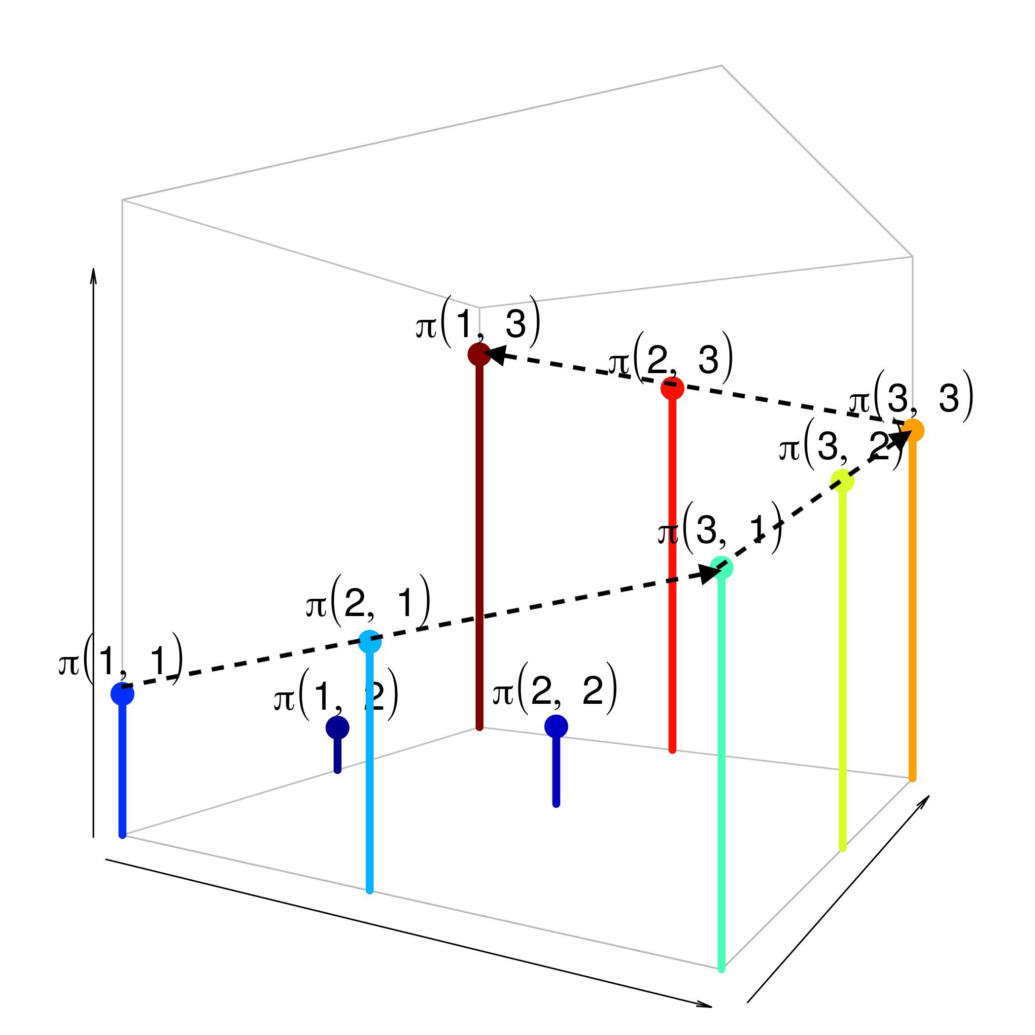
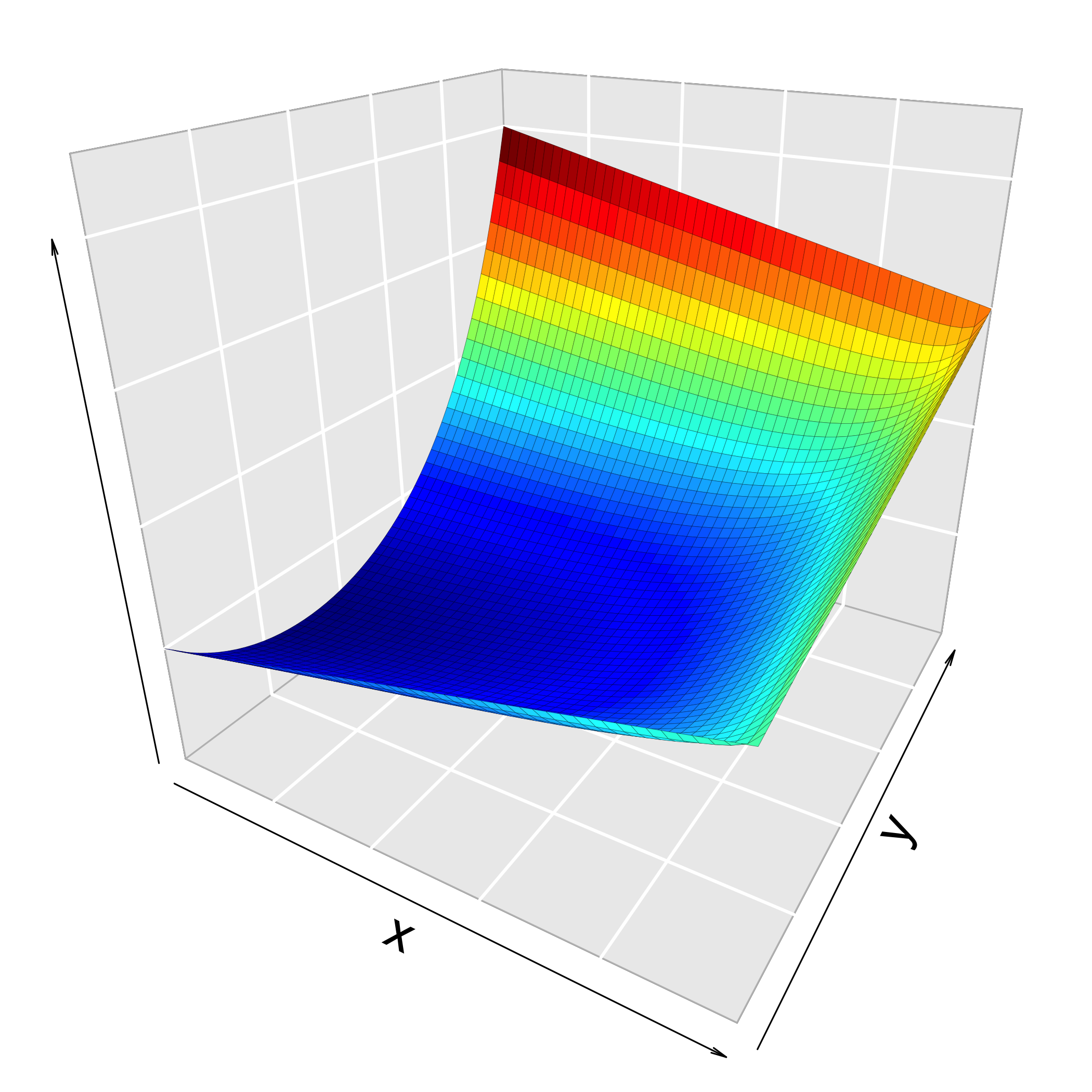
Figure 1: Left: a unimodal distribution defined on $\mathcal{X}=\{1,2,3\}^{2}$ (the height of each bar is the value of $\log\pi$). Right: a continuous analogue of the distribution shown in the left panel.

Appendix D Simulation Settings and Results

D.1 Weighted Permutations

Let $\mathcal{X}$ be the collection of all possible permutations of $\{1,\dots,p\}$. For each permutation $\tau\in\mathcal{X}$, let $\tau(i)$ be the index of the variable that has the $i$-th position in $\tau$ and $\tau^{-1}(k)$ be the ranking of the $k$-th variable. Assume that

$$\pi(\tau)\propto\prod_{k=1}^{p}W(k,\tau^{-1}(k)),$$

where $W\colon\mathcal{X}^{2}\rightarrow\mathbb{R}_{+}$ is a positive matrix, and

$$\log W(k,j)=-\eta\phi_{k}|j-\mu_{k}|\log p,\quad\forall\,j,k\in\{1,\dots,p\},$$

for some $\eta>0$, $\phi_{k}>0$ and $\mu_{k}\in[1,p]$. We interpret $\eta$ as the signal-to-noise ratio (SNR) parameter. Let $\mathcal{N}(\tau)$ be the set of all permutations that can be obtained from $\tau$ by a transposition; thus, $|\mathcal{N}(\tau)|=p(p-1)/2$. We simulate $W$ in two ways such that $\pi$ has one unique mode at $\tau^{*}=(1,\dots,p)$. In Scenario I, we draw $\mu_{k}\sim\mathrm{Unif}(k-0.1,k+0.1)$ and $\phi_{k}\sim\mathrm{Unif}(0.5,1)$ for $k=1,\dots,p$, independently. In Scenario II, we draw $\mu_{k}\sim\mathrm{Unif}(k-0.5,k+0.5)$ and $\phi_{k}\sim\mathrm{Unif}(0.1,1)$ for $k=1,\dots,p$, independently. We explain in the next paragraph why $\pi$ is unimodal in both scenarios. Loosely speaking, in Scenario I, $\pi$ decays at roughly the same rate in every direction, while in Scenario II, $\pi$ tends to be more irregular and decay very slowly in some directions, and some states in $\mathcal{N}(\tau^{*})$ can have posterior probabilities comparable to $\pi(\tau^{*})$. Thus, Scenario II represents a “weakly unimodal” setting where Assumption 1 is very likely to fail to hold for large $p$. We fix $p=100$, and for each scenario, we generate two instances of $\pi$, one with $\eta=1$ and the other with $\eta=2$.

In both scenarios, observe that for each $k$, $j\mapsto W(k,j)$ is unimodal with mode at $j=k$. To see that $\pi$ is guaranteed to be unimodal with mode at $\tau^{*}$, consider any permutation $\tau\neq\tau^{*}$. Let

$$j_{1}=\min\{1\leq i\leq p\colon\tau^{-1}(i)\neq i\},\text{ and }j_{\ell}=\tau^{-1}(j_{\ell-1})\text{ for }\ell=2,3,\dots.$$

Observe that $j_{2}>j_{1}$. If $j_{3}<j_{2}$, then we can swap the ranks of variables $j_{1}$ and $j_{2}$ and the new permutation will have a larger posterior probability. If $j_{3}>j_{2}$, let $m=\min\{\ell\geq 1\colon j_{\ell+1}<j_{\ell}\}$. Observe that $m<p$ and $j_{m+1}\geq j_{1}$. Hence, there exists some $1\leq s\leq m-1$ such that $j_{s}\leq j_{m+1}<j_{s+1}$. That is, $j_{s}\leq\tau^{-1}(j_{m})<\tau^{-1}(j_{s})<j_{m}$, which shows that we can increase the posterior probability by swapping variables $s$ and $m$.

We compare RWMH and Algorithm 1 with the following five choices of $h$: $h_{+1},h_{\wedge 1},h_{0.5}$, $h_{0.3}(u)=u^{0.3}$ and $h_{0.4}(u)=u^{0.4}$. For $k=1,\dots,p$, let $f_{k}(\tau)=\tau^{-1}(k)$ and consider the estimator $\hat{f}_{k}(t,\omega)$ defined in (4) (for RWMH, $\omega\equiv 1$, and for IIT samplers, $\omega=\pi/\pi_{h}$). The number of iterations $t$ is chosen to be $7\times 10^{5}$ for RWMH and $10^{3}$ for each IIT sampler so that the wall time used by each algorithm is about the same (the number of posterior evaluations does not dominate the empirical complexity in this study). For each instance of $\pi$, we run each sampler $100$ times and then calculate the variance of $\hat{f}_{k}$ for each $k$. Boxplots for $\{\mathrm{Var}(\hat{f}_{k})\}_{k=1}^{p}$ are shown in Figure 2. The simulation code is written in R.

From Figure 2, one can see that in Scenario I, the advantage of IIT schemes is overwhelming. In Scenario II with SNR $=1$, only the IIT scheme $h_{0.5}$ is arguably slightly better than RWMH, and the IIT schemes $h_{+1},h_{\wedge 1}$ and $h_{0.3}$ are clearly less efficient than RWMH. But when SNR increases to $2$, IIT schemes $h_{0.3},h_{0.4},h_{0.5}$ all perform significantly better than RWMH.

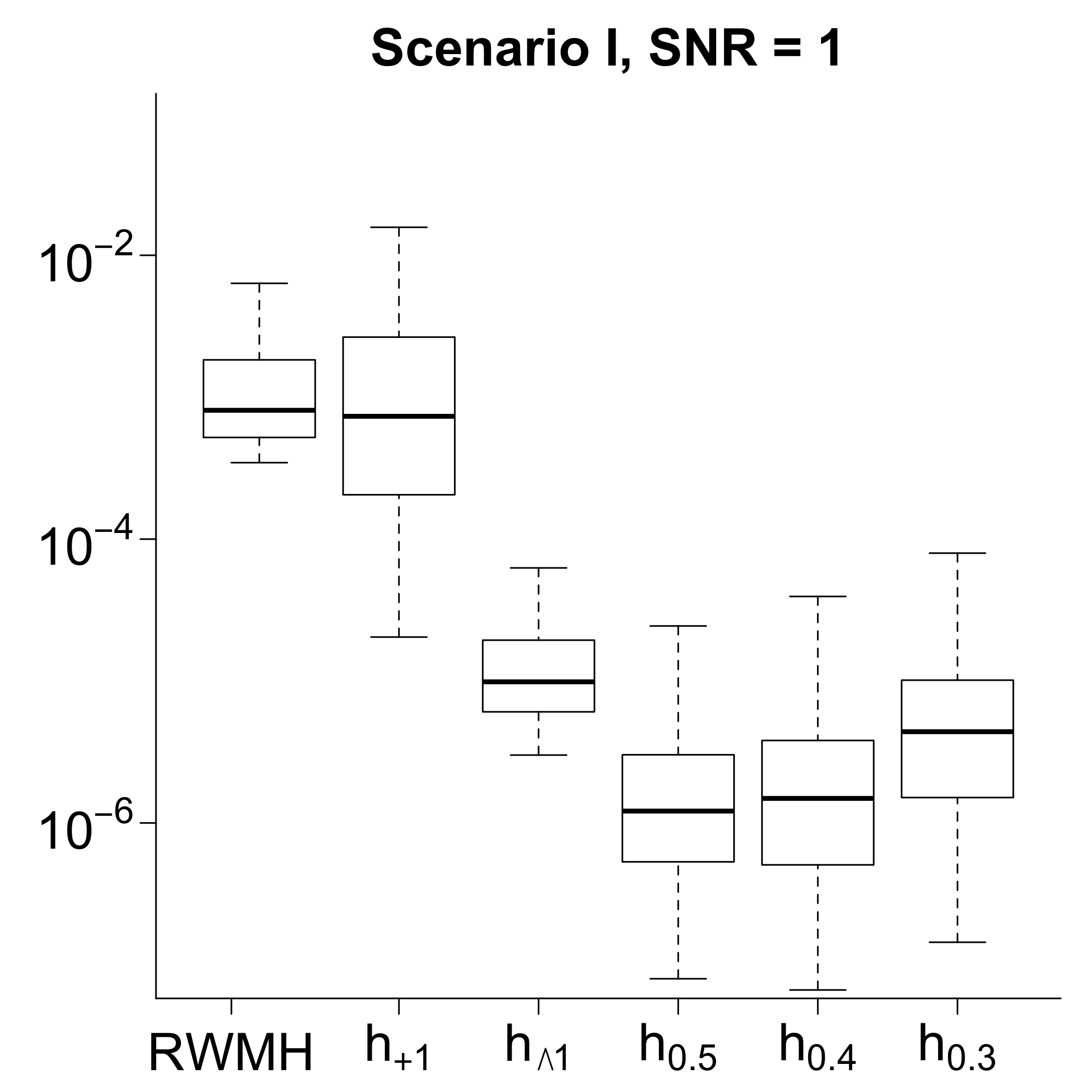
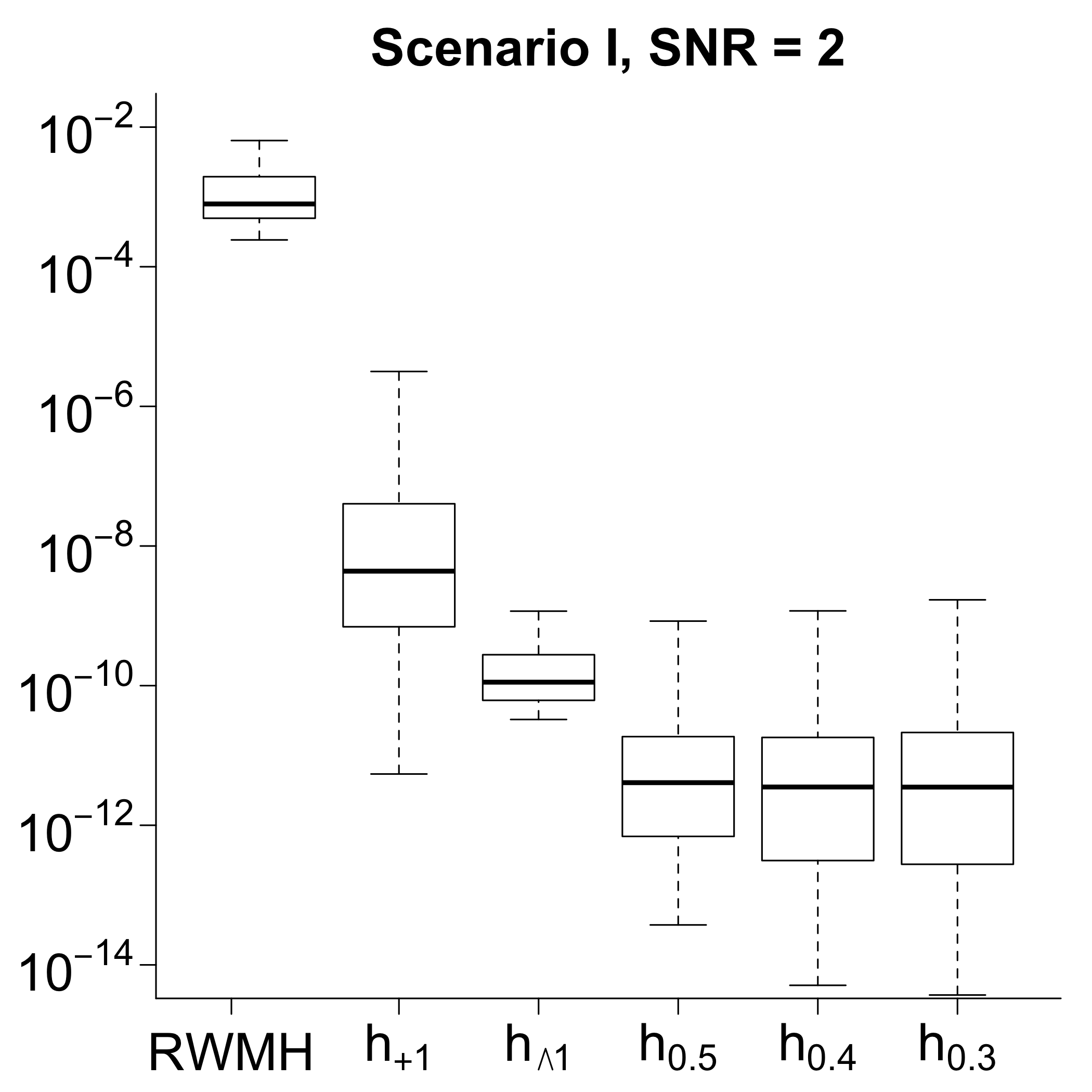
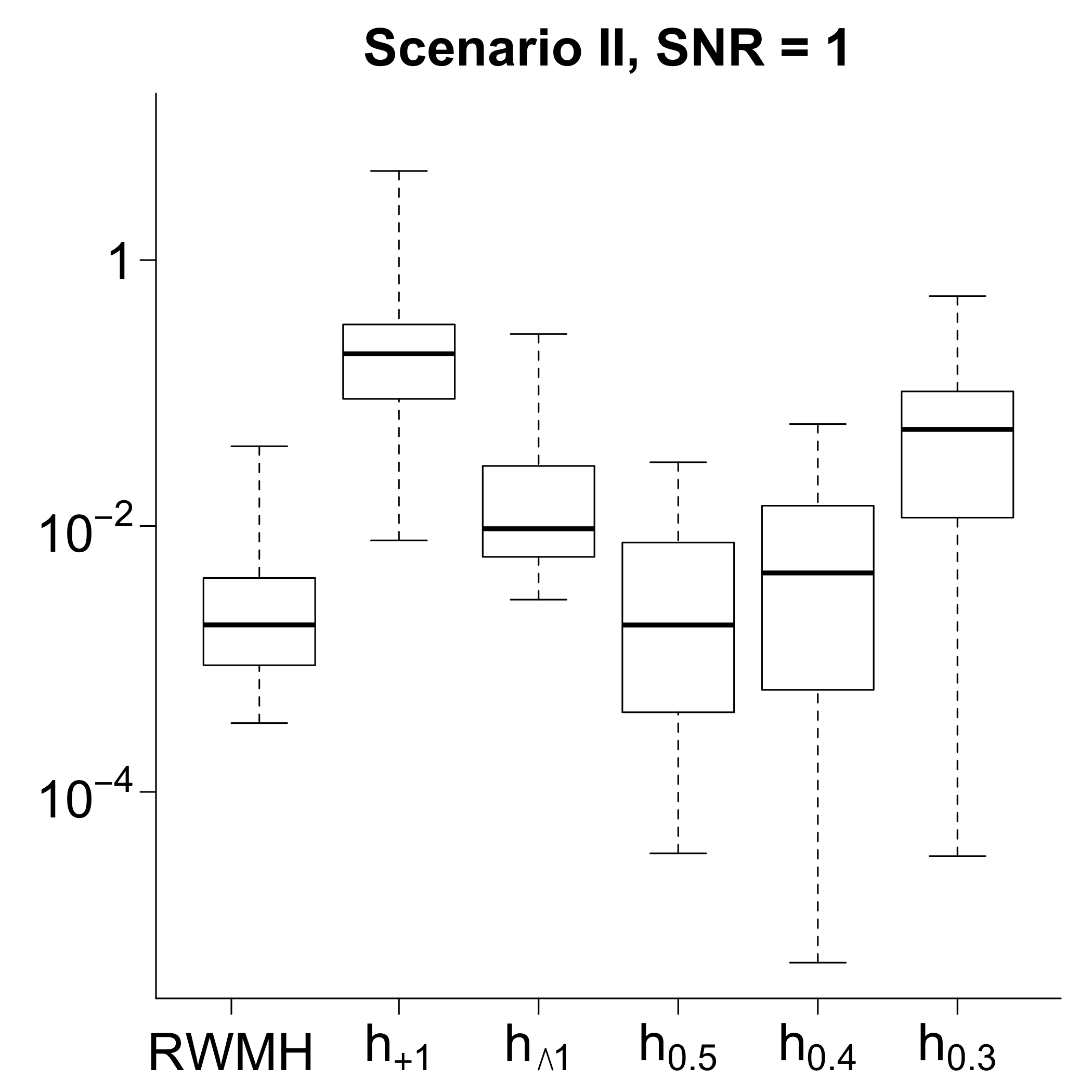
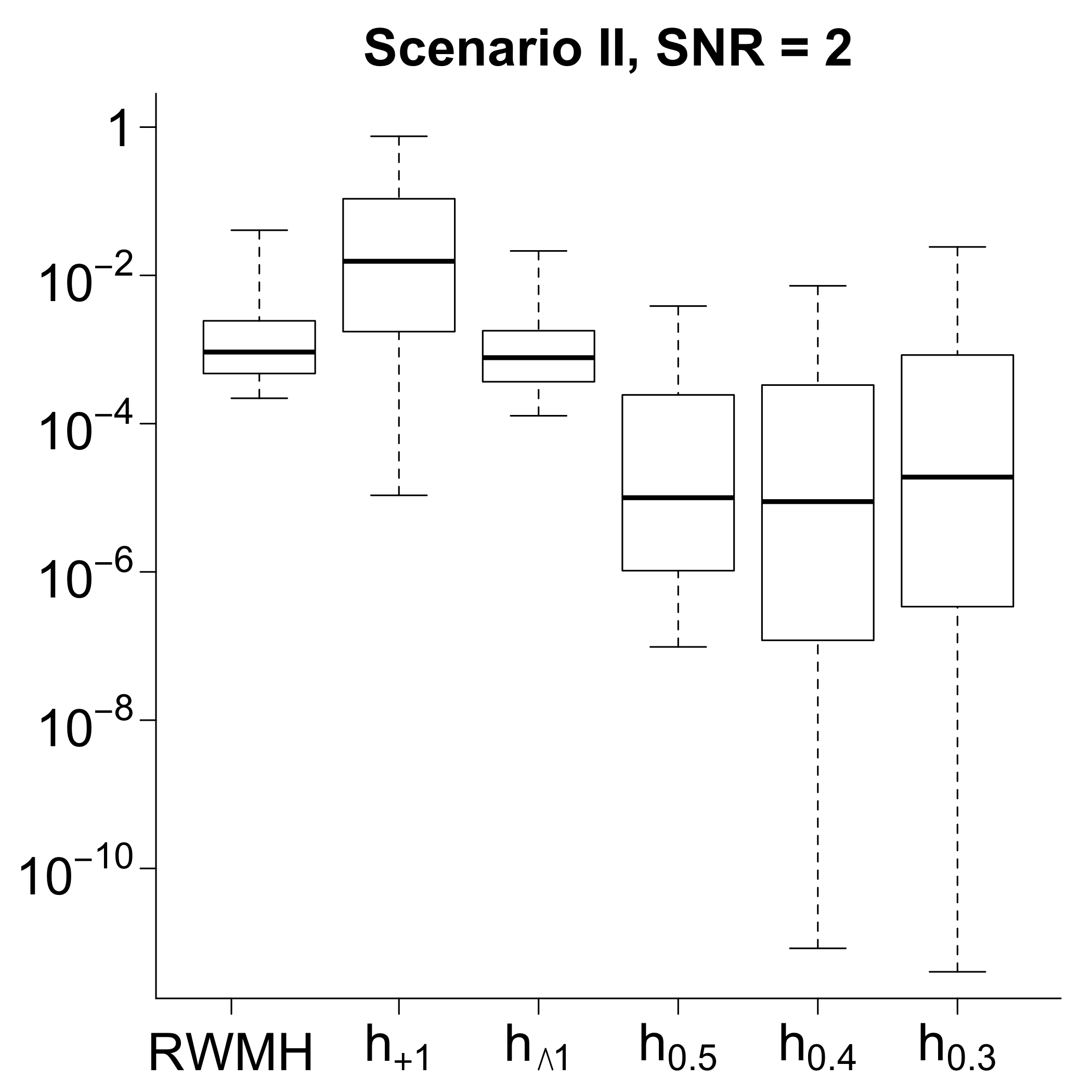
Figure 2: Each plot corresponds to one instance of $\pi$ for the “weighted permutations” problem with $p=100$. Each box gives the empirical distribution of $\{\mathrm{Var}(\hat{f}_{k})\}_{k=1}^{p}$ for one sampler, where $\mathrm{Var}(\hat{f}_{k})$ is calculated from 100 independent runs of the algorithm. Each RWMH run has $7\times 10^{5}$ iterations, which takes about $10.3$ seconds; each IIT run has $10^{3}$ iterations, which takes about $10.1$ seconds.

D.2 Variable Selection

We first describe how we simulate the data. Let $L\in\mathbb{R}^{n\times p}$ denote the design matrix. To mimic complex real-world problems with correlated predictors, we sample each row of $L$ independently from $N(0,\Sigma)$ where $\Sigma_{ij}=e^{-|i-j|}$ for each $(i,j)$. Generate the response $Y\in\mathbb{R}^{n}$ by

$$Y_{i}\overset{\mathrm{i.i.d.}}{\sim}N(\sum\nolimits_{j=1}^{j=s^{*}}\beta_{j}L_{ij},1),$$

where $s^{*}=20$ is the number of “causal” predictors. Generate $\beta$ by

$$\beta_{i}\overset{\mathrm{i.i.d.}}{\sim}\mathrm{SNR}\sqrt{\frac{\log p}{n}}\mathrm{Unif}((2,3)\cup(-3,-2)).$$

We use $\mathrm{SNR}=1,2,3$, and for each value of SNR, we simulate $100$ replicates of $(L,Y)$. This simulation setting is very similar to that used in Yang et al. (2016) (the main difference is that they used $s^{*}=10$).

As in Example 1, denote the state space by $\mathcal{X}=\{0,1\}^{p}$ (a hard threshold on the model size is unnecessary in our simulation since an MCMC sampler never visits extremely large models in all of our runs). We follow (Yang et al., 2016) to calculate the posterior distribution by

$$\pi(x)\propto p^{-c_{0}\lVert x\rVert_{1}}\frac{(1+g)^{-\lVert x\rVert_{1}/2}}{(1+g(1-R_{x}^{2}))^{n/2}},$$ (7)

where $R^{2}_{x}$ is the usual R-squared statistic for the model $x$, and $c_{0}$ is the hyperparameter in the sparsity prior on $x$, and $g$ is the hyperparameter in the g-prior. We fix $1+g=p^{3}$ and $c_{0}=2$ in our simulation.

We consider four IIT samplers with weighting scheme $h_{+1},h_{\wedge 1},h_{0.5}$ and $h_{0.3}$. For all of them, we use the neighborhood relation $\mathcal{N}^{1}$, which we recall only includes “addition” and “deletion” moves. Note $|\mathcal{N}^{1}(x)|=p$ for all $x$. For comparison, we consider the standard add-delete-swap MH sampler (denoted by ADS) with proposal distribution

$$K_{\rm{ads}}(x,y)=0.4\frac{\bm{1}_{\mathcal{N}_{\rm{add}}(x)}(y)}{|\mathcal{N}_{\rm{add}}(x)|}+0.4\frac{\bm{1}_{\mathcal{N}_{\rm{del}}(x)}(y)}{|\mathcal{N}_{\rm{del}}(x)|}+0.2\frac{\bm{1}_{\mathcal{N}_{\rm{swap}}(x)}(y)}{|\mathcal{N}_{\rm{swap}}(x)|}.$$

This is slightly different from a RWMH that proposes uniformly from $\mathcal{N}^{2}(x)$, since we fix the proposal probabilities of three types of moves to $0.4,0.4,0.2$. In the main text, we simply refer to this ADS sampler as RWMH.

For each simulated data set, we initialize all samplers at the same model consisting of 10 random covariates, and run ADS for $5\times 10^{6}$ iterations and each IIT sampler for $5\times 10^{3}$ iterations. Each IIT run takes less than $20$ seconds while ADS takes about $2,000$ seconds (it is likely that the code for ADS sampler can be further optimized, but due to overhead cost, our setting should already be very fair to ADS). The code for IIT sampling is written in C++.

Before we discuss the performance of five samplers, we investigate the shape of $\pi$ to verify whether the assumptions used in our theory approximately hold for this variable selection problem. Calculating $\pi$ at each $x\in\mathcal{X}$ is impossible since $|\mathcal{X}|=2^{p}\approx 10^{1505}$. So we empirically check the multimodality of $\pi$ by combining sample paths of all IIT runs. First, we count the number of local modes of $\pi$. We say a point $x$ is a local mode if $\pi(x)>\operatorname*{arg\,max}_{y\in\mathcal{N}^{1}(x)}\pi(y)$. When SNR $=2$ (intermediate SNR), among the 100 replicates, the number of local modes of $\pi$ (that have been visited by any sampler) ranges from $1$ to $12$ with an average of $5.3$. When SNR $=1$ or SNR $=3$, the number of local modes tends to be much smaller; see Figure 3. Next, we consider the quantity

$$\nu(x)=\max_{y\in\mathcal{N}^{1}(x)}\log_{p}\left(\frac{\pi(y)}{\pi(x)}\right).$$ (8)

Assumption 1 would hold if $\nu(x)>1$ for each $x\neq x^{*}$, and Theorem 2 suggests that we need at least $\nu(x)>2$ at most $x$ so that IIT schemes can achieve optimal convergence rates. We find that $\nu(x)$ is indeed large and greater than $2$ at most points in all the three SNR cases. See Figure 4 and Table 1.

For the variable selection problem, the accuracy of posterior estimation largely depends on whether the sampler is able to find the “best” model in its search. So, we compare the performance of samplers using $T_{\hat{x}}$, where $\hat{x}$ denotes the model with the largest posterior probability that has been visited by any sampler (ADS or IIT) and $T_{\hat{x}}$ denotes the number of iterations taken by a sampler to find $\hat{x}$. See Figure 5 for the distribution of $T_{\hat{x}}$ for each sampler.

When SNR $=3$, $\pi$ tends to be unimodal with true model $x^{*}$ being the unique mode. In this case, IIT schemes $h_{\wedge 1},h_{0.5}$ and $h_{0.3}$ find $x^{*}$ very quickly and within $\approx 30$ iterations in most cases. This is expected since we initialize the sampler at some random $x$ with $\lVert x\rVert_{1}=10$ (so it takes about $10$ iterations to remove the non-influential covariates and $20$ iterations to add the influential ones). When SNR $=1$, $\pi$ is still likely to be unimodal, but the mode may be the empty model (or some other model with very small size) due to the weak signal size. This is why ADS sometimes can be very efficient since it only needs to remove the 10 non-influential covariates in the initial model. However, we still observe that $h_{0.5}$ and $h_{0.3}$ have better performance. The intermediate SNR case is the most challenging since $\pi$ is usually multimodal. We observe that the advantage of IIT schemes $h_{0.5}$ and $h_{0.3}$ is very significant in the sense that ADS often fails to find $\hat{x}$ in $5\times 10^{6}$ iterations; see Table 2. The best sampler in this case appears to be $h_{0.3}$ since it is most robust.

The IIT scheme $h_{+1}$ performs worse than ADS in all the three cases. Zanella and Roberts (2019) also noted that the naive TGS sampler (i.e., IIT scheme $h_{+1}$) may converge slowly for variable selection, and thus they proposed to use a weighted TGS algorithm, which yielded excellent performance. In addition, they used Rao-Blackwellization to reduce the variance of posterior estimation. We note that both schemes are highly effective but rely on the specific structure of $\mathcal{X}$ in variable selection. The same Rao-Blackwellization scheme can also be applied to IIT, but we did not observe significant improvement.

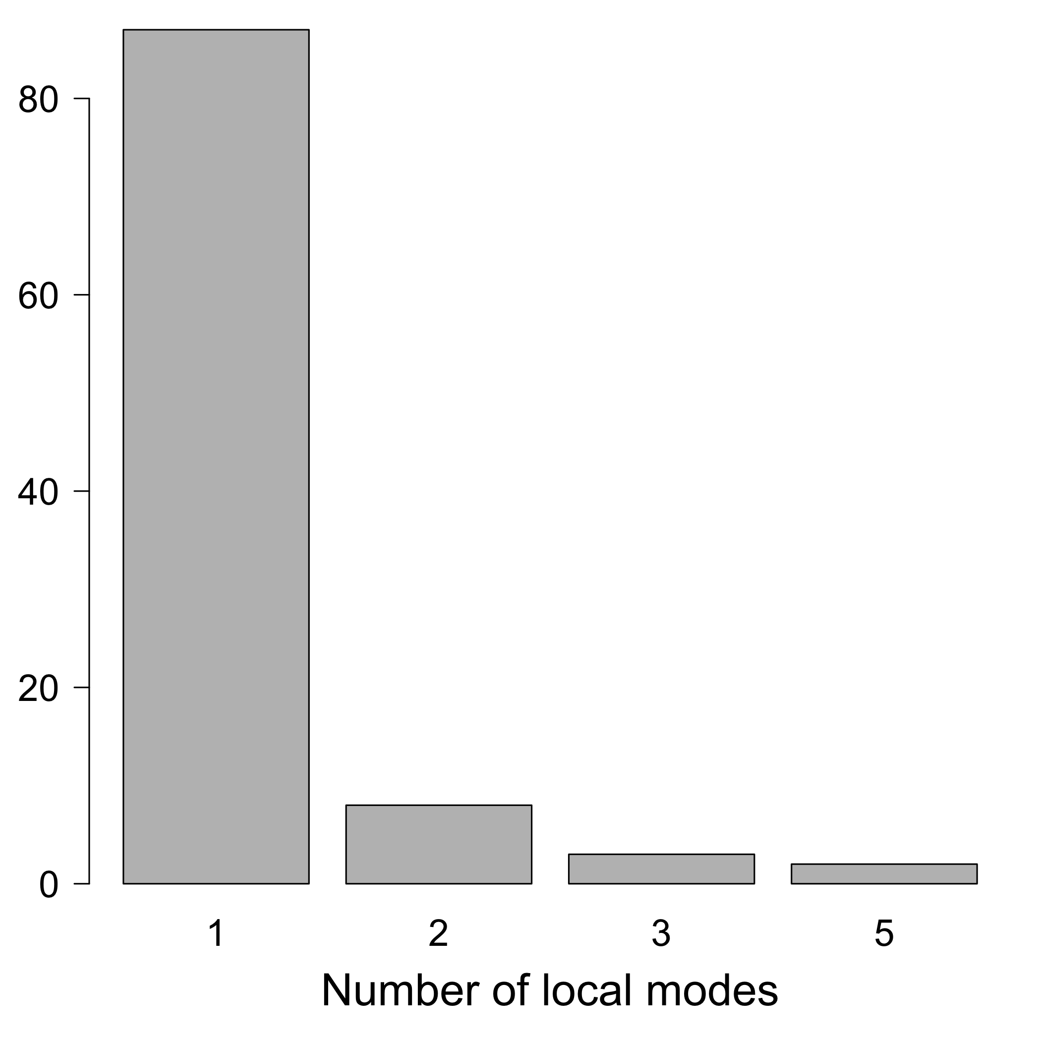
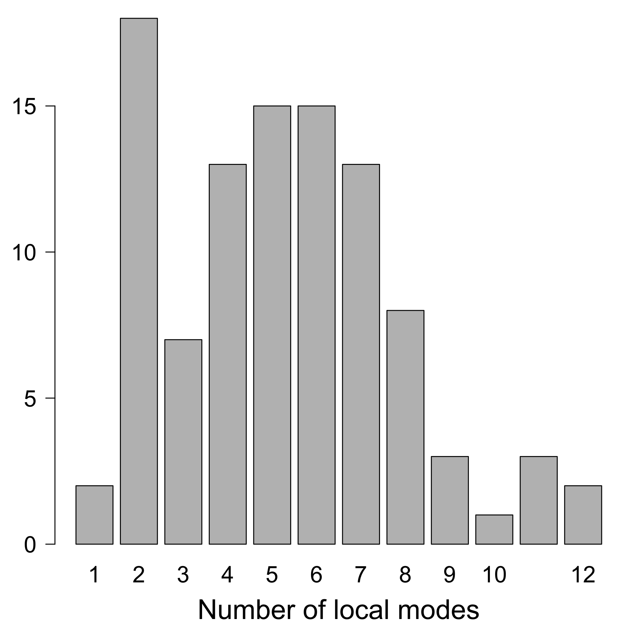
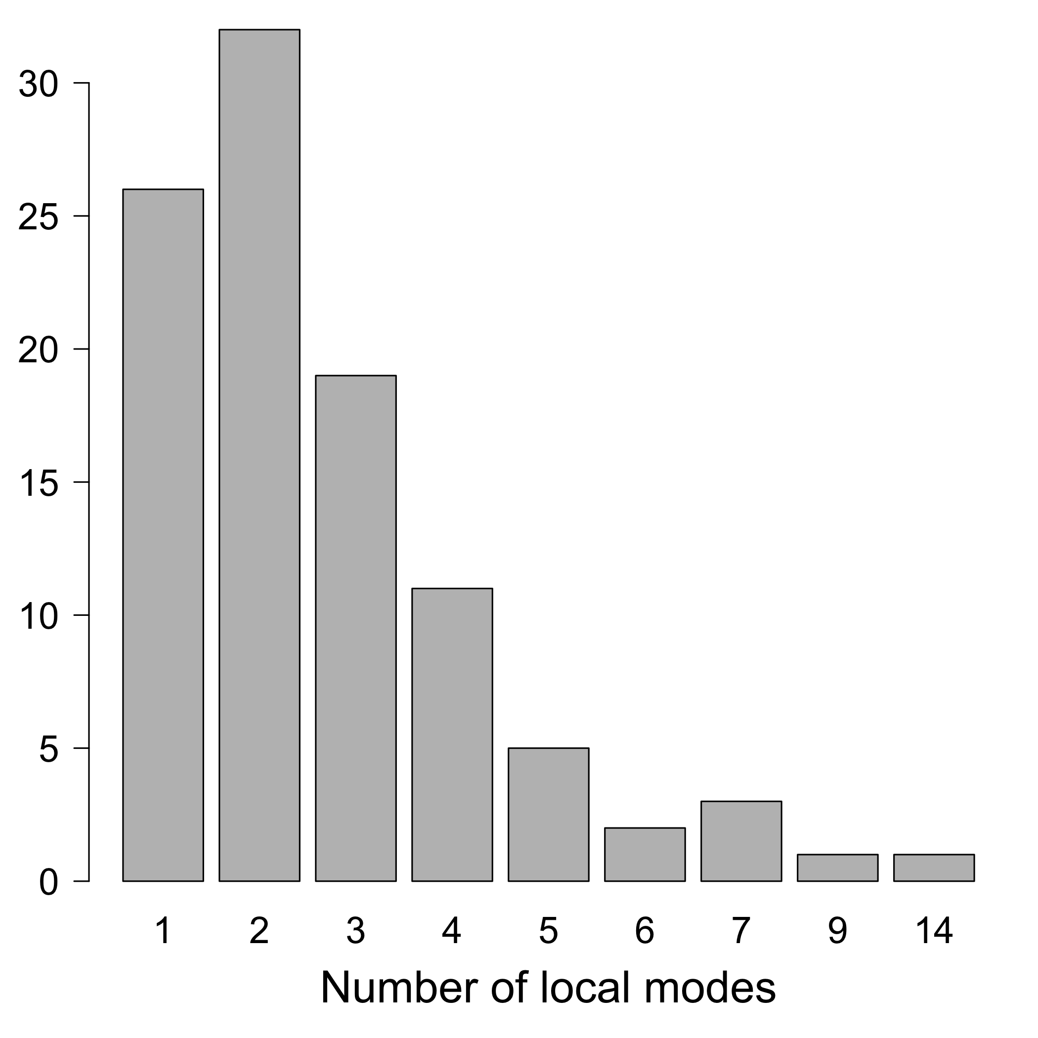
Figure 3: Distribution of the number of local modes in the variable selection simulation study. Left: SNR $=3$; middle: SNR $=2$; right: SNR $=1$. For each value of SNR, we count the number of local modes of $\pi$ (visited by any IIT sampler) for 100 simulated data sets.

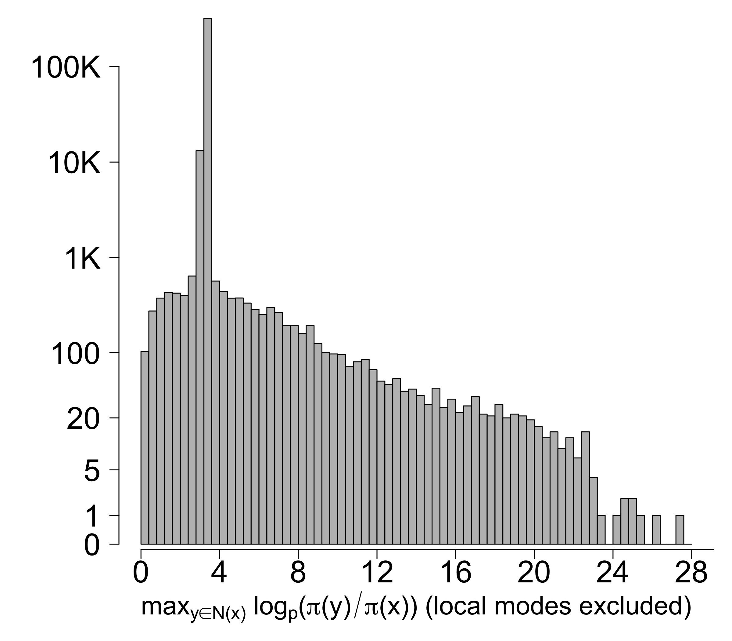
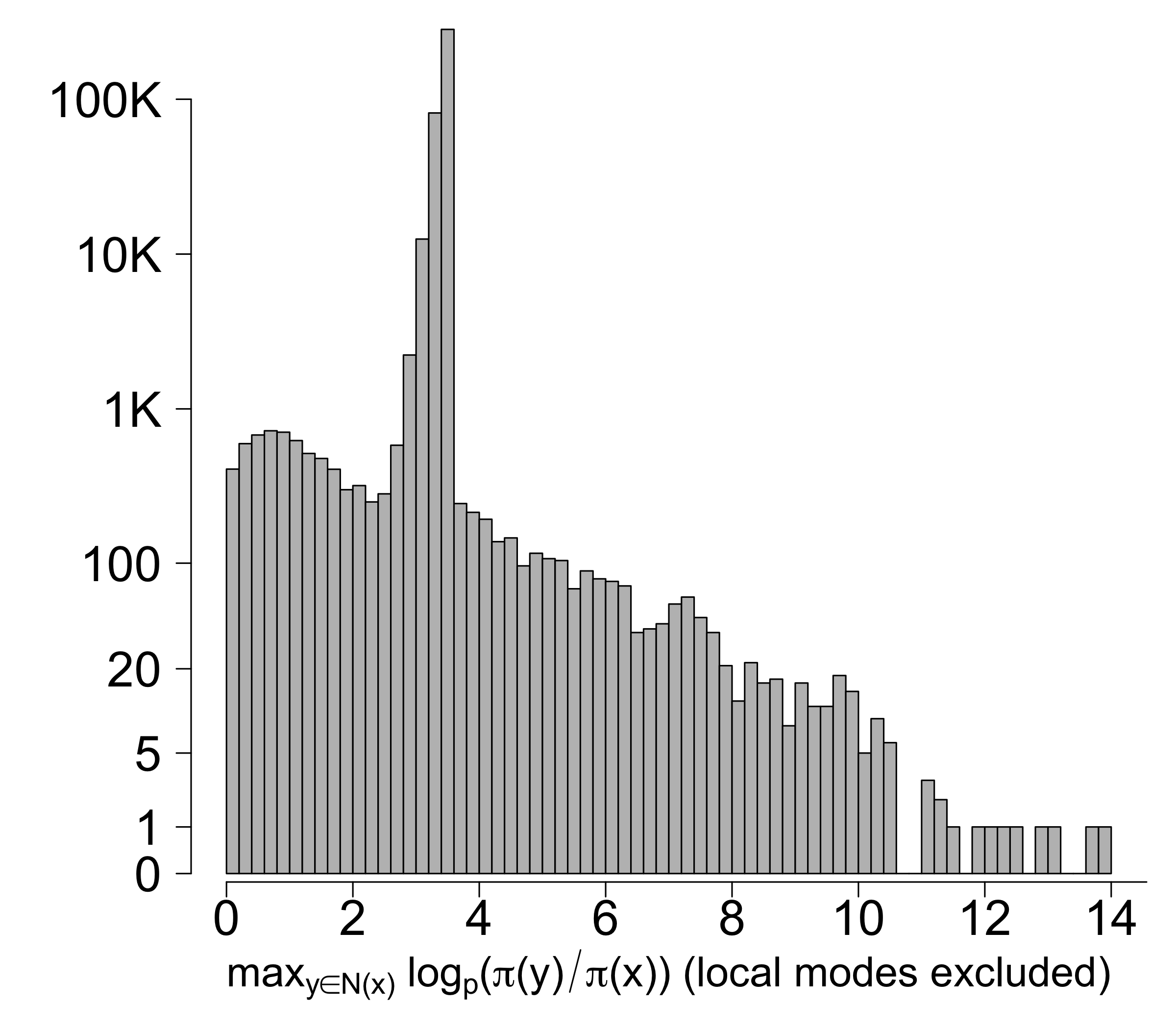
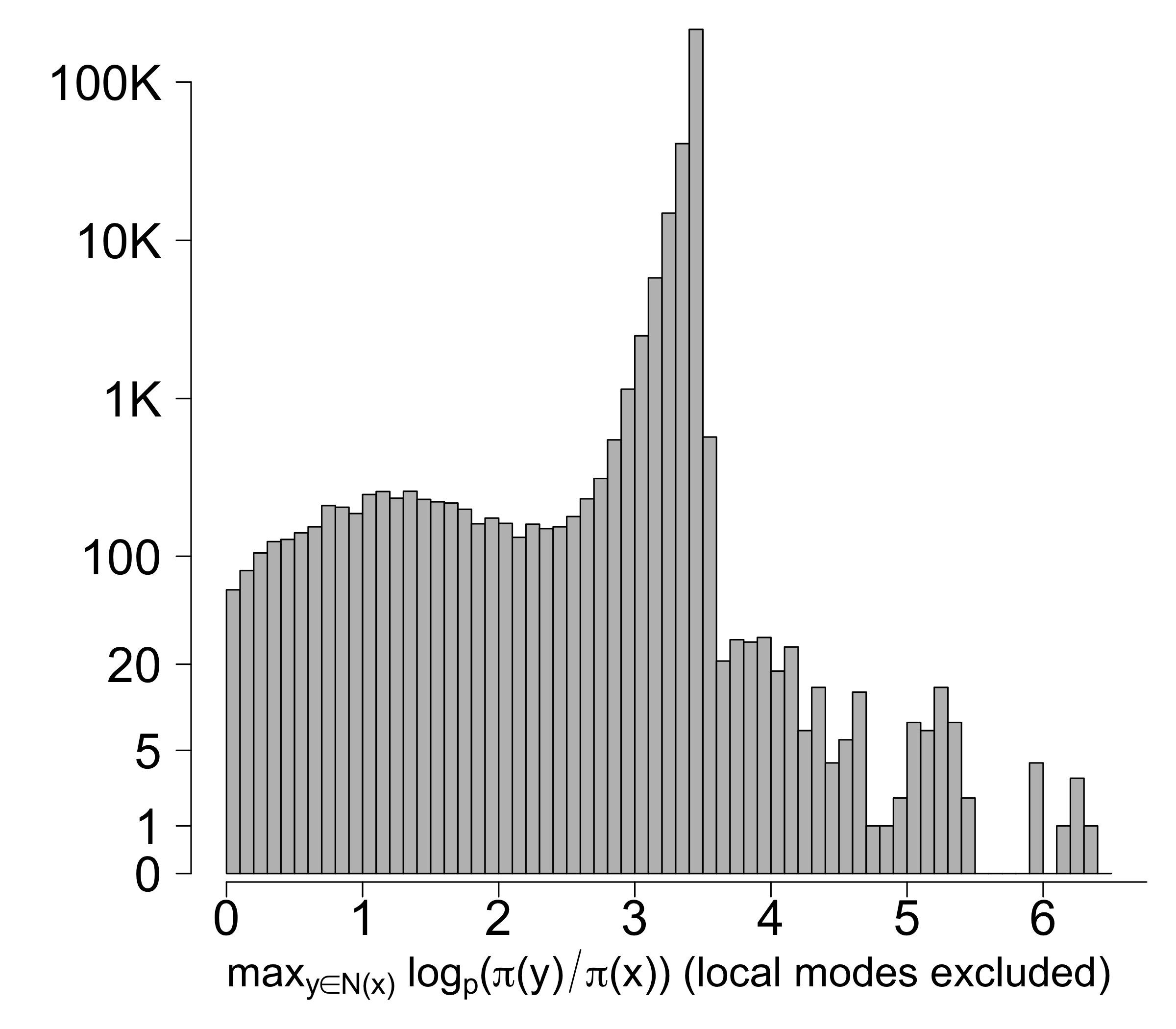
Figure 4: Distribution of $\nu(x)$ in the variable selection simulation study. Left: SNR $=3$; middle: SNR $=2$; right: SNR $=1$. For each value of SNR, we pool together the sample paths of IIT samplers for all 100 simulated data sets.

SNR	$\nu(x)>1$	$\nu(x)>2$	$\nu(x)>3$
SNR $=3$	99.8%	99.5%	98.7%
SNR $=2$	99.1%	98.5%	97.5%
SNR $=1$	99.4%	98.7%	97.5%

Table 1: Distribution of $\nu(x)$. For each SNR, we report the percentage of points $x$ with $\nu(x)>c$ for $c=1,2,3$ using the data shown in Figure 4 (local modes are included in this calculation).

SNR	ADS	$h_{+1}$	$h_{\wedge 1}$	$h_{0.5}$	$h_{0.3}$
SNR $=3$	0	2	0	0	0
SNR $=2$	38	72	15	10	1
SNR $=1$	1	10	1	0	0

Table 2: Number of experiments (out of 100) where the sampler fails to find $\hat{x}$ in the entire run. This supplements Figure 5.

SNR $=3$


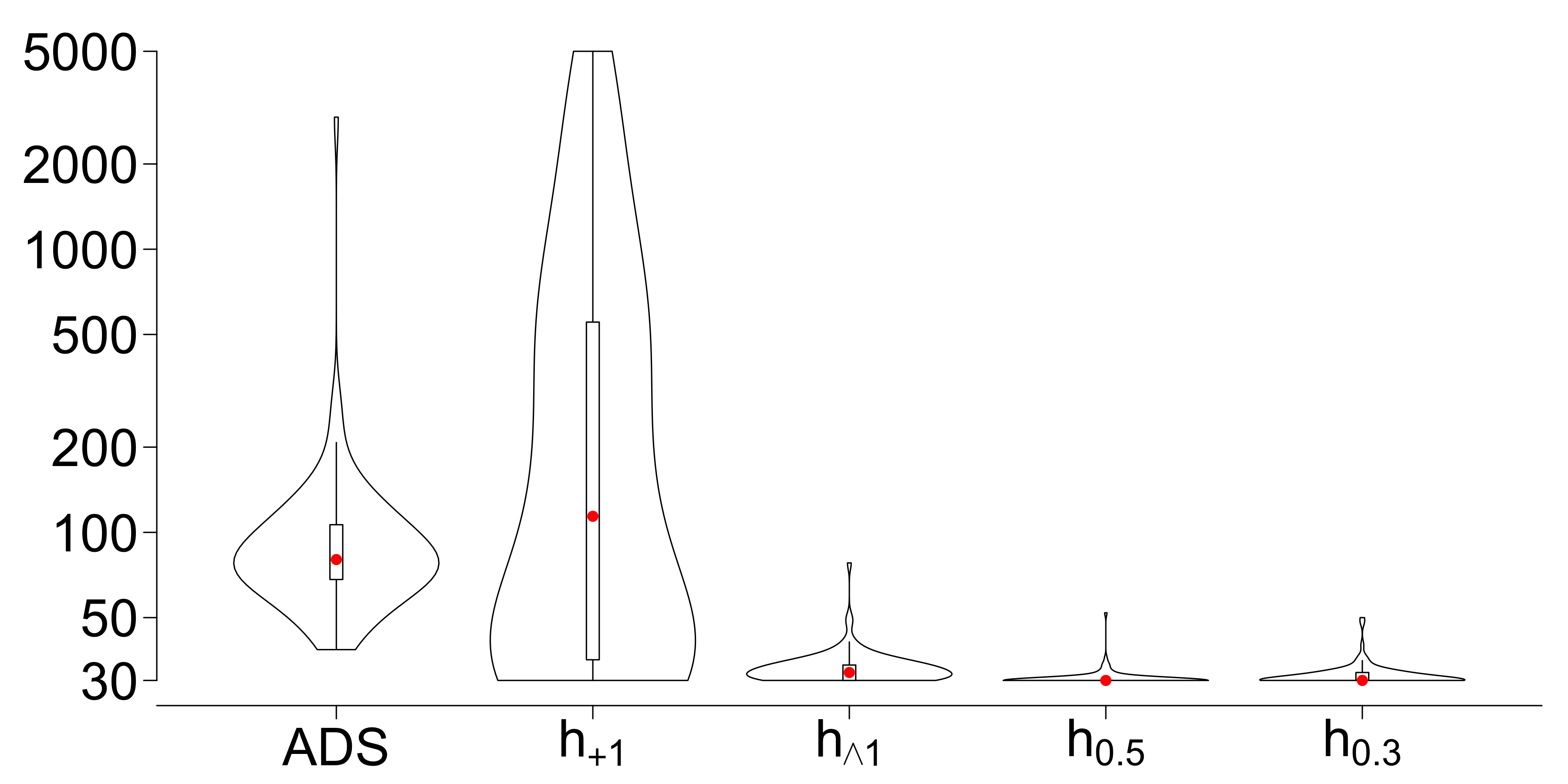
SNR $=2$


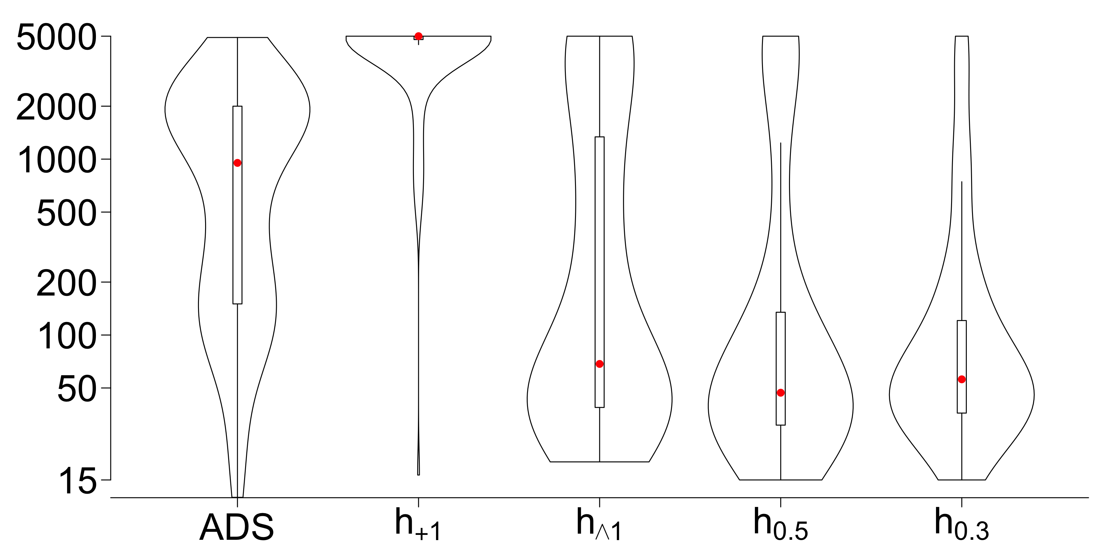
SNR $=1$

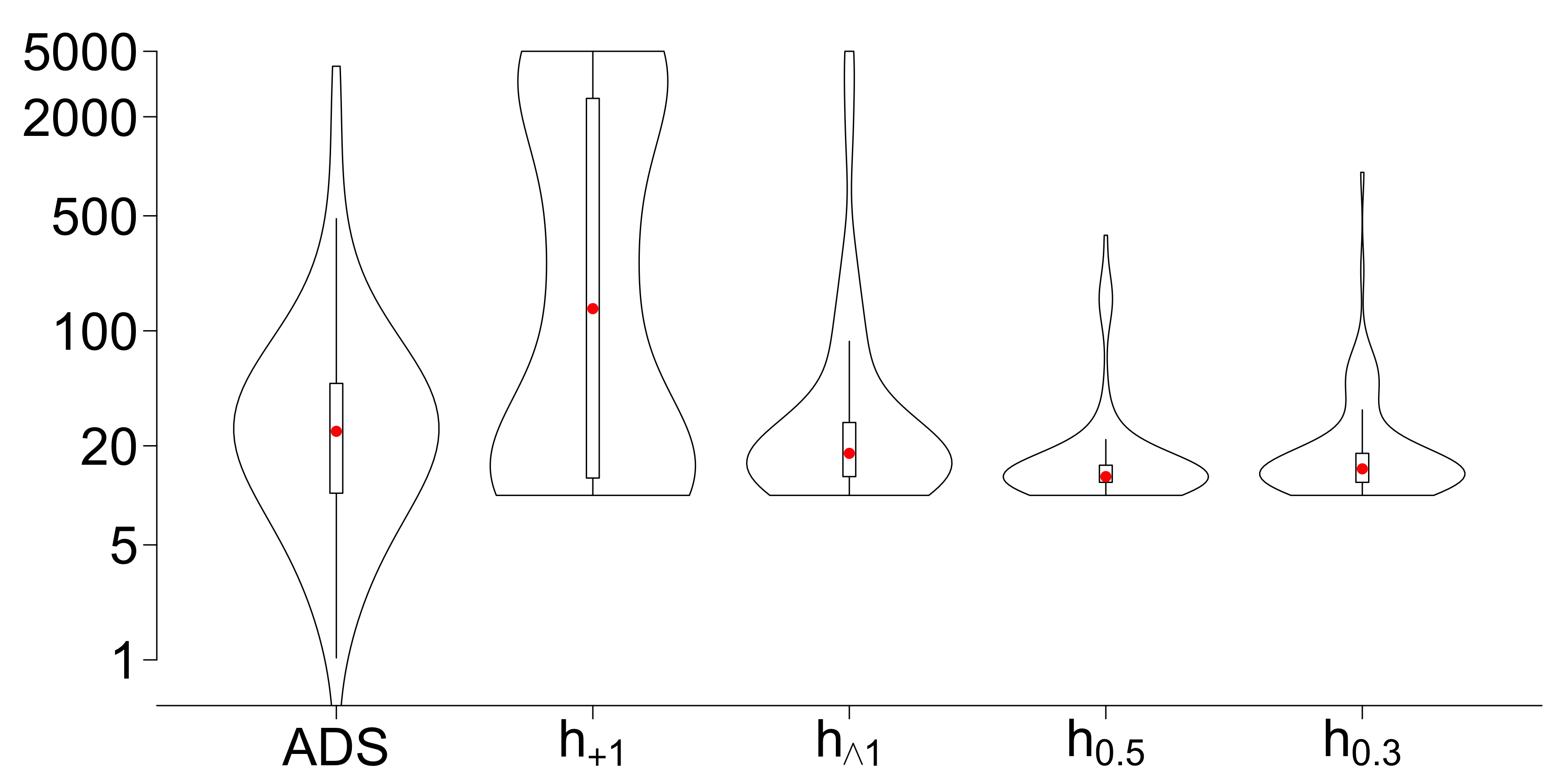
Figure 5: Violin plots for the distribution of $T_{\hat{x}}$ in 100 replicates. The numbers on the y-axis correspond to $T_{\hat{x}}$ for IIT samplers and $T_{\hat{x}}\times 10^{-3}$ for ADS. $T_{\hat{x}}$ is truncated at $5\times 10^{3}$ for IIT and $5\times 10^{6}$ for ADS. The plot is made using R package vioplot. A boxplot is drawn inside each violin: the red dot denotes the median and the rectangle corresponds to the interquartile range. Note that the width of each violin is forced to be the same.

Appendix E Examples in the Main Text

E.1 Details of Example 3

We show how to derive the expression for $\omega$. First, observe that

$$1=\sum_{k=1}^{p}\pi(k)\leq\pi(0)+\pi(1)+\pi(1)r^{-1}+\cdots+\pi(1)r^{-(p-1)}\leq\pi(0)+\frac{\pi(1)}{1-r^{-1}}.$$

Since $\pi(0)=\pi(1)$ and $r\rightarrow\infty$, we get $\pi(0)=\pi(1)\sim 1/2$, and for $k\geq 2$, $\pi(k)\lesssim r^{-(k-1)}/2$. For $h(u)=u^{a}$ with some fixed $a>0$, we have

$$\sum_{x\in\mathcal{X}}\pi(x)^{2a}Z_{h}(x)=\sum_{x\in\mathcal{X}}\sum_{y\in\mathcal{N}(x)}\pi(x)^{a}\pi(y)^{a}=\sum_{k=0}^{p-1}2\pi(k)^{a}\pi(k+1)^{a}.$$

Observe that as $k$ grows, $\pi(k)^{a}\pi(k+1)^{a}$ decreases at a rate not slower than $r^{-a}$. Therefore, as $r\rightarrow\infty$, we obtain that

$$\sum_{x\in\mathcal{X}}\pi(x)^{2a}Z_{h}(x)\sim 2\pi(0)^{a}\pi(1)^{a}\sim 2^{1-2a}.$$

By Lemma 1,

$$\pi_{h}(k)=\frac{\pi(k)^{2a}Z_{h}(k)}{\sum_{x\in\mathcal{X}}\pi(x)^{2a}Z_{h}(x)}\sim\left\{\begin{array}[]{cc}\frac{\pi(k-1)^{a}\pi(k)^{a}}{2^{1-2a}},&k=2,\dots,p,\\ 1/2,&k=0,1.\end{array}\right.$$

The importance weight $\omega$ then can be calculated by $\omega(k)=\pi(k)/\pi_{h}(k)$.

E.2 Details of Example 4

Define a function $f\colon\mathcal{X}\rightarrow\{-1,1\}$ by letting $f(x)=1$ if $x_{1}=1$ and $f(x)=-1$ if $x_{1}=0$. We show that $f$ is an eigenvector of $Q_{h}$ with eigenvalue $-2/p$, which proves $\mathrm{Gap}(Q_{h})\leq 2/p$. We use the notation $y^{(i)}(x)$ defined in (6). For any $x$ with $x_{1}=1$, $f(y^{(i)}(x))=1$ for any $i\geq 2$, and $f(y^{(1)}(x))=-1$. Hence,

$$\sum_{x\in\mathcal{X}}Q_{h}(x,y)f(y)=\sum_{i=2}^{p}Q_{h}(x,y^{(i)}(x))-Q_{h}(x,y^{(1)}(x))+Q_{h}(x,x)=-2Q_{h}(x,y^{(1)}(x)).$$

Using $\pi(y^{(1)}(x))=\pi(x)$ and (18), we find that $Q_{h}(x,y^{(1)}(x))=2/\mathbb{E}_{\pi}[Z_{h}]$. Since $|\mathcal{N}^{1}(x)|=p$ for every $x$, we get $\mathbb{E}_{\pi}[Z_{h}]=2p$ from (19), and thus $\sum_{x\in\mathcal{X}}Q_{h}(x,y)f(y)=-2/p$. The case $x_{1}=0$ follows by an analogous calculation.

Appendix F A Generic Mixing Time Bound for Decomposable Markov Chains

Lemma 4.

Consider the transition kernel $P$ of a $\frac{1}{2}$-lazy discrete-time Markov chain with unique stationary measure $\pi$ on state space $\mathcal{X}$. Denote by $\mathcal{X}=\sqcup_{i=1}^{M}\mathcal{X}_{i}$ a decomposition of the state space, and denote by $x_{i}^{*}\in\mathcal{X}_{i}$ a privileged point satisfying $\pi(x_{i}^{*})/\pi(\mathcal{X}_{i})>0.65$ for each $i\in\{1,2,\ldots,M\}$. Define $\mathcal{X}^{*}=\cup_{i=1}^{M}x_{i}^{*}$ to be the collection of all privileged points. Let $P|_{\mathcal{X}_{i}}$ denote the trace of $P$ on $\mathcal{X}_{i}$. Then there exists a universal constant $C$ so that

$$\tau_{\mathrm{mix}}(P)\leq C\,\max\left\{\mathrm{Gap}_{\rm{min}}^{-1}\,M\,\log\frac{8M}{\pi_{\mathrm{min}}},\,\tau_{\mathrm{mix}}(P|_{\mathcal{X}^{*}})\right\},$$

where $\mathrm{Gap}_{\rm{min}}=\min_{i\in\{1,2,\ldots,M\}}\mathrm{Gap}(P|_{\mathcal{X}_{i}})$ and $\pi_{\mathrm{min}}=\min_{x\in\mathcal{X}}\pi(x)$ .

Proof.

Let $\mathbb{P}_{x}$ denote the probability measure corresponding to a Markov chain $\{X_{t}\}_{t\geq 0}$ with transition matrix $P$ and $X_{0}=x$. Let $\{X^{(k)}_{t}\}_{t\geq 0}$ denote the trace of $\{X_{t}\}$ on $\mathcal{X}_{k}$, as defined in Definition 3. Let $\pi_{i}(\cdot)=\pi(\cdot)/\pi(\mathcal{X}_{i})$ denote the stationary distribution of $P|_{\mathcal{X}_{k}}$. By assumption, we have $\mathbb{E}_{\pi_{i}}[\bm{1}_{\{x_{i}^{*}\}}(X^{(i)}_{t})]=\pi_{i}(x_{i}^{*})\geq 0.65$. By the Chernoff-like bound Lezaud (1998, Theorem 1.1),

$$\mathbb{P}_{x}[|\{t\in\{1,2,\dots,T\}\colon X_{t}^{(i)}\neq x^{*}_{i}\}|\geq 0.5T]\leq\frac{2}{\pi(x)}\exp\left(-\frac{\mathrm{Gap}(P|_{\mathcal{X}_{i}})}{56}T\right\}.$$ (9)

For $i\in\{1,2,\ldots,M\}$ and $T\in\mathbb{N}$, denote by $\mathcal{O}_{T}(i)=|\{0\leq t\leq T\,:\,X_{t}\in\mathcal{X}_{i}\}|$ the number of steps that the chain spends in $\mathcal{X}_{i}$. Denote by

$$\mathcal{G}_{T}=\left\{i\in\{1,2,\ldots,M\}\,:\,\mathcal{O}_{T}(i)>56\,\mathrm{Gap}_{\rm{min}}^{-1}\,\log\left(\frac{8M}{\pi_{\mathrm{min}}}\right)\right\}$$

the collection of indices for which this occupation time is large relative to the relaxation time. By the union bound, for all $x\in\mathcal{X}$:

$$\mathbb{P}_{x}\left[\forall\,i\in\mathcal{G}_{T},\,|\{0\leq t\leq T\,:\,X_{t}^{(i)}=x_{i}^{*}\}|>\frac{1}{2}\mathcal{O}_{T}(i)\right]\geq 0.75.$$ (10)

By the pigeonhole principle, for $T\geq T_{1}=(5M)56\,\mathrm{Gap}_{\rm{min}}^{-1}\,\log\left(\frac{8M}{\pi_{\mathrm{min}}}\right)$, we must have

$$|\{0\leq t\leq T\,:\,X_{t}\in\cup_{i\in\mathcal{G}_{T}}\mathcal{X}_{i}\}|\geq\frac{4}{5}T.$$

Combining this with inequality (10), we conclude that for all $T\geq T_{1}$, we have

$$\mathbb{P}_{x}\left[|\{0\leq t\leq T\colon X_{t}\in\mathcal{X}^{*}\}|\geq\frac{2}{5}T\right]>0.75.$$ (11)

Next, for set $S\subset\mathcal{X}^{*}$, define

$$\tilde{\tau}_{\mathrm{hit}}(S)=\min\{t\,:\,\tilde{X}_{t}\in S\}.$$

Denote by $\tau_{\mathrm{hit}}$ the analogous hitting time for the original chain. Fix an arbitrary subset $S\subset\mathcal{X}$ with $\pi(S)>0.45$. Since $\pi(\mathcal{X}^{*})\geq 0.65$, we have $\pi(S\cap\mathcal{X}^{*})>0.1$. For any $x\in\mathcal{X}$, we have

$$\mathbb{P}_{x}[\tilde{\tau}_{\mathrm{hit}}(S)\leq 4\tau_{\mathrm{mix}}(P|_{\mathcal{X}^{*}})] \geq\mathbb{P}_{x}[\tilde{X}_{4\tau_{\mathrm{mix}}(P|_{\mathcal{X}^{*}})}\in S]$$

$$\geq\pi|_{\mathcal{X}^{*}}(S\cap\mathcal{X}^{*})-\|P|_{\mathcal{X}^{*}}^{4\tau_{\mathrm{mix}}(P|_{\mathcal{X}^{*}})}(x,\cdot)-\pi|_{\mathcal{X}^{*}}(\cdot)\|_{\mathrm{TV}}$$

$$\geq 0.1-2^{-4}$$

$$\geq 0.03.$$

Iterating, for any $S\subset\mathcal{X}$ with $\pi(S)>0.45$, we have for $k\in\mathbb{N}$,

$$\max_{x\in\mathcal{X}}\mathbb{P}_{x}[\tilde{\tau}_{\mathrm{hit}}(S)>4k\,\tau_{\mathrm{mix}}(P|_{\mathcal{X}^{*}})]\leq 0.97^{k}.$$ (12)

Consider an integer

$$T\geq\max\left\{\frac{T_{1}}{5},\,\frac{2\log(4)}{-\log(0.97)}\tau_{\mathrm{mix}}(P|_{\mathcal{X}^{*}})\right\}.$$

Using a union bound and then combining inequalities (11) and (12), we have:

$$\max_{x\in\mathcal{X}}\mathbb{P}_{x}[\tau_{\mathrm{hit}}(S)>5T] \leq\max_{x\in\mathcal{X}}\mathbb{P}_{x}[|\{1\leq t\leq 5T\,:\,X_{i}\notin\mathcal{X}^{*}\}|>3T]+\max_{x\in\mathcal{X}}\mathbb{P}_{x}[\tilde{\tau}_{\mathrm{hit}}(S)>2T]$$

$$\leq 0.25+0.25$$

$$\leq 0.5.$$

Thus, for each $k\in\mathbb{N}$,

$$\max_{x\in\mathcal{X}}\mathbb{P}_{x}[\tau_{\mathrm{hit}}(S)>5kT]\leq 2^{-k}.$$

It follows that

$$\max_{x\in\mathcal{X}}\max_{S\subset\mathcal{X}\,:\,\pi(S)>0.6}\mathbb{E}_{x}[\tau_{\mathrm{hit}}(S)]\leq 10T.$$

Applying the main result of Peres and Sousi (2015) completes the proof. ∎

Appendix G Proofs

G.1 Proof of Lemma 1

Proof.

It suffices to check the detailed balance condition. If $h(u)=u^{a}$, then for any $y\in\mathcal{N}(x)$,

$$\pi(x)^{2a}Z_{h}(x)K_{h}(x,y)=\pi(x)^{2a}h\left(\frac{\pi(y)}{\pi(x)}\right)=\pi(x)^{a}\pi(y)^{a}=\pi(y)^{2a}Z_{h}(y)K_{h}(y,x).$$

Hence, $\pi_{h}\propto Z_{h}\cdot\pi$. Similarly, if $h$ is a balancing function, one can use Definition 1 to show that $\pi(x)Z_{h}(x)K_{h}(x,y)=\pi(y)Z_{h}(y)K_{h}(y,x)$. ∎

G.2 Proof of Lemma 2

Proof.

Without loss of generality, we can assume that $x^{(0)}$ is generated from $\pi_{h}$, since the limiting distribution of the estimator (4) does not depend on the initial distribution (Douc et al., 2018, Chapter 22.5). Let $W^{(0)},W^{(1)},\dots,W^{(t)}$ denote random variables such that given $x^{(k)}$, $W^{(k)}$ is an exponential random variable with mean $\omega(x^{(k)})$ and independent of everything else. Define

$$\hat{f}_{Q}(T_{m})=\frac{\sum_{k=0}^{m}f(x^{(k)})W^{(k)}}{T_{m}},\quad\quad\text{ where }T_{m}=\sum_{k=0}^{m}W^{(k)}.$$

Now one can see that Proposition 5 of Deligiannidis and Lee (2018) differs from our setting only in that the former assumes each $W^{(k)}$ is geometrically distributed (c.f. Doucet et al., 2015, Proposition 2). So, we can apply their argument. Since $\omega=\pi/\pi_{h}$, by the law of large numbers and central limit theorem for ergodic Markov chains (Häggström and Rosenthal, 2007, Corollary 6),

$$\frac{1}{t}\sum_{k=1}^{t}\omega(x^{(k)})\overset{a.s.}{\rightarrow}\mathbb{E}_{\pi_{h}}[\omega]=1,\quad\quad\frac{1}{\sqrt{t}}\sum_{k=1}^{t}f(x^{(k)})\omega(x^{(k)})\overset{D}{\rightarrow}N(0,\sigma^{2}),$$

where

$$\sigma^{2}=\lim_{t\rightarrow\infty}t^{-1}\,\mathrm{Var}\left(\sum_{k=1}^{t}f(x^{(k)})\omega(x^{(k)})\right).$$

It then follows from Slutsky’s theorem that $\sqrt{t}\hat{f}(t,\omega)\overset{D}{\rightarrow}N(0,\sigma^{2})$. Similarly, by a standard conditioning argument and treating $(f(x^{(k)}),W^{(k)})$ as a bivariate Markov chain, we obtain that $\sqrt{T_{m}}\hat{f}_{Q}(T_{m})\overset{D}{\rightarrow}N(0,\sigma^{2}_{\mathrm{c}})$ as $m\rightarrow\infty$, where

$$\sigma_{\rm{c}}^{2}=\lim_{t\rightarrow\infty}t^{-1}\,\mathrm{Var}\left(\sum_{k=1}^{t}f(x^{(k)})W^{(k)}\right).$$

But $\hat{f}_{Q}(T_{m})$ is just the time average of the continuous-time Markov chain $Q_{h}$ at time $T_{m}$. Thus, by standard results (see, for example, Aldous and Fill (2002, Proposition 4.29)),

$$\sigma_{\rm{c}}^{2}\leq\frac{\mathbb{E}_{\pi}[f^{2}]}{\mathrm{Gap}(Q_{h})}.$$ (13)

So it only remains to compare $\sigma^{2}$ with $\sigma_{\rm{c}}^{2}$. A direct calculation using conditioning yields that

$$\mathbb{E}_{\pi_{h}}\left[\sum_{k=1}^{t}f(x^{(k)})W^{(k)}\right]^{2}-\mathbb{E}_{\pi_{h}}\left[\sum_{k=1}^{t}f(x^{(k)})\omega(x^{(k)})\right]^{2}$$

$$=\; \sum_{k=1}^{t}\mathbb{E}_{\pi_{h}}\left[f(x^{(k)})^{2}(W^{(k)})^{2}-f(x^{(k)})^{2}\omega(x^{(k)})^{2}\right]$$

$$=\; t\,\mathbb{E}_{\pi_{h}}\left[f(X)^{2}W^{2}-f(X)^{2}\omega(X)^{2}\right]\quad\quad\text{(where }W\mid X\sim\mathrm{Exp}(1/\omega(X)),\;X\sim\pi_{h})$$

$$=\; t\,\mathbb{E}_{\pi}[f^{2}\omega].$$

Hence, $\sigma^{2}=\sigma_{\rm{c}}^{2}-\mathbb{E}_{\pi}[f^{2}\omega]$, from which the result follows. ∎

G.3 Proof of Lemma 3

Proof.

We first show that it suffices to prove the claim for $\mathrm{Gap}(P)$. Let $b=\max_{x\in\mathcal{X}}|Q(x,x)|$, which is finite since $|\mathcal{X}|<\infty$. Then $P=b^{-1}Q+I$ is the transition matrix of a discrete-time Markov chain such that $\mathrm{Gap}(Q)=b\mathrm{Gap}(P)$, which is still irreducible and reversible w.r.t. $\pi$. Since $x\neq\mathsf{T}(x)$, we have $P(x,\mathsf{T}(x))=b^{-1}\,Q(x,\mathsf{T}(x))$. Thus, if $\mathrm{Gap}(P)\geq\kappa(p,\alpha,\nu)\min_{x\neq x^{*}}P(x,\mathsf{T}(x))$, the same bound holds for $\mathrm{Gap}(Q)$ with $P$ replaced by $Q$.

Our proof for $\mathrm{Gap}(P)$ is conceptually similar to the analysis of the birth-death chain given in Kahale (1997, Section 3). Without loss of generality, we can assume that $P(x,\mathsf{T}(x))>0$, since otherwise the spectral gap bound holds trivially. Set $\mathsf{T}(x^{*})=x^{*}$ to avoid ambiguity. Let $(\mathcal{X},\mathsf{T})$ be the bidirected graph with node set $\mathcal{X}$ and edge set $\mathcal{E}(\mathsf{T})=\{(x,y)\in\mathcal{X}^{2}\colon x\neq y,\text{ and }y=\mathsf{T}(x)\text{ or }x=\mathsf{T}(y)\}$, which implies $(x,y)\in\mathcal{E}(\mathsf{T})$ if and only if $(y,x)\in\mathcal{E}(\mathsf{T})$. Observe that $(\mathcal{X},\mathsf{T})$ is a tree, and thus for any $x\neq y$, there exists one unique directed path without repeated edges that starts at $x$ and ends at $y$; denote this path by $\gamma(x,y)$. We use the notation $e\in\gamma$ to mean that the path $\gamma$ traverses the edge $e$.

Given an edge $e=(z,w)\in\mathcal{E}(\mathsf{T})$, we define its load by

$$\rho(e)=\pi(z)P(z,w)=\pi(w)P(w,z).$$

The second equality holds since $P$ is reversible. Define the “length” of this edge by

$$\ell(e)=\left\{\pi(z)\wedge\pi(w)\right\}^{-q},\quad\quad q=\frac{\nu-\alpha}{2\nu}.$$ (14)

For any directed path $\gamma$, let $|\gamma|_{\ell}=\sum_{e\in\gamma}\ell(e)$ denote the “length” of the path. Note that for any $x\neq x^{*}$, there exists some $d=d(x)<\infty$ such that $\gamma(x,x^{*})=(x,\mathsf{T}(x),\dots,\mathsf{T}^{d}(x))$. It follows that

$$|\gamma(x,x^{*})|_{\ell}=\sum_{e\in\gamma(x,x^{*})}\ell(e)=\sum_{k=0}^{d-1}\pi(\mathsf{T}^{k}(x))^{-q}\leq\sum_{k=0}^{d-1}\pi(x)^{-q}p^{-k\nu q}\leq\frac{\pi(x)^{-q}}{1-p^{-\nu q}},$$

where $\mathsf{T}^{0}(x)$ denotes $x$ itself. For any $x\neq y$, we can bound the length of $\gamma(x,y)$ by

$$|\gamma(x,y)|_{\ell}\leq|\gamma(x,x^{*})|_{\ell}+|\gamma(y,x^{*})|_{\ell}\leq\frac{\pi(x)^{-q}+\pi(y)^{-q}}{1-p^{-\nu q}}.$$ (15)

By Saloff-Coste (1997, Theorem 3.2.3),

$$\mathrm{Gap}(P)^{-1}\leq\max_{e\in\mathcal{E}(\mathsf{T})}\left\{\frac{1}{\rho(e)\ell(e)}\sum_{(x,y)\colon e\in\gamma(x,y)}\pi(x)\pi(y)|\gamma(x,y)|_{\ell}\right\}.$$ (16)

The rest of the argument is similar to the proof of Theorem 1 of Zhou and Chang (2021). To bound the right-hand side of the above inequality, by symmetry, it suffices to consider edges $e=(z,w)$ such that $w=\mathsf{T}(z)$. Fix an arbitrary $z\neq x^{*}$ and let $w=\mathsf{T}(z)$. Let $\mathcal{A}(z)=\{x\in\mathcal{X}\colon\mathsf{T}^{k}(x)=z\text{ for some }k\geq 0\}$ denote all the “ancestors” of $z$ (including $z$ itself). Recalling that $(\mathcal{X},\mathsf{T})$ is a tree, one can show that $e=(z,w)\in\gamma(x,y)$ only if $x\in\mathcal{A}(z)$ and $y\notin\mathcal{A}(z)$. Hence, by (15),

$$\sum_{(x,y)\colon e\in\gamma(x,y)}\pi(x)\pi(y)|\gamma(x,y)|_{\ell}\leq\; \frac{1}{1-p^{-\nu q}}\sum_{x\in\mathcal{A}(z)}\sum_{y\notin\mathcal{A}(z)}\left\{\pi(x)^{1-q}\pi(y)+\pi(x)\pi(y)^{1-q}\right\}$$

$$\leq\; \frac{2}{1-p^{-\nu q}}\sum_{x\in\mathcal{A}(z)}\sum_{y\in\mathcal{A}(x^{*})}\pi(x)^{1-q}\pi(y)^{1-q}.$$

The assumption $|\mathcal{N}(x)|\leq p^{\alpha}$ and the reversibility of $P$ imply that $|\{y\in\mathcal{X}\colon\mathsf{T}(y)=x\}|\leq p^{\alpha}$. Let $\mathsf{T}^{-k}(z)=\{x\colon\mathsf{T}^{k}(x)=z,\mathsf{T}^{k-1}(x)\neq z\}$. Then, $\pi(\mathsf{T}^{-k}(z))^{c}\leq p^{(\alpha-\nu c)k}\pi(z)^{c}$ for any $c>0$. Using $q=(\nu-\alpha)/2\nu$, we find that

$$\sum_{x\in\mathcal{A}(z)}\pi(x)^{1-q}\leq\sum_{k=0}^{\infty}\pi(z)^{1-q}p^{[\alpha-\nu(1-q)]k}\leq\frac{\pi(z)^{1-q}}{1-p^{\alpha-\nu(1-q)}}=\frac{\pi(z)^{1-q}}{1-p^{-(\nu-\alpha)/2}}.$$ (17)

It follows that

$$\sum_{(x,y)\colon e\in\gamma(x,y)}\pi(x)\pi(y)|\gamma(x,y)|_{\ell}\leq\frac{2\pi(z)^{1-q}}{\left\{1-p^{-(\nu-\alpha)/2}\right\}^{3}}.$$

Plugging this inequality into (16), we obtain that

$$\mathrm{Gap}(P)^{-1}\leq\max_{z\neq x^{*}}\frac{2}{\{1-p^{-(\nu-\alpha)/2}\}^{3}}P(z,\mathsf{T}(z))^{-1},$$

which yields the asserted spectral gap bound. ∎

G.4 Proof of Theorem 1

Proof.

From Lemma 1 we know that for a balancing function $h$, we have $\pi_{h}\propto\pi Z_{h}$, which can be equivalently expressed as $\pi_{h}(x)=\pi(x)Z_{h}(x)/\mathbb{E}_{\pi}[Z_{h}]$. Hence, for any $y\neq x$,

$$Q_{h}(x,y)=\frac{\pi_{h}(x)}{\pi(x)}\frac{h(\pi(y)/\pi(x))}{Z_{h}(x)}=\frac{h(\pi(y)/\pi(x))}{\mathbb{E}_{\pi}[Z_{h}]}.$$ (18)

If $h$ is non-decreasing, we have $Q_{h}(x,\mathsf{T}(x))\geq h(p^{\nu})/\mathbb{E}_{\pi}[Z_{h}]$ under Assumption 1. Let $I_{h}(x,y)=\pi(x)h(\pi(y)/\pi(x))=I_{h}(y,x)$. Then,

$$\mathbb{E}_{\pi}[Z_{h}]=\sum_{x\in\mathcal{X}}\pi(x)Z_{h}(x)=\sum_{x\in\mathcal{X}}\sum_{y\in\mathcal{N}(x)}I_{h}(x,y).$$ (19)

Since $\mathcal{N}$ is symmetric, $\mathbb{E}_{\pi}[Z_{h}]$ is twice the sum of $I_{h}(x,y)$ over all unordered pairs of neighbors. Now we bound $\mathbb{E}_{\pi}[Z_{h}]$ for the three choices of $h$ separately, from which the asserted bounds on $\mathrm{Gap}(Q_{h})$ follow.

Case 1: $h(u)=1+u$. We have $I_{h}(x,y)=\pi(x)+\pi(y)$. Since each $x$ has at most $p^{\alpha}$ neighbors,

$$\mathbb{E}_{\pi}[Z_{h}]=2\sum_{x\in\mathcal{X}}|\mathcal{N}(x)|\pi(x)\leq 2p^{\alpha}.$$

Case 2: $h(u)=1\wedge u$. We have $I_{h}(x,y)=\pi(x)\wedge\pi(y)$. For any $x\neq x^{*}$, $\pi(x)$ can appear in the summation in (19) at most $2|\mathcal{N}(x)|$ times. But $\pi(x^{*})$ cannot appear in the summation since $x^{*}$ is the mode. By a calculation similar to (17), we find that $\pi(x^{*})\geq 1-p^{\alpha-\nu}$ under Assumption 1. Thus,

$$\mathbb{E}_{\pi}[Z_{h}]\leq 2\sum_{x\neq x^{*}}|\mathcal{N}(x)|\pi(x)\leq 2p^{\alpha}(1-\pi(x^{*}))\leq 2p^{2\alpha-\nu}.$$

Case 3: $h(u)=\sqrt{u}$. We have $I_{h}(x,y)=\sqrt{\pi(x)\pi(y)}\leq(\pi(x)+\pi(y))/2$. Applying this inequality to any pair of neighbors that does not involve $x^{*}$, we obtain from (19) that

$$\mathbb{E}_{\pi}[Z_{h}]\leq 2\sum_{x\neq x^{*}}|\mathcal{N}(x)|\pi(x)+2\sum_{y\in\mathcal{N}(x^{*})}\sqrt{\pi(x)\pi(y)}.$$

Since for any $x\neq x^{*}$, $\pi(x)\leq p^{-\nu}$ under Assumption 1, we have

$$\mathbb{E}_{\pi}[Z_{h}]\leq 2p^{2\alpha-\nu}+2p^{\alpha-\nu/2},$$

which completes the proof. ∎

G.5 Proof of Theorem 2

Proof.

Let $b=\max_{x\in\mathcal{X}}|Q_{h}(x,x)|$. Then $P=b^{-1}Q_{h}+I$ is the transition matrix of a discrete-time Markov chain such that $\mathrm{Gap}(Q_{h})=b\mathrm{Gap}(P)$. Treating $\mathcal{X}^{*}$ as a single state denoted by $x^{*}$, define a transition matrix $\bar{P}$ with state space $(\mathcal{X}\setminus\mathcal{X}^{*})\cup\{x^{*}\}$ by

$$\bar{P}(x,x^{\prime})=\left\{\begin{array}[]{cc}P(x,x^{\prime}),&\text{ if }x\neq x^{*},x^{\prime}\neq x^{*}\\ \sum_{y\in\mathcal{X}^{*}}P(x,y),&\text{ if }x^{\prime}=x^{*},x\neq x^{*}\\ \pi(\mathcal{X}^{*})^{-1}\sum_{y\in\mathcal{X}^{*}}\pi(y)P(y,x^{\prime})&\text{ if }x=x^{*},x^{\prime}\neq x^{*}\\ \pi(\mathcal{X}^{*})^{-1}\sum_{y,w\in\mathcal{X}^{*}}\pi(y)P(y,w)&\text{ if }x=x^{\prime}=x^{*}.\\ \end{array}\right.$$ (20)

Then $\bar{P}$ is reversible with respect to $\bar{\pi}$ defined by $\bar{\pi}(x)=\pi(x)$ for $x\neq x^{*}$ and $\bar{\pi}(x^{*})=\pi(\mathcal{X}^{*})$. Let $\bar{\mathcal{N}}$ denote the neighborhood mapping on $\bar{\mathcal{X}}$ induced by $\mathcal{N}$. Then, $|\mathcal{N}(x)|\leq p^{\alpha}$ for any $x\neq x^{*}$, and $|\mathcal{N}(x^{*})|\leq Mp^{\alpha}$. The mapping $\bar{\mathsf{T}}\colon\bar{\mathcal{X}}\rightarrow\bar{\mathcal{X}}$ induced by $\mathsf{T}$ can be defined by

$$\bar{\mathsf{T}}(x)=\left\{\begin{array}[]{cc}x^{*}&\text{ if }x=x^{*},\\ \mathsf{T}(x)&\text{ if }x\neq x^{*},\mathsf{T}(x)\notin\mathcal{X}^{*},\\ x^{*}&\text{ if }x\neq x^{*},\mathsf{T}(x)\in\mathcal{X}^{*},\\ \end{array}\right.$$

Observe that $\bar{\pi}(\bar{\mathsf{T}}(x))\geq p^{\nu}\bar{\pi}(x)$ for any $x\neq x^{*}$. Hence, we can bound $\mathrm{Gap}(\bar{P})$ by the same argument used to prove Lemma 3. The only step that needs to be modified is (17). Since

$$\bar{\pi}(\bar{\mathsf{T}}^{-1}(x^{*}))^{c}\leq Mp^{\alpha}\left(\frac{\bar{\pi}(x^{*})}{Mp^{\nu}}\right)^{c}=M^{1-c}p^{\alpha-\nu c}\bar{\pi}(x^{*})^{c},$$ (21)

for any $c>0$, one can show that it suffices to multiply the bound in (17) by $M^{q}$ where $q=(\nu-\alpha)/2\nu$. It follows that

$$\mathrm{Gap}(\bar{P})\geq\frac{\kappa}{M^{(\nu-\alpha)/\nu}}\min_{x\neq x^{*}}\bar{P}(x,\bar{\mathsf{T}}(x))=\frac{\kappa}{M^{(\nu-\alpha)/\nu}}\min_{x\notin\mathcal{X}^{*}}P(x,\mathsf{T}(x))\geq\frac{\kappa}{M}\min_{x\notin\mathcal{X}^{*}}P(x,\mathsf{T}(x)),$$ (22)

where $\kappa=\kappa(p,\alpha,\nu)$ is as given in Lemma 3.

Next, define $P^{*}\colon\mathcal{X}^{*}\times\mathcal{X}^{*}\rightarrow[0,1]$ as the restriction of $P$ to $\mathcal{X}^{*}$; that is, $P^{*}(x,x^{\prime})=P(x,x^{\prime})$ if $x\neq x^{\prime}$, and $P^{*}(x,x)=1-\sum_{x^{\prime}\in\mathcal{X}^{*}\setminus\{x\}}P(x,x^{\prime})$. By Theorem 1 of Jerrum et al. (2004), we have

$$\mathrm{Gap}(P)\geq\min\left\{\frac{\mathrm{Gap}(\bar{P})}{3},\;\frac{\mathrm{Gap}(\bar{P})\mathrm{Gap}(P^{*})}{3\gamma_{0}+\mathrm{Gap}(\bar{P})}\right\},$$ (23)

where $\gamma_{0}=\max_{x\in\mathcal{X}^{*}}P(x,\mathcal{X}\setminus\mathcal{X}^{*})$.

As in the proof of Theorem 1, we have

$$Q_{h}(x,x^{\prime})=\frac{\pi_{h}(x^{\prime})}{\pi(x)}\frac{h(\pi(x^{\prime})/\pi(x))}{Z_{h}(x)}=\frac{h(\pi(x^{\prime})/\pi(x))}{\mathbb{E}_{\pi}[Z_{h}]}.$$ (24)

Using $P=b^{-1}Q_{h}+I$, we obtain the following bounds on $\mathrm{Gap}(\bar{P}),\mathrm{Gap}(P^{*})$ and $\gamma_{0}$

$$\mathrm{Gap}(\bar{P})\geq\; \frac{\kappa h(p^{\nu})}{bM\mathbb{E}_{\pi}[Z_{h}]},$$ (25)

$$\mathrm{Gap}(P^{*})\geq\; \frac{h(1)}{bM(M-1)\mathbb{E}_{\pi}[Z_{h}]},$$ (26)

$$\gamma_{0}\leq\; \frac{p^{\alpha}h(p^{-\nu})}{b\mathbb{E}_{\pi}[Z_{h}]}.$$ (27)

The first inequality follows from (22), the monotonicity of $h$ and the fact that $\bar{\pi}(\bar{\mathsf{T}}(x))\geq p^{\nu}\bar{\pi}(x)$ for any $x\neq x^{*}$. To prove the second, recall that Condition (iv) in Assumption 2 implies that $P^{*}$ is irreducible. Hence, between any $x,x^{\prime}\in\mathcal{X}^{*}$, there is a path on $\mathcal{X}^{*}$ with length at most $M-1$. Further, $P^{*}$ is reversible with respect to the uniform measure on $\mathcal{X}^{*}$, and if $x,x^{\prime}\in\mathcal{X}^{*}$ and $x^{\prime}\in\mathcal{N}(x)$, we have $P^{*}(x,x^{\prime})=P(x,x^{\prime})\geq h(1)/(b\mathbb{E}_{\pi}[Z_{h}])$. Then, (26) follows from the standard canonical path method (Sinclair, 1992). Lastly, (27) can be proved by noting that $\pi(x)\geq p^{\nu}\pi(x^{\prime})$ for any $x\in\mathcal{X}^{*},x^{\prime}\notin\mathcal{X}^{*}$. Plugging (25), (26) and (27) into (23), we get

$$\mathrm{Gap}(Q_{h})=b\mathrm{Gap}(P)\geq\frac{\kappa h(p^{\nu})h(1)}{3M(M-1)\mathbb{E}_{\pi}[Z_{h}]\left\{Mp^{\alpha}h(p^{-\nu})+h(p^{\nu})\right\}}.$$

Since $h$ is a balancing function, $h(p^{\nu})=p^{\nu}h(p^{-\nu})>p^{\alpha}h(p^{-\nu})$. Hence, $Mp^{\alpha}h(p^{-\nu})+h(p^{\nu})<(Mp^{\alpha-\nu}+1)h(p^{\nu})$ and the above bound simplifies to

$$\mathrm{Gap}(Q_{h})\geq\frac{\kappa h(1)}{3(Mp^{\alpha-\nu}+1)M(M-1)\mathbb{E}_{\pi}[Z_{h}]}.$$

To complete the proof, we bound $\mathbb{E}_{\pi}[Z_{h}]$ for each choice of $h$ using (19). Let $\pi_{0}=\pi(x)$ for any $x\in\mathcal{X}^{*}$. Note that by letting $c=1$ in (21), we can show that $\bar{\pi}(x^{*})=M\pi_{0}\geq 1-p^{\alpha-\nu}$.

Case 1: $h(u)=1+u$. The same bound $\mathbb{E}_{\pi}[Z_{h}]\leq 2p^{\alpha}$ holds.

Case 2: $h(u)=1\wedge u$. Observe that $I_{h}(x,y)=\pi_{0}$ only when both $x,y\in\mathcal{X}^{*}$, which happens at most $M(M-1)$ times in the summation in (19). Hence,

$$\mathbb{E}_{\pi}[Z_{h}]\leq 2\sum_{x\notin\mathcal{X}^{*}}|\mathcal{N}(x)|\pi(x)+M(M-1)\pi_{0}\leq 2p^{2\alpha-\nu}+M-1.$$

Case 3: $h(u)=\sqrt{u}$. To bound $I_{h}(x,y)=\sqrt{\pi(x)\pi(y)}$, we consider three subcases according to whether $x$ and $y$ are in $\mathcal{X}^{*}$. First, using $\sqrt{\pi(x)\pi(y)}\leq(\pi(x)+\pi(y))/2$, we find that

$$\sum_{(x,y)\in(\mathcal{X}\setminus\mathcal{X}^{*})^{2}\colon y\in\mathcal{N}(x)}\sqrt{\pi(x)\pi(y)}\leq\; \sum_{x\in\mathcal{X}\setminus\mathcal{X}^{*}}|\mathcal{N}(x)|\pi(x)\leq p^{2\alpha-\nu}.$$

If $x\in\mathcal{X}^{*}$ and $y\notin\mathcal{X}^{*}$, we have $\pi(y)\leq p^{-\nu}\pi(x)$. Hence,

$$\sum_{x\in\mathcal{X}^{*},\,y\notin\mathcal{X}^{*}}\sqrt{\pi(x)\pi(y)}\leq\; \sum_{x\in\mathcal{X}^{*},\,y\in\mathcal{N}(x)}\pi(x)p^{-\nu/2}\leq p^{\alpha-\nu/2}.$$

Using $\pi_{0}\leq 1/M$, we finally obtain that

$$\mathbb{E}_{\pi}[Z_{h}]\leq p^{2\alpha-\nu}+2p^{\alpha-\nu/2}+M-1,$$

which completes the proof. ∎

G.6 Proof of Theorem 3

Proof of Theorem 3.

Define a transition matrix $K_{0}$ with state space $\mathcal{X}$ by

$$K_{0}(x,x^{\prime})=\left\{\begin{array}[]{cc}\frac{Q_{h}(x,x^{\prime})}{\sum_{y\neq x}Q_{h}(x,y)},&\text{ if }x\neq x^{\prime},\\ 0&\text{ if }x=x^{\prime}.\end{array}\right.$$

Let $K_{0}|_{\mathcal{X}^{*}}$ be the trace of $K_{0}$ on $\mathcal{X}^{*}$. Fix an arbitrary $b\geq 2\max_{x\in\mathcal{X}}|Q_{h}(x,x)|$, and let $P^{b}=b^{-1}Q_{h}+I$ be the transition matrix of a discrete-time Markov chain with $P^{b}(x,x)\geq 1/2$ for each $x$. If $x,x^{\prime}\in\mathcal{X}^{*}$ and $x\neq x^{\prime}$, then

$$P^{b}|_{\mathcal{X}^{*}}(x,x^{\prime})=(1-P^{b}(x,x))K_{0}|_{\mathcal{X}^{*}}(x,x^{\prime})=-\frac{Q_{h}(x,x)}{b}K_{0}|_{\mathcal{X}^{*}}(x,x^{\prime}).$$

This shows that if $P^{b}(x,x^{\prime})\geq\delta/b$ for $b=2\max_{x\in\mathcal{X}}|Q_{h}(x,x)|$, then we have $P^{b}(x,x^{\prime})\geq\delta/b$ for any $b\geq 2\max_{x\in\mathcal{X}}|Q_{h}(x,x)|$. Hence, we can assume $b$ is chosen sufficiently large, and then Levin et al. (2017, Theorem 20.3) implies that there exists a universal constant $C^{\prime}$ such that $\tau_{\mathrm{mix}}(Q_{h})\leq C^{\prime}b^{-1}\tau_{\mathrm{mix}}(P^{b})$. In the rest of the proof, we simply use $P$ to denote $P^{b}$.

To bound $\tau_{\mathrm{mix}}(P)$, we apply Lemma 4 along with the bounds appearing in the proof of Theorem 2. We must first choose our decomposition $\mathcal{X}=\sqcup_{i=1}^{M}\mathcal{X}_{i}$. Let $\mathcal{X}^{*}=\{x_{1}^{*},\dots,x_{M}^{*}\}$. For each $x\notin\mathcal{X}^{*}$, let $d(x)=\min\{k\colon\mathsf{T}^{k}(x)\in\mathcal{X}^{*}\}$, which is finite by Assumption 2. For each $k\in\{1,\dots,M\}$, define $\mathcal{X}_{k}=\{x_{k}^{*}\}\cup\{x\notin\mathcal{X}^{*}\colon\mathsf{T}^{d(x)}(x)=x_{k}^{*}\}$. Then, by construction, $\mathcal{X}_{1},\dots,\mathcal{X}_{M}$ are disjoint, and $\cup_{k=1}^{M}\mathcal{X}_{k}=\mathcal{X}$. Let $P_{k}$ be the restriction of $P$ to $\mathcal{X}_{k}$, and $P|_{\mathcal{X}_{k}}$ be the trace of $P$ on $\mathcal{X}_{k}$. Both are reversible with respect to the measure $\pi_{k}$ defined by $\pi_{k}(x)=\pi(x)/\pi(\mathcal{X}_{k})$ for each $x\in\mathcal{X}_{k}$. Hence, by Peskun’s theorem, $\mathrm{Gap}(P|_{\mathcal{X}_{k}})\geq\mathrm{Gap}(P_{k})$. Let $\mathcal{N}_{k}$ be the restriction of $\mathcal{N}$ to $\mathcal{X}_{k}$ such that $\mathcal{N}_{k}(x)=\mathcal{N}(x)\cap\mathcal{X}_{k}$ for each $x\in\mathcal{X}_{k}$. Observe that for any $x\in\mathcal{X}_{k}\setminus\{x_{k}^{*}\}$, we have $\mathsf{T}(x)\in\mathcal{X}_{k}$. Thus, the quadruple $(\mathcal{X}_{k},\mathcal{N}_{k},\pi_{k},\mathsf{T})$ satisfies Assumption 1 with the same constants $\nu,\alpha$. Hence, by Theorem 1, we have

$$\mathrm{Gap}(P|_{\mathcal{X}_{k}})\geq\mathrm{Gap}(P_{k})\geq\kappa\min_{x\in\mathcal{X}_{k}\setminus\{x_{k}^{*}\}}P_{k}(x,\mathsf{T}(x))=\kappa\min_{x\in\mathcal{X}_{k}\setminus\{x_{k}^{*}\}}P(x,\mathsf{T}(x)),$$

where $\kappa=\kappa(p,\alpha,\nu)$ is as given in Lemma 3. It follows that

$$\mathrm{Gap}_{\rm{min}}=\min_{1\leq k\leq M}\mathrm{Gap}(P|_{\mathcal{X}_{k}})\geq\kappa\min_{x\in\mathcal{X}\setminus\mathcal{X}^{*}}P(x,\mathsf{T}(x))\geq\frac{h(p^{\nu})}{b\mathbb{E}_{\pi}[Z_{h}]}.$$ (28)

By a calculation analogous to (21), one can show that $\pi(x_{i}^{*})/\pi(\mathcal{X}_{i})\rightarrow 1$ as $p^{\nu-\alpha}\rightarrow\infty$, and thus the condition $\min_{1\leq i\leq M}\pi(x_{i}^{*})/\pi(\mathcal{X}_{i})\geq 0.65$ in Lemma 4 is satisfied if $p^{\nu-\alpha}$ is sufficiently large. The bound on $\mathrm{Gap}(P^{*})$ appearing in the proof of Theorem 2 applies to $P|_{\mathcal{X}^{*}}$ with only two modifications. First, the lower bound on $P|_{\mathcal{X}^{*}}(x,x^{\prime})\geq\delta/b$ is obtained directly from the assumption. Second, the stationary probability of $P|_{\mathcal{X}^{*}}$ is bounded by $\pi|_{\mathcal{X}^{*}}(x)\geq 1/(BM)$ (in Theorem 2 we assume $B=1$). This gives:

$$\mathrm{Gap}(P|_{\mathcal{X}^{*}})\geq\frac{\delta/b}{BM(M-1)}.$$

Thus, by Levin et al. (2017, Theorem 20.6),

$$\tau_{\mathrm{mix}}(P|_{\mathcal{X}^{*}})\leq(b/\delta)BM(M-1)\log(4BM).$$ (29)

Combining inequalities (28), (29), and applying Lemma 4, we obtain the bound for $\tau_{\mathrm{mix}}(Q_{h})$. By Aldous and Fill (2002, Lemma 4.23), $\mathrm{Gap}(Q_{h})^{-1}\leq\tau_{\mathrm{mix}}(Q_{h})$, which concludes the proof. ∎

G.7 Proof of Theorem 4

Proof.

The proof is similar to that of Theorem 2. Let $b=\max_{x\in\mathcal{X}}|Q_{h}(x,x)|$ and $P=b^{-1}Q_{h}+I$. Let $P_{\mathsf{G}}$ denote the Markov chain induced by $\mathsf{G}$ on $\mathcal{Y}$, which is defined by

$$P_{\mathsf{G}}(y,y^{\prime})=\pi_{\mathsf{G}}(y)^{-1}\sum_{x\in\mathcal{X}_{y}}\sum_{x^{\prime}\in\mathcal{X}_{y^{\prime}}}\pi(x)P(x,x^{\prime}),\quad\forall\,y,y^{\prime}\in\mathcal{Y},$$

It is easy to verify that $P_{\mathsf{G}}$ is irreducible and reversible with respect to $\pi_{\mathsf{G}}$. Since $\pi_{\mathsf{G}}$ on $\mathcal{Y}$ satisfies Assumption 1, we can apply Lemma 3 to obtain that

$$\mathrm{Gap}(P_{\mathsf{G}})\geq\kappa(p,\alpha,\nu)\min_{y\neq y^{*}}P_{\mathsf{G}}(y,\mathsf{T}(y))\eqqcolon\bar{\lambda}.$$

For each $y\in\mathcal{Y}$, let $P_{y}$ be the restricted Markov chain on $\mathcal{X}_{y}$ defined by

$$P_{y}(x,x^{\prime})=\left\{\begin{array}[]{cc}P(x,x^{\prime})&\text{ if }x,x^{\prime}\in\mathcal{X}_{y}\text{ and }x\neq x^{\prime}\\ 1-\sum_{w\in\mathcal{X}_{y}\setminus\{x\}}P(x,w)&\text{ if }x=x^{\prime}\in\mathcal{X}_{y}.\end{array}\right.$$

Let $\lambda_{\rm{min}}=\min_{y\in\mathcal{Y}}\mathrm{Gap}(P_{y})$. By Theorem 1 of Jerrum et al. (2004), we have

$$\mathrm{Gap}(P)\geq\min\left\{\frac{\bar{\lambda}}{3},\;\frac{\bar{\lambda}\lambda_{\rm{min}}}{3\bar{\gamma}+\bar{\lambda}}\right\},$$ (30)

where $\bar{\gamma}=\max_{x\in\mathcal{X}}\sum_{x^{\prime}\colon\mathsf{G}(x^{\prime})\neq\mathsf{G}(x)}P(x,x^{\prime})$. By (24), we can bound $\bar{\gamma}$ by

$$\bar{\gamma}\leq\max_{x\in\mathcal{X}}(1-P(x,x))=\max_{x\in\mathcal{X}}\frac{\pi_{h}(x)}{b\,\pi(x)}=\frac{\max_{x\in\mathcal{X}}Z_{h}(x)}{b\,\mathbb{E}_{\pi}[Z_{h}]}.$$ (31)

Observe that for any $y\neq y^{*}$ and $x\in\mathcal{X}_{y}(\mathsf{T}(y),\tilde{\nu})$, there exists $x^{\prime}\in\mathcal{X}_{\mathsf{T}(y)}\cap\mathcal{N}(x)$ such that $\pi(x^{\prime})\geq p^{\tilde{\nu}}\pi(x)$. It then follows from condition (iii) that for any $y\neq y^{*}$,

$$P_{\mathsf{G}}(y,\mathsf{T}(y))\geq\; \pi_{\mathsf{G}}(y)^{-1}\sum_{x\in\mathcal{X}_{y}(\mathsf{T}(y),\tilde{\nu})}\sum_{x^{\prime}\in\mathcal{X}_{\mathsf{T}(y)}}\pi(x)P(x,x^{\prime})$$

$$\geq\; \pi_{\mathsf{G}}(y)^{-1}\sum_{x\in\mathcal{X}_{y}(\mathsf{T}(y),\tilde{\nu})}\pi(x)\frac{h(p^{\tilde{\nu}})}{b\mathbb{E}_{\pi}[Z_{h}]}$$

$$\geq\; \frac{\varepsilon h(p^{\tilde{\nu}})}{b\mathbb{E}_{\pi}[Z_{h}]}.$$

Hence, we obtain the following bound on $\bar{\lambda}$.

$$\bar{\lambda}\geq\frac{\kappa\varepsilon h(p^{\tilde{\nu}})}{b\mathbb{E}_{\pi}[Z_{h}]},$$ (32)

where $\kappa=\kappa(p,\alpha,\nu)$. Plugging (31) and (32) into (30) and using $\mathrm{Gap}(P_{y})=b^{-1}\mathrm{Gap}(Q_{y})$, we obtain that

$$\mathrm{Gap}(Q_{h})=b\mathrm{Gap}(P)\geq\min\left\{\frac{\kappa\varepsilon h(p^{\tilde{\nu}})}{3\mathbb{E}_{\pi}[Z_{h}]},\;\frac{\kappa\varepsilon h(p^{\tilde{\nu}})\min_{y\in\mathcal{Y}}\mathrm{Gap}(Q_{y})}{\kappa\varepsilon h(p^{\tilde{\nu}})+3\max_{x\in\mathcal{X}}Z_{h}(x)}\right\},$$

which proves the result. ∎

References

• Agrawal et al. (2018) Raj Agrawal, Caroline Uhler, and Tamara Broderick. Minimal I-MAP MCMC for scalable structure discovery in causal DAG models. In International Conference on Machine Learning, pages 89–98. PMLR, 2018.
• Aldous and Fill (2002) David Aldous and Jim Fill. Reversible Markov chains and random walks on graphs, 2002. URL https://www.stat.berkeley.edu/~aldous/RWG/book.html.
• Andrieu and Vihola (2016) Christophe Andrieu and Matti Vihola. Establishing some order amongst exact approximations of MCMCs. Annals of Applied Probability, 26(5):2661–2696, 2016.
• Baldassi (2017) Carlo Baldassi. A method to reduce the rejection rate in Monte Carlo Markov chains. Journal of Statistical Mechanics: Theory and Experiment, 2017(3):033301, 2017.
• Basse et al. (2016) Guillaume Basse, Aaron Smith, and Natesh Pillai. Parallel Markov chain Monte Carlo via spectral clustering. In Artificial intelligence and statistics, pages 1318–1327. PMLR, 2016.
• Bortz et al. (1975) Alfred B Bortz, Malvin H Kalos, and Joel L Lebowitz. A new algorithm for Monte Carlo simulation of Ising spin systems. Journal of Computational Physics, 17(1):10–18, 1975.
• Cheng et al. (2018) Xiang Cheng, Niladri S Chatterji, Peter L Bartlett, and Michael I Jordan. Underdamped Langevin MCMC: A non-asymptotic analysis. In Conference on learning theory, pages 300–323. PMLR, 2018.
• Dalalyan (2017) Arnak S Dalalyan. Theoretical guarantees for approximate sampling from smooth and log-concave densities. Journal of the Royal Statistical Society: Series B (Statistical Methodology), 79(3):651–676, 2017.
• Dall and Sibani (2001) Jesper Dall and Paolo Sibani. Faster Monte Carlo simulations at low temperatures. the waiting time method. Computer physics communications, 141(2):260–267, 2001.
• Deligiannidis and Lee (2018) George Deligiannidis and Anthony Lee. Which ergodic averages have finite asymptotic variance? Annals of Applied Probability, 28(4):2309–2334, 2018.
• Douc et al. (2018) Randal Douc, Eric Moulines, Pierre Priouret, and Philippe Soulier. Markov chains. Springer, 2018.
• Doucet et al. (2015) Arnaud Doucet, Michael K Pitt, George Deligiannidis, and Robert Kohn. Efficient implementation of Markov chain Monte Carlo when using an unbiased likelihood estimator. Biometrika, 102(2):295–313, 2015.
• Dwivedi et al. (2018) Raaz Dwivedi, Yuansi Chen, Martin J Wainwright, and Bin Yu. Log-concave sampling: Metropolis-Hastings algorithms are fast! In Conference on learning theory, pages 793–797. PMLR, 2018.
• Friedman and Koller (2003) Nir Friedman and Daphne Koller. Being Bayesian about network structure. a Bayesian approach to structure discovery in Bayesian networks. Machine learning, 50(1):95–125, 2003.
• Geyer and Thompson (1995) Charles J Geyer and Elizabeth A Thompson. Annealing Markov chain Monte Carlo with applications to ancestral inference. Journal of the American Statistical Association, 90(431):909–920, 1995.
• Girolami and Calderhead (2011) Mark Girolami and Ben Calderhead. Riemann manifold Langevin and Hamiltonian Monte Carlo methods. Journal of the Royal Statistical Society: Series B (Statistical Methodology), 73(2):123–214, 2011.
• Gramacy et al. (2010) Robert Gramacy, Richard Samworth, and Ruth King. Importance tempering. Statistics and Computing, 20(1):1–7, 2010.
• Griffin et al. (2021) JE Griffin, KG Łatuszyński, and MFJ Steel. In search of lost mixing time: adaptive Markov chain Monte Carlo schemes for Bayesian variable selection with very large p. Biometrika, 108(1):53–69, 2021.
• Guan and Krone (2007) Yongtao Guan and Stephen M Krone. Small-world MCMC and convergence to multi-modal distributions: From slow mixing to fast mixing. Annals of Applied Probability, 17(1):284–304, 2007.
• Häggström and Rosenthal (2007) Olle Häggström and Jeffrey Rosenthal. On variance conditions for Markov chain CLTs. Electronic Communications in Probability, 12:454–464, 2007.
• Jennison (1993) Christopher Jennison. Discussion on the meeting on the Gibbs sampler and other Markov chain Monte Carlo methods. Journal of the Royal Statistical Society, Series B (Statistical Methodology), 55:54–56, 1993.
• Jerrum et al. (2004) Mark Jerrum, Jung-Bae Son, Prasad Tetali, and Eric Vigoda. Elementary bounds on Poincaré and log-Sobolev constants for decomposable Markov chains. The Annals of Applied Probability, 14(4):1741–1765, 2004.
• Kahale (1997) Nabil Kahale. A semidefinite bound for mixing rates of Markov chains. Random Structures & Algorithms, 11(4):299–313, 1997.
• Levin et al. (2017) David A Levin, Yuval Peres, and EL Wilmer. Markov chains and mixing times, volume 107. American Mathematical Soc., 2017.
• Lezaud (1998) Pascal Lezaud. Chernoff-type bound for finite Markov chains. The Annals of Applied Probability, 8(3):849 – 867, 1998. doi: 10.1214/aoap/1028903453. URL https://doi.org/10.1214/aoap/1028903453.
• Liu (1996) Jun S Liu. Peskun’s theorem and a modified discrete-state Gibbs sampler. Biometrika, 83(3), 1996.
• Liu (2008) Jun S Liu. Monte Carlo strategies in scientific computing. Springer Science & Business Media, 2008.
• Livingstone and Zanella (2019) Samuel Livingstone and Giacomo Zanella. The Barker proposal: combining robustness and efficiency in gradient-based MCMC. arXiv preprint arXiv:1908.11812, 2019.
• Madras and Randall (2002) Neal Madras and Dana Randall. Markov chain decomposition for convergence rate analysis. Annals of Applied Probability, pages 581–606, 2002.
• Mangoubi and Smith (2017) Oren Mangoubi and Aaron Smith. Rapid mixing of Hamiltonian Monte Carlo on strongly log-concave distributions. arXiv preprint arXiv:1708.07114, 2017.
• Mangoubi and Smith (2019) Oren Mangoubi and Aaron Smith. Mixing of Hamiltonian Monte Carlo on strongly log-concave distributions 2: Numerical integrators. In The 22nd International Conference on Artificial Intelligence and Statistics, pages 586–595. PMLR, 2019.
• Martin and Randall (2000) Russell A Martin and Dana Randall. Sampling adsorbing staircase walks using a new Markov chain decomposition method. In Proceedings 41st Annual Symposium on Foundations of Computer Science, pages 492–502. IEEE, 2000.
• Neal (1996) Radford M Neal. Sampling from multimodal distributions using tempered transitions. Statistics and computing, 6(4):353–366, 1996.
• Peres and Sousi (2015) Yuval Peres and Perla Sousi. Mixing times are hitting times of large sets. Journal of Theoretical Probability, 28(2):488–519, 2015.
• Pillai and Smith (2017) Natesh S Pillai and Aaron Smith. Elementary bounds on mixing times for decomposable Markov chains. Stochastic Processes and their Applications, 127(9):3068–3109, 2017.
• Power and Goldman (2019) Samuel Power and Jacob Vorstrup Goldman. Accelerated sampling on discrete spaces with non-reversible Markov processes. arXiv preprint arXiv:1912.04681, 2019.
• Roberts and Rosenthal (1998) Gareth O Roberts and Jeffrey S Rosenthal. Optimal scaling of discrete approximations to Langevin diffusions. Journal of the Royal Statistical Society: Series B (Statistical Methodology), 60(1):255–268, 1998.
• Rosenthal (2003) Jeffrey S Rosenthal. Asymptotic variance and convergence rates of nearly-periodic Markov chain Monte Carlo algorithms. Journal of the American Statistical Association, 98(461):169–177, 2003.
• Rudolf and Sprungk (2020) Daniel Rudolf and Björn Sprungk. On a Metropolis–Hastings importance sampling estimator. Electronic Journal of Statistics, 14(1):857–889, 2020.
• Saloff-Coste (1997) Laurent Saloff-Coste. Lectures on finite Markov chains. In Lectures on probability theory and statistics, pages 301–413. Springer, 1997.
• Saumard and Wellner (2014) Adrien Saumard and Jon A Wellner. Log-concavity and strong log-concavity: a review. Statistics surveys, 8:45, 2014.
• Schuster and Klebanov (2020) Ingmar Schuster and Ilja Klebanov. Markov chain importance sampling — a highly efficient estimator for MCMC. Journal of Computational and Graphical Statistics, pages 1–9, 2020.
• Shen and Lee (2019) Ruoqi Shen and Yin Tat Lee. The randomized midpoint method for log-concave sampling. arXiv preprint arXiv:1909.05503, 2019.
• Sinclair (1992) Alistair Sinclair. Improved bounds for mixing rates of Markov chains and multicommodity flow. Combinatorics, probability and Computing, 1(4):351–370, 1992.
• Titsias and Yau (2017) Michalis K Titsias and Christopher Yau. The Hamming ball sampler. Journal of the American Statistical Association, 112(520):1598–1611, 2017.
• Yang et al. (2016) Yun Yang, Martin J Wainwright, and Michael I Jordan. On the computational complexity of high-dimensional Bayesian variable selection. The Annals of Statistics, 44(6):2497–2532, 2016.
• Zanella (2020) Giacomo Zanella. Informed proposals for local MCMC in discrete spaces. Journal of the American Statistical Association, 115(530):852–865, 2020.
• Zanella and Roberts (2019) Giacomo Zanella and Gareth Roberts. Scalable importance tempering and Bayesian variable selection. Journal of the Royal Statistical Society Series B, 81(3):489–517, 2019.
• Zhou and Chang (2021) Quan Zhou and Hyunwoong Chang. Complexity analysis of Bayesian learning of high-dimensional DAG models and their equivalence classes. arXiv preprint arXiv:2101.04084, 2021.
• Zhou et al. (2021) Quan Zhou, Jun Yang, Dootika Vats, Gareth O Roberts, and Jeffrey S Rosenthal. Dimension-free mixing for high-dimensional Bayesian variable selection. arXiv preprint arXiv:2105.05719, 2021.
Supplementary Material: Rapid Convergence of Informed Importance Tempering
The supplement is structured as follows. A: pseudocode for the two classes of IIT samplers considered in the paper. B: a brief review of the TGS sampler and its weighted version proposed by Zanella and Roberts (2019). C: a numerical example which shows that under Assumption 1, $\pi$ is not necessarily unimodal “in every direction”. D: results and simulation details for the two numerical studies presented in the main text. E: details about Examples 3 and 4 in the main text. F: a generic mixing time bound for decomposable Markov chains based on trace chains. G: proofs of all the theoretical results stated in the main text. Simulation code can be downloaded at https://github.com/zhouquan34/IIT.