High Frequency EEG Artifact Detection with Uncertainty
via Early Exit Paradigm

Abstract

Electroencephalography (EEG) is crucial for the monitoring and diagnosis of brain disorders. However, EEG signals suffer from perturbations caused by non-cerebral artifacts limiting their efficacy. Current artifact detection pipelines are resource-hungry and rely heavily on hand-crafted features. Moreover, these pipelines are deterministic in nature, making them unable to capture predictive uncertainty. We propose E⁴G , a deep learning framework for high frequency EEG artifact detection. Our framework exploits the early exit paradigm, building an implicit ensemble of models capable of capturing uncertainty. We evaluate our approach on the Temple University Hospital EEG Artifact Corpus (v2.0) achieving state-of-the-art classification results. In addition, E⁴G provides well-calibrated uncertainty metrics comparable to sampling techniques like Monte Carlo dropout in just a single forward pass. E⁴G opens the door to uncertainty-aware artifact detection supporting clinicians-in-the-loop frameworks.

1 Introduction

Electroencephalography (EEG ) is a non-invasive imaging technique for measuring electrical activity of the brain. EEG is widely used for monitoring and diagnosing brain disorders ranging from epilepsy (Acharya et al., 2013) and tumors to depression (de Aguiar Neto & Rosa, 2019) and sleep disorders (Perslev et al., 2019). An important preprocessing step in analyzing EEG signals is the removal of artifacts: waveforms caused by external or physiological factors that are not of cerebral origin. EEG artifacts are often mistaken for seizures due to their morphological similarity in amplitude and frequency, leading to increased rates of false alarms (Ochal et al., 2020). As such, the removal of artifacts is critical to the use of EEG in clinical practice. To date, the majority of existing deep learning approaches for EEG artifact detection still use hand-crafted features (Leite et al., 2018; Lee et al., 2020) and fail to provide uncertainty estimations, limiting the trustworthiness of their predictions.

We propose Early Exit EEG (E⁴G ), a general deep learning framework for end-to-end per time point EEG artifact detection with uncertainty. We demonstrate that integrating the early exit (EE) paradigm (Huang et al., 2017; Montanari et al., 2020) into state-of-the-art time series segmentation models (Ronneberger et al., 2015; Perslev et al., 2021) allows for robust and uncertainty-aware predictions. Early exit points from any deep learning architecture form an implicit ensemble of models from which predictive uncertainty can be estimated. In contrast to sampling-based Bayesian approaches like Monte Carlo dropout (Gal & Ghahramani, 2016), E⁴G can provide well calibrated uncertainty that is better or comparable to MCDrop, especially for incorrect predictions as measured by predictive entropy (0.45 vs 0.53) and Brier score (0.53 vs 0.55), in a single forward pass.

Our approach can aid clinician-in-the-loop frameworks, where the majority of artifacts are automatically detected with high confidence and the uncertain ones sent to the human expert for further investigation.

2 Related work

Existing methods for EEG artifact detection and removal tend to rely on signal filtering (Mowla et al., 2015; Seifzadeh et al., 2014) and/or blind source separation techniques such as independent component analysis (ICA) (Winkler et al., 2014; Hazra et al., 2010). Both approaches require expert domain knowledge, are time consuming, and computationally expensive (Jafari et al., 2017; Castellanos & Makarov, 2006). Deep learning approaches have been successfully applied to the task of artifact detection (Hu et al., 2015; Leite et al., 2018; Khatwani et al., 2021; Cisotto et al., 2020). The reliance on hand-crafted features and window-based classification limits their scalability and generalisability. The work of Perslev et al. (2021) showcase an efficient fully convolutional architecture for the task of EEG sleep stage classification. Unlike E⁴G , all these methods do not perform per time point predictions and are deterministic thereby failing to provide predictive uncertainty.

3 Method

Let $\mathbf{x}_{1:T}\in\mathbb{R}^{M\times T}$ denote a time series with $M$ channels of length $T$, while $\mathbf{y}_{1:T}\in\{0,1\}^{C\times T}$ is a corresponding time series of class labels. An artifact is defined as a sub-sequence of time points $(\mathbf{y}_{t},\mathbf{y}_{t+s})\subseteq\mathbf{y}_{1:T}$ of length $s$ such that $1<s\leq T$.

3.1 Ensemble of early exits

Let $f_{\theta}(\cdot)$ represent any multi-layered neural network architecture with parameters $\theta$ which can be decomposed into $B$ blocks (or layers)

$$f_{\theta}(\mathbf{x}_{1:T})=(f^{(B)}\circ f^{(B-1)}\circ\dots\circ f^{(1)})(\mathbf{x}_{1:T})$$ (1)

where $\theta=\cup_{i=1}^{B}\theta_{i}$ and $\circ$ denotes function composition $(f^{(i)}\circ f^{(j)})(\cdot)=f_{\theta_{i}}(f_{\theta_{j}}(\cdot))$ when $i\neq j$.

Given the intermediary output $\mathbf{h}^{(i)}=f_{\theta_{i}}(\mathbf{h}^{{(i-1)}})$ of the $i$-th block, let $g_{\phi_{i}}^{(i)}(\cdot)$ denote a corresponding exit branch with parameters $\phi_{i}$. Each exit branch maps the intermediary output to a prediction $\hat{\mathbf{y}}_{1:T}^{(i)}=g_{\phi_{i}}(\mathbf{h}^{(i)})$. The set of early exit predictions

$$f_{\theta}(\mathbf{x}_{1:T})=\{\hat{\mathbf{y}}^{(1)}_{1:T},\dots,\hat{\mathbf{y}}^{(B)}_{1:T}\},$$ (2)

where each $\hat{\mathbf{y}}^{(i)}_{1:T}$ represents the per time point prediction of the $i$-th model, constituting an implicit ensemble of networks.

The typical use case of EEs is for conditional computation models where each exit is gated on a satisfied criterion such as accuracy in order to save time and computation (Bolukbasi et al., 2017). However, we exploit this paradigm to have more than one prediction at training and inference time (Equation 2), equipping the model with awareness of uncertainty which can be leveraged for a variety of tasks ranging from robustness (out-of-distribution detection (Ovadia et al., 2019)) to decision making (optimal group voting strategies (Shahzad & Lavesson, 2013)).

3.2 Training with early exists

To train a model with EEs, the loss function is a composition of the individual predictive losses of each exit (see Figure 1). As such, each prediction propagates the error in relation to the ground truth label to the blocks preceding that exit. This can be represented as a weighted sum

$$L=\sum_{i=1}^{B}\alpha_{i}L^{(i)}(\mathbf{y}_{1:T},\hat{\mathbf{y}}_{1:T}^{(i)})$$ (3)

where $L^{(i)}(\cdot,\cdot)$ is the loss function for the $i$-th block’s exit and $\alpha_{i}\in\{0,1\}$ is a weight parameter corresponding to the relative importance of the exit. Increasing the weight at a specific exit point forces the network to learn better features at the preceding layers (Scardapane et al., 2020).

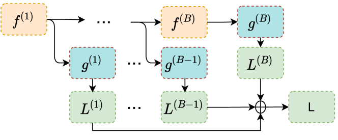
Figure 1: Training with early exits. Each exit branch $g^{(i)}$ propagates the prediction error in relation to the ground truth label $L^{(i)}$, training the blocks that precede each exit point $f^{(i-1)}$ for $i=1,\dots,B$.

This procedure allows for an efficient training of the whole ensemble in one go. Furthermore, differently from traditional deep ensembles using varying architectures, EEs as an ensemble allow for the earlier exits to incorporate feature learnt from the exits that follow.

3.3 Inference and predictive uncertainty

During inference, a single forward pass of the network produces a sequence of predictions, each potentially more accurate than the previous one. The overall prediction of the ensemble can be computed as the mean of a categorical distribution obtained from aggregating the predictions from the individual exits

$$p(\mathbf{y}_{1:T}|\mathbf{x}_{1:T})\approx\frac{1}{B}\sum_{i=1}^{B}\text{Softmax}(\hat{\mathbf{y}}^{(i)}_{1:T})$$ (4)

where the softmax function is applied time pointwise. Although the softmax function scales inputs to the range $[0,1]$, it is not a valid measure of probability since it is based on a point estimate. In contrast, as shown in Equation 7 (Appendix High Frequency EEG Artifact Detection with Uncertainty via Early Exit Paradigm), using our framework, real probability can be approximated from $B$ different possible outcomes from a single underlying data generating process.

Given the approximate distribution in Equation 7 (Appendix High Frequency EEG Artifact Detection with Uncertainty via Early Exit Paradigm), E⁴G can therefore capture predictive uncertainty as measured by metrics such as entropy:

$$H(\mathbf{y}_{1:T}|\mathbf{x}_{1:T})=-\sum_{\mathbf{y}_{1:T}\in\{0,1\}}p(\mathbf{y}_{1:T}|\mathbf{x}_{1:T})\log p(\mathbf{y}_{1:T}|\mathbf{x}_{1:T}).$$ (5)

Predictive uncertainty metrics give an interpretation of model decisions that can inform post-processing heuristics which would allow for the isolation highly uncertain predictions for further investigation by a human expert, thereby, increasing the overall trust and accuracy of the model.

4 Experiments

4.1 Dataset

We evaluate our framework on the Temple University EEG Artifact Corpus (v2.0) (TUH-A)  (Hamid et al., 2020). The dataset is composed of real EEG signals from 213 patients contaminated with artifacts which are human expert annotated. The artifacts range from chewing, eye movement, muscular movement, shivering and electrode errors. To best of our knowledge, we are the first to use this dataset in an automatic artifact detection framework. Appendix A contains further details on the dataset and preprocessing.

4.2 Implementation

For E⁴G , the backbone neural network $f_{\theta}(\cdot)$ is implemented as a temporal U-Net (Perslev et al., 2021), a fully convolutional encoder-decoder architecture for time series segmentation. We place exit blocks $g_{\phi_{i}}(\cdot)$ after each decoder block resulting in 4 predictions plus the output layer making a ensemble of $B=5$ as depicted in Figure 2. The ensemble size is in line with previous work suggesting the optimal number of samples needed for well calibrated uncertainty (Ovadia et al., 2019; Qendro et al., 2021a, b).

We compare E⁴G with two baselines both using the same backbone architecture. The first is a vanilla U-Net with no early exits and the second adds dropout at the end of each decoder block with a probability of $p=0.2$. The latter model is used for Monte Carlo dropout (MCDrop) (Gal & Ghahramani, 2015) based on 5 forward passes during testing.

For training, we use a joint loss composed of an equally weighted cross entropy loss and dice loss (Taghanaki et al., 2019; Isensee et al., 2019). All exits are considered as equally important by setting $\alpha_{i}=1$. We train all models for a maximum of 200 epochs with a batch size of 50 using the Adam optimizer (Kingma & Ba, 2014) with a learning rate of 1$e$-3. To prevent overfitting, model training was stopping based on no improvement in validation F1 score. All experiments are performed in PyTorch (Paszke et al., 2019). More details about model implementation can be found in Table 2 in Appendix B.

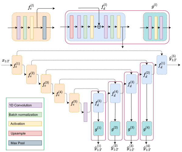
Figure 2: Overview of E⁴G based on a U-Net. The neural networks $f_{e}$, $f_{d}$, and $g$ represent the encoder, decoder and exit blocks, respectively (top). Each block in the encoder-decoder is connected by skip connections which perform feature concatenation (bottom). Exit blocks are placed after each hidden decoder block.

2*Model	2*F1 Score $\uparrow$	2*Precision $\uparrow$	2*Recall $\uparrow$	Predictive Entropy		Brier Score		Predictive Confidence
				True $\downarrow$	False $\uparrow$	True $\downarrow$	False $\uparrow$	True $\uparrow$	False $\downarrow$
Vanilla U-Net	0.840$\pm$.06	0.854$\pm$.03	0.832$\pm$.11	–	–	–	–	–	–
MCDrop U-Net	0.813$\pm$.07	0.821$\pm$.04	0.807$\pm$.10	0.243$\pm$.01	0.457$\pm$.01	0.023$\pm$.00	0.528$\pm$.01	0.905$\pm$.00	0.222$\pm$.01
Early Exit EEG (E4G )	0.838$\pm$.06	0.853$\pm$.03	0.829$\pm$.11	0.278$\pm$.01	0.531$\pm$.01	0.030$\pm$.001	0.547$\pm$.01	0.886$\pm$.01	0.274$\pm$.01

Table 1: Classification results and uncertainty metrics for EEG artifact detection on TUH-A. Reported results are the mean and standard deviation across 5 runs, each with a different random seed. The best results correspond to low uncertainty for true (right) predictions ($\downarrow$) and high uncertainty for false (wrong) predictions ($\uparrow$).

4.3 Results

Table 1 presents results for the task of per time point EEG artifact detection on the TUH-A test dataset. In addition to standard classification metrics, we consider Brier score, predictive confidence and predictive entropy as measures of uncertainty (see Appendix C.1 for a detailed description).

From the results it is clear that training with EEs does not degrade F1 score compared to the vanilla baseline (83.8% vs 84%). Instead, activating dropout during inference in MCDrop lowers F1 score by $~{}3\%$, suggesting a higher number of samples is required at test time to compensate for the dropped weights during inference. Already, by considering only 5 samples MCDrop increases latency by 5.2x compared to the vanilla baseline, while E⁴G increases latency only marginally (by only 1.1x). 

Importantly, E⁴G can provide well calibrated uncertainty that is better or comparable to MCDrop, especially for incorrect predictions as measured by predictive entropy (0.45 vs 0.53) and Brier score (0.53 vs 0.55), without incurring the computation overhead of the latter framework. Particularly within a medical setting, a highly uncertain false prediction, like the one provided by E⁴G , is more informative for a clinician-in-the-loop framework, where uncertain samples could be transferred to a human expert for further investigation (Leibig et al., 2017).

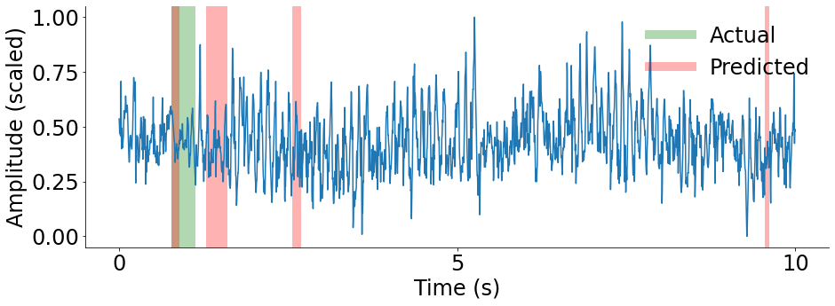
(a) Eye movement, exit 1

(b) Muscle movement, exit 1

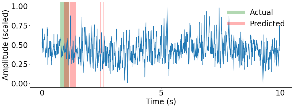
(c) Eye movement, exit 5

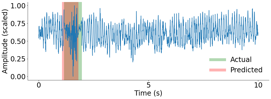
(d) Muscle movement, exit 5

Figure 3: Per time point EEG artifact predictions for Exits 1 and 5 within a 10 second window. Figure (a) and (c) show disagreement on how the artifact is distributed across time. Figure (b) and (d) show exit disagreement on the start and end point of the artifact. [Green = Actual, Red = Predicted, Brown = True prediction (Red + Green)]

4.4 Recommendations for using predictive uncertainty

Analyzing the results of the individual exits from E⁴G allows for uncertainty-informed decision making. Figure 3(a) and Figure 3(c) show an example for an eye movement artifact on a 10 second window. The two exits clearly disagree since their predictions (red sections) highlight the presence of the artifact in contradicting areas, particularly for the time points furthest away from the true occurrence of the artifact. Given high uncertainty of a false prediction, an automatic recommendation can be made for an expert clinician to review the sample (García Rodríguez et al., 2020; Xia et al., 2021).

On the other hand, Figure 3(b) and 3(d) show an example where the two exits agree over when the majority of a muscle movement artifact occur (brown sections). However, uncertainty is still apparent over the start and end time of the artifact. This is valuable information that can be used to automatically detect artifact boundaries for downstream removal and interpolation (Yang et al., 2018).

Although we only show two of the exits, Table 3 in Appendix C.2 shows results for all exits in the ensemble as well as examples of more artifacts. The strength of our framework is in exploiting exit predictive diversity for better performance and interpretability through the use of different ensemble aggregating strategies such as majority voting, model averaging and automatic thresholding which we leave for future work.

5 Conclusion

We introduce a general framework for enabling uncertainty quantification in any feed-forward deep neural network via the EE paradigm. Using the largest publicly available EEG artifact dataset, we evaluate our approach on the task of artifact detection and demonstrate how uncertainty, via E⁴G , can be used to inform decision making. Compared to the commonly used method of uncertainty quantification, Monte Carlo dropout (MCDrop), E⁴G performs better in terms of F1 score while providing comparable well-calibrated uncertainties in a single forward pass. In addition, unlike MCDrop our framework has access to uncertainty within the ensemble during training. Other methods that incorporate this functionality tend only to be pure Bayesian approaches that struggle with underfitting at scale and parameter efficiency (Dusenberry et al., 2020). Future work will include applying the EE paradigm to other architectures as well as other medical datasets like electronic health records. We envision extending our framework to exploit the uncertainty during training for adaptive decision making on joint tasks such as interpolation.

6 Acknowledgments

This work is supported by Nokia Bell Labs through their donation for the Centre of Mobile, Wearable Systems and Augmented Intelligence, ERC Project 833296 (EAR), as well as The Alan Turing Institute under the EPSRC grant EP/N510129/1.

Appendix A Dataset

From the TUH-A dataset, a common set of 21 EEG channels were retained from all patients and signals were resampled to the majority sampling frequency of $250$ Hz. Furthermore, all EEG signals were bandpass filtered (0.3-40 Hz) using a second-degree Butterworth filter and notch filtered at the power lower frequency 60 Hz similar to previous work (Svantesson et al., 2021). Finally, segments of clean and artifact samples of length 10s were created based on an analysis of the duration of the majority of artifacts. We treat each channel independently resulting in each sample $\mathbf{x}_{1:T}$ having size $M$=1 and $T$=2,500.

Since the dataset’s artifact classes are highly imbalanced, we augment the data by performing temporal window shifting and signal mixing (Cheng et al., 2020; Chiu et al., 2020) making sure not to mix signals from different EEG channels and patients. From the augmented dataset of 24,000 samples, we construct masks over time which act as a per time point labels specifying either the presence of an artifact, $y_{t}=1$ or clean signal $y_{t}=0$. Finally, we split the data into 80%, training, 10% validation and 10% testing keeping patient independent between datasets.

Appendix B Implementation

The core model was based on a temporal U-Net suggested by Perslev et al. (2021). Table 2 contains model implementation details.

Encoder Block		Decoder Block		Exit Block
Layer	Output	Layer	Output	Layer	Output
Conv1D, BN, ELU	5 x 2500	Upsample	22 x 156	Upsample	16 x 2500
Max Pool	5 x 1250	Conv1D, BN, ELU	16 x 156	Conv1D	2 x 2500
		Concatenate	32 x 156
		Conv1D, BN, ELU	16 x 156
Conv1D, BN, ELU	7 x 1250	Upsample	16 x 312	Upsample	12 x 2500
Max Pool	7 x 625	Conv1D, BN, ELU	12 x 312	Conv1D	2 x 2500
		Concatenate	24 x 312
		Conv1D, BN, ELU	12 x312
Conv1D, BN, ELU	9 x 625	Upsample	12 x 625	Upsample	9 x 2500
Max Pool	9 x 312	Conv1D, BN, ELU	9 x 625	Conv1D	2 x 2500
		Concatenate	18 x 625
		Conv1D, BN, ELU	9 x 625
Conv1D, BN, ELU	12 x 312	Upsample	9 x 1250	Upsample	7 x 2500
Max Pool	12 x 156	Conv1D, BN, ELU	7 x 1250	Conv1D	2 x 2500
		Concatenate	14 x1250
		Conv1D, BN, ELU	7 x 1250
Conv1D, BN, ELU	16 x 156	Upsample	7 x 2500
Max Pool	16 x 78	Conv1D, BN, ELU	5 x 2500
		Concatenate	10 x 2500
		Conv1D, BN, ELU	5 x 2500
Conv1D, BN, ELU	22 x 78	Conv1D, ELU	5 x 2500
		Conv1D	2 x 2500

Table 2: Implementation details of E⁴G . Shapes are based on an input size of $M=1$ and $T=2500$. [Max Pool = Max pooling with kernel size 2 and stride 1, Upsample = nearest-neighbor interpolation, Conv1D = 1D convolution with kernel size 4, stride 1, BN = Batch normalization, ELU = ELU activation function].

Appendix C Results

C.1 Uncertainty metrics

Let $\mathbf{y}_{1:T}=\{\mathbf{y}_{1},\dots,\mathbf{y}_{T}\}$ where each $\mathbf{y}_{t}\in\{0,1\}^{C}$ denote the true per time point class labels and $\mathbf{\hat{y}}_{1:T}$ where each $\mathbf{\hat{y}}_{t}\in\mathbb{R}^{C}$ denote the predicted per class and time point logits.

Brier score

is a measure of the accuracy of predicted probabilities. The Brier score for a single sample is defined

$$BS=\frac{1}{T}\sum_{t=1}^{T}(\bar{\mathbf{y}}_{t}-\mathbf{y}_{t})^{2}\\$$ (6)

where $\bar{\mathbf{y}}_{t}=\frac{1}{B}\sum_{i=1}^{B}\text{Softmax}(\mathbf{\hat{y}}^{(i)}_{t})$ is the average vector of class probabilities over all exits for a given time point.

Predictive confidence

measures the largest predicted class probability. Predictive confidence is defined as

$$PC=\frac{1}{T}\sum_{t=1}^{T}\text{max}(\bar{\mathbf{y}}_{t}).$$ (7)

Predictive entropy

measure the average amount of information in the predicted distribution. Predictive entropy is defined in Equation 5.

C.2 Model predictions

Table 3 shows example results of per exit artifact predictions on the test dataset. The first two artifacts refer to Figure 3 whilst the second two rows refer to Figure 4.

2*Artifact	F1 Score $\uparrow$
	Exit 1	Exit 2	Exit 3	Exit 4	Exit 5
Eye movement	0.60	0.71	0.73	0.73	0.74
Muscle movement	0.99	0.96	0.92	0.92	0.94
Electrode	0.92	0.78	0.84	0.84	0.84
Chewing	0.70	0.71	0.79	0.81	0.79

Table 3: Average per time point F1 scores of artifact predictions across each exit. Highly disagreeing exits have a larger difference in F1 score.

Estimating uncertainty helps in isolating cases where the model is guessing at random as we can see from the predictions further from the occurrence of the true chewing artifact in Figure 4(a) and 4(c). Figure 4(b) and 4(d) show an electrode artifact where the model is more accurate at exit 1 (0.92) compared to later exits (0.84¡) demonstrating that later exits in the ensemble are not always better at making correct predictions. Exit 4 predicts a longer time frame for the artifact occurrence reflecting greater uncertainty.

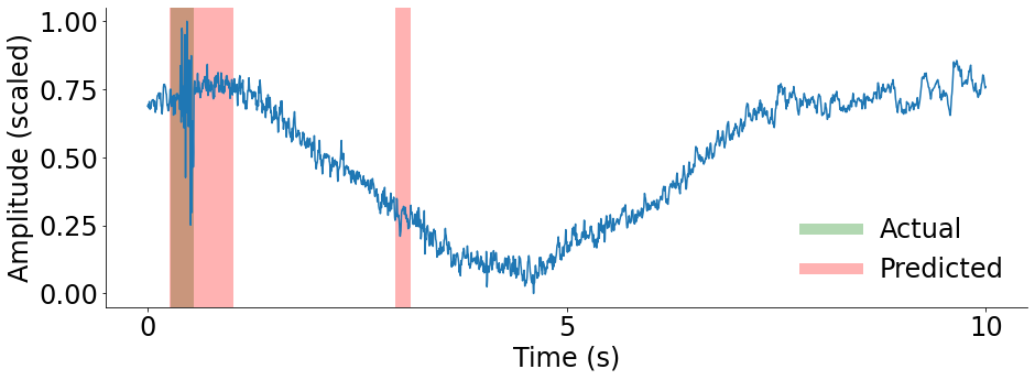
(a) Chewing, exit 1

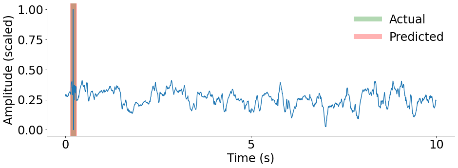
(b) Electrode, exit 1

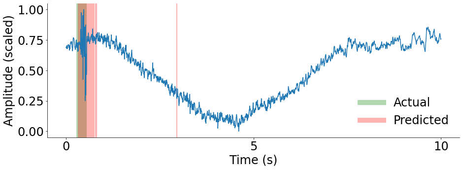
(c) Chewing, exit 5

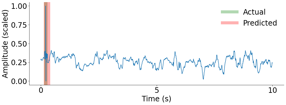
(d) Electrode, exit 5

Figure 4: Per time point EEG artifact predictions for Exits 1 and 5 within a 10 second window. Figure (a) and (c) show disagreement on how the artifact is distributed across time. Figure (b) and (d) show exit disagreement on the end point of the artifact. [Green = Actual, Red = Predicted, Brown = True prediction (Red + Green)]

References

- Acharya et al. (2013) Acharya, U. R., Sree, S. V., Swapna, G., Martis, R. J., and Suri, J. S. Automated eeg analysis of epilepsy: a review. Knowledge-Based Systems, 45:147–165, 2013.
- Bolukbasi et al. (2017) Bolukbasi, T., Wang, J., Dekel, O., and Saligrama, V. Adaptive neural networks for fast test-time prediction. arXiv preprint arXiv:1702.07811, 2017.
- Castellanos & Makarov (2006) Castellanos, N. P. and Makarov, V. A. Recovering eeg brain signals: artifact suppression with wavelet enhanced independent component analysis. Journal of neuroscience methods, 158(2):300–312, 2006.
- Cheng et al. (2020) Cheng, J. Y., Goh, H., Dogrusoz, K., Tuzel, O., and Azemi, E. Subject-aware contrastive learning for biosignals. arXiv preprint arXiv:2007.04871, 2020.
- Chiu et al. (2020) Chiu, C.-Y., Hsiao, W.-Y., Yeh, Y.-C., Yang, Y.-H., and Su, A. W.-Y. Mixing-specific data augmentation techniques for improved blind violin/piano source separation. In 2020 IEEE 22nd International Workshop on Multimedia Signal Processing (MMSP), pp. 1–6. IEEE, 2020.
- Cisotto et al. (2020) Cisotto, G., Zanga, A., Chlebus, J., Zoppis, I., Manzoni, S., and Markowska-Kaczmar, U. Comparison of attention-based deep learning models for eeg classification. arXiv preprint arXiv:2012.01074, 2020.
- de Aguiar Neto & Rosa (2019) de Aguiar Neto, F. S. and Rosa, J. L. G. Depression biomarkers using non-invasive eeg: A review. Neuroscience & Biobehavioral Reviews, 105:83–93, 2019.
- Dusenberry et al. (2020) Dusenberry, M., Jerfel, G., Wen, Y., Ma, Y., Snoek, J., Heller, K., Lakshminarayanan, B., and Tran, D. Efficient and scalable bayesian neural nets with rank-1 factors. In International conference on machine learning, pp. 2782–2792. PMLR, 2020.
- Gal & Ghahramani (2015) Gal, Y. and Ghahramani, Z. Bayesian convolutional neural networks with bernoulli approximate variational inference. arXiv preprint arXiv:1506.02158, 2015.
- Gal & Ghahramani (2016) Gal, Y. and Ghahramani, Z. Dropout as a bayesian approximation: Representing model uncertainty in deep learning. In international conference on machine learning, pp. 1050–1059, 2016.
- García Rodríguez et al. (2020) García Rodríguez, C., Vitrià, J., and Mora, O. Uncertainty-based human-in-the-loop deep learning for land cover segmentation. Remote Sensing, 12(22):3836, 2020.
- Hamid et al. (2020) Hamid, A., Gagliano, K., Rahman, S., Tulin, N., Tchiong, V., Obeid, I., and Picone, J. The temple university artifact corpus: An annotated corpus of eeg artifacts. In 2020 IEEE Signal Processing in Medicine and Biology Symposium (SPMB), pp. 1–4. IEEE, 2020.
- Hazra et al. (2010) Hazra, B., Roffel, A., Narasimhan, S., and Pandey, M. Modified cross-correlation method for the blind identification of structures. Journal of Engineering Mechanics, 136(7):889–897, 2010.
- Hu et al. (2015) Hu, J., Wang, C.-s., Wu, M., Du, Y.-x., He, Y., and She, J. Removal of eog and emg artifacts from eeg using combination of functional link neural network and adaptive neural fuzzy inference system. Neurocomputing, 151:278–287, 2015.
- Huang et al. (2017) Huang, G., Chen, D., Li, T., Wu, F., van der Maaten, L., and Weinberger, K. Q. Multi-scale dense networks for resource efficient image classification. arXiv preprint arXiv:1703.09844, 2017.
- Isensee et al. (2019) Isensee, F., Petersen, J., Kohl, S. A., Jäger, P. F., and Maier-Hein, K. H. nnu-net: Breaking the spell on successful medical image segmentation. arXiv preprint arXiv:1904.08128, 1:1–8, 2019.
- Jafari et al. (2017) Jafari, A., Gandhi, S., Konuru, S. H., Hairston, W. D., Oates, T., and Mohsenin, T. An eeg artifact identification embedded system using ica and multi-instance learning. In 2017 IEEE International Symposium on Circuits and Systems (ISCAS), pp. 1–4. IEEE, 2017.
- Khatwani et al. (2021) Khatwani, M., Rashid, H.-A., Paneliya, H., Horton, M., Waytowich, N., Hairston, W. D., and Mohsenin, T. A flexible multichannel eeg artifact identification processor using depthwise-separable convolutional neural networks. ACM Journal on Emerging Technologies in Computing Systems (JETC), 17(2):1–21, 2021.
- Kingma & Ba (2014) Kingma, D. P. and Ba, J. Adam: A method for stochastic optimization. arXiv preprint arXiv:1412.6980, 2014.
- Lee et al. (2020) Lee, S. S., Lee, K., and Kang, G. Eeg artifact removal by bayesian deep learning & ica. In 2020 42nd Annual International Conference of the IEEE Engineering in Medicine & Biology Society (EMBC), pp. 932–935. IEEE, 2020.
- Leibig et al. (2017) Leibig, C., Allken, V., Ayhan, M. S., Berens, P., and Wahl, S. Leveraging uncertainty information from deep neural networks for disease detection. Scientific reports, 7(1):1–14, 2017.
- Leite et al. (2018) Leite, N. M. N., Pereira, E. T., Gurjão, E. C., and Veloso, L. R. Deep convolutional autoencoder for eeg noise filtering. In 2018 IEEE International Conference on Bioinformatics and Biomedicine (BIBM), pp. 2605–2612. IEEE, 2018.
- Montanari et al. (2020) Montanari, A., Sharma, M., Jenkus, D., Alloulah, M., Qendro, L., and Kawsar, F. eperceptive: energy reactive embedded intelligence for batteryless sensors. In Proceedings of the 18th Conference on Embedded Networked Sensor Systems, pp. 382–394, 2020.
- Mowla et al. (2015) Mowla, M. R., Ng, S.-C., Zilany, M. S., and Paramesran, R. Artifacts-matched blind source separation and wavelet transform for multichannel eeg denoising. Biomedical Signal Processing and Control, 22:111–118, 2015.
- Ochal et al. (2020) Ochal, D., Rahman, S., Ferrell, S., Elseify, T., Obeid, I., and Picone, J. The temple university hospital eeg corpus: Annotation guidelines. Institute for Signal and Information Processing Report, 1(1), 2020.
- Ovadia et al. (2019) Ovadia, Y., Fertig, E., Ren, J., Nado, Z., Sculley, D., Nowozin, S., Dillon, J. V., Lakshminarayanan, B., and Snoek, J. Can you trust your model’s uncertainty? evaluating predictive uncertainty under dataset shift. arXiv preprint arXiv:1906.02530, 2019.
- Paszke et al. (2019) Paszke, A., Gross, S., Massa, F., Lerer, A., Bradbury, J., Chanan, G., Killeen, T., Lin, Z., Gimelshein, N., Antiga, L., et al. Pytorch: An imperative style, high-performance deep learning library. arXiv preprint arXiv:1912.01703, 2019.
- Perslev et al. (2019) Perslev, M., Jensen, M. H., Darkner, S., Jennum, P. J., and Igel, C. U-time: A fully convolutional network for time series segmentation applied to sleep staging. arXiv preprint arXiv:1910.11162, 2019.
- Perslev et al. (2021) Perslev, M., Darkner, S., Kempfner, L., Nikolic, M., Jennum, P. J., and Igel, C. U-sleep: resilient high-frequency sleep staging. NPJ digital medicine, 4(1):1–12, 2021.
- Qendro et al. (2021a) Qendro, L., Chauhan, J., Ramos, A. G. C., and Mascolo, C. The benefit of the doubt: Uncertainty aware sensing for edge computing platforms. arXiv preprint arXiv:2102.05956, 2021a.
- Qendro et al. (2021b) Qendro, L., Ha, S., de Jong, R., and Maji, P. Stochastic-shield: A probabilistic approach towards training-free adversarial defense in quantized cnns. arXiv preprint arXiv:2105.06512, 2021b.
- Ronneberger et al. (2015) Ronneberger, O., Fischer, P., and Brox, T. U-net: Convolutional networks for biomedical image segmentation. In International Conference on Medical image computing and computer-assisted intervention, pp. 234–241. Springer, 2015.
- Scardapane et al. (2020) Scardapane, S., Scarpiniti, M., Baccarelli, E., and Uncini, A. Why should we add early exits to neural networks? Cognitive Computation, 12(5):954–966, 2020.
- Seifzadeh et al. (2014) Seifzadeh, S., Faez, K., and Amiri, M. Comparison of different linear filter design methods for handling ocular artifacts in brain computer interface system. Journal of Computer & Robotics, 7(1):51–56, 2014.
- Shahzad & Lavesson (2013) Shahzad, R. K. and Lavesson, N. Comparative analysis of voting schemes for ensemble-based malware detection. Journal of Wireless Mobile Networks, Ubiquitous Computing, and Dependable Applications, 4(1):98–117, 2013.
- Svantesson et al. (2021) Svantesson, M., Olausson, H., Eklund, A., and Thordstein, M. Virtual eeg-electrodes: Convolutional neural networks as a method for upsampling or restoring channels. Journal of Neuroscience Methods, 355:109126, 2021.
- Taghanaki et al. (2019) Taghanaki, S. A., Zheng, Y., Zhou, S. K., Georgescu, B., Sharma, P., Xu, D., Comaniciu, D., and Hamarneh, G. Combo loss: Handling input and output imbalance in multi-organ segmentation. Computerized Medical Imaging and Graphics, 75:24–33, 2019.
- Winkler et al. (2014) Winkler, I., Brandl, S., Horn, F., Waldburger, E., Allefeld, C., and Tangermann, M. Robust artifactual independent component classification for bci practitioners. Journal of neural engineering, 11(3):035013, 2014.
- Xia et al. (2021) Xia, T., Han, J., Qendro, L., Dang, T., and Mascolo, C. Uncertainty-aware covid-19 detection from imbalanced sound data. arXiv preprint arXiv:2104.02005, 2021.
- Yang et al. (2018) Yang, B., Duan, K., Fan, C., Hu, C., and Wang, J. Automatic ocular artifacts removal in eeg using deep learning. Biomedical Signal Processing and Control, 43:148–158, 2018.