Multi-critical point principle as the origin of classical conformality and its generalizations

Abstract

Multi-critical point principle (MPP) is one of the interesting theoretical possibilities that can explain the fine-tuning problems of the Universe. It simply claims that “the coupling constants of a theory are tuned to one of the multi-critical points, where some of the extrema of the effective potential are degenerate.” One of the simplest examples is the vanishing of the second derivative of the effective potential around a minimum. This corresponds to the so-called classical conformality, because it implies that the renormalized mass $m^{2}$ vanishes. More generally, the form of the effective potential of a model depends on several coupling constants, and we should sweep them to find all the multi-critical points. In this paper, we study the multi-critical points of a general scalar field $\phi$ at one-loop level under the circumstance that the vacuum expectation values of the other fields are all zero. For simplicity, we also assume that the other fields are either massless or so heavy that they do not contribute to the low energy effective potential of $\phi$. This assumption makes our discussion very simple because the resultant one-loop effective potential is parametrized by only four effective couplings. Although our analysis is not completely general because of the assumption, it still can be widely applicable to many models of the Coleman-Weinberg mechanism and its generalizations. After classifying the multi-critical points at low-energy scales, we will briefly mention the possibility of criticalities at high-energy scales and their implications for cosmology.

1 Introduction

For the last few decades, the Standard Model (SM) has been tested by various experiments and observations, but any significant clues to new physics have not been discovered yet. Moreover, the renormalization group (RG) analysis based on the observed SM parameters supports the hypothesis that the SM is not much altered up to the Planck scale  [1, 2, 3, 4, 5, 6], which strongly suggests a possibility of “desert scenario” such that the SM might be directly connected to an ultraviolet complete theory.

On the other hand, it is also true that there are a lot of mysteries and problems in particle physics and cosmology: For example, why is the the electroweak (EW) scale $v=246$ GeV so small compared to the Planck scale $10^{18}$ GeV ? Why is the vacuum energy of the present universe so tiny ? Why are there huge mass hierarchies among the SM fermions ? Why are there three generations ? What is dark matter ? What is the origin of baryon asymmetry of the universe ? etc. Though we can easily make an extended model of the SM to explain some phenomenological aspects such as dark matter or baryon asymmetry, other issues related to the naturalness seem to require more radical and fundamental approaches than the ordinary quantum field theory.

The various observations of the SM may already provide important hints for solving these naturalness problems. It is a well-known fact that the Higgs potential becomes negatively large below the Planck scale when the top-quark mass is larger than some value. More precisely, the critical value of the top-quark pole mass for the theoretical border between stability and instability of the SM vacuum is $m_{t,\text{critical}}^{\rm pole}\simeq 171.4$ GeV [7, 8], which is consistent at the 1.4 $\sigma$ level with the latest combination of the experimental results $m_{t}^{\rm pole}=172.4\pm 0.7$ GeV [9]. Surprisingly, for the critical top mass, the vacuum expectation value of the Higgs field is nearly equal to the Planck scale, and such a behavior of the potential has a lot of implications to high energy physics and cosmology. This interesting behavior of the Higgs potential can be understood as one of the manifestations of the multi-critical point principle (MPP) [10, 11, 12, 13, 14, 15, 16, 17, 18, 19, 20]. Actually there are several manners to represent the MPP. A simple one is: “The coupling constants of a theory are tuned to one of the multi-critical points of the vacua. In other words, some of the extrema of the effective potential should be degenerate.” In this sense, the MPP provides a natural fine-tuning mechanism for coupling constants in quantum field theory.

Note that the effective potential exists independently of the renormalization scale, up to the wave function renormalization of the field, for a given set of bare parameters. In general, when there is only one mass scale involved, we can approximate the effective potential by lower order perturbations by choosing the renormalisation scale around that mass scale. In this paper, we discuss that non-trivial critical points exist near the mass scale where the running quartic coupling becomes zero.

Here we give a short introduction to the MPP to clarify and visualize how the renormalized parameters are fixed by this principle. For simplicity, let us consider the effective potential $V(\phi)$ of a general scalar field $\phi$. In general $V(\phi)$ depends on the coupling constants $\{m^{2},~{}\lambda,~{}g,~{}y,\cdots\}$ of the theory, and its extrema change as we vary them. Then, we can find critical points in the parameter space at which some of the extrema become degenerate. As we see below, the multiplicity of a criticality is equal to the number of fine tunings to reach it.

The generic criticality is the degeneracy of two extrema, which can be classified into two cases. One is that two non-adjacent extrema are degenerate. (See the upper-left panel in Fig. 1 for example.) The other is that two adjacent local minimum and local maximum degenerate to form a saddle point. (See the upper-right panel in Fig. 1.) In either cases, the criticality is obtained when one equation is satisfied, that is, $V|_{\phi=\phi_{1}}=V|_{\phi=\phi_{2}}$ for the former or $V^{\prime}|_{\phi=\phi_{s}}=V^{\prime\prime}|_{\phi=\phi_{s}}=0$ for the latter case. Therefore the generic criticality is reached by one-parameter tuning.

We can also consider multiple criticalities that correspond to multi-parameter tunings. The lower two panels in Fig. 1 show examples of the doubly critical points. The lower-left panel shows a double criticality where a local minimum (false vacuum) degenerates with a saddle point, while in the lower-right panel there are two saddle points. It is easy to check that they are obtained by tuning two parameters.

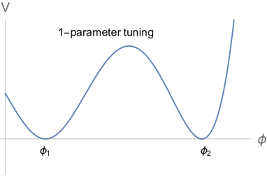
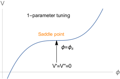
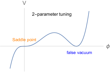
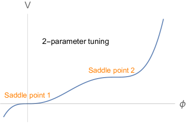
Figure 1: Typical examples of the MPP. The upper panels correspond to 1-parameter tuning while the lower panels correspond to 2-parameter tuning.

In general, there are a number of multiple critical points in the (one-loop) effective potential. The most important of these is the point with the highest criticality. This is because they are the most likely to occur according to the MPP. These critical points are called “maximally critical points”. As we will explain, one of them corresponds to the the classical conformality (CC) assumption [21, 22, 23, 24, 25, 26, 27, 28, 29, 30, 31, 32, 33, 34, 35], that leads to the Coleman-Weinberg (CW) potential. However, from the MPP point of view, all the maximally critical points are equally important, and the CW potential should have several variations corresponding to them.

The ultimate goal is to classify the maximally critical points of general theory. If we restrict the problem to one-loop, we can write down the general form of the effective potential (see Eq. (1)). However the systematic search for the multi-critical points of such a potential is still too complicated a problem. Here, we will simply assume that the vacuum expectation values of all the fields except the field $\phi$ are zero. Furthermore, we assume that the other fields are either massless or so heavy that they do not contribute to the low energy effective potential of $\phi$. We can imagine that the masslessness of the other fields appears as a consequence of the MPP as in the case of the CC. Thanks to these assumptions, the one-loop effective potential can be expressed by four parameters (see Eq. (16)), and we can study the maximally critical points in a model-independent manner. The study of doubly critical points corresponding to two-parameter tunings is also presented in Appendix A. Although the effective potential we consider here is rather restricted, the result can be used to analyze various models of the modification of the SM. At any rate, the main purpose of this paper is to give general idea and philosophy of the MPP so that readers can use it when studying a concrete model of particle physics.

In general, the effective potential can also have another vacuum or saddle point at high energy scale due to the RG running effects as in the case of the Higgs potential. We will also briefly mention this possibility and its possible implications for cosmology. See Refs. [7, 36, 37, 38, 39, 40, 41] and references therein for more details.

The organization of the paper is as follows. In Sec. 2, we review one-loop effective potential. In Sec. 3, we classify the maximally critical points of the above mentioned effective potential. Summary and discussion are given in Sec. 4. In Appendix A, we discuss doubly critical points.

2 One-loop effective potential

In this section, we discuss the one-loop effective potential of a general scalar field $\phi$. In a mass independent renormalization scheme, the renormalized one-loop effective potential is generally given by

$$V(\phi,\lambda_{a},m^{2};\mu)=\lambda_{1}\phi+\frac{m^{2}}{2}\phi^{2}+\frac{\lambda_{3}}{3!}\phi^{3}+\frac{\lambda_{\phi}}{4!}\phi^{4}+\sum_{i}n_{i}(-1)^{2s_{i}}\frac{M_{i}(\phi)^{4}}{64\pi^{2}}\ln\left(\frac{M_{i}(\phi)^{2}}{\mu^{2}e^{C_{i}}}\right)~{},$$ (1)

where $s_{i}$ and $n_{i}$ represent the spin and the number of degrees of freedom (dof) of particle species $i$, respectively, $M_{i}(\phi)$ is the background-dependent mass, and $\mu e^{C_{i}/2}$ is the renormalization scale with $C_{i}$ being the scheme dependent constant. The renormalization-scale independence of the effective potential is expressed as

$${\cal D}V(\phi;\mu) :=\frac{d}{d\ln\mu}V(\phi;\mu)$$

$$=\left(\mu\frac{\partial}{\partial\mu}+\sum_{a}\beta_{\lambda_{a}}\frac{\partial}{\partial\lambda_{a}}-\gamma_{m}m^{2}\frac{\partial}{\partial m^{2}}-\gamma_{\phi}\phi\frac{\partial}{\partial\phi}\right)V(\phi;\mu)=0~{},$$ (2)

where $\lambda_{a}$ and $\beta_{\lambda_{a}}$ denote a general coupling constant and its beta function, and $\gamma_{\phi}$ is the wave function renormalization. The solution of this partial differential equation is [42]

$$V(\phi,\lambda_{a},m^{2};\mu)=V(\overline{\phi},\overline{\lambda}_{a},\overline{m}^{2};\overline{\mu}=e^{t}\mu)~{},$$ (3)

where $\overline{\lambda}_{a}$, $\overline{m}^{2}$ and $\overline{\phi}$ are the running quantities;

$$\frac{d\overline{\lambda}_{a}}{dt}=\beta_{\lambda_{a}}(\{\overline{\lambda}_{a}\})~{},\quad\overline{\lambda}_{a}|_{\overline{\mu}=\mu}=\lambda_{a}~{},$$ (4)

$$\frac{d\overline{m}^{2}}{dt}=-\gamma_{m}\overline{m}^{2}~{},\quad\overline{m}^{2}|_{\overline{\mu}=\mu}=m^{2}~{},$$ (5)

$$\frac{d\overline{\phi}}{dt}=-\gamma_{\phi}\overline{\phi}~{},\quad\overline{\phi}|_{\overline{\mu}=\mu}=\phi~{}.$$ (6)

In the following, we will not put bars explicitly and interpret that all the quantities obey the above RGEs as we vary $\mu$.

It would be educational to revisit the Coleman-Weinberg (CW) mechanism here. (Note that this case corresponds to the criticality 234-15 in the next section. ) When a model has no dimensionfull parameters at tree level, the mass $M_{i}(\phi)$ is typically given by $M_{i}(\phi)=g_{i}\phi$ where $g_{i}$ denotes a coupling constant. Then, the one-loop effective potential becomes

$$V(\phi;\mu) =\frac{\lambda_{\phi}}{4!}\phi^{4}+\sum_{i}n_{i}(-1)^{2s_{i}}\frac{M_{i}(\phi)^{4}}{64\pi^{2}}\ln\left(\frac{M_{i}(\phi)^{2}}{\mu^{2}e^{C_{i}}}\right)$$ (7)

$$=\frac{\lambda_{\phi}+\delta\lambda_{\phi}}{4!}\phi^{4}+\frac{\beta_{\lambda_{\phi}}}{2\cdot 4!}\phi^{4}\log\left(\frac{\phi^{2}}{\mu^{2}}\right)~{},$$ (8)

where $\beta_{\lambda_{\phi}}$ is the one-loop beta function of $\lambda_{\phi}$ without the contributions from the wave function renormalization, and

$$\delta\lambda_{\phi}=\sum_{i}n_{i}(-1)^{2s_{i}}\frac{3g_{i}^{4}}{8\pi^{2}}\ln\left(g_{i}^{2}/e^{C_{i}}\right)~{}.$$ (9)

The easiest way to understand CW mechanism is to choose the renormalization scale as $\mu=M$ where $M$ is the scale at which $\lambda_{\phi}+\delta\lambda_{\phi}$ vanishes;

$$V(\phi;\mu=M)=\frac{\beta_{\lambda_{\phi}}}{2\cdot 4!}\phi^{4}\log\left(\frac{\phi^{2}}{M^{2}}\right)~{}.$$ (10)

This potential has a minimum at $\phi=Me^{-1/4}$, which induces a symmetry breaking. Note that if we impose the initial conditions of the RGEs at a high-energy scale $\Lambda$, $M$ is rougly given by

$$M\sim\Lambda\exp\left(-\lambda_{\phi}/\beta_{\lambda_{\phi}}\right)\bigg{|}_{\mu=\Lambda}~{},$$ (11)

which is a well-known result of dimensional transmutation.

As another choice of the renormalization scale, $\mu\sim\phi$ is also frequently used because it corresponds to the resummation of leading-log terms [42, 43]. In this case, the potential Eq. (8) becomes

$$V(\phi;\mu=\phi)=\frac{\lambda_{\phi}^{\rm eff}(\mu=\phi)}{4!}\phi^{4}~{},$$ (12)

where $\lambda_{\phi}^{\rm eff}:=\lambda_{\phi}+\delta\lambda_{\phi}$. This choice is particularly useful when we study large-field behaviors of the potential because no large logarithmic terms appear by definition. As a consistency check, it would be meaningful to reproduce the CW mechanism in this case: By assuming that $\lambda_{\rm eff}(\phi)$ becomes zero at $\phi=M$, $\lambda_{\phi}^{\rm eff}(\phi)$ can be approximately expanded as

$$\lambda_{\phi}^{\rm eff}(\phi)\sim 0+\frac{\beta_{\lambda_{\phi}}}{2}\log\left(\frac{\phi^{2}}{M^{2}}\right)$$ (13)

around $\phi=M$, and we can see that Eq. (12) is now identical to Eq. (10). This also confirms the renormalization-scale independence of the CW mechanism. In the following, we will mainly use $\mu=M$ since we are interested in the effective potential at low-energy scales.

3 Multi-critical points of one-loop effective potential

In this section, we study the critical behaviors of the one-loop effective potential Eq. (1). In a general gauge theory, in addition to $\phi$, we have other scalar field(s) $S$, gauge field(s) $A_{\mu}$, and fermion(s) $\psi$. Their masses that depend on the back-ground of $\phi$ are given by

$$M_{\phi}(\phi)^{2}=m^{2}+\lambda_{3}\phi+\lambda\phi^{2}/2~{},\ M_{S}(\phi)^{2}=m_{S}^{2}+\Lambda_{\phi S}\phi+\lambda_{\phi S}\phi^{2}/2~{},\ M_{A}(\phi)=g\phi~{},\ M_{\psi}(\phi)=m_{\psi}+y\phi~{},$$ (14)

respectively. Studying the critical behavior of Eq. (1) in this most general form is beyond the scope of this paper. Instead, we simply assume that only the $\phi$ sector has dimensionful parameters at tree level. Under this assumption, Eq. (14) are reduced to the form $M_{i}(\phi)=g_{i}\phi$ except for $M_{\phi}(\phi)$, and Eq. (1) can be written as

$$V(\phi;\mu)=\lambda_{1}\phi+\frac{m^{2}}{2}\phi^{2}+\frac{\lambda_{3}}{3!}\phi^{3}+\frac{\lambda_{\phi}^{\rm eff}}{4!}\phi^{4}+\frac{c}{2\cdot 4!}\phi^{4}\log\left(\frac{\phi^{2}}{\mu^{2}}\right)+\frac{M_{\phi}(\phi)^{4}}{64\pi^{2}}\log\left(\frac{M_{\phi}(\phi)^{2}}{\mu^{2}e^{3/2}}\right)~{},$$ (15)

where $c$ is a coefficient determined by the coupling constants of the model, and the last term denotes the one-loop contribution from $\phi$ itself. The basic assumption of MPP is that the super-renormalizable coupling constants are adjusted to one of the multi-critical points. Therefore, we regard $c$ as a constant. In the following, we will neglect the last term and discuss the multi-critical points by the first five terms. This simplification is justified in the following sense: $c$ is typically ${\cal O}(\lambda^{2},g^{4},y^{4})$, which is small as long as the model is perturbative. Then, the MPP fixes the remaining parameters $(\lambda_{1},m^{2},\lambda_{3})$ at small values $\sim c$, and this guarantees the smallness of the last term in Eq. (15) because $M_{\phi}(\phi)^{4}\sim c^{2}\phi^{4}$, which is suppressed by a factor $c$ compared to the first five terms around the critical points.

3.1 Multi-critical points at low-energy scale

Now let us investigate the critical behavior of Eq. (15) in the low-energy region. By “low-energy” here, we mean $\phi\sim M$ where $M$ is the CW scale where the effective quartic coupling $\lambda_{\phi}^{\rm eff}$ becomes zero. As in the case of the previous section, a simple way to study the effective potential around $\phi\sim M$ is to choose $\mu=M$. Then, we have

$$V(\phi;\mu=M) =\lambda_{1}\phi+\frac{m^{2}}{2}\phi^{2}+\frac{\lambda_{3}}{3!}\phi^{3}+\frac{c}{2\cdot 4!}\phi^{4}\log\left(\frac{\phi^{2}}{M^{2}}\right)~{},$$ (16)

where all the coupling constants are evaluated at $\mu=M$. Note that $c$ should be positive to ensure the stability of the potential.

Here we should mention the higher-loop corrections. The MPP predicts that the tree-level couplings $\lambda_{i}$ become the same order as $c$. Then, the two-loop corrections are typically ${\cal O}(\lambda_{i}^{3}/(16\pi^{2}))={\cal O}(c^{3}/(16\pi^{2}))\ll c$. Therefore, the critical points discussed in this paper are self-consistent in that the contributions of higher-loop corrections are negligible. More complicated critical points can appear when the tree-level couplings are of the same order as the coefficients of the higher-loop corrections. The study of such multi-critical points of general effective potentials is the next theoretical challenge.

In Eq. (16), the effective potential $V$ has five parameters $\lambda_{1}$, $m^{2}$, $\lambda_{3}$, $c$, $M$. However, an overall rescaling of $V$ or $\phi$ does not change the pattern of the degeneracy of extrema. Therefore, we can fix $c$ and $M$ to some arbitrary values, and then examine the criticality by changing the other three parameters, $\lambda_{1}$, $m^{2}$, $\lambda_{3}$. In other words, we consider criticality in the three dimensional parameter space. Therefore a triple criticality is the maximum for this effective potential.

Next we examine the extremum points of $V$. The derivatives of Eq. (16) are

$$\frac{\partial V}{\partial\phi} =\lambda_{1}+m^{2}\phi+\frac{\lambda_{3}}{2}\phi^{2}+\frac{c}{3!2}\phi^{3}\left[\ln\left(\frac{\phi^{2}}{M^{2}}\right)+\frac{1}{2}\right]~{},$$ (17)

$$\frac{\partial^{2}V}{\partial\phi^{2}} =m^{2}+\lambda_{3}\phi+\frac{c}{2!2}\phi^{2}\left[\ln\left(\frac{\phi^{2}}{M^{2}}\right)+\frac{7}{6}\right]~{},$$ (18)

$$\frac{\partial^{3}V}{\partial\phi^{3}} =\lambda_{3}+\frac{c}{2}\phi\left[\ln\left(\frac{\phi^{2}}{M^{2}}\right)+\frac{13}{6}\right]~{},$$ (19)

$$\frac{\partial^{4}V}{\partial\phi^{4}} =\frac{c}{2}\left[\ln\left(\frac{\phi^{2}}{M^{2}}\right)+\frac{25}{6}\right]~{}.$$ (20)

By integrating these derivatives step by step, it is easy to see that there are generically five extrema. These are named 1, 2, 3, 4, and 5 from left to right on the $\phi$ axis, respectively. Note that 1, 3, 5 are local minima, while 2, 4 are local maxima.

In the parameter space, for each pair of the extrema, there is a hypersurface on which those two extrema are degenerate. This corresponds to a criticality obtained by a one-parameter tuning, and we express such a criticality as $ab$, where $a$ and $b$ are the name of the extrema that degenerate. Note that the degeneracy between neighboring extrema (e.g. $12,~{}23,~{}\cdots$) corresponds to a saddle point.

In principle, one can think of multi-critical points as the intersection of such hypersurfaces. For higher critical points, however, it is easier to classify them in a combinatorial way. In fact, there are two categories of double critical points. In one category, three extrema $a$, $b$, and $c$ are degenerate, which is denoted as $abc$. In the other category, two pairs $(a,b)$ and $(c,d)$ are degenerate respectively, and it is denoted as $ab-cd$. Similarly, there are two categories of triple critical points. In one category, four extrema $a$, $b$, $c$, and $d$ are degenerate, which is denoted as $abcd$. In the other category, one triplet $(a,b,c)$ and one pair $(d,e)$ are each degenerate, which is denoted as $abc-de$. Note that a triple criticality consisting of three pairs like $ab-cd-ef$ does not exist in our case, because we have only five extremal points.

In the following, we will explicitly write down the form of the effective potential at multi-critical points. We represent the true vacuum (false vacuum) as $\phi=v_{\phi}~{}(v_{f})$, the saddle point as $\phi_{S}$, and the mass of $\phi$ at $\phi=v_{\phi}$ as $m_{\phi}$.

$\bullet$ Maximally critical points

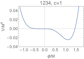
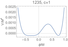
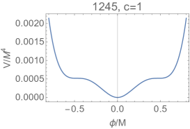
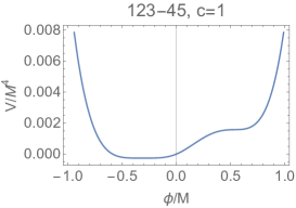
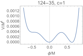
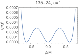
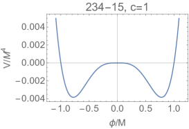
Figure 2: The effective potentials corresponding to the tricritical points. Here

Let us start with classifying the maximally critical points, that is, triple criticalities. First, we point out that there is no need to distinguish between two criticalities that can be transferred by reversing the sign of $\phi$. For example, $123-45$ and $543-21$ are considered to be the same. Then the possible patterns of degeneracies are

$$1234~{},\ 1235~{},\ 1245~{},$$

$$123-45~{},\ 124-35~{},\ 125-34~{},\ 134-25~{},\ 135-24~{},\ 234-15~{}.$$ (21)

In the second line, however, not all of them are realized, which can be seen as follows. For example, let’s take a look at $125-34$. Here, $V(a)$ denote the value of $V$ at the extremum $a$. Because $3$ is a neighbor of the local maximum $2$, we have $V(2)>V(3)$. Similarly, because $4$ is a neighbor of the local minimum $5$, we have $V(4)>V(5)$. On the other hand from the degeneracy pattern we have $V(2)=V(5)$ and $V(3)=V(4)$, which contradict with the above inequalities. Similarly, $134-25$ is not realized.

Thus, we find that there are seven triple critical points. As we have discussed, each of them needs a three-parameter tuning, and the effective potential is completely fixed up to overall rescalings of $V$ and $\phi$. We give their explicit forms below.

$\ast$ 1234: This criticality is defined by

$$V^{\prime}=V^{\prime\prime}=V^{\prime\prime\prime}=V^{\prime\prime\prime\prime}=0\quad{\rm at}\ \phi=\phi_{S}~{}.$$ (22)

By using Eq. (20), $\phi_{S}$ is given by

$$\phi_{S}=\pm Me^{-25/12}~{},$$ (23)

from which we can solve other conditions $V^{\prime}|_{\phi=\phi_{S}}=V^{\prime\prime}|_{\phi=\phi_{S}}=V^{\prime\prime\prime}|_{\phi=\phi_{S}}=0$ as

$$\lambda_{1}=\pm\frac{c}{18}M^{3}e^{-25/4}~{},\ m^{2}=-\frac{c}{4}M^{2}e^{-25/6}~{},\ \lambda_{3}=\pm cMe^{-25/12}~{}.$$ (24)

Then, the true vacuum $v_{\phi}$ and $m_{\phi}$ can be numerically solved as

$$v_{\phi}=\mp 1.1M~{},\quad m_{\phi}^{2}=0.28cM^{2}~{}.$$ (25)

We show the resultant potential in the upper-left panel in Fig. 2 where $\lambda_{1}<0$ is chosen.

$\ast$ 1235: In this case, the parameters can not be solved analytically, and numerical calculations are necessary. The degeneracy $123$ corresponds to $V^{\prime}|_{\phi=\phi_{S}}=V^{\prime\prime}|_{\phi=\phi_{S}}=V^{\prime\prime\prime}|_{\phi=\phi_{S}}=0$, and $\lambda_{1}$, $m^{2}$, and $\lambda_{3}$ are given as functions of $\phi_{S}$ by those conditions. Then, by putting them into $V(\phi)$, we can numerically find the solution of $V(\phi=\phi_{S})=V(\phi=v_{\phi})$ by changing $\phi_{S}$ and $v_{\phi}$:

$$\lambda_{1}=\pm 2.3\times 10^{-3}cM^{3}~{},\ m^{2}=0.016cM^{2}~{},\ \lambda_{3}=\mp 0.039cM~{},$$ (26)

$$\phi_{S}=\mp 0.30M~{},\ v_{\phi}=\pm 0.74M~{},\ m_{\phi}^{2}=0.062cM^{2}~{}.$$ (27)

The resultant potential is shown in the upper-middle panel in Fig. 2 where $\lambda_{1}>0$ is chosen. Note that $\phi_{S}$ can also become the true vacuum and $m_{\phi}=0$ in such a case.

$\ast$ 1245: In this case, the effective potential has a $Z_{2}$ symmetry $V(-\phi)=V(\phi)$ because the criticality does not change via $1\leftrightarrow 5$ and $2\leftrightarrow 4$. As a result, we have $\lambda_{1}=\lambda_{3}=0$, and $m^{2}$ can be obtained by solving the saddle point conditions $V^{\prime}|_{\phi=\phi_{S}}=V^{\prime\prime}|_{\phi=\phi_{S}}=0$ as functions of $\phi_{S}$ and $m^{2}$. The results are

$$m^{2}=\frac{c}{12}M^{2}e^{-3/2},\quad\phi_{S}=\pm Me^{-3/4}~{},$$ (28)

from which $m_{\phi}^{2}$ is calculated as

$$m_{\phi}^{2}=\frac{\partial V^{2}}{\partial\phi^{2}}\bigg{|}_{\phi=0}=\frac{c}{12}M^{2}e^{-3/2}~{}.$$ (29)

The resultant potential is shown in the upper-right panel in Fig. 2. This case is phenomenologically less attractive because we can not realize a symmetry breaking by $\phi$.

$\ast$ 123-45: The procedure of finding $123-45$ is similar to $1235$: We can first obtain $\lambda_{1}$, $m^{2}$, and $\lambda_{3}$ as functions of $v_{\phi}$ by solving $V^{\prime}|_{\phi=v_{\phi}}=V^{\prime\prime}|_{\phi=v_{\phi}}=V^{\prime\prime\prime}|_{\phi=v_{\phi}}=0$. Then, we can numerically find the solutions of $V^{\prime}|_{\phi=\phi_{S}}=V^{\prime\prime}|_{\phi=\phi_{S}}$ as functions of $\phi_{S}$ and $v_{\phi}$:

$$\lambda_{1}=\pm 2.9\times 10^{-3}cM^{3}~{},\ m^{2}=0.020cM^{2}~{},\ \lambda_{3}=\mp 0.027cM~{},$$ (30)

$$v_{\phi}=\mp 0.31M~{},\ m_{\phi}^{2}=0~{}.$$ (31)

The resultant potential is shown in the middle-left panel in Fig. 2 where $\lambda_{1}>0$ is chosen.

$\ast$ 124-35: This case also has to rely on numerical calculations. By the degeneracy $12$, we can first obtain $\lambda_{1}$ and $m^{2}$ as functions of $\lambda_{3}$ and $\phi_{S}$. Then, by substituting them into $V(\phi)$, we can numerically find the critical point where $124$ and $35$ are simultaneously realized by changing $\lambda_{3}$ and $\phi_{S}$. The results are

$$\lambda_{1}=\pm 2.3\times 10^{-4}cM^{3}~{},\ m^{2}=0.017cM^{2}~{},\ \lambda_{3}=\mp 0.010cM~{},\ \phi_{S}=\mp 0.45M~{}.$$ (32)

As for $v_{\phi}$ and $m_{\phi}$, we have two possibilities, $3$ or $5$:

$$(v_{\phi},m_{\phi}^{2})=\begin{cases}(\mp 0.014M,0.016cM^{2})&{\rm for}\ 3\\ (\pm 0.63M,0.036cM^{2})&{\rm for}\ 5\end{cases}\quad.$$ (33)

The resultant potential is shown in the center panel in Fig. 2 where $\lambda_{1}>0$ is chosen.

$\ast$ 135-24: As well as $1245$, the effective potential has a $Z_{2}$ symmetry in this case. Thus, we have $\lambda_{1}=\lambda_{3}=0$, and $m^{2}$ can be obtained by solving $V|_{\phi=v_{\phi}}=V^{\prime}|_{\phi=v_{\phi}}=0$ as functions of $m^{2}$ and $v_{\phi}$. The results are

$$m^{2}=\frac{c}{24}M^{2}e^{-1}~{},\quad(v_{\phi},m_{\phi}^{2})=\begin{cases}(0,m^{2})\\ (\pm Me^{-1/2},\frac{c}{12}M^{2}e^{-1})\end{cases}~{},$$ (34)

We show the resultant potential in the middle-right panel in Fig. 2.

$\ast$ 234-15: This critical point is a trivial one, $\lambda_{1}=m^{2}=\lambda_{3}=0$, and the one-loop effective potential is simply given by the CW potential [44]:

$$V(\phi)=\frac{c}{2\cdot 4!}\phi^{4}\log\left(\frac{\phi^{2}}{M^{2}}\right)~{},$$ (35)

which has a minimum at $v_{\phi}=\pm Me^{-1/4}$. The mass of $\phi$ is

$$m_{\phi}^{2}=\frac{c}{6}M^{2}e^{-1/2}~{}.$$ (36)

The resultant potential is shown in the lower panel in Fig. 2. If we regard $\phi$ as the Higgs field, this is nothing but the original CW mechanism [44]. However, as is well known, it does not fit the phenomenology.

Note that the CW potential Eq. (35) appears as a consequence of the MPP. It is sometimes said that the quadratic term $m^{2}\phi^{2}$ is absent because of the CC, although it is not easy to define it precisely in the sense of quantum theory. On the other hand from the MPP point of view, it is explained as one of the maximally critical points [45, 46]. In other words, the other maximally critical points listed above are equally important, and they predict that the renormalized mass term should be the same order as the CW scale $M$. In this sense, all of the critical points can have a potential to solve the gauge hierarchy problem. Here we make sure what the underling principle of the argument is. Actually, we can regard the MPP as the first principle or we can regard it as a consequence of a deeper principle such as the micro canonical quantization of Bennet-Froggatt-Nielsen and a maximum entropy principle based on quantum gravitational multiverses. In any case, if we start from the MPP and look at its consequences, we get a larger class of criticalities that automatically includes the classical conformity.

In Table. 1, we summarize all the maximally critical points of the one-loop effective potential Eq. (16). We also study non-maximally critical points in Appendix A.

	$\mathbb{Z}_{2}$	$|v_{\phi}|$	$m_{\phi}^{2}$
1234	Broken	$1.1M$	$0.28cM^{2}$
1235	Broken	$0.74M$ or $0.30M$	$0.062cM^{2}$ or $0$
1245	Exact	$0$	$cM^{2}e^{-3/2}/12$
123-45	Broken	$0.31M$	$0$
124-35	Broken	$0.014M$ or $0.63M$	$0.016cM^{2}$ or $0.036cM^{2}$
135-24	Exact	$0$ or $Me^{-1/2}$	$cM^{2}e^{-1}/24$ or $cM^{2}e^{-1}/12$
234-15	Exact	$Me^{-1/4}$	$cM^{2}e^{-1/2}/6$

Table 1: All the maximally critical points of the one-loop effective potential Eq. (16).

Finally, let us look at two specific examples in which the one-loop effective potential is of the form Eq. (15). The first example is the (non-)Abelian Higgs model

$${\cal L}=-|D_{\mu}\phi_{i}|^{2}-V_{\rm tree}(\phi)-\frac{1}{4g^{2}}\text{Tr}(F^{\mu\nu}F_{\mu\nu})~{},$$ (37)

where $D_{\mu}\phi_{i}=\partial_{\mu}\phi_{i}-igA_{a\mu}{{T^{a}}_{i}}^{j}\phi_{j}$, and

$$V_{\rm tree}(\phi)=m^{2}(\phi^{\dagger}\phi)+\frac{\lambda_{\phi}}{4}(\phi^{\dagger}\phi)^{2}~{},$$ (38)

is the tree-level potential. Note that $\lambda_{1}$ and $\lambda_{3}$ are forbidden due to the gauge invariance. In this case, the back-ground dependent mass of $A_{\mu}^{a}$ is given by

$${M_{ab}}^{2}(\phi)=g^{2}\phi^{\dagger}{T^{a}}^{\dagger}T^{b}\phi~{},$$ (39)

and the one-loop effective potential for $\phi$ is given by a similar equation to Eq. (15) with $\lambda_{1}=\lambda_{3}=0$. Thus, there are three maximally critical points; $1245$, $135-24$, and $234-15$.

The second, more non-trivial example is a model consisting of two real scalars with $Z_{2}$ symmetry in one scalar sector:

$${\cal L}=-\frac{1}{2}(\partial_{\mu}\phi)^{2}-\frac{1}{2}(\partial_{\mu}S)^{2}-V_{\rm tree}(\phi,S)~{},$$ (40)

where

$$V_{\rm tree}(\phi,S)=\lambda_{1}\phi+\frac{m^{2}}{2}\phi^{2}+\frac{\lambda_{3}}{3!}\phi^{3}+\frac{m_{S}^{2}}{2}S^{2}+\frac{\lambda_{\phi S}}{4}\phi^{2}S^{2}+\frac{\lambda_{\phi}}{4!}\phi^{4}+\frac{\lambda_{S}}{4!}S^{4}~{}.$$ (41)

Here we assume the $Z_{2}$ symmetry for $S$, and the coefficient of $\phi S^{2}$ is set to zero by shifting $\phi$. In this case, the back-ground dependent mass of $S$ is given by

$$M_{S}^{2}(\phi)=m_{S}^{2}+\frac{\lambda_{\phi S}}{2}\phi^{2}~{},$$ (42)

which clearly does not satisfy the assumption that leads to Eq. (15) when $m_{S}^{2}\neq 0$. However, for general $m_{S}^{2}$, the effective potential involves $\log(\phi^{2}+m_{S}^{2})$ instead of $\log(\phi^{2})$, and it changes significantly at $m_{S}^{2}=0$. In fact, when $m_{S}^{2}$ becomes negative it becomes complex near $\phi=0$. Therefore, the vanishing of $m_{S}^{2}$ can also be regarded as another criticality. In this sense, the maximally critical points discussed above can be regarded as special cases of the quadruple critical points in the parameter space of $\lambda_{1}$, $m^{2}$, $\lambda_{3}$, and $m_{S}^{2}$. Finding all the quadruple critical points is also an interesting problem, and one that we will consider in future research.

3.2 Multi-critical points at high-energy scale

So far, we have considered the low-energy behavior of the (one-loop) effective potential Eq. (15). In general, the effective potential can have another extremum at higher energy scales. This is indeed the case for the Higgs field, as is shown using the renormalization group equation (RGE) [7, 8, 40]. Actually, the realization of a degeneracy between our vacuum ($v=246~{}$GeV) and such a high energy vacuum was the initial motivation for the MPP in Ref. [10, 11, 12], and it is worth noting that the top mass was predicted to be around $170~{}$GeV based on this idea. In the following, we consider the Planck mass $M_{\rm Pl}$ as such high energy scales. Note that the details of low-energy behavior of the effective potential Eq. (15) are not important to determine the criticality at high-energy scale $\phi\sim M_{\rm Pl}$. This is because the linear, quadratic, and cubic terms in the effective potential are negligible compared to the quartic term as long as the mass scale $M$ of the couplings $\lambda_{1},m^{2},\lambda_{3}$ are small compared with $M_{\rm Pl}$. Contrary, the existence of another extremum at high-energy scale is determined by the behavior of the effective couplings which is obtained by the RGEs. Thus, instead of giving model-dependent analyses, let us discuss general aspects of high-energy criticality and mention a couple of implications for cosmology. See Refs. [7, 36, 37, 38, 39, 40, 41] and references therein for more details.

When $\phi\gg M$, by choosing $\mu=\phi$, Eq. (15) can be approximated by

$$V(\phi)\sim\frac{\lambda_{\phi}^{\rm eff}(\phi)}{4!}\phi^{4}~{},$$ (43)

where $\lambda_{\phi}^{\rm eff}(\phi)$ is the effective quartic coupling which contains the loop corrections. Note that this expression is also valid even if higher loop corrections are taken into account. Then the extrema of $V$ at high-energy scales are determined by

$$\frac{\partial V(\phi)}{\partial\phi}=\frac{1}{4!}\left(\frac{d\lambda_{\phi}^{\rm eff}}{d\ln\phi}+4\lambda_{\phi}^{\rm eff}\right)\phi^{4}=0~{},$$ (44)

where $\beta_{\lambda_{\phi}^{\rm eff}}:=d\lambda_{\phi}^{\rm eff}/d\ln\phi$ can be interpreted as an effective beta function of the quartic coupling. The question is how such high-energy extrema degenerate themselves or with the low-energy extrema. In the following, we see that there are essentially two kind of criticalities.

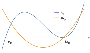
Figure 3: Simultaneous realizations of the criticality $\lambda_{\phi}\sim\beta_{\lambda_{\phi}}\sim 0$ at high-energy scale and the CW mechanism at low-energy scale.

$\ast$ Degeneracy with low-energy vacuum
An extremum at high-energy scales can degenerate with a low-energy extremum, i.e. $V|_{\phi=v_{\phi}}=V|_{\phi=\tilde{v}_{\phi}}$. Here, $\phi=v_{\phi}$ and $\phi=\tilde{v}_{\phi}$ are the low-energy and high-energy extrema, respectively. However, as long as $v_{\phi}\sim M\ll\tilde{v}_{\phi}$, $V|_{\phi=v_{\phi}}$ is negligibly small compared with the high-energy scales. Therefore the condition for the criticality is given by $V|_{\phi=\tilde{v}_{\phi}}=V^{\prime}|_{\phi=\tilde{v}_{\phi}}=0$. From Eq. (43) and Eq. (44), it is equivalent to

$$\lambda_{\phi}^{\rm eff}=\beta_{\lambda_{\phi}^{\rm eff}}=0~{},\quad\text{at $\phi=\tilde{v}_{\phi}$}~{}.$$ (45)

Note that this criticality is obtained by a one-parameter tuning of the coupling constants. Suppose that $\lambda_{\phi}^{\rm eff}>0$ and $\beta_{\lambda_{\phi}^{\rm eff}}<0$ at some large value of $\phi~{}(<\tilde{v}_{\phi})$. Then as $\phi$ is increased, $\lambda_{\phi}^{\rm eff}$ is expected to go to zero at a certain value of $\phi$, $\phi=\tilde{v}_{\phi}$. Eq. (45) requires that $\beta_{\lambda_{\phi}^{\rm eff}}$ goes to zero at the same time, which can be satisfied by adjusting one parameter. It is also worth pointing out that if we want absolute stability of a low-energy vacuum, $\lambda_{\phi}^{\rm eff}$ must be positive around $\phi\sim\tilde{v}_{\phi}$.

It is a rather complicated problem to obtain a higher critical point by combining this criticality with a low-energy criticality of the previous subsection. As we have seen there, at low-energy scale $\phi\sim M$, $\beta_{\lambda_{\phi}^{\rm eff}}$ needs to be positive in order to obtain a criticality. Thus, the beta function needs to flip its sign at some intermediate scale in order to archive simultaneous degeneracies among several low-energy extrema and a high-energy extremum. See Fig. 3 for example. Such a criticality, sometimes called the “flatland scenario” [28, 47, 48, 30], requires nontrivial RGEs and initial conditions of coupling constants for the sign of the beta function to flip. Note that in the SM with the observed coupling constants, the Higgs potential can satisfy Eq. (45) near the Planck scale, while it is difficult to realize the low-energy criticality as in the CW mechanism at the weak scale.

Let’s investigate the high-energy extrema of $V$ in a more concrete manner. First, we introduce an approximate expression of $\beta_{\lambda_{\phi}^{\rm eff}}$ around its zero point as

$$\beta_{\lambda_{\phi}^{\rm eff}}(\phi)\simeq b\ln\left(\phi/\mu_{\rm min}\right)~{},$$ (46)

by regarding $d\beta_{\lambda_{\phi}^{\rm eff}}/d\ln\phi:=b$ as a constant. In the following we assume $b>0$ for simplicity. Obviously, $\beta_{\lambda_{\phi}^{\rm eff}}$ becomes zero at $\phi=\mu_{\rm min}$. From this we obtain

$$\lambda_{\phi}^{\rm eff}(\phi)\simeq\lambda_{\rm min}+\frac{b}{2}\left[\ln\left(\phi/\mu_{\rm min}\right)\right]^{2}~{},$$ (47)

which takes the extremal value $\lambda_{\rm min}$ at $\phi=\mu_{\rm min}$. Then from Eq. (44), the extrema of $V$, $\phi=\tilde{v}_{\phi}$, are given by

$$\tilde{v}_{\phi}=\mu_{\rm min}\exp\left[\frac{1}{4}\left(-1\pm\sqrt{1-32\frac{\lambda_{\rm min}}{b}}\right)\right]~{}.$$ (48)

From Eqs. (43)(46)(48), it is clear that both the number of extrema and the sign of the minimum value of $V$ depend on the value of $r:=\lambda_{\rm min}/b~{}$: When $r<1/32$, $V$ has one minimum and one maximum at high-energy scales. In this region of $r$, the sign of the minimum value of $V$ is the same as that of $r$. When $r=1/32$, the minimum and maximum merge to form a saddle point, and they disappear when $r>1/32$. Obviously, the critical point we have considered above corresponds to $r=0$, i.e. $\lambda_{\rm min}=0$.

$\ast$ Saddle point criticality
Another possible criticality involving high-energy extrema is that they themselves degenerate. Because there is generically one minimum and one maximum, the only possibility for criticality is for them to degenerate and form a saddle point. The vanishing condition of the first derivative is the same as Eq. (44), while the condition for the second derivative is

$$V^{\prime\prime}|_{\phi=\tilde{v}_{\phi}}=0\quad\Leftrightarrow\quad\left[12\lambda_{\phi}^{\rm eff}+7\beta_{\lambda_{\phi}^{\rm eff}}+\frac{d\beta_{\lambda_{\phi}^{\rm eff}}}{d\ln\phi}\right]\bigg{|}_{\phi=\tilde{v}_{\phi}}=0~{}.$$ (49)

As long as $|d\beta_{\lambda_{\rm eff}}/d\ln\phi|\ll\lambda_{\phi}^{\rm eff},~{}|\beta_{\lambda_{\phi}^{\rm eff}}|$ and $\lambda_{\phi}^{\rm eff}>0$, this condition also requires $\beta_{\lambda_{\rm eff}}<0$. Indeed within the approximation Eq. (47), we have seen that we have a saddle point when $r=1/32$. In other words, $V(\phi)$ has a saddle point when

$$\lambda_{\rm min}=\frac{b}{32}~{},$$ (50)

and the location of the saddle point is $\tilde{v}_{\phi}=\mu_{\rm min}e^{-1/4}$.

$\bullet$ Implications for cosmology
The existence of high-energy vacuum or saddle point has a lot of implications for cosmology. One of the well-known examples is the critical (Higgs) inflation [7, 36, 8, 49, 40]. The inflation with non-minimal coupling $\xi\phi^{2}R/M_{\rm Pl}^{2}$ typically needs large $\xi\sim 10^{5}$ to explain the observed amplitude of the CMB fluctuations when $\lambda_{\phi}={\cal O}(0.1)$. However, the MPP naturally favors smallness of $\lambda_{\phi}\sim\beta_{\lambda_{\phi}}$ and this allows a successful inflation even when $\xi={\cal O}(10)$.

Moreover, the smallness of the quartic coupling is also important to discuss unitarity issue during the preheating stage after the inflation; As discussed in Refs. [50, 51, 52, 53, 54, 55], the background dynamics of the inflaton shows a spike-like behavior around its zero-crossings and can cause violent particle production of the Nambu-Goldstone modes of the inflaton or the longitudinal modes of the (weak) gauge bosons. In particular, the typical energy scale of those produced particles is ${\cal O}(\lambda_{\phi}^{1/2}M_{\rm Pl})$, which is much larger than the cutoff scale $\Lambda:=M_{\rm Pl}/\xi^{1/2}$ when $\xi\sim 10^{5}$.  Thus, the consistency (predictability) of the theory during the preheating stage is not clear. However, the situation changes quite a lot in the case of the critical (Higgs) inflation because the energy scale of produced particles is expected to be largely suppressed thanks to the smallness of $\lambda_{\phi}$. The resultant cosmological predictions such as the reheating temperature need more detailed study of particle production and we want to discuss this possibility in some future investigation.

Another interesting application of high-energy criticality is to generate a seed of primordial black holes (PBHs) [38]. When overdense regions in the Universe have sufficiently large density fluctuations $\delta\rho/\rho\gtrsim 0.4$, they can collapse into PBHs by overcoming the pressure of radiations. However, the observed fluctuations at large scales by the CMB is too small $\delta\rho/\rho\sim 10^{-5}$, and it is necessary to generate large fluctuations at small scales. Here, we can use the saddle point of the inflaton potential predicted by the MPP to obtain such large fluctuations. Naively, this can be seen by looking at the definition of the power spectrum of curvature perturbations in the slow-roll approximation

$${\cal P}_{R}=\frac{V(\phi)^{3}}{24\pi^{2}M_{\rm Pl}^{6}V^{\prime}(\phi)^{2}}~{},$$ (51)

which is proportional to $V^{\prime}(\phi)^{-2}$. However, detailed studies [57, 58, 59] have shown that this is too naive because (i) we can not rely on the usual slow-roll approximations at around the saddle point and (ii) the slow-roll conditions are violated right before the saddle point. Although the predictions of the large density fluctuations in the critical (Higgs) inflation model are still in questioned, utilizing saddle point as a seed of large density fluctuations is an interesting possibility and naturally favored by the MPP.

4 Summary and discussion

In this paper, we have studied the multi-critical points of the one-loop effective potential. In order to simplify our discussion, we have assumed that the other fields except $\phi$ are either massless or too heavy to contribute to the low energy effective potential of $\phi$. Then, we have located all the maximally critical points in the parameter space of $\lambda_{1}$, $m^{2}$, and $\lambda_{3}$. One of these critical points is just the conventional CW potential, but the MPP also predicts other multi-critical points that allow for a symmetry breaking, and they should be equally treated in this framework.

Phenomenological applications of these critical points are also interesting. They can have a lot of implications for cosmology since they can predict a (strong) first-order phase transition at the early universe. We want to report their consequences such as Gravitational Wave, electroweak baryogenesis, formation of primordial black holes etc. in the near future [60].

Appendix Appendix A Doubly critical points

The critical points (lines) which correspond to 2-parameter tunings are less attractive from the point of view of the MPP. Nevertheless, it would be meaningful to study them because a lot of extended models are (automatically) categorized into this case. By considering the redefinition $\phi\rightarrow-\phi$, the possible degeneracies are given by

$$123~{},\ 124~{},\ 125~{},\ 134~{},\ 135~{},\ 234~{},\$$ (52)

$$12-34~{},\ 12-35~{},\ 12-45 ~{},\ 13-24~{},\ 13-25~{},\ 14-23~{},\ 14-25~{},\ 15-23,\ 15-24~{}.$$ (53)

As in the case of the maximally critical points, it is easy to find that $14-23$ and $14-25$ are not realized by simply comparing the values of the extrema.

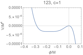
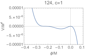
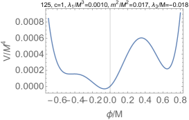
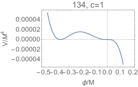
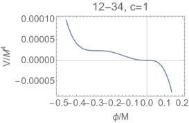
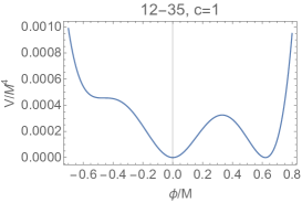
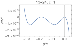
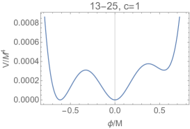
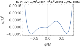
Figure 4: The effective potentials corresponding to the bicritical points.

Because these degeneracies are achieved by two-parameter tunings, each of them lies on a one-dimensional critical curves in the three dimensional parameter space of $\lambda_{1},m^{2},\lambda_{3}$. To specify such curves, we consider their intersections with the plane $\lambda_{1}=0$. In other word, we will simply set $\lambda_{1}=0$ except when necessary. It will be found that only $125$ and $15-23$ require $\lambda_{1}\neq 0$.

$\ast$ 123: This critical point is defined by $V^{\prime}|_{\phi=\phi_{S}}=V^{\prime\prime}|_{\phi=\phi_{S}}=V^{\prime\prime\prime}|_{\phi=\phi_{S}}=0$, and we can solve them analytically by using Eqs. (17)(18)(19). The results are

$$\phi_{S}=\mp Me^{-7/4}~{},\quad m^{2}=-\frac{c}{12}e^{-7/2}M^{2}~{},\quad\lambda_{3}=\mp\frac{2c}{3}e^{-7/4}M~{}.$$ (54)

$v_{\phi}$ and $m_{\phi}^{2}$ are numerically given by

$$v_{\phi}\simeq\pm 1.1M~{},\quad m_{\phi}^{2}=0.26cM^{2}~{}.$$ (55)

The resultant potential is shown in the upper-left panel in Fig. 4 where we focus on the field region $\phi<0$ so that the degeneracy of the extrema can be easily seen.

$\ast$ 124: This critical point is defined by $V|_{\phi=\phi_{S}}=V^{\prime}|_{\phi=\phi_{S}}=V^{\prime\prime}|_{\phi=\phi_{S}}=0$, and we can also solve them analytically by using Eqs. (17)(18). The results are

$$\phi_{S}=\mp Me^{-3/2}~{},\quad m^{2}=-\frac{c}{24}e^{-3}M^{2}~{},\quad\lambda_{3}=\mp\frac{c}{2}e^{-3/2}M~{}.$$ (56)

Then, $v_{\phi}$ and $m_{\phi}^{2}$ are numerically solved as

$$v_{\phi}\simeq\pm 1.1M~{},\quad m_{\phi}^{2}=0.26cM^{2}~{}.$$ (57)

The resultant potential is shown in the upper-middle panel in Fig. 4.

$\ast$ 125: As mentioned before, this critical point needs $\lambda_{1}\neq 0$ and we have one-parameter solution. In the upper-right panel in Fig. 4, we show one example of the potential whose parameters are numerically obtained as

$$c=1~{},\ \lambda_{1}=0.0010M^{3}~{},\ m^{2}=0.017M^{2}~{},\ \lambda_{3}=-0.018M~{}.$$ (58)

$\ast$ 134: This critical point can be obtained by putting $m^{2}=0$ and solving $V|_{\phi=v_{f}}=V^{\prime}|_{\phi=v_{f}}=0$ with respect to $\lambda_{3}$ and $v_{f}$. The solutions are

$$\lambda_{3}=\pm\frac{c}{4}Me^{-1}~{},\quad v_{f}=\pm Me^{-1}~{}.$$ (59)

Then, the true vacuum is determined by

$$\frac{\partial V}{\partial\phi}\bigg{|}_{\phi=v_{\phi}}=\frac{cv_{\phi}^{2}}{8}\left(v_{f}+\frac{2}{3}v_{\phi}\log\left(\frac{v_{\phi}^{2}}{M^{2}e^{-1/2}}\right)\right)=0~{}\quad\therefore\ 3v_{f}+4v_{\phi}\log\left(\frac{|v_{\phi}|}{Me^{-1/4}}\right)=0~{},$$ (60)

whose solution is

$$v_{\phi}=\mp M\exp\left[W\left(\frac{3|v_{f}|}{4Me^{-1/4}}\right)-\frac{1}{4}\right]=\mp M\exp\left[W\left(\frac{3}{4e^{3/4}}\right)-\frac{1}{4}\right]=\mp 1.0M~{},$$ (61)

where $W(z)$ is the Lambert $W$ function satisfying $z=e^{W}W$. The mass of $\phi$ is

$$m_{\phi}^{2}=\frac{\partial V^{2}}{\partial\phi^{2}}\bigg{|}_{\phi=v_{\phi}}=\frac{c}{6}\left(1+W\left(\frac{3}{4e^{3/4}}\right)\right)v_{\phi}^{2}=0.22cM^{2}~{}.$$ (62)

The resultant potential is shown in the middle-left panel in Fig. 4.

$\ast$ 135 (15-24): This critical point is the same as $135-24$. Thus, the parameters are given by Eq. (34).

$\ast$ 234: This critical point is also the same as $234-15$. Thus, the potential and the parameters are given by Eqs. (35)(36).

$\ast$ 12-34: By the saddle point conditions $V^{\prime}|_{\phi=\phi_{S}}=V^{\prime\prime}|_{\phi=\phi_{S}}=0$, $m^{2}$ and $\lambda_{3}$ can be solved as functions of $\phi_{S}$:

$$m^{2}=\frac{c\phi_{S}^{2}}{12}\left(\frac{5}{2}+\log\left(\frac{\phi_{S}^{2}}{M^{2}}\right)\right)~{},\quad\lambda_{3}=-\frac{c\phi_{S}}{3}\left(\frac{3}{2}+\log\left(\frac{\phi_{S}^{2}}{M^{2}}\right)\right)~{}.$$ (63)

The critical point $12-34$ is given by the solution of $m^{2}=0$;

$$\lambda_{3}=\pm\frac{c}{3}Me^{-5/4}~{},\quad\phi_{S}=\pm Me^{-5/4}~{},$$ (64)

and the corresponding true vacuum is determined by

$$\frac{\partial V}{\partial\phi}\bigg{|}_{\phi=v_{s}}=\frac{c}{6}v_{\phi}^{2}\left(\phi_{S}+\frac{v_{\phi}}{2}\log\left(\frac{v_{\phi}^{2}}{M^{2}e^{-1/2}}\right)\right)=0~{},$$ (65)

$$\therefore\ v_{\phi} =\mp M\exp\left[W\left(\frac{|\phi_{S}|}{Me^{-1/4}}\right)-\frac{1}{4}\right]=\mp M\exp\left[W\left(e^{-1}\right)-\frac{1}{4}\right]=\mp 1.0M$$ (66)

The mass of $\phi$ is given by

$$m_{\phi}^{2}=\frac{\partial V^{2}}{\partial\phi^{2}}\bigg{|}_{\phi=v_{\phi}}=\frac{c}{6}\left(1+W(e^{-1})\right)v_{\phi}^{2}=0.23cM^{2}~{}.$$ (67)

The resultant potential is shown in the center panel in Fig. 4.

$\ast$ 12-35: This critical point can be obtained by putting Eq. (63) into the potential and solving $V|_{\phi=v_{\phi}}=V^{\prime}|_{\phi=v_{\phi}}=0$ as functions of $v_{\phi}$ and $\phi_{S}$. The numerical results are

$$v_{\phi}\simeq\pm 0.62M~{},\quad\phi_{S}\simeq\mp 0.46M~{},\quad m^{2}\simeq 0.017cM^{2}~{},\quad\lambda_{3}\simeq\mp 0.0075cM~{}.$$ (68)

Then, the mass of $\phi$ is calculated as

$$m_{\phi}^{2}=\frac{\partial^{2}V}{\partial\phi^{2}}\bigg{|}_{\phi=v_{\phi}}\simeq\begin{cases}0.017cM^{2}&\text{for $v_{\phi}=0$}\\ 0.033cM^{2}&\text{for $|v_{\phi}|=0.62M$}\end{cases}~{}.$$ (69)

The resultant potential is shown in the middle-right panel in Fig. 4.

$\ast$ 12-45: This critical point is the same as $1245$. Thus, the parameters are given by Eqs. (28)(29).

$\ast$ 13-24: The $24$ degeneracy is defined by $V|_{\phi=\phi_{2}}=V^{\prime}|_{\phi=\phi_{2}}=0$ and this can be solved as

$$m^{2}=\frac{c}{24}\phi_{2}^{2}\left(2+1\log\left(\frac{\phi_{2}^{2}}{M^{2}}\right)\right)~{},\quad\lambda_{3}=-\frac{c}{4}\phi_{2}\left(1+\log\left(\frac{\phi_{2}^{2}}{M^{2}}\right)\right)~{},$$ (70)

Then, the degeneracy between $1$ and $3$ can be numerically solved by putting Eq. (70) into $V(\phi)$ and changing $\phi_{2}$. The results are

$$v_{\phi}\simeq\pm 1.1M~{},\quad m^{2}\simeq-0.0020cM^{2}~{},\quad\lambda_{3}\simeq\mp 0.11cM~{},\quad m_{\phi}^{2}\simeq 0.25cM^{2}~{}.$$ (71)

The resultant potential is shown in the lower-left panel in Fig. 4.

$\ast$ 13-25: The $13$ degeneracy is the same as Eq. (70) with the replacement $\phi_{2}\rightarrow\phi_{1}$. Then, the degeneracy $25$ can be numerically found by putting them into $V(\phi)$ and changing $\phi_{1}$. The results are

$$m^{2}\simeq 0.016cM^{2}~{},\quad\lambda_{3}\simeq\mp 0.0046cM~{},\quad(v_{\phi},m_{\phi}^{2})\simeq\begin{cases}(\pm 0.62M,0.032cM^{2})&{\rm for}\ 1\\ (0,0.016cM^{2})&{\rm for}\ 3\end{cases}~{}.$$ (72)

The resultant potential is shown in the lower-middle panel in Fig. 4.

$\ast$ 15-23: As mentioned before, this critical point needs $\lambda_{1}\neq 0$ and we have one-parameter solution. In the lower-right panel in Fig. 4, we show one example of the potential whose parameters are numerically obtained as

$$c=1~{},\ \lambda_{1}=0.0010M^{3}~{},\ m^{2}=0.013M^{2}~{},\ \lambda_{3}=-0.014M~{}.$$ (73)

In Table. 2, we summarize all the doubly critical points corresponding to 2-parameter tuning.

	$\mathbb{Z}_{2}$	$|v_{\phi}|$	$m_{\phi}^{2}$	$\lambda_{1}$
123	Broken	$1.1M$	$0.26cM^{2}$	0
124	Broken	$1.1M$	$0.26cM^{2}$	0
125	Broken	-	-	$\neq 0$
134	Broken	$Me^{-1/4}\exp\left\{W(3e^{-3/4}/4))\right\}$	$cv_{\phi}^{2}(1+W(3e^{-3/4}/4))/6$	0
135 (15-24)	Exact	$Me^{-1/2}$	$cM^{2}e^{-1}/12$	0
234	Exact	$Me^{-1/4}$	$cM^{2}e^{-1/2}/6$	0
12-34	Broken	$Me^{-1/4}\exp\left\{W(e^{-1}))\right\}$	$cv_{\phi}^{2}(1+W(e^{-1}))/6$	0
12-35	Broken	$0$ or $0.62M$	$0.017cM^{2}$ or $0.033cM^{2}$	0
12-45	Exact	$0$	$cM^{2}e^{-3/2}/12$	0
13-24	Broken	$1.1M$	$0.25cM^{2}$	0
13-25	Broken	$0$ or $0.62M$	$0.016cM^{2}$ or $0.032cM^{2}$	0
15-23	Broken	-	-	$\neq 0$

Table 2: All the critical points of the one-loop effective potential Eq. (16) corresponding to 2-parameter tuning.

References

- [1] G. Degrassi, S. Di Vita, J. Elias-Miro, J. R. Espinosa, G. F. Giudice, G. Isidori, and A. Strumia, “Higgs mass and vacuum stability in the Standard Model at NNLO,” JHEP 08 (2012) 098, arXiv:1205.6497 [hep-ph].
- [2] D. Buttazzo, G. Degrassi, P. P. Giardino, G. F. Giudice, F. Sala, A. Salvio, and A. Strumia, “Investigating the near-criticality of the Higgs boson,” JHEP 12 (2013) 089, arXiv:1307.3536 [hep-ph].
- [3] A. Bednyakov, B. Kniehl, A. Pikelner, and O. Veretin, “Stability of the Electroweak Vacuum: Gauge Independence and Advanced Precision,” Phys. Rev. Lett. 115 no. 20, (2015) 201802, arXiv:1507.08833 [hep-ph].
- [4] Y. Hamada, H. Kawai, and K.-y. Oda, “Bare Higgs mass at Planck scale,” Phys. Rev. D 87 no. 5, (2013) 053009, arXiv:1210.2538 [hep-ph]. [Erratum: Phys.Rev.D 89, 059901 (2014)].
- [5] M. Holthausen, K. S. Lim, and M. Lindner, “Planck scale Boundary Conditions and the Higgs Mass,” JHEP 02 (2012) 037, arXiv:1112.2415 [hep-ph].
- [6] F. Bezrukov, M. Y. Kalmykov, B. A. Kniehl, and M. Shaposhnikov, “Higgs Boson Mass and New Physics,” JHEP 10 (2012) 140, arXiv:1205.2893 [hep-ph].
- [7] Y. Hamada, H. Kawai, K.-y. Oda, and S. C. Park, “Higgs inflation from Standard Model criticality,” Phys. Rev. D 91 (2015) 053008, arXiv:1408.4864 [hep-ph].
- [8] Y. Hamada, H. Kawai, and K.-y. Oda, “Predictions on mass of Higgs portal scalar dark matter from Higgs inflation and flat potential,” JHEP 07 (2014) 026, arXiv:1404.6141 [hep-ph].
- [9] P. Z. et al. (Particle Data Group), “The review of particle physics,” Prog. Theor. Exp. Phys. 2020 (2020) 083C01.
- [10] C. Froggatt and H. B. Nielsen, “Standard model criticality prediction: Top mass 173 +- 5-GeV and Higgs mass 135 +- 9-GeV,” Phys. Lett. B 368 (1996) 96–102, arXiv:hep-ph/9511371.
- [11] C. Froggatt, H. B. Nielsen, and Y. Takanishi, “Standard model Higgs boson mass from borderline metastability of the vacuum,” Phys.Rev. D64 (2001) 113014, arXiv:hep-ph/0104161 [hep-ph].
- [12] H. B. Nielsen, “PREdicted the Higgs Mass,” Bled Workshops Phys. 13 no. 2, (2012) 94–126, arXiv:1212.5716 [hep-ph].
- [13] H. Kawai and T. Okada, “Asymptotically Vanishing Cosmological Constant in the Multiverse,” Int. J. Mod. Phys. A 26 (2011) 3107–3120, arXiv:1104.1764 [hep-th].
- [14] H. Kawai and T. Okada, “Solving the Naturalness Problem by Baby Universes in the Lorentzian Multiverse,” Prog. Theor. Phys. 127 (2012) 689–721, arXiv:1110.2303 [hep-th].
- [15] H. Kawai, “Low energy effective action of quantum gravity and the naturalness problem,” Int. J. Mod. Phys. A 28 (2013) 1340001.
- [16] Y. Hamada, H. Kawai, and K. Kawana, “Evidence of the Big Fix,” Int. J. Mod. Phys. A 29 (2014) 1450099, arXiv:1405.1310 [hep-ph].
- [17] Y. Hamada, H. Kawai, and K. Kawana, “Weak Scale From the Maximum Entropy Principle,” PTEP 2015 (2015) 033B06, arXiv:1409.6508 [hep-ph].
- [18] Y. Hamada, H. Kawai, and K. Kawana, “Natural solution to the naturalness problem: The universe does fine-tuning,” PTEP 2015 no. 12, (2015) 123B03, arXiv:1509.05955 [hep-th].
- [19] Y. Hamada, H. Kawai, and K.-y. Oda, “Eternal Higgs inflation and the cosmological constant problem,” Phys. Rev. D 92 (2015) 045009, arXiv:1501.04455 [hep-ph].
- [20] K. Kannike, N. Koivunen, and M. Raidal, “Principle of Multiple Point Criticality in Multi-Scalar Dark Matter Models,” arXiv:2010.09718 [hep-ph].
- [21] K. A. Meissner and H. Nicolai, “Conformal Symmetry and the Standard Model,” Phys.Lett. B648 (2007) 312–317, arXiv:hep-th/0612165 [hep-th].
- [22] R. Foot, A. Kobakhidze, K. L. McDonald, and R. R. Volkas, “A Solution to the hierarchy problem from an almost decoupled hidden sector within a classically scale invariant theory,” Phys.Rev. D77 (2008) 035006, arXiv:0709.2750 [hep-ph].
- [23] S. Iso, N. Okada, and Y. Orikasa, “Classically conformal extended Standard Model,” Phys.Lett. B676 (2009) 81–87, arXiv:0902.4050 [hep-ph].
- [24] S. Iso, N. Okada, and Y. Orikasa, “The minimal model naturally realized at TeV scale,” Phys.Rev. D80 (2009) 115007, arXiv:0909.0128 [hep-ph].
- [25] T. Hur and P. Ko, “Scale invariant extension of the standard model with strongly interacting hidden sector,” Phys.Rev.Lett. 106 (2011) 141802, arXiv:1103.2571 [hep-ph].
- [26] S. Iso and Y. Orikasa, “TeV Scale B-L model with a flat Higgs potential at the Planck scale - in view of the hierarchy problem -,” PTEP 2013 (2013) 023B08, arXiv:1210.2848 [hep-ph].
- [27] C. Englert, J. Jaeckel, V. Khoze, and M. Spannowsky, “Emergence of the Electroweak Scale through the Higgs Portal,” JHEP 04 (2013) 060, arXiv:1301.4224 [hep-ph].
- [28] M. Hashimoto, S. Iso, and Y. Orikasa, “Radiative symmetry breaking at the Fermi scale and flat potential at the Planck scale,” Phys. Rev. D 89 no. 1, (2014) 016019, arXiv:1310.4304 [hep-ph].
- [29] M. Holthausen, J. Kubo, K. S. Lim, and M. Lindner, “Electroweak and Conformal Symmetry Breaking by a Strongly Coupled Hidden Sector,” JHEP 12 (2013) 076, arXiv:1310.4423 [hep-ph].
- [30] M. Hashimoto, S. Iso, and Y. Orikasa, “Radiative symmetry breaking from flat potential in various U(1)’ models,” Phys. Rev. D 89 no. 5, (2014) 056010, arXiv:1401.5944 [hep-ph].
- [31] J. Kubo, K. S. Lim, and M. Lindner, “Electroweak Symmetry Breaking via QCD,” Phys.Rev.Lett. 113 (2014) 091604, arXiv:1403.4262 [hep-ph].
- [32] J. Kubo and M. Yamada, “Genesis of electroweak and dark matter scales from a bilinear scalar condensate,” Phys. Rev. D 93 no. 7, (2016) 075016, arXiv:1505.05971 [hep-ph].
- [33] K. Kawana, “Criticality and inflation of the gauged B – L model,” PTEP 2015 (2015) 073B04, arXiv:1501.04482 [hep-ph].
- [34] D.-W. Jung, J. Lee, and S.-H. Nam, “Scalar dark matter in the conformally invariant extension of the standard model,” Phys. Lett. B 797 (2019) 134823, arXiv:1904.10209 [hep-ph].
- [35] S. Jung and K. Kawana, “Low-energy probes of small CMB amplitude in models of radiative Higgs mechanism,” arXiv:2105.01217 [hep-ph].
- [36] F. Bezrukov and M. Shaposhnikov, “Higgs inflation at the critical point,” Phys. Lett. B 734 (2014) 249–254, arXiv:1403.6078 [hep-ph].
- [37] G. Ballesteros and C. Tamarit, “Radiative plateau inflation,” JHEP 02 (2016) 153, arXiv:1510.05669 [hep-ph].
- [38] J. M. Ezquiaga, J. Garcia-Bellido, and E. Ruiz Morales, “Primordial Black Hole production in Critical Higgs Inflation,” Phys. Lett. B 776 (2018) 345–349, arXiv:1705.04861 [astro-ph.CO].
- [39] S. M. Lee, K.-y. Oda, and S. C. Park, “Spontaneous Leptogenesis in Higgs Inflation,” arXiv:2010.07563 [hep-ph].
- [40] Y. Hamada, H. Kawai, K. Kawana, K.-y. Oda, and K. Yagyu, “Minimal scenario of Criticality for Electroweak scale, Neutrino Masses, Dark Matter, and Inflation,” arXiv:2102.04617 [hep-ph].
- [41] D. Y. Cheong, S. M. Lee, and S. C. Park, “Progress in Higgs inflation,” J. Korean Phys. Soc. 78 no. 10, (2021) 897–906, arXiv:2103.00177 [hep-ph].
- [42] M. Bando, T. Kugo, N. Maekawa, and H. Nakano, “Improving the effective potential: Multimass scale case,” Prog. Theor. Phys. 90 (1993) 405–418, arXiv:hep-ph/9210229.
- [43] S. Iso and K. Kawana, “RG-improvement of the effective action with multiple mass scales,” JHEP 03 (2018) 165, arXiv:1801.01731 [hep-ph].
- [44] S. R. Coleman and E. J. Weinberg, “Radiative Corrections as the Origin of Spontaneous Symmetry Breaking,” Phys. Rev. D 7 (1973) 1888–1910.
- [45] J. Haruna and H. Kawai, “Weak scale from Planck scale: Mass scale generation in a classically conformal two-scalar system,” PTEP 2020 no. 3, (2020) 033B01, arXiv:1905.05656 [hep-th].
- [46] Y. Hamada, H. Kawai, K.-y. Oda, and K. Yagyu, “Dark matter in minimal dimensional transmutation with multipoint criticality principle,” arXiv:2008.08700 [hep-ph].
- [47] E. J. Chun, S. Jung, and H. M. Lee, “Radiative generation of the Higgs potential,” Phys. Lett. B 725 (2013) 158–163, arXiv:1304.5815 [hep-ph]. [Erratum: Phys.Lett.B 730, 357–359 (2014)].
- [48] M. Ibe, S. Matsumoto, and T. T. Yanagida, “Flat Higgs Potential from Planck Scale Supersymmetry Breaking,” Phys. Lett. B 732 (2014) 214–217, arXiv:1312.7108 [hep-ph].
- [49] Y. Hamada, H. Kawai, Y. Nakanishi, and K.-y. Oda, “Cosmological implications of Standard Model criticality and Higgs inflation,” Nucl. Phys. B 953 (2020) 114946, arXiv:1709.09350 [hep-ph].
- [50] Y. Ema, R. Jinno, K. Mukaida, and K. Nakayama, “Violent Preheating in Inflation with Nonminimal Coupling,” JCAP 02 (2017) 045, arXiv:1609.05209 [hep-ph].
- [51] M. P. DeCross, D. I. Kaiser, A. Prabhu, C. Prescod-Weinstein, and E. I. Sfakianakis, “Preheating after Multifield Inflation with Nonminimal Couplings, I: Covariant Formalism and Attractor Behavior,” Phys. Rev. D 97 no. 2, (2018) 023526, arXiv:1510.08553 [astro-ph.CO].
- [52] M. P. DeCross, D. I. Kaiser, A. Prabhu, C. Prescod-Weinstein, and E. I. Sfakianakis, “Preheating after multifield inflation with nonminimal couplings, II: Resonance Structure,” Phys. Rev. D 97 no. 2, (2018) 023527, arXiv:1610.08868 [astro-ph.CO].
- [53] M. P. DeCross, D. I. Kaiser, A. Prabhu, C. Prescod-Weinstein, and E. I. Sfakianakis, “Preheating after multifield inflation with nonminimal couplings, III: Dynamical spacetime results,” Phys. Rev. D 97 no. 2, (2018) 023528, arXiv:1610.08916 [astro-ph.CO].
- [54] E. I. Sfakianakis and J. van de Vis, “Preheating after Higgs Inflation: Self-Resonance and Gauge boson production,” Phys. Rev. D 99 no. 8, (2019) 083519, arXiv:1810.01304 [hep-ph].
- [55] Y. Ema, R. Jinno, K. Nakayama, and J. van de Vis, “Preheating from target space curvature and unitarity violation: Analysis in field space,” Phys. Rev. D 103 no. 10, (2021) 103536, arXiv:2102.12501 [hep-ph].
- [56] Y. Hamada, K. Kawana, and A. Scherlis, “On Preheating in Higgs Inflation,” JCAP 03 (2021) 062, arXiv:2007.04701 [hep-ph].
- [57] C. Germani and T. Prokopec, “On primordial black holes from an inflection point,” Phys. Dark Univ. 18 (2017) 6–10, arXiv:1706.04226 [astro-ph.CO].
- [58] M. Drees and Y. Xu, “Overshooting, Critical Higgs Inflation and Second Order Gravitational Wave Signatures,” Eur. Phys. J. C 81 no. 2, (2021) 182, arXiv:1905.13581 [hep-ph].
- [59] J. Liu, Z.-K. Guo, and R.-G. Cai, “Analytical approximation of the scalar spectrum in the ultraslow-roll inflationary models,” Phys. Rev. D 101 no. 8, (2020) 083535, arXiv:2003.02075 [astro-ph.CO].
- [60] Y. Hamada, H. Kawai, K. Kawana, K.-y. Oda, and K. Yagyu, “To appear,” arXiv:XXXX [hep-ph].