Cell-free Massive MIMO with Short Packets

Abstract

In this paper, we adapt to cell-free Massive MIMO (multiple-input multiple-output) the finite-blocklength framework introduced by Östman et al. (2020) for the characterization of the packet error probability achievable with Massive MIMO, in the ultra-reliable low-latency communications (URLLC) regime. The framework considered in this paper encompasses a cell-free architecture with imperfect channel-state information, and arbitrary linear signal processing performed at a central-processing unit connected to the access points via fronthaul links. By means of numerical simulations, we show that, to achieve the high reliability requirements in URLLC, MMSE signal processing must be used. Comparisons are also made with both small-cell and Massive MIMO cellular networks. Both require a much larger number of antennas to achieve comparable performance to cell-free Massive MIMO.

I Introduction

Massive multiple-input multiple-output (MIMO) is a key technology in 5G, owing to its ability to substantially increase the spectral efficiency of cellular networks [1]. An important challenge in Massive MIMO is the large pathloss variations and inter-cell interference, in particular for the cell-edge user equipments (UEs) [2]. An alternative network structure, known as cell-free Massive MIMO, was recently proposed to overcome this issue [3, 4]. In this type of network, all the UEs in a large coverage area may be jointly served by multiple distributed access points (APs). The fronthaul connections between the APs and the central processing unit (CPU), enable the division of the processing tasks for coherently serving all the active UEs.

The aim of this paper is to investigate the design of cell-free Massive MIMO architectures to support ultra-reliable low-latency communications (URLLC)—a novel use case in next-generation wireless systems (5G and beyond) aimed at providing connectivity to real-time mission-critical applications, such as remote control of automated factories [5]. The low latency required in such applications and the typically small payload contained by the transmitted data packets, make the use of nonasymptotic (i.e., finite-blocklength) information theoretic tools fundamental for the design of such systems [6].

State of the Art

In most of the recent literature where the advantages of cell-free Massive MIMO over traditional architectures are illustrated, ergodic capacity is used as performance metric (see, e.g., [7] and references therein). Unfortunately, this metric is asymptotic in the blocklength and, hence, not adequate for scenarios in which the packet length is short due to latency constraints. One recent exception is [8], where a conjugate beamforming scheme for cell-free Massive MIMO architectures is developed on the basis of the so-called normal approximation [9]. Unfortunately, this approximation, although capturing finite-blocklength effects, tends to loose accuracy at the low error probabilities that are of interest in URLLC [10]. Furthermore, the analysis in [8] is conducted under the assumption of perfect channel state information (CSI). Hence, it neglects the overhead due to pilot transmission, which is often significant in the short-blocklength regime [11].

Contributions

We illustrate how to use the so-called random-coding union bound with parameter $s$ (RCUs) from finite-blocklength length information theory [12], to derive both a firm upper bound, and an easy-to compute approximation, based on the saddlepoint method [13, Sec. XVI], on the uplink (UL) and downlink (DL) error probabilities achievable in a cell-free Massive MIMO system deployed to support URLLC. To do so, we extend to cell-free Massive-MIMO the finite-blocklength framework derived in [10] for cellular Massive-MIMO networks. Numerical simulations are used to show that, in a practically relevant automated-factory deployment scenario, cell-free Massive MIMO with fully centralized processing outperforms cellular Massive MIMO in terms of the fraction of the coverage area in which URLLC services can be provided.

Notation

Lower-case bold letters are used for vectors and upper-case bold letters are used for matrices. The circularly-symmetric Gaussian distribution is denoted by $\mathcal{CN}(0,\sigma^{2})$, where $\sigma^{2}$ denotes the variance. We use $\operatorname{\mathbb{E}}\mathopen{}\left[\cdot\right]$ to indicate the expectation operator, and $\mathbb{P}\mathopen{}\left[{\cdot}\right]$ for the probability of a set. The natural logarithm is denoted by $\log(\cdot)$.

II A Finite-Blocklength Upper-Bound on the Error Probability

A finite-blocklength information-theoretic upper bound on the error probability achievable in a cell-free Massive MIMO architecture needs to capture the following elements:

• it must allow for linear processing to separate the signals generated by/intended to the different UEs;

• it must allow for pilot-based CSI acquisition and apply to the scenario where decoding is performed by assuming that the acquired CSI is exact;

• it must apply to a scenario in which the additive noise term includes not only thermal noise, but also channel estimation error and residual multiuser interference after linear processing.

A bound satisfying this requirement is the so-called RCUs given in [12]. To introduce this bound, let us consider the following scalar input-output relation:

$$v[k]=gq[k]+z[k],\quad k=1,\dots,n.$$ (1)

Here, $q[k]$ denotes the $k$th entry of the length-$n$ codeword transmitted by a given user, $v[k]$ is the corresponding received signal after linear processing, $g$ denotes the effective channel after linear processing, which we assume to stay constant over the duration of the packet, and $z[k]$ is the additive noise signal, which also includes the residual multiuser interference after linear processing.

To derive the bound, we shall assume that the receiver does not know $g$ but has access to an estimate $\widehat{g}$ that is treated as perfect. This estimate may be obtained via pilot transmission, or may simply be based on the knowledge of first-order statistics of $g$. The first situation is relevant in the UL of Massive MIMO, whereas the second situation typically occurs in the DL (see, e.g., [14]).

To determine the transmitted codeword, the decoder performs scaled nearest-neighbor (SNN) decoding, i.e., it seeks the codeword that, after being scaled by the estimated channel gain $\hat{g}$, is closest to the received vector. Mathematically, the decoder solves the following optimization problem:

$$\widehat{}\mathbf{q}=\operatorname*{arg\;min}_{\widetilde{}\mathbf{q}\in\mathcal{C}}\lVert\mathbf{v}-\widehat{g}\widetilde{}\mathbf{q}\rVert^{2}.$$ (2)

Here, $\mathbf{v}=[v[1],\dots,v[n]]^{\mbox{\tiny$\mathrm{T}$}}$, the vector $\widehat{}\mathbf{q}$ stands for the codeword chosen by the decoder, and $\mathcal{C}$ denotes the set of length-$n$ codewords.

The RCUs provides a random coding bound on the error probability $\epsilon=\mathbb{P}\mathopen{}\left[{\widehat{}\mathbf{q}\neq\mathbf{q}}\right]$ achieved when the decoder operates according to the rule (2). The following theorem provides such a bound for the so-called Gaussian random ensemble.

Theorem 1 (​​[10, Th. 1])

Assume that $g\in\mathbb{C}$ and $\widehat{g}\in\mathbb{C}$ in (1) are random variables drawn according to an arbitrary joint distribution. There exists a coding scheme with $m=2^{b}$ codewords of length $n$ operating according to the mismatched SNN decoding rule (2), whose error probability $\epsilon$ is upper-bounded by

$$\epsilon = \mathbb{P}\mathopen{}\left[{\widehat{}\mathbf{q}\neq\mathbf{q}}\right]$$ (3)

$$\leq \operatorname{\mathbb{E}}_{g,\widehat{g}}\mathopen{}\left[\mathbb{P}\mathopen{}\left[{\sum_{k=1}^{n}{\imath_{s}(q[k],v[k])}\leq\log\frac{m-1}{u}\bigg{|}g,\widehat{g}}\right]\right]$$

for all $s>0$. Here, $u$ is a random variable that is uniformly distributed over the interval $[0,1]$ and $\imath_{s}(q[k],v[k])$ is the so-called generalized information density, given by

$$\imath_{s}(q[k],v[k])=-s\left|{v[k]-\widehat{g}q[k]}\right|^{2}\\ +\frac{s\lvert v[k]\rvert^{2}}{1+s\rho\lvert\widehat{g}\rvert^{2}}+\log\mathopen{}\left({1+s\rho\lvert\widehat{g}\rvert^{2}}\right).$$ (4)

Finally, the average in (3) is taken over the joint distribution of $g$ and $\widehat{g}$.

Proof:

See [10, App. A]. ∎

We refer the interested reader to [10] for more details about this bound, including its relation to the so-called generalized mutual information. Note that the bound is valid for all values of $s>0$ and can be tightened by performing an optimization over this parameter.

Unfortunately, the bound (3) is difficult to evaluate numerically. Indeed, the probability inside the expectation in (3) is not known in closed form, and evaluating it accurately for the error-probabilities of interest in URLLC is time consuming. One common approach to simplify its evaluation is to invoke the Berry-Esseen central limit theorem [13, Ch. XVI.5] and replace the probability in (3) with a closed-form approximation that involves the Gaussian $Q(\cdot)$ function and the first two moments of the generalized information density, which are known in closed form. The resulting approximation, which is usually referred to as the normal approximation, has been recently used in [8] within cell-free Massive MIMO analyses. Unfortunately, as shown in [10, Fig. 1], this approximation is accurate only when the rate $R=(\log m)/n$ is close to the expected value of the generalized information density; this is typically not the case for the low error-probabilities of interest in URLLC.

An alternative approximation, which turns out to be accurate for a much larger range of error-probability values, including the ones of interest in URLLC, can be obtained using the so-called saddlepoint method [13, Ch. XVI]. The resulting approximation is also in closed form for the setup considered in the present paper. As a consequence, the saddlepoint approximation has essentially the same computational complexity as the normal approximation (although its overall expression, given in [10, Th. 2], is arguably more involved). The saddlepoint approximation depends on the cumulant generating function of the generalized information density and on its first and second derivatives, evaluated at a point that depends on the chosen rate $R$. In contrast, the normal approximation depends on the mean and the variance of the generalized information density, i.e., on the value of the first and second-order derivatives of the cumulant generating function computed at the fixed value $0$.

III Cell-free Massive MIMO Network

We consider a fully centralized network with $L$ APs, each equipped with $M$ antennas, which are geographically distributed over the coverage area. The APs serve jointly $K$ single-antenna UEs, and are connected via fronthaul links to a CPU, which facilitates the AP coordination. The standard time-division duplexing protocol of cellular Massive MIMO is used, where the $n$ available channel uses are used for three purposes: $n_{\text{{}p}}$ symbols for UL pilots; $n_{\rm ul}$ symbols for UL data; and $n_{\rm dl}$ symbols for DL data. The signals received by each AP are sent to the CPU over the frounthaul links. Then, the CPU performs both channel estimation and data detection.

The channel between AP $l$ and UE $i$ is denoted by ${\bf h}_{il}\in\mathbb{C}^{M}$. We use a correlated Rayleigh fading model where ${\bf h}_{il}\sim\mathcal{CN}({\bf 0}_{M},{\bf R}_{il})$ remains constant for the duration of a codeword transmission. The normalized trace $\beta_{il}=\mathrm{tr}({\bf{R}}_{il})/M$ determines the average large-scale fading between AP $l$ and UE $i$, while the eigenstructure of ${\bf{R}}_{il}$ describes its spatial channel correlation [14, Sec. 2.2]. The collective channel vector ${\bf h}_{i}=[{\bf h}_{i1}^{\mbox{\tiny$\mathrm{T}$}}\ldots{\bf h}_{iL}^{\mbox{\tiny$\mathrm{T}$}}]^{\mbox{\tiny$\mathrm{T}$}}\in\mathbb{C}^{ML}$ follows a $\mathcal{CN}({\bf 0}_{ML},{\bf{R}}_{i})$ distribution, where ${\bf{R}}_{i}=\mathrm{diag}({\bf{R}}_{i1},\ldots,{\bf{R}}_{iL})$.

III-A Pilot Transmission and Channel Estimation

The UL pilot signature of UE $i$ is denoted by $\bm{\phi}_{i}\in\mathbb{C}^{n_{\text{{}p}}}$ and satisfies $\|\bm{\phi}_{i}\|^{2}=n_{\text{{}p}}$. The elements of $\bm{\phi}_{i}$ are scaled by the square-root of the pilot power $\sqrt{\rho^{\mathrm{ul}}}$ and transmitted over $n_{\text{{}p}}$ channel uses. This yields the received signal

$${\bf Y}_{l}^{\mathrm{pilot}}=\sqrt{\rho^{\mathrm{ul}}}\sum_{i=1}^{K}\mathbf{h}_{il}\bm{\phi}_{i}^{\mbox{\tiny$\mathrm{H}$}}+{\bf Z}_{l}^{\mathrm{pilot}}$$ (5)

where ${\bf Z}_{l}^{\mathrm{pilot}}\in\mathbb{C}^{M\times n_{\text{{}p}}}$ is noise with i.i.d. elements distributed as $\mathcal{CN}(0,\sigma_{\rm{ul}}^{2})$. Assuming that the covariance matrices $\{\mathbf{R}_{il}\}$ are known at the CPU, the minimum mean-square error (MMSE) estimate of $\mathbf{h}_{il}$ is [14, Sec. 3.2]

$$\widehat{}\mathbf{h}_{il}=\sqrt{\rho^{\mathrm{ul}}n_{\text{{}p}}}{\bf R}_{il}{\bf Q}_{il}^{-1}\left({\bf Y}_{l}^{\mathrm{pilot}}\bm{\phi}_{i}\right)$$ (6)

with ${\bf Q}_{il}=\rho^{\mathrm{ul}}\sum_{i=1}^{K}{\bf R}_{il}+\sigma_{\mathrm{ul}}^{2}{\bf I}_{M}.$ The MMSE estimate $\widehat{}\mathbf{h}_{il}$ and the estimation error $\widetilde{}\mathbf{h}_{il}=\mathbf{h}_{il}-\widehat{}\mathbf{h}_{il}$ are independent random vectors, distributed as $\widehat{}\mathbf{h}_{il}\sim\mathcal{CN}({\bf 0},{\bf\Phi}_{il})$ and $\widetilde{\mathbf{h}}_{il}\sim\mathcal{CN}({\bf 0},{\bf R}_{il}-{\bf\Phi}_{il})$, respectively, with ${\bf\Phi}_{il}={\rho^{\mathrm{ul}}n_{\text{{}p}}}{\bf R}_{il}{\bf Q}_{il}^{-1}{\bf R}_{il}$. To perform coherent processing of the signals at multiple APs, it is necessary to have knowledge of the collective channel ${\bf h}_{i}$, whose estimate is obtained as $\widehat{\bf h}_{i}=[\widehat{\bf h}_{i1}^{\mbox{\tiny$\mathrm{T}$}}\ldots\widehat{\bf h}_{iL}^{\mbox{\tiny$\mathrm{T}$}}]^{\mbox{\tiny$\mathrm{T}$}}$.

III-B Uplink Data Transmission

We denote by $x_{i}^{\rm ul}[k]$ the signal transmitted by UE $i$ over channel use $k$. In the UL of a fully centralized operation, each AP $l$ acts only as a remote-radio head, i.e., as a relay that forwards its received baseband signal ${\bf r}_{l}^{\rm{ul}}[k]$ to the CPU, which performs detection after linear processing. Specifically, for $k=1,\ldots,n_{\rm ul}$, the CPU computes

$$y_{i}^{\rm{ul}}[k]=\sum\limits_{l=1}^{L}{\bf u}_{il}^{\mbox{\tiny$\mathrm{H}$}}{\bf r}_{l}^{\rm{ul}}[k]={\bf u}_{i}^{\mbox{\tiny$\mathrm{H}$}}{\bf r}^{\rm{ul}}[k]$$ (7)

where ${\bf u}_{i}=[{\bf u}_{i1}^{\mbox{\tiny$\mathrm{T}$}}\,\ldots\,{\bf u}_{iL}^{\mbox{\tiny$\mathrm{T}$}}]^{\mbox{\tiny$\mathrm{T}$}}\in\mathbb{C}^{ML}$ is the centralized linear-combining vector and ${\bf r}^{\rm{ul}}[k]\in\mathbb{C}^{ML}$ is the collective UL data signal, given by

$${\bf r}^{\rm{ul}}[k]=\begin{bmatrix}{\bf r}_{1}^{\rm{ul}}[k]\\ \vdots\\ {\bf r}_{L}^{\rm{ul}}[k]\end{bmatrix}=\sum_{i=1}^{K}{\bf h}_{i}x_{i}^{\rm{ul}}[k]+{\bf z}^{\rm ul}[k]$$ (8)

with ${\bf z}^{\rm ul}[k]=[{\bf z}_{1}^{{\rm ul}^{\mbox{\tiny$\mathrm{T}$}}}[k]\,\ldots\,{\bf z}_{L}^{{\rm ul}^{\mbox{\tiny$\mathrm{T}$}}}[k]]^{\mbox{\tiny$\mathrm{T}$}}\in\mathbb{C}^{ML}$ being the collective noise vector.

We assume that the CPU treats the channel estimate $\widehat{\mathbf{h}}_{i}$ as perfect and that the transmitted codeword is drawn from a codebook $\mathcal{C}^{\mathrm{ul}}$. The estimated codeword $\widehat{\bf x}_{i}^{\mathrm{ul}}$ is thus obtained by performing mismatched SNN decoding with $\widehat{g}={\bf u}^{\mathsf{H}}_{i}\widehat{\mathbf{h}}_{i}$, i.e.,

$$\widehat{\bf x}_{i}^{\mathrm{ul}}=\operatorname*{arg\;min}_{\widetilde{\bf x}_{i}^{\mathrm{ul}}\in\mathcal{C}^{\mathrm{ul}}}\lVert{\bf y}_{i}^{\mathrm{ul}}-\widehat{g}\widetilde{\bf x}_{i}^{\mathrm{ul}}\rVert^{2}$$ (9)

with ${\bf y}_{i}^{\mathrm{ul}}=[y_{i}^{\mathrm{ul}}[1],\ldots,y_{i}^{\mathrm{ul}}[n_{\text{{}ul}}]]^{\mbox{\tiny$\mathrm{T}$}}$ and $\widetilde{\bf x}_{i}^{\mathrm{ul}}=[\widetilde{x}_{i}^{\mathrm{ul}}[1],\ldots,\widetilde{x}_{i}^{\mathrm{ul}}[n_{\text{{}ul}}]]^{\mbox{\tiny$\mathrm{T}$}}$. An upper bound on the error probability then follows by applying (3). This bound is valid for any combining vector. Numerical results will be given for the MMSE and maximum ratio (MR) combining schemes.

III-C Downlink Data Transmission

In the DL of a fully centralized network, the CPU uses the UL channel estimates to compute the precoding vector (by exploiting channel reciprocity) and to transmit the DL data signal $x_{i}^{\rm dl}[k]$ to UE $i$ over channel use $k$. Let ${\bf w}_{il}\in\mathbb{C}^{M}$ denote the precoder that AP $l$ assigns to UE $i$. In the DL, the received signal at UE $i$ over channel use $k$, where $k=1,\ldots,n_{\rm dl}$, is

$$y_{i}^{\rm{dl}}[k] =\sum_{l=1}^{L}{\bf h}_{il}^{\mbox{\tiny$\mathrm{H}$}}\sum_{i^{\prime}=1}^{K}{\bf w}_{i^{\prime}l}x_{i^{\prime}}^{\rm dl}[k]+z_{i}^{\rm dl}[k]$$ (10)

$$={\bf h}_{i}^{\mbox{\tiny$\mathrm{H}$}}{\bf w}_{i}x_{i}^{\rm dl}[k]+{\bf h}_{i}^{\mbox{\tiny$\mathrm{H}$}}\!\!\!\sum_{i^{\prime}=1,i^{\prime}\neq i}^{K}\!\!\!{\bf w}_{i^{\prime}}x_{i^{\prime}}^{\rm dl}[k]+z_{i}^{\rm dl}[k]$$ (11)

where ${\bf w}_{i}=[{\bf w}_{i1}^{\mbox{\tiny$\mathrm{T}$}}\,\ldots\,{\bf w}_{iL}^{\mbox{\tiny$\mathrm{T}$}}]^{\mbox{\tiny$\mathrm{T}$}}\in\mathbb{C}^{ML}$ is the collective precoding vector, and $z_{i}^{\rm dl}[k]\sim\mathcal{CN}(0,\sigma_{\rm dl}^{2})$ is the receiver noise. Without loss of generality, we assume that

$${\bf w}_{i}=\sqrt{\rho_{i}^{\mathrm{dl}}}\bar{\bf w}_{i}$$ (12)

where $\lVert\bar{\bf w}_{i}\rVert^{2}=1$ so that $\rho_{i}^{\mathrm{dl}}$ can be thought of as the DL transmit power.

Since no pilots are transmitted in the DL, the UE does not know the precoded channel $g={\bf h}_{i}^{\mbox{\tiny$\mathrm{H}$}}{\bf w}_{i}$ in (11). Instead, we assume that the UE has knowledge of its expected value $\operatorname{\mathbb{E}}\mathopen{}\left[{\bf h}_{i}^{\mbox{\tiny$\mathrm{H}$}}{\bf w}_{i}\right]$ and uses this quantity to perform mismatched SNN decoding. Specifically, we set $\widehat{g}=\operatorname{\mathbb{E}}\mathopen{}\left[{\bf h}_{i}^{\mbox{\tiny$\mathrm{H}$}}{\bf w}_{i}\right]$ and compute the estimated codeword $\widehat{\bf x}_{i}^{\mathrm{dl}}$ as

$$\widehat{\bf x}_{i}^{\mathrm{dl}}=\operatorname*{arg\;min}_{\widetilde{\bf x}_{i}^{\mathrm{dl}}\in\mathcal{C}^{\mathrm{dl}}}\lVert{\bf y}_{i}^{\mathrm{dl}}-\widehat{g}\widetilde{\bf x}_{i}^{\mathrm{dl}}\rVert^{2}$$ (13)

with ${\bf y}_{i}^{\mathrm{dl}}=[y_{i}^{\mathrm{dl}}[1],\ldots,y_{i}^{\mathrm{dl}}[n_{\text{{}dl}}]]^{\mbox{\tiny$\mathrm{T}$}}$ and $\widetilde{\bf x}_{i}^{\mathrm{dl}}=[\widetilde{x}_{i}^{\mathrm{dl}}[1],\ldots,\widetilde{x}_{i}^{\mathrm{dl}}[n_{\text{{}dl}}]]^{\mbox{\tiny$\mathrm{T}$}}$. Different precoders yield different error probabilities at the UEs. A common heuristic comes from UL-DL duality [14, Sec. 4.3.2], which suggests to choose the precoding vectors ${\bf w}_{i}$ as a function of the combining vectors: ${\bf w}_{i}={{\bf u}_{i}}/{\sqrt{\operatorname{\mathbb{E}}\mathopen{}\left[\lVert{\bf u}_{i}\rVert^{2}\right]}}$.

IV Numerical Analysis

We present numerical simulations aimed at investigating the performance of cell-free Massive MIMO in the URLLC regime as a function of the number of APs. Comparisons are made with a cellular Massive MIMO network to quantify the advantages of the cell-free paradigm.

IV-A Network Parameters

We consider an automated-factory propagation scenario in which the total coverage area is $150$ m $\times$ $150$ m, and the total number of UEs is $K=40$. In the cellular setting, we treat the coverage area as one single square cell with a base station (BS) located in the middle of the cell. We assume that the BS is equipped with a uniform linear array with $LM$ co-located antennas, with half-wavelength spacing. The UEs are independently and uniformly distributed within the cell. The cell-free setting is deployed in the same area with the same total number of UEs and the same total number of antennas. Specifically, there are $L$ APs with $M$ antennas each, located at the intersections of a square grid deployed within the coverage area. For a fair comparison, we proceed as in [7] and consider the same propagation model for cell-free Massive MIMO and cellular Massive MIMO. Hence, we assume that the APs are at $10$ m above the ground. As in [7], this vertical distance is only used to impose a minimum distance among APs and UEs. Specifically, the antennas and the UEs are assumed to be located in the same horizontal plane, so that the azimuth angle is sufficient to determine the directivity. We use the same UE locations and pilot assignments in both cellular and cell-free networks.

We assume that the scatterers are uniformly distributed in the angular interval $[\varphi_{i}-\Delta,\varphi_{i}+\Delta]$, where $\varphi_{i}$ is the nominal angle-of-arrival of UE $i$, where $i=1,\dots,K$, and $\Delta$ is the angular spread. Hence, the $(m_{1},m_{2})$th element of ${\bf R}_{il}$ is equal to [14, Sec. 2.6]

$$\left[{\bf R}_{il}\right]_{m_{1},m_{2}}=\frac{\beta_{il}}{2\Delta}\int_{-\Delta}^{\Delta}{e^{\mathsf{j}\pi(m_{1}-m_{2})\sin(\varphi_{i}+{\bar{\varphi}})}}d{\bar{\varphi}}.$$ (14)

We set $\Delta=25^{\circ}$ and let the large-scale fading coefficient, measured in $\,\mathrm{dB}$, be $\beta_{il}\,=-30.5-37.6\log_{10}(d_{il}/1\,\text{m})$, where $d_{il}$  is the distance between the UE $i$ and the AP $l$. The communication takes place over a $20$ MHz bandwidth with a total receiver noise power of $\sigma_{\mathrm{ul}}^{2}=\sigma_{\mathrm{dl}}^{2}=-96$ dBm (consisting of thermal noise and a noise figure of $5$ dB in the receiver hardware) at both the APs and UEs. Furthermore, we employ a wrap-around topology as in [14, Sec. 4.1.3]. The UL and the DL transmit powers are equal and given by $\rho^{\mathrm{ul}}=\rho^{\mathrm{dl}}=-10\,\,\mathrm{dBm}$. We assume $n=300$, $n_{\text{{}p}}=K=40$, $n_{\text{{}ul}}=n_{\text{{}dl}}=(n-n_{\text{{}p}})/2$ and $\log_{2}m=160$ information bits, where $m$ is the size of the UL and DL codebooks $\mathcal{C}^{\mathrm{ul}}$ and $\mathcal{C}^{\mathrm{dl}}$, respectively. Note that the assumption $n_{\text{{}p}}=K=40$ implies that an orthogonal pilot sequence is assigned to each UE and no pilot contamination occurs. As pointed out in [10], this is crucial to achieve the reliability levels required in URLLC.

IV-B Performance Analysis

The average UL and DL error probabilities $\epsilon^{\mathrm{ul}}$ and $\epsilon^{\mathrm{dl}}$ for an arbitrary UE within the coverage area are computed for fixed UEs’ positions and averaged over the small-scale fading and the additive noise. As performance metric, we use the network availability $\eta$, which we define as the probability, computed with respect to the random UEs’ positions, that the error probability is below a given target $\epsilon_{\text{{}target}}$, i.e.,

$$\eta=\mathbb{P}\mathopen{}\left[{\epsilon\leq\epsilon_{\text{{}target}}}\right]$$ (15)

where $\epsilon$ is replaced with $\epsilon^{\mathrm{ul}}$ or $\epsilon^{\mathrm{dl}}$ if UL or DL is considered. We evaluate the network availability $\eta$ for a fixed $\epsilon_{\text{{}target}}=10^{-5}$ versus the number of antennas in the system $LM$. We consider MMSE channel estimation, and both MMSE (Fig. 1) and MR (Fig. 2) combining/precoding.

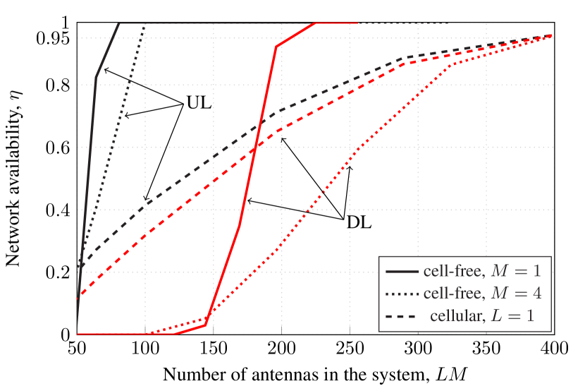
Figure 1: Network availability for $\epsilon_{\text{{}target}}=10^{-5}$ with MMSE combining/precoding as a function of the total number of antennas in the system $LM$. Here, $K=40$, $n_{\text{{}p}}=40$, $\Delta=25^{\circ}$, the scenario size is $150\times 150$ m, $\rho^{\mathrm{ul}}=\rho^{\mathrm{dl}}=-10\,\mathrm{dBm}$, $\log_{2}m=160$, and $n=300$.

For the case of MMSE channel estimation with MMSE combining/precoding (Fig. 1), a network availability above $0.95$ in both UL and DL is obtained in the cell-free setting with $L=200$ single-antenna APs ($M=1$). Increasing the number of antennas per AP does not seem to help even in the DL, where channel hardening is expected to improve as $M$ grows [15]. Indeed, although channel hardening improves, larger pathlosses due to smaller AP densities may have a bigger impact on the DL error probability. For example, when $M=4$, the cell-free setting requires $L=100$ APs ($LM=400$) to achieve $\eta\geq 0.95$ in both UL and DL. The cellular network requires a total number of $M=400$ antennas to achieve $\eta=0.95$. This illustrates the superiority of the cell-free architecture in providing URLLC services.

In all the cases considered in Fig. 1, the DL limits the performance. This is because the UEs have no CSI and perform mismatched decoding by relying on channel hardening. For example, in the cell-free setting with $M=1$, the UL requires only $L=81$ to reach $\eta=1$. However, the DL requires $L=225$ to reach $\eta=1$.

It is interesting to note that for both UL and DL, the network availability exhibits a much sharper transition from low values to high values in the cell-free setting than in the cellular setting. This is particularly evident for the DL, where $\eta$ goes from around $0.05$ to around $0.95$ as $L$ is increased from $150$ to $200$. For the same number of antennas, $\eta$ increases from $0.46$ to $0.64$ with cellular Massive MIMO.

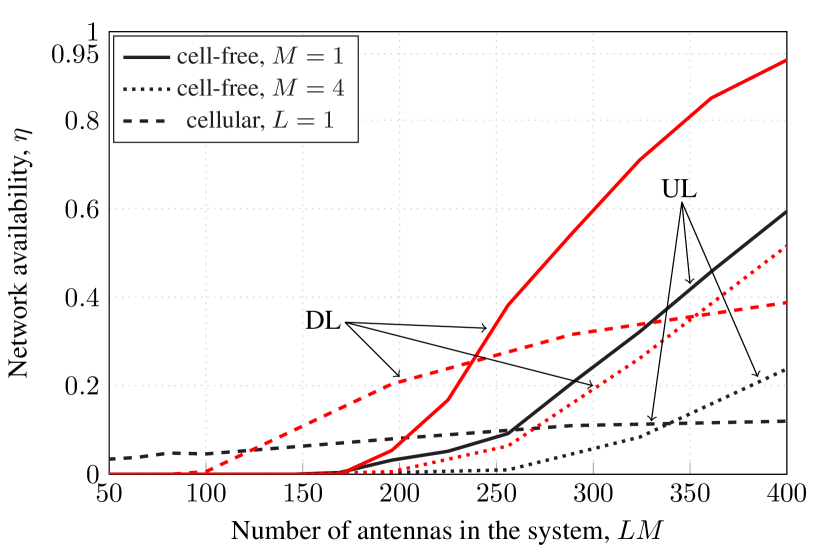
Figure 2: Network availability for $\epsilon_{\text{{}target}}=10^{-5}$ with MR combining/precoding in the same setup of Fig. 1.

With MR combining/precoding (Fig. 2), a network availability close to $0.95$ can be achieved in the DL of the cell-free setting with single-antenna APs only when $L=400$. Note that, with this number of APs, the DL outperforms the UL. This phenomenon, which was previously noted in [10, Sec. III-D] in the context of cellular Massive MIMO and URLLC services, is due to two reasons:

1. The number of APs is sufficiently large for channel hardening to occur.

2. MR combining/precoding maximizes the array gain without mitigating the interference, which implies that when the desired signal experiences a deep fade, the magnitude of the UL interference is unaffected. On the contrary, when the desired signal experiences a deep fade, the DL interference becomes small, too. This results in a larger error probability in the UL compared to the DL. This phenomenon, however, does not occur when MMSE combining/precoding is used. A more detailed discussion can be found in [10, Sec. III-D].

Finally, it is worth highlighting that if cooperation between APs is not allowed in the cell-free network—a scenario referred to in [7] as “level-1 cooperation: small-cell network”, the network availability is zero when using APs with both $M=1$ and $M=4$ for the system parameters considered in Fig. 1 and Fig. 2. Thus, allowing the APs to cooperate is crucial when deploying a cell-free network intended to support URLLC.

V Conclusions

We analyzed a cell-free Massive MIMO system supporting URLLC services, in terms of network availability. Numerical results, based on a saddlepoint approximation of the RCUs bound (stated in Theorem 1) on the per-user UL and DL error probabilities, revealed that, in an automated-factory scenario, cell-free Massive MIMO with fully centralized processing outperforms cellular Massive MIMO. The analysis revealed also the importance of using MMSE linear processing in place of MR processing to obtain satisfactory performance. Furthermore, it was illustrated that, when the UEs have no CSI and rely on channel hardening, the DL is typically the bottleneck from a system performance perspective, and deploying a sufficiently large number of APs, so as to achieve a critical AP density, is crucial. It turned out that, for a given total number of antennas, it is more beneficial to deploy many single-antennas APs, than fewer multiple-antenna APs.

References

- [1] E. Björnson, L. Sanguinetti, H. Wymeersch, J. Hoydis, and T. L. Marzetta, “Massive MIMO is a reality—what is next?: Five promising research directions for antenna arrays,” Digital Signal Processing, vol. 94, pp. 3–20, Nov. 2019.
- [2] L. Sanguinetti, E. Björnsson, and J. Hoydis, “Towards massive MIMO 2.0: Understanding spatial correlation, interference suppression, and pilot contamination,” IEEE Trans. Commun., vol. 68, no. 1, pp. 232–257, Jan. 2020.
- [3] H. Q. Ngo, A. Ashikhmin, H. Yang, E. G. Larsson, and T. L. Marzetta, “Cell-free massive MIMO versus small cells,” IEEE Trans. Wireless Commun., vol. 16, no. 3, pp. 1834–1850, Mar. 2017.
- [4] E. Nayebi, A. Ashikhmin, T. L. Marzetta, H. Yang, and B. D. Rao, “Precoding and power optimization in cell-free Massive MIMO systems,” IEEE Trans. Wireless Commun., vol. 16, no. 7, pp. 4445–4459, Jul. 2017.
- [5] 3GPP, “Service requirements for cyber-physical control applications in vertical domains,” 3rd Generation Partnership Project (3GPP), Technical Specification (TS) 22.104, 12 2019, version 17.2.0.
- [6] G. Durisi, T. Koch, and P. Popovski, “Towards massive, ultra-reliable, and low-latency wireless communication with short packets,” Proc. IEEE, vol. 104, no. 9, pp. 1711–1726, Sep. 2016.
- [7] E. Björnson and L. Sanguinetti, “Making cell-free Massive MIMO competitive with MMSE processing and centralized implementation,” IEEE Trans. Wireless Commun., vol. 19, no. 1, pp. 77–90, Jan. 2020.
- [8] A. A. Nasir, H. D. Tuan, H. Q. Ngo, T. Q. Duong, and H. V. Poor, “Cell-free massive MIMO in the short blocklength regime for URLLC,” IEEE Trans. Wireless Commun., Apr. 2021, (early access).
- [9] Y. Polyanskiy, H. V. Poor, and S. Verdú, “Channel coding rate in the finite blocklength regime,” IEEE Trans. Inf. Theory, vol. 56, no. 5, pp. 2307–2359, May 2010.
- [10] J. Östman, A. Lancho, G. Durisi, and L. Sanguinetti, “URLLC with Massive MIMO: Analysis and design at finite blocklength,” IEEE Trans. Wireless Commun., 2021.
- [11] J. Östman, G. Durisi, E. G. Ström, M. C. Coskun, and G. Liva, “Short packets over block-memoryless fading channels: Pilot-assisted or noncoherent transmission?” IEEE Trans. Commun., vol. 67, no. 2, pp. 1521–1536, Feb. 2019.
- [12] A. Martinez and A. Guillén i Fàbregas, “Saddlepoint approximation of random–coding bounds,” in Proc. Inf. Theory Applicat. Workshop (ITA), San Diego, CA, USA, Feb. 2011.
- [13] W. Feller, An Introduction to Probability Theory and Its Applications, 2nd ed. New York, NY, USA: Wiley, 1971, vol. II.
- [14] E. Björnson, J. Hoydis, and L. Sanguinetti, “Massive MIMO Networks: Spectral, Energy, and Hardware Efficiency,” Foundations and Trends® in Signal Processing, vol. 11, no. 3-4, pp. 154–655, Nov. 2017.
- [15] Z. Chen and E. Björnson, “Channel hardening and favorable propagation in cell-free Massive MIMO with stochastic geometry,” IEEE Trans. on Commun., vol. 66, no. 11, pp. 5205–5219, Jun. 2018.