h FR-PHENO-2021-08, VBSCAN-PUB-06-21
Full NLO predictions for vector-boson scattering into Z bosons and its irreducible background at the LHC

Abstract

Vector-boson scattering into two Z bosons at the LHC is a key channel for the exploration of the electroweak sector of the Standard Model. It allows for the full reconstruction of the scattering process but at the price of a huge irreducible background. For the first time, we present full next-to-leading-order predictions for $\text{p}\text{p}\to\text{e}^{+}\text{e}^{-}\mu^{+}\mu^{-}\text{j}\text{j}+X$ including all electroweak and QCD contributions for vector-boson scattering signal and irreducible background. The results are presented in the form of cross sections and differential distributions. A particular emphasis is put on the newly computed $\mathcal{O}{\left(\alpha_{\text{s}}^{2}\alpha^{5}\right)}$ corrections.

1 Introduction

An important part of the physics programme conducted at the Large Hadron Collider (LHC) aims at extracting Standard Model parameters by measuring precisely particular processes. This requires the definition of tailored event selections and the subtraction of undesirable background processes. In the presence of irreducible backgrounds, this picture gets complicated through non-vanishing interferences between the signal and background processes. For vector-boson scattering (VBS), the irreducible background can be overwhelming which warrants a detailed analysis of both the signal and background in order to fully exploit its physics potential Covarelli:2021gyz ; 1866947 .

The present article continues a series of studies Biedermann:2016yds ; Biedermann:2017bss ; Denner:2019tmn ; Denner:2020zit aiming at describing not only VBS processes but also their irreducible backgrounds with next-to-leading-order (NLO) accuracy. Given that the signal and background are connected through interferences, a physical definition of a signal and background separately is not possible (even when using exclusive cuts to enhance the electroweak (EW) component). At NLO, the situation becomes even more complicated as a separation of signal and background in an IR-finite way must necessarily rely on approximations Ballestrero:2018anz .

On top of these considerations, there are more pragmatic reasons to investigate in detail both the EW and QCD components of VBS at full NLO accuracy. While for the same-sign W channel the signal-to-background ratio is about $8/1$, it is only of the order of $1/2$ for the ZZ case. In addition, given the smallness of the cross sections it is critical to know all contributions, including the loop-induced contribution.

Important steps towards describing $\text{p}\text{p}\to\text{e}^{+}\text{e}^{-}\mu^{+}\mu^{-}\text{j}\text{j}+X$ at full NLO accuracy have already been taken, especially regarding NLO QCD corrections. These are known for the EW component Jager:2006cp in the VBS approximation and have been implemented in the POWHEG BOX framework Alioli:2010xd to also include parton-shower (PS) corrections Jager:2013iza . In addition, NLO QCD corrections to the QCD component are known Campanario:2014ioa and can in principle be obtained at NLO QCD+PS accuracy from public multi-purpose Monte Carlo generators such as MadGraph5_aMC@NLO Alwall:2014hca or Sherpa Sherpa:2019gpd . The full NLO corrections of orders $\mathcal{O}{\left(\alpha^{7}\right)}$ and $\mathcal{O}{\left(\alpha_{\text{s}}\alpha^{6}\right)}$ have been computed in Ref. Denner:2020zit along with the loop-induced contribution of order $\mathcal{O}{\left(\alpha_{\text{s}}^{4}\alpha^{4}\right)}$. Finally, in Ref. Li:2020nmi , results for loop-induced ZZ production with up to 2 jets merged and matched to parton showers have been presented. Therefore, at NLO level the only missing piece is the order $\mathcal{O}{\left(\alpha_{\text{s}}^{2}\alpha^{5}\right)}$, which is for simplicity sometimes referred to as EW corrections to the QCD component in the following. With the present publication we fill this gap by presenting for the first time the full NLO corrections to $\text{p}\text{p}\to\text{e}^{+}\text{e}^{-}\mu^{+}\mu^{-}\text{j}\text{j}+X$ at the LHC in a unique setup.

Previous works Biedermann:2016yds ; Biedermann:2017bss ; Denner:2019tmn ; Denner:2020zit have put a strong emphasis on EW corrections of order $\mathcal{O}{\left(\alpha^{7}\right)}$. These are exceptionally large for EW corrections and are an intrinsic feature of VBS at the LHC Biedermann:2016yds . They are even the largest NLO contribution for the same-sign WW (ss-WW) channel which has thus motivated their implementation in the POWHEG BOX Chiesa:2019ulk . Such a hierarchy of the NLO contributions is not only due to the general characteristics of VBS but also to the large signal-over-background ratio in the ss-WW channel. In other cases, like for vector-boson scattering into ZZ where the background is large, such a hierarchy does not necessarily hold. In this article we study these implications and give new insights in VBS and its irreducible background at the LHC.

The results presented in this article should be of great interest for experimental collaborations. In particular, the ATLAS and CMS collaborations have already observed the EW ZZjj production Aad:2020zbq ; Sirunyan:2017fvv ; Sirunyan:2020alo . Along with state-of-the-art theoretical predictions, upcoming data will allow for deeper analyses of VBS at the LHC.

This article is structured as follows: In Section 2 the process under consideration is introduced. In Section 3 the results are presented and analysed in detail. Finally, Section 4 contains a summary and concluding remarks.

2 Description of the calculation

The present article complements Ref. Denner:2020zit by providing the two missing NLO contributions of orders $\mathcal{O}{\left(\alpha_{\text{s}}^{2}\alpha^{5}\right)}$ and $\mathcal{O}{\left(\alpha_{\text{s}}^{3}\alpha^{4}\right)}$. Therefore, in the following, we often refer to this reference, and the interested reader is invited to look into it. For the sake of simplicity some information is not repeated here as we focus on the salient features of the newly computed contributions.

2.1 The process

The physical process under investigation is

$$\text{p}\text{p}\to\text{e}^{+}\text{e}^{-}\mu^{+}\mu^{-}\text{j}\text{j}+X$$ (1)

at the LHC. In the same way as all processes containing VBS contributions, its cross section possesses three leading-order (LO) components: an EW one of order $\mathcal{O}{\left(\alpha^{6}\right)}$ including VBS, an interference of order $\mathcal{O}{\left(\alpha_{\text{s}}\alpha^{5}\right)}$, and a QCD contribution of order $\mathcal{O}{\left(\alpha^{2}_{\rm s}\alpha^{4}\right)}$. Exemplary Feynman diagrams of order $\mathcal{O}{\left({g}^{6}\right)}$ and $\mathcal{O}{\left({g}^{2}_{\rm s}{g}^{4}\right)}$ are shown in Fig. 1.

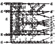
(a)

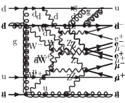
(b)

(c)

Figure 1: Examples of tree-level Feynman diagrams: EW (left) and QCD (middle and right).

At order $\mathcal{O}{\left({g}^{2}_{\rm s}{g}^{4}\right)}$, besides partonic processes involving four quarks, also processes with two quarks and two gluons appear (see Fig. 1(c)) with all possible crossings of gluons and quarks.

At NLO, there are four orders contributing: $\mathcal{O}{\left(\alpha^{7}\right)}$, $\mathcal{O}{\left(\alpha_{\text{s}}\alpha^{6}\right)}$, $\mathcal{O}{\left(\alpha^{2}_{\rm s}\alpha^{5}\right)}$, and $\mathcal{O}{\left(\alpha^{3}_{\rm s}\alpha^{4}\right)}$. The first two have been computed without approximations in Ref. Denner:2020zit . The latter has been evaluated in Ref. Campanario:2014ioa , while the order $\mathcal{O}{\left(\alpha^{2}_{\rm s}\alpha^{5}\right)}$ is calculated here for the first time. Given that the first two orders are discussed in detail in Ref. Denner:2020zit , the discussion in the following is focused on the two remaining orders, which receive contributions from partonic processes involving four quarks as well as from those with two quarks and gluons.

The order $\mathcal{O}{\left(\alpha^{2}_{\rm s}\alpha^{5}\right)}$ is made of corrections of both QCD and EW types [as the order $\mathcal{O}{\left(\alpha_{\text{s}}\alpha^{6}\right)}$]. In particular, it features both types of real corrections: photon emissions and emissions of QCD partons. The first contribution entails squared matrix elements of photon-emission diagrams of order $\mathcal{O}{\left({g}^{2}_{\rm s}{g}^{5}\right)}$ as shown in Fig. 2(a). The second one is made of interferences of QCD real matrix elements of orders $\mathcal{O}{\left({g}_{\rm s}{g}^{6}\right)}$ (shown in Fig. 2(b)) and $\mathcal{O}{\left({g}^{3}_{\rm s}{g}^{4}\right)}$ (shown in Fig. 2(c)).

(a)

(b)

(c)

Figure 2: Examples of real tree-level Feynman diagrams: photon emission (left) and gluon emission off LO EW (middle) and QCD diagrams (right).

Their infrared (IR) singularities are compensated by the corresponding virtual corrections, which also receive two types of contributions. The first one consists of one-loop amplitudes of order $\mathcal{O}{\left({g}^{2}_{\rm s}{g}^{6}\right)}$ (as shown in Fig. 3(a)) interfered with tree-level amplitudes of order $\mathcal{O}{\left({g}^{2}_{\rm s}{g}^{4}\right)}$ (Fig. 1(b)).

(a)

(b)

(c)

Figure 3: Examples of virtual one-loop Feynman diagrams: mixed EW–QCD loop (left) and purely QCD loops (middle and right).

The second type is furnished by one-loop amplitudes of order $\mathcal{O}{\left({g}^{4}_{\rm s}{g}^{4}\right)}$ (as shown in Figs. 3(b)) interfered with tree-level amplitudes of order $\mathcal{O}{\left({g}^{6}\right)}$ (Fig. 1(a)). We note that the two types of NLO corrections cannot be defined in an IR-finite way on the basis of Feynman diagrams in a full computation Biedermann:2017bss , i.e. without relying on any approximations Ballestrero:2018anz . For instance, the diagram in Fig. 3(a) can be viewed as an EW correction to a LO diagram of order $\mathcal{O}{\left({g}^{2}_{\rm s}{g}^{4}\right)}$ or as a QCD correction to a LO diagram of order $\mathcal{O}{\left(g^{6}\right)}$.

As explained above, at the order $\mathcal{O}{\left(\alpha^{2}_{\rm s}\alpha^{5}\right)}$, some of the real corrections are made of a photon emission of a LO QCD amplitude. It also means that in the final state one can have a photon as well as one (or two) gluon(s). In the case where a hard photon is recombined with a soft gluon in a single jet, the QCD singularity associated to the soft gluon is not accounted for by the QED subtraction term. To avoid such configurations, a veto is typically applied on jets that have a too large photon–jet energy fraction

$$z_{\gamma}=\frac{E_{\gamma}}{E_{\gamma}+E_{a}},$$ (2)

where $E_{\gamma}$ and $E_{a}$ are the energy of the photon and the QCD parton $a$, respectively. In the present case, the numerical limit has been chosen to be $z_{\gamma}<z_{\gamma,\rm cut}=0.7$. By cutting into the collinear region, IR-safety is lost but can be restored upon including the nonperturbative fragmentation of quarks into photons via the fragmentation function Denner:2009gj ; Denner:2010ia ; Denner:2011vu ; Denner:2014ina . Schematically, the NLO cross section in the relevant order can be written as

$$\mathrm{d}\sigma_{\rm NLO}= \int_{n+1}\theta(z_{\gamma,\rm cut}-z_{\gamma})\left[\mathrm{d}\sigma_{\rm real}-\mathrm{d}\sigma_{\rm dipole}\right]+$$

$$\int_{n}\left[\mathrm{d}\sigma_{\rm virtual}+\int_{1}\left(\mathrm{d}\sigma_{\rm dipole}-\mathrm{d}\sigma^{\gamma\;\rm coll}_{\rm dipole}(z_{\gamma,\rm cut})\right)-\mathrm{d}\sigma_{\rm frag}(z_{\gamma,\rm cut})\right],$$ (3)

where the index at the integrals denotes the number of particles in the corresponding phase spaces. The modification of the dipoles due to the rejection of hard photons is thus encoded in

$$\mathrm{d}\sigma^{\gamma\;\rm coll}_{\rm frag}(z_{\gamma,\rm cut})=\theta(z_{\gamma}-z_{\gamma,\rm cut})\mathrm{d}\sigma_{\rm dipole}.$$ (4)

In addition, the contributions of final-state quarks fragmenting into a hard photon are accounted for by

$$\mathrm{d}\sigma_{\rm frag}(z_{\gamma,\rm cut})=\sum_{i}\mathrm{d}\sigma_{\rm Born}\int^{1}_{z_{\gamma},\rm cut}\mathrm{d}z_{\gamma}\,D_{q_{i}\to\gamma}(z_{\gamma}),$$ (5)

where the sum runs over all the final state quarks and $D_{q_{i}\to\gamma}$ is the quark-to-photon fragmentation function.

For the present computation, the fit parameters entering the fragmentation function have been taken from Ref. Buskulic:1995au and read

$$\mu_{0}=0.14\,\text{GeV},\qquad C=-13.26.$$ (6)

Finally, the order $\mathcal{O}{\left(\alpha^{3}_{\rm s}\alpha^{4}\right)}$ is made of NLO QCD corrections only. This means that it contains squares of amplitudes with a gluon attached to the $\mathcal{O}{\left({g}^{2}_{\rm s}{g}^{4}\right)}$ diagrams as shown in Fig. 2(c), furnishing the real corrections of order $\mathcal{O}{\left(\alpha^{3}_{\rm s}\alpha^{4}\right)}$. The virtual contributions are made of one-loop amplitudes of order $\mathcal{O}{\left({g}^{4}_{\rm s}{g}^{4}\right)}$ (as shown in Figs. 3(b) and 3(c)) interfered with tree-level amplitudes of order $\mathcal{O}{\left({g}^{2}_{\rm s}{g}^{4}\right)}$ (Fig. 1(b)).

Note that we do not consider contributions with external bottom quarks in any of the LO or NLO contributions. These are small or can be removed in experimental analyses with the help of bottom-jet vetoes Denner:2019tmn ; Denner:2020zit .

2.2 Details and validation

The results presented here have been produced using the Monte Carlo program MoCaNLO and the matrix-element generator Recola. The program MoCaNLO is able to compute arbitrary processes within the SM at NLO QCD and EW accuracy. In order to obtain a fast integration for high-multiplicity processes with many resonances, it takes advantage of phase-space mappings similar to the ones of Refs. Berends:1994pv ; Denner:1999gp ; Dittmaier:2002ap . On the other hand, Recola Actis:2012qn ; Actis:2016mpe is a general tree and one-loop matrix-element provider. It relies on the Collier library Denner:2014gla ; Denner:2016kdg that provides numerically the one-loop scalar 'tHooft:1978xw ; Beenakker:1988jr ; Dittmaier:2003bc ; Denner:2010tr and tensor integrals Passarino:1978jh ; Denner:2002ii ; Denner:2005nn . This combination has already shown to work well for high-multiplicity processes ($2\to 6$ and beyond). Many of these applications concerned VBS processes Biedermann:2016yds ; Biedermann:2017bss ; Ballestrero:2018anz ; Denner:2019tmn ; Pellen:2019ywl ; Denner:2020zit . During the course of these studies, the set of tools was verified against BONSAY+O PEN L OOPS Denner:2019tmn for WZ scattering, the Monte Carlo BBMC for same-sign W scattering Biedermann:2016yds ; Biedermann:2017bss , and against Powheg Chiesa:2019ulk for same-sign W scattering at order $\mathcal{O}{\left(\alpha^{7}\right)}$. For non-VBS processes, it was checked against Sherpa in Refs. Biedermann:2017yoi ; Brauer:2020kfv and a multitude of tools in Ref. Bendavid:2018nar for di-boson production at NLO EW.

Finally, in Ref. Denner:2020zit , the partonic processes $\text{u}\text{d}\to\text{e}^{+}\text{e}^{-}\mu^{+}\mu^{-}\text{u}\text{d}$, $\text{u}\text{s}\to\text{e}^{+}\text{e}^{-}\mu^{+}\mu^{-}\text{d}\text{c}$, $\text{u}\text{u}\to\text{e}^{+}\text{e}^{-}\mu^{+}\mu^{-}\text{u}\text{u}$, and $\text{u}\bar{}\text{c}\to\text{e}^{+}\text{e}^{-}\mu^{+}\mu^{-}\text{d}\bar{}\text{s}$ at order $\mathcal{O}{\left(\alpha^{7}\right)}$ were successfully compared between MoCaNLO+Recola and BBMC+Recola. Also, selected contributions of order $\mathcal{O}{\left(\alpha_{\text{s}}\alpha^{6}\right)}$ were found in agreement within integration errors. For the present article, about 10 representative partonic channels were confirmed to agree between MoCaNLO and BBMC at the NLO orders $\mathcal{O}{\left(\alpha^{2}_{\rm s}\alpha^{5}\right)}$ and $\mathcal{O}{\left(\alpha^{3}_{\rm s}\alpha^{4}\right)}$ within statistical errors at the level of a few per cent.

In MoCaNLO and BBMC, the subtraction of IR divergences in the real radiation is realised with the help of the Catani–Seymour dipole formalism Catani:1996vz ; Dittmaier:1999mb ; Dittmaier:2008md . Within this method, it is possible to vary the $\alpha_{\mathrm{dipole}}$ parameter Nagy:1998bb , which restricts the subtraction to IR-singular regions of the phase space. Obtaining consistent results with different values $\alpha_{\mathrm{dipole}}$ ensures the correctness of the subtraction mechanism. We have therefore performed two full computations of all NLO orders using MoCaNLO+Recola with $\alpha_{\mathrm{dipole}}=1$ and $\alpha_{\mathrm{dipole}}=10^{-2}$. Full statistical agreement has been found, and the results presented here are the ones obtained with $\alpha_{\mathrm{dipole}}=10^{-2}$. Also, for the computation of order $\mathcal{O}{\left(\alpha^{2}_{\rm s}\alpha^{5}\right)}$ two different modes of Collier have been successfully compared. The results presented here have been obtained with the COLI mode throughout. In all computations, the complex-mass scheme Denner:1999gp ; Denner:2005fg ; Denner:2006ic ; Denner:2019vbn is utilised.

Finally, the implementation of the fragmentation function closely follows Refs. Denner:2009gj ; Denner:2010ia ; Denner:2011vu ; Denner:2014ina . Its implementation in MoCaNLO has been validated against BBMC which was used in Ref. Denner:2014ina for the computation of the EW corrections to $\text{p}\text{p}\to\ell^{+}\ell^{-}\text{j}\text{j}+X$. Also, this implementation was employed in Ref. Brauer:2020kfv for $\text{p}\text{p}\to\text{e}^{+}\nu_{\text{e}}\mu^{-}\bar{\nu}_{\mu}\text{j}+X$ where it was compared against an approximate treatment.

3 Numerical results

3.1 Input parameters and event selection

The input parameters and event selection used in the present article are exactly the same as those in Ref. Denner:2020zit . For completeness we reproduce them here.

Input parameters

The calculation is done for LHC characteristics and a centre-of-mass energy of $13\,\text{TeV}$. The set of parton distribution functions (PDF) NLO NNPDF-3.1 Lux QED with $\alpha_{\text{s}}(M_{\text{Z}})=0.118$ Ball:2014uwa ; Bertone:2017bme and with fixed $N_{\text{F}}=5$ flavour scheme is used throughout. All collinear initial-state splittings are treated by the ${\overline{\rm MS}}$ redefinition of the PDF. The PDF set is interfaced to our Monte Carlo programs using LHAPDF Andersen:2014efa ; Buckley:2014ana .

The renormalisation and factorisation scales, $\mu_{\rm ren}$ and $\mu_{\rm fac}$, are chosen to be

$$\mu_{0}=\sqrt{p_{{\mathrm{T}},\text{j}_{1}}\,p_{{\mathrm{T}},\text{j}_{2}}}$$ (7)

for all contributions, where $\text{j}_{1}$ and $\text{j}_{2}$ are the two hardest (in $p_{\rm T}$) identified jets (tagging jets). This is the scale choice that is usually used for VBS processes in the literature and that has been also employed in Ref. Denner:2020zit . In cross sections and differential distributions, the scale uncertainty is obtained with the standard 7-point scale variation, i.e. observables are evaluated for the 7 pairs of renormalisation and factorisation scales

$$(\mu_{\mathrm{ren}}/\mu_{0},\mu_{\mathrm{fact}}/\mu_{0})=(0.5,0.5),(0.5,1),(1,0.5),(1,1),(1,2),(2,1),(2,2),$$ (8)

and the scale variation is determined from the resulting envelope.

The electromagnetic coupling is obtained through the $G_{\mu}$ scheme Denner:2000bj via

$$\alpha=\frac{\sqrt{2}}{\pi}G_{\mu}M_{\text{W}}^{2}\left(1-\frac{M_{\text{W}}^{2}}{M_{\text{Z}}^{2}}\right)\qquad\text{with}\qquad{G_{\mu}=1.16638\times 10^{-5}\,\text{GeV}^{-2}},$$ (9)

where $G_{\mu}$ is the Fermi constant. The numerical values of the masses and widths used as input in the numerical simulation read ParticleDataGroup:2020ssz

$$m_{\text{t}} =173.0\,\text{GeV}, \quad\quad\quad\Gamma_{\text{t}} =0\,\text{GeV},$$

$$M_{\text{Z}}^{\text{OS}} =91.1876\,\text{GeV}, \quad\quad\quad\Gamma_{\text{Z}}^{\text{OS}} =2.4952\,\text{GeV},$$

$$M_{\text{W}}^{\text{OS}} =80.379\,\text{GeV}, \Gamma_{\text{W}}^{\text{OS}} =2.085\,\text{GeV},$$

$$M_{\rm H} =125.0\,\text{GeV}, \Gamma_{\text{H}} =4.07\times 10^{-3}\,\text{GeV}.$$ (10)

Everywhere, it is assumed that $m_{\text{b}}=0\,\text{GeV}$ and as mentioned above no partonic channels with external bottom quarks are considered. For the massive gauge bosons (W and Z), the pole masses and widths utilised in the calculation are obtained from the on-shell (OS) values Bardin:1988xt using

$$M_{V}=\frac{M_{V}^{\text{OS}}}{\sqrt{1+(\Gamma_{V}^{\text{OS}}/M_{V}^{\text{OS}})^{2}}}\,,\qquad\Gamma_{V}=\frac{\Gamma_{V}^{\text{OS}}}{\sqrt{1+(\Gamma_{V}^{\text{OS}}/M_{V}^{\text{OS}})^{2}}}.$$ (11)

Event selection

The event selection of the present computation is largely inspired from the CMS analyses Sirunyan:2017fvv ; Sirunyan:2020alo . The process features four charged leptons and two jets in the final state. Quarks and gluons with pseudorapidity $|\eta|<5$ are clustered into jets with the anti-$k_{{\mathrm{T}}}$ algorithm Cacciari:2008gp using $R=0.4$. Following the same method and radius parameter, the photons are recombined with the final-state jets or leptons.

The four leptons $\ell$ must fulfil

$$p_{\text{T},\ell}>20\,\text{GeV},\qquad|\eta_{\ell}|<2.5,\qquad\Delta R_{\ell\ell^{\prime}}>0.05,\qquad M_{\ell^{+}\ell^{\prime-}}>4\,\text{GeV},$$ (12)

where $\ell$ and $\ell^{\prime}$ are any leptons while $\ell^{+}$ and $\ell^{\prime-}$ are oppositely charged leptons regardless of their flavour. On top of these cuts, the invariant masses of the leptonic decay products of the Z bosons are restricted to

$$60\,\text{GeV}<M_{\ell^{+}\ell^{-}}<120\,\text{GeV},\qquad\ell=\text{e},\mu.$$ (13)

Once the jet clustering is performed, at least two jets still have to fulfil the criteria

$$p_{\text{T},\text{j}}>30\,\text{GeV},\qquad|\eta_{\text{j}}|<4.7,\qquad\Delta R_{\text{j}\ell}>0.4.$$ (14)

Such jets are then denoted as identified jets. Out of these, the two with the highest transverse momenta are called tagging jets.

In our default setup (inclusive setup for short) the tagging jets have to fulfil the constraint

$$M_{\text{j}_{1}\text{j}_{2}}>100\,\text{GeV}.$$ (15)

We consider in addition a setup (VBS setup) where the last cut is replaced by a stronger one

$$M_{\text{j}_{1}\text{j}_{2}}>500\,\text{GeV}.$$ (16)

3.2 Cross sections

In this section, various cross sections at LO and NLO accuracy are discussed. We start by recalling the LO cross sections computed in Ref. Denner:2020zit in Table 1.

Order	$\mathcal{O}{\left(\alpha^{6}\right)}$	$\mathcal{O}{\left(\alpha_{\text{s}}\alpha^{5}\right)}$	$\mathcal{O}{\left(\alpha_{\text{s}}^{2}\alpha^{4}\right)}$	Sum	$\mathcal{O}{\left(\alpha_{\text{s}}^{4}\alpha^{4}\right)}$
$M_{\text{j}_{1}\text{j}_{2}}>100\,\text{GeV}$
$\sigma_{\mathrm{LO}}^{4q}[$\mathrm{fb}$]$	$0.097683(2)$	$0.008628(1)$	$0.22138(1)$	$0.32770(1)$	-
$\sigma_{\mathrm{LO}}^{2q2\text{g}}[$\mathrm{fb}$]$	-	-	$0.84122(5)$	$0.84122(5)$	$0.1210(6)$
$\sigma_{\mathrm{LO}}[$\mathrm{fb}$]$	$0.097683(2)$	$0.008628(1)$	$1.06260(5)$	$1.16891(5)$	$0.1210(6)$
$\textrm{fraction}[$\mathrm{\char 37\relax}$]$	$8.36$	$0.74$	$90.91$	$100$	$10.35$
$M_{\text{j}_{1}\text{j}_{2}}>500\,\text{GeV}$
$\sigma_{\mathrm{LO}}^{4q}[$\mathrm{fb}$]$	$0.073676(3)$	$0.005567(1)$	$0.046230(4)$	$0.125470(4)$	-
$\sigma_{\mathrm{LO}}^{2q2\text{g}}[$\mathrm{fb}$]$	-	-	$0.08992(2)$	$0.08992(2)$	$0.0135(3)$
$\sigma_{\mathrm{LO}}[$\mathrm{fb}$]$	$0.073676(3)$	$0.005567(1)$	$0.13614(2)$	$0.21539(2)$	$0.0135(3)$
$\textrm{fraction}[$\mathrm{\char 37\relax}$]$	$34.21$	$2.58$	$63.21$	$100$	$6.24$

Table 1: LO cross section of the individual orders $\mathcal{O}{\left(\alpha^{6}\right)}$, $\mathcal{O}{\left(\alpha_{\text{s}}\alpha^{5}\right)}$, $\mathcal{O}{\left(\alpha_{\text{s}}^{2}\alpha^{4}\right)}$, and their sum for $\text{p}\text{p}\to\text{e}^{+}\text{e}^{-}\mu^{+}\mu^{-}\text{j}\text{j}+X$ at $13\,\text{TeV}$ CM energy. Contributions of partonic channels with four external quarks, $\sigma_{\mathrm{LO}}^{4q}$, and those with two external quarks and two external gluons, $\sigma_{\mathrm{LO}}^{2q2\text{g}}$, are shown separately as well. The loop-induced contribution of $\mathcal{O}{\left(\alpha_{\text{s}}^{4}\alpha^{4}\right)}$ is also listed but does not enter the sum of contributions. Each contribution is given in  fb and as fraction relative to the sum of the three contributions (in per cent). While the numbers in the upper part of the table are for the inclusive setup, those in the lower part are for the VBS setup. The digits in parentheses indicate integration errors.

As opposed to Ref. Denner:2020zit , here the sum comprises only the contributions of orders $\mathcal{O}{\left(\alpha^{6}\right)}$, $\mathcal{O}{\left(\alpha_{\text{s}}\alpha^{5}\right)}$, and $\mathcal{O}{\left(\alpha_{\text{s}}^{2}\alpha^{4}\right)}$, while the loop-induced contribution of order $\mathcal{O}{\left(\alpha_{\text{s}}^{4}\alpha^{4}\right)}$ from $\text{g}\text{g}\to\text{e}^{+}\text{e}^{-}\mu^{+}\mu^{-}\text{g}\text{g}$ does not enter the sum and is only shown for completeness. Contributions of partonic channels with four external quarks, $\sigma_{\mathrm{LO}}^{4q}$, and of those involving gluons, $\sigma_{\mathrm{LO}}^{2q2\text{g}}$, which enter at order $\mathcal{O}{\left(\alpha_{\text{s}}^{2}\alpha^{4}\right)}$, are shown separately as well. When referring to relative corrections in the following, they are always normalised to the above LO sum, and the loop-induced contribution is not included in the NLO predictions. Table 1 clearly shows that the QCD contribution of order $\mathcal{O}{\left(\alpha_{\text{s}}^{2}\alpha^{4}\right)}$ is dominating and reaches $91\%$ of the LO sum for $M_{\text{j}_{1}\text{j}_{2}}>100\,\text{GeV}$. When applying the tighter VBS event selection, $M_{\text{j}_{1}\text{j}_{2}}>500\,\text{GeV}$, it is reduced to $63\%$, demonstrating hence the impact of such cuts in enhancing the EW contribution. While the partonic channels involving quarks and gluons contribute $79\%$ at $\mathcal{O}{\left(\alpha_{\text{s}}^{2}\alpha^{4}\right)}$ and $72\%$ of the LO sum for the inclusive case, their share is diminished to $66\%$ and $42\%$, respectively, for the VBS setup. The tighter VBS cuts also reduce the relative contribution of the loop-induced process from $10\%$ down to $6\%$. Including 7-point scale variations, the full LO cross section comprising the orders $\mathcal{O}{\left(\alpha^{6}\right)}$, $\mathcal{O}{\left(\alpha_{s}\alpha^{5}\right)}$, and $\mathcal{O}{\left(\alpha_{\text{s}}^{2}\alpha^{4}\right)}$ reads

$$\sigma_{\textrm{LO}}={} 1.16879(5)^{+29.1\%}_{-20.7\%}\qquad\text{ for }\quad M_{\text{j}_{1}\text{j}_{2}}>100\,\text{GeV},$$

$$\sigma_{\textrm{LO}}={} 0.21539(2)^{+26.0\%}_{-18.3\%}\qquad\text{ for }\quad M_{\text{j}_{1}\text{j}_{2}}>500\,\text{GeV}.$$ (17)

With $30\%$ the LO scale dependence has the typical order of magnitude for a cross section of order $\mathcal{O}{\left(\alpha_{\text{s}}^{2}\right)}$. It is somewhat reduced for $M_{\text{j}_{1}\text{j}_{2}}>500\,\text{GeV}$ owing to the larger fraction of the EW contribution.

The full NLO cross section, including orders $\mathcal{O}{\left(\alpha^{7}\right)}$, $\mathcal{O}{\left(\alpha_{\text{s}}\alpha^{6}\right)}$, $\mathcal{O}{\left(\alpha_{\text{s}}^{2}\alpha^{5}\right)}$, and $\mathcal{O}{\left(\alpha_{\text{s}}^{3}\alpha^{4}\right)}$, reads with 7-point scale variations

$$\sigma_{\textrm{NLO}}={} 1.040(2)^{+0.99\%}_{-9.27\%}\qquad\text{ for }\quad M_{\text{j}_{1}\text{j}_{2}}>100\,\text{GeV},$$

$$\sigma_{\textrm{NLO}}={} 0.194(1)^{+0.64\%}_{-5.40\%}\qquad\text{ for }\quad M_{\text{j}_{1}\text{j}_{2}}>500\,\text{GeV},$$ (18)

i.e. the scale dependence is reduced by more than a factor 3 when including NLO corrections.

In Table 2 the NLO corrections of orders $\mathcal{O}{\left(\alpha^{7}\right)}$, $\mathcal{O}{\left(\alpha_{\text{s}}\alpha^{6}\right)}$, $\mathcal{O}{\left(\alpha_{\text{s}}^{2}\alpha^{5}\right)}$, and $\mathcal{O}{\left(\alpha_{\text{s}}^{3}\alpha^{4}\right)}$ are shown separately, split into contributions from four-quark processes and gluon–quark processes where appropriate.

Order	$\mathcal{O}{\left(\alpha^{7}\right)}$	$\mathcal{O}{\left(\alpha_{\text{s}}\alpha^{6}\right)}$	$\mathcal{O}{\left(\alpha_{\text{s}}^{2}\alpha^{5}\right)}$	$\mathcal{O}{\left(\alpha_{\text{s}}^{3}\alpha^{4}\right)}$	Sum
$M_{\text{j}_{1}\text{j}_{2}}>100\,\text{GeV}$
$\Delta\sigma_{\mathrm{NLO}}^{4q}[$\mathrm{fb}$]$	$-0.01557(4)$	$0.0231(1)$	$-0.0162(1)$	$-0.0444(7)$	$-0.0531(7)$
$\Delta\sigma_{\mathrm{NLO}}^{2q2\text{g}}[$\mathrm{fb}$]$	-	-	$-0.0673(1)$	$-0.0081(18)$	$-0.0754(18)$
$\Delta\sigma_{\mathrm{NLO}}[$\mathrm{fb}$]$	$-0.01557(4)$	$0.0231(1)$	$-0.0835(1)$	$-0.0525(19)$	$-0.1285(19)$
$\Delta\sigma_{\mathrm{NLO}}/\sigma_{\mathrm{LO}}[$\mathrm{\char 37\relax}$]$	$-1.33(1)$	$1.98(1)$	$-7.14(1)$	$-4.49(16)$	$-10.99(16)$
$M_{\text{j}_{1}\text{j}_{2}}>500\,\text{GeV}$
$\Delta\sigma_{\mathrm{NLO}}^{4q}[$\mathrm{fb}$]$	$-0.01299(5)$	$0.00008(25)$	$-0.00476(9)$	$0.0016(3)$	$-0.0160(4)$
$\Delta\sigma_{\mathrm{NLO}}^{2q2\text{g}}[$\mathrm{fb}$]$	-	-	$-0.00926(3)$	$0.0041(6)$	$-0.0051(7)$
$\Delta\sigma_{\mathrm{NLO}}[$\mathrm{fb}$]$	$-0.01299(5)$	$0.00008(25)$	$-0.01402(9)$	$0.0058(7)$	$-0.0211(8)$
$\Delta\sigma_{\mathrm{NLO}}/\sigma_{\mathrm{LO}}[$\mathrm{\char 37\relax}$]$	$-6.03(2)$	$0.04(11)$	$-6.51(4)$	$2.69(34)$	$-9.81(36)$

Table 2: NLO corrections for the process $\text{p}\text{p}\to\text{e}^{+}\text{e}^{-}\mu^{+}\mu^{-}\text{j}\text{j}+X$ at the orders $\mathcal{O}{\left(\alpha^{7}\right)}$, $\mathcal{O}{\left(\alpha_{\text{s}}\alpha^{6}\right)}$, $\mathcal{O}{\left(\alpha_{\text{s}}^{2}\alpha^{5}\right)}$, $\mathcal{O}{\left(\alpha_{\text{s}}^{3}\alpha^{4}\right)}$, and for the sum of the four NLO corrections. Contributions of partonic channels involving four quarks, $\sigma_{\mathrm{LO}}^{4q}$, and those involving two quarks, $\sigma_{\mathrm{LO}}^{2q2\text{g}}$, are shown separately. The contribution $\Delta\sigma_{\mathrm{NLO}}$ corresponds to the absolute correction for the central scale choice, while $\Delta\sigma_{\mathrm{NLO}}/\sigma_{\rm LO}$ gives the relative correction normalised to the sum of all LO contributions at the central scale. The absolute contributions are expressed in femtobarn while the relative ones are expressed in per cent. The statistical uncertainty from the Monte Carlo integration on the last digit is given in parentheses.

The relative corrections are normalised to the sum of the LO contributions of orders $\mathcal{O}{\left(\alpha^{6}\right)}$, $\mathcal{O}{\left(\alpha_{\text{s}}\alpha^{5}\right)}$, and $\mathcal{O}{\left(\alpha_{\text{s}}^{2}\alpha^{4}\right)}$. As for Table 1, two setups with $M_{\text{j}_{1}\text{j}_{2}}>100\,\text{GeV}$ and $M_{\text{j}_{1}\text{j}_{2}}>500\,\text{GeV}$ are displayed. For the case $M_{\text{j}_{1}\text{j}_{2}}>100\,\text{GeV}$, the largest correction is the one of order $\mathcal{O}{\left(\alpha_{\text{s}}^{2}\alpha^{5}\right)}$ with $-7.1\%$, dominated by the EW corrections to the LO QCD-induced contribution, followed by the one of order $\mathcal{O}{\left(\alpha_{\text{s}}^{3}\alpha^{4}\right)}$ with $-4.5\%$, the corresponding QCD corrections. The corrections of order $\mathcal{O}{\left(\alpha^{7}\right)}$ and $\mathcal{O}{\left(\alpha_{\text{s}}\alpha^{6}\right)}$ are on the other hand between $1\%$ and $2\%$. The picture changes when imposing the restriction $M_{\text{j}_{1}\text{j}_{2}}>500\,\text{GeV}$. Then, the two largest NLO contributions are the EW corrections of orders $\mathcal{O}{\left(\alpha^{7}\right)}$ and $\mathcal{O}{\left(\alpha_{\text{s}}^{2}\alpha^{5}\right)}$ being both negative and between $-6\%$ and $-6.5\%$. The contributions of order $\mathcal{O}{\left(\alpha_{\text{s}}^{2}\alpha^{5}\right)}$ are dominated by partonic channels involving two quarks, which amount to $80\%$ for the inclusive setup and $66\%$ for the VBS setup. At $\mathcal{O}{\left(\alpha_{\text{s}}^{3}\alpha^{4}\right)}$, the four-quark channels dominate for $M_{\text{j}_{1}\text{j}_{2}}>100\,\text{GeV}$, while the gluon–quark channels take over for $M_{\text{j}_{1}\text{j}_{2}}>500\,\text{GeV}$. In the sum of all NLO corrections contributions from four-quark and gluon–quark channels are of similar size.

The hierarchy of NLO contributions is quite different from the one in $\text{p}\text{p}\to\mu^{+}\nu_{\mu}\text{e}^{+}\nu_{\text{e}}\text{j}\text{j}+X$, which was computed in Ref. Biedermann:2017bss . There, the largest NLO corrections were those of order $\mathcal{O}{\left(\alpha^{7}\right)}$ with $-13.2\%$ followed by those of order $\mathcal{O}{\left(\alpha_{\text{s}}\alpha^{6}\right)}$ with $-3.5\%$, while the contributions of orders $\mathcal{O}{\left(\alpha_{\text{s}}^{2}\alpha^{5}\right)}$ and $\mathcal{O}{\left(\alpha_{\text{s}}^{3}\alpha^{4}\right)}$ were subleading and below $1\%$. This different hierarchy between the NLO corrections for the two signatures is linked to the rather different LO hierarchy between the EW and QCD components, which originates to a considerable extent from the appearance of partonic channels involving gluons, which are not present for ss-WW. While the EW component of order $\mathcal{O}{\left(\alpha^{6}\right)}$ represents $86.5\%$ of the total LO in the case of ss-WW, it contributes only $34.2\%$ in the case of ZZ for the most exclusive setup. The LO hierarchy strongly determines the one of the NLO corrections. For example, when normalising the corrections of order $\mathcal{O}{\left(\alpha^{7}\right)}$ for VBS into ZZ to the LO EW contribution of order $\mathcal{O}{\left(\alpha^{6}\right)}$, one obtains $-17.6\%$ in line with the results of Refs. Biedermann:2016yds ; Biedermann:2017bss ; Denner:2019tmn .

Interestingly, the corrections of order $\mathcal{O}{\left(\alpha_{\text{s}}^{2}\alpha^{5}\right)}$ are sizeable and when normalised to the order $\mathcal{O}{\left(\alpha_{\text{s}}^{2}\alpha^{4}\right)}$ they are about $-8\%$ and $-10\%$ for $M_{\text{j}_{1}\text{j}_{2}}>100\,\text{GeV}$ and $M_{\text{j}_{1}\text{j}_{2}}>500\,\text{GeV}$, respectively. Such a characteristics has not been observed in the case of ss-WW where the $\mathcal{O}{\left(\alpha_{\text{s}}^{2}\alpha^{5}\right)}$ corrections, with the same normalisation, are only of the order of $0.2\%$. The reason of this different behaviour is revealed when considering the separate contributions to the $\mathcal{O}{\left(\alpha_{\text{s}}^{2}\alpha^{5}\right)}$ corrections, namely EW corrections to the LO $\mathcal{O}{\left(\alpha_{\text{s}}^{2}\alpha^{4}\right)}$ contributions and QCD corrections to the LO $\mathcal{O}{\left(\alpha_{\text{s}}\alpha^{5}\right)}$ interferences. While this split is obvious for real radiation contributions, it cannot be unambiguously done for virtual corrections Biedermann:2017bss . For the sake of this analysis, we count all contributions involving EW bosons in the loop (see Fig. 3(a)) as EW corrections, while QCD corrections include only diagrams with merely gluons and quarks in the loop (see Figs. 3(b) and 3(c)). For ss-WW the EW $\mathcal{O}{\left(\alpha_{\text{s}}^{2}\alpha^{5}\right)}$ corrections in fact amount to $-12.3\%$ of the LO $\mathcal{O}{\left(\alpha_{\text{s}}^{2}\alpha^{4}\right)}$ contributions. These corrections are, however, almost completely cancelled by the $\mathcal{O}{\left(\alpha_{\text{s}}^{2}\alpha^{5}\right)}$ corrections of QCD origin resulting in a net correction below a per cent. This cancellation is possible since the LO interference of order $\mathcal{O}{\left(\alpha_{\text{s}}\alpha^{5}\right)}$ reaches $30\%$ of the LO QCD contribution. For VBS into ZZ, on the other hand, the LO interference is only $4\%$ and $0.8\%$ of the LO QCD contribution for $M_{\text{j}_{1}\text{j}_{2}}>100\,\text{GeV}$ and $M_{\text{j}_{1}\text{j}_{2}}>500\,\text{GeV}$, respectively. As a result, the NLO QCD corrections of order $\mathcal{O}{\left(\alpha_{\text{s}}^{2}\alpha^{5}\right)}$ are small and reduce the NLO EW corrections to the LO $\mathcal{O}{\left(\alpha_{\text{s}}^{2}\alpha^{4}\right)}$ only slightly from $-8.2\%$ to $-7.9\%$ for $M_{\text{j}_{1}\text{j}_{2}}>100\,\text{GeV}$ and from $-11.6\%$ to $-10.3\%$ or $M_{\text{j}_{1}\text{j}_{2}}>500\,\text{GeV}$. The situation is different for some partonic channels (see below). Note also that for ZZ the behaviour of the $\mathcal{O}{\left(\alpha_{\text{s}}\alpha^{5}\right)}$ corrections is largely determined by the partonic channels involving gluons, which are absent for ss-WW.

Some qualitative understanding of the NLO EW corrections of order $\mathcal{O}{\left(\alpha_{\text{s}}^{2}\alpha^{5}\right)}$ can be obtained from an high-energy approximation of the virtual corrections in the pole approximation, i.e. for the process $\text{p}\text{p}\to\text{Z}\text{Z}\text{j}\text{j}\to\text{e}^{+}\text{e}^{-}\mu^{+}\mu^{-}\text{j}\text{j}+X$. To keep it simple, we restrict the discussion to the dominant contributions of left-handed quarks and transverse Z bosons and consider only the double EW logarithms, the collinear single EW logarithms, and the single EW logarithms resulting from parameter renormalisation. We do not include the angular-dependent leading logarithms, which have a much more complicated structure. Based on Ref. Denner:2000jv , we find for the EW correction factor to the cross section of order $\mathcal{O}{\left(\alpha_{\text{s}}^{2}\alpha^{4}\right)}$ for $qq\to\text{Z}\text{Z}qq$ ($n_{q}=2$) and $q\text{g}\to\text{Z}\text{Z}q\text{g}$ ($n_{q}=1$) in the leading-logarithmic approximation:

$$\delta_{\mathrm{LL}}{}={} \frac{\alpha}{4\pi}\left\{-2C^{\mathrm{EW}}_{W}F_{q}-2n_{q}C^{\mathrm{EW}}_{q}\right\}\ln^{2}\left(\frac{Q^{2}}{M_{\text{W}}^{2}}\right)+\frac{\alpha}{4\pi}6n_{q}C^{\mathrm{EW}}_{q}\ln\left(\frac{Q^{2}}{M_{\text{W}}^{2}}\right).$$ (19)

The constants are given by

$$C^{\mathrm{EW}}_{\text{W}}={} \frac{2}{s_{\mathrm{w}}^{2}}\approx 8.97,\qquad C^{\mathrm{EW}}_{q}=\frac{1+26c_{\mathrm{w}}^{2}}{36c_{\mathrm{w}}^{2}s_{\mathrm{w}}^{2}}\approx 3.40,$$ (20)

and

$$F_{q}={} \frac{I^{3}_{\mathrm{w},q}(1-s_{\mathrm{w}}^{2})}{I^{3}_{\mathrm{w},q}-s_{\mathrm{w}}^{2}Q_{q}},\qquad F_{\text{u}}\approx 1.106,\qquad F_{\text{d}}\approx 0.913,$$ (21)

where $I^{3}_{\mathrm{w},q}$ and $Q_{q}$ denote the weak isospin and relative charge of the quark $q$, respectively, while $s_{\mathrm{w}}$ and $c_{\mathrm{w}}$ stand for the sine and cosine of the EW mixing angle. The correction factor (19) also applies unchanged to processes resulting from crossing symmetry and/or if one of the quark pairs is replaced by a different quark pair with the same quantum numbers, e.g. $\text{u}\to\text{c}$. For processes involving quarks with different quantum numbers, the simple formula (19) does not hold, however, in the limit of vanishing hypercharge it is valid for arbitrary quark combinations with $F_{q}=1$. Since the correction factor (19) only describes EW corrections to the LO cross section of order $\mathcal{O}{\left(\alpha_{\text{s}}^{2}\alpha^{4}\right)}$, this approximation does not apply if QCD corrections to the LO interference of order $\mathcal{O}{\left(\alpha_{\text{s}}\alpha^{5}\right)}$ are sizeable, which is usually the case if the LO EW cross section of order $\mathcal{O}{\left(\alpha^{6}\right)}$ is comparable or larger than the QCD one of order $\mathcal{O}{\left(\alpha_{\text{s}}^{2}\alpha^{4}\right)}$. This happens, in particular, for the partonic processes $\text{d}\bar{}\text{d}\to\text{e}^{+}\text{e}^{-}\mu^{+}\mu^{-}\text{u}\bar{}\text{u}$, $\text{u}\bar{}\text{u}\to\text{e}^{+}\text{e}^{-}\mu^{+}\mu^{-}\text{d}\bar{}\text{d}$, $\text{d}\text{u}\to\text{e}^{+}\text{e}^{-}\mu^{+}\mu^{-}\text{d}\text{u}$, and $\bar{}\text{d}\bar{}\text{u}\to\text{e}^{+}\text{e}^{-}\mu^{+}\mu^{-}\bar{}\text{d}\bar{}\text{u}$, where the contributions of orders $\mathcal{O}{\left(\alpha_{\text{s}}^{2}\alpha^{4}\right)}$ and $\mathcal{O}{\left(\alpha^{6}\right)}$ are comparable.

The only free parameter of (19) is the scale $Q$. While for a $2\to 2$ process one usually picks the centre-of-mass energy, a $2\to 4$ process involves many more scales. As a typical scale, we choose the invariant mass of the ZZ pair, $Q=M_{\text{Z}\text{Z}}=M_{4\ell}$, which is the scale appearing in the leading double logarithms multiplied with the largest coupling factor. Determining the average of $M_{4\ell}$ from LO distributions, yields values for $Q$ in the range $330$–$470\,\text{GeV}$ for all types of processes in the inclusive setup. Using $Q=M_{4\ell}$ in (19) event by event results in correction factors that agree with the full calculation within about $2\%$ for all partonic processes with external gluons, which dominate the cross section at $\mathcal{O}{\left(\alpha_{\text{s}}^{2}\alpha^{4}\right)}$, and within $3\%$ for most four-quark processes. In the VBS setup, we find average values for $Q$ within $390$–$550\,\text{GeV}$ for four-quark processes and $370$–$530\,\text{GeV}$ for gluon–quark processes as well as correction factors $\delta_{\mathrm{LL}}$ that agree with the full relative corrections within about $3\%$ for the gluonic processes and within $4\%$ for most four-quark processes. The approximation fails completely for the four-quark processes with sizeable $\mathcal{O}{\left(\alpha^{6}\right)}$ contributions mentioned at the end of the preceding paragraph. Besides those, the approximation is worse than the above-stated figures only for $\text{d}\bar{}\text{d}\to\text{e}^{+}\text{e}^{-}\mu^{+}\mu^{-}\text{c}\bar{}\text{c}$ and $\text{u}\bar{}\text{u}\to\text{e}^{+}\text{e}^{-}\mu^{+}\mu^{-}\text{s}\bar{}\text{s}$, owing to somewhat larger QCD corrections to the EW LO interference, as well as for $\text{u}\text{u}\to\text{e}^{+}\text{e}^{-}\mu^{+}\mu^{-}\text{u}\text{u}$, which has the highest scales $M_{4\ell}$ among all partonic processes. In general, the logarithmic approximation predicts larger corrections for processes involving up-type quarks as compared to those with down-type quarks, which is also observed in the full calculation. In summary, the simple approximation (19) with the scale choice $Q=M_{4\ell}$ reproduces the $\mathcal{O}{\left(\alpha_{\text{s}}^{2}\alpha^{5}\right)}$ corrections to the fiducial cross section within a few per cent for all partonic processes that are dominated by the LO $\mathcal{O}{\left(\alpha_{\text{s}}^{2}\alpha^{4}\right)}$ contributions and for the sum of all partonic channels.

3.3 Differential distributions

In this section, results for differential distributions at $13\,\text{TeV}$ are discussed for the inclusive setup defined in Section 3.1. In the first part, we display the contributions of the different orders separately. In the upper panels of Figs. 4–7, all LO contributions of orders $\mathcal{O}{\left(\alpha^{6}\right)}$, $\mathcal{O}{\left(\alpha_{\text{s}}\alpha^{5}\right)}$, and $\mathcal{O}{\left(\alpha_{\text{s}}^{2}\alpha^{4}\right)}$ are shown together with the complete NLO predictions. In the lower panels, the NLO corrections of orders $\mathcal{O}{\left(\alpha^{7}\right)}$, $\mathcal{O}{\left(\alpha_{\text{s}}\alpha^{6}\right)}$, $\mathcal{O}{\left(\alpha_{\text{s}}^{2}\alpha^{5}\right)}$, and $\mathcal{O}{\left(\alpha_{\text{s}}^{3}\alpha^{4}\right)}$ are plotted separately, normalised to the complete LO predictions. In the second part of this section we present full LO and NLO predictions with the corresponding scale uncertainty.

The first set of differential observables in Fig. 4 relates to the two tagging jets as defined in Eqs. (14) and (15).

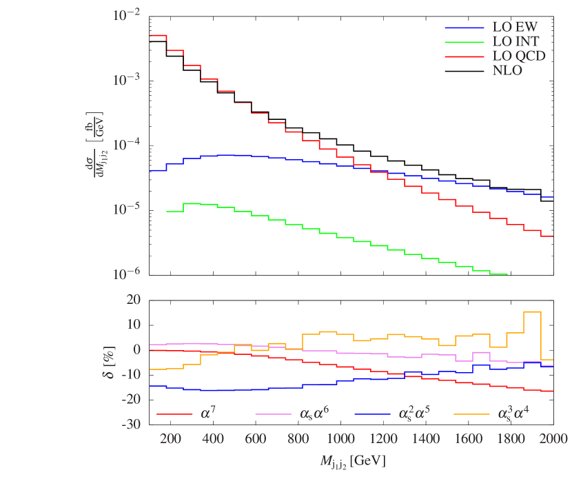
(a)

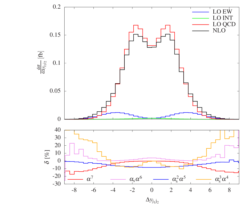
(b)

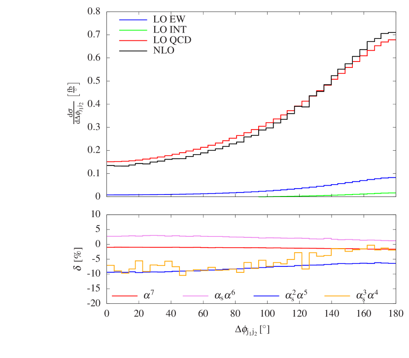
(c)

(d)

Figure 4: Separate contributions of LO and NLO. The upper panels show absolute predictions of orders $\mathcal{O}{\left(\alpha^{6}\right)}$ (LO EW), $\mathcal{O}{\left(\alpha_{\text{s}}\alpha^{5}\right)}$ (LO INT), $\mathcal{O}{\left(\alpha_{\text{s}}^{2}\alpha^{4}\right)}$ (LO QCD) and the complete NLO prediction. The lower panels display the contributions of orders $\mathcal{O}{\left(\alpha^{7}\right)}$, $\mathcal{O}{\left(\alpha_{\text{s}}\alpha^{6}\right)}$, $\mathcal{O}{\left(\alpha_{\text{s}}^{2}\alpha^{5}\right)}$, and $\mathcal{O}{\left(\alpha_{\text{s}}^{3}\alpha^{4}\right)}$ relative to the complete LO predictions. The observables read as follows: invariant mass of the two tagging jets (top left), rapidity separation of the two tagging jets (top right), azimuthal angle between the two tagging jets (bottom left), and cosine of the angle between the two tagging jets (bottom right).

The distributions in the invariant mass (Fig. 4(a)) and the rapidity separation (Fig. 4(b)) of the two tagging jets are typically used to improve the ratio of the EW component over the QCD one. These two distributions differ substantially from all others shown in this paper, since they receive sizeable contributions from the order $\mathcal{O}{\left(\alpha^{6}\right)}$ for large $M_{\text{j}_{1}\text{j}_{2}}$ or large $\Delta y_{\text{j}_{1}\text{j}_{2}}$, as can be seen in the upper part of both plots, while all other distributions are dominated by the order $\mathcal{O}{\left(\alpha_{\text{s}}^{2}\alpha^{4}\right)}$ throughout. Thus, the normalisation of the relative corrections is dominated by the $\mathcal{O}{\left(\alpha_{\text{s}}^{2}\alpha^{4}\right)}$ contributions for small $M_{\text{j}_{1}\text{j}_{2}}$ and $\Delta y_{\text{j}_{1}\text{j}_{2}}$, but by the $\mathcal{O}{\left(\alpha^{6}\right)}$ ones for large variables. Owing to this varying normalisation, the EW corrections of order $\mathcal{O}{\left(\alpha^{7}\right)}$ are large for large $M_{\text{j}_{1}\text{j}_{2}}$ or large $\Delta y_{\text{j}_{1}\text{j}_{2}}$ (reaching $-18\%$ at $M_{\text{j}_{1}\text{j}_{2}}=2\,\text{TeV}$) and small otherwise. The normalisation also explains the opposite behaviour of the (EW) corrections of order $\mathcal{O}{\left(\alpha_{\text{s}}^{2}\alpha^{5}\right)}$, which reach about $-15\%$ at $M_{\text{j}_{1}\text{j}_{2}}=400\,\text{GeV}$ but are reduced to about $-5\%$ to $-7\%$ at $2\,\text{TeV}$ in the invariant-mass distribution. Despite the fact that these large EW corrections can be traced back to Sudakov logarithms, they become relatively smaller at high energies as the LO contribution of order $\mathcal{O}{\left(\alpha_{\text{s}}^{2}\alpha^{4}\right)}$ (to which these corrections act on) is suppressed there. The corrections of QCD type, $\mathcal{O}{\left(\alpha_{\text{s}}\alpha^{6}\right)}$ and $\mathcal{O}{\left(\alpha_{\text{s}}^{3}\alpha^{4}\right)}$, stay within $\pm 10\%$ apart from the region of large rapidity separations. In particular, the QCD corrections of order $\mathcal{O}(\alpha_{\text{s}}^{3}\alpha^{4})$ turn very large (over $+40\%$) there, but this part of the phase space is rather suppressed. These QCD corrections are positive for invariant masses above $M_{\text{j}_{1}\text{j}_{2}}=500\,\text{GeV}$ and tend to increase towards higher invariant masses.

The corrections to the distributions in the azimuthal angle (Fig. 4(c)) and the cosine of the angle between the two tagging jets (Fig. 4(d)) show rather mild variations that do not exceed $10\%$ over the full phase-space range. The EW corrections of order $\mathcal{O}(\alpha^{7})$ vary by less than $2\%$ with the exception of $\cos\theta_{\text{j}_{1}\text{j}_{2}}\approx-1$. The EW corrections of order $\mathcal{O}(\alpha_{\text{s}}^{2}\alpha^{5})$ are almost $-10\%$ for small angles between the jets, while they decrease in magnitude to $-5\%$ for large angles. The pure QCD corrections of order $\mathcal{O}(\alpha_{\text{s}}^{3}\alpha^{4})$ grow in the azimuthal-angle distribution from $-10\%$ up to almost $0\%$, while they are minimal for small values of $\cos\theta_{\text{j}_{1}\text{j}_{2}}$ and maximal for $\cos\theta_{\text{j}_{1}\text{j}_{2}}=\pm 1$.

In Fig. 5, several leptonic observables are shown, including distributions in the invariant mass (Fig. 5(a)) and transverse momentum (Fig. 5(b)) of the four leptons as well as in the invariant mass (Fig. 5(c)) and the transverse momentum (Fig. 5(d)) of the electron–positron pair.

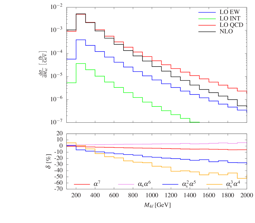
(a)

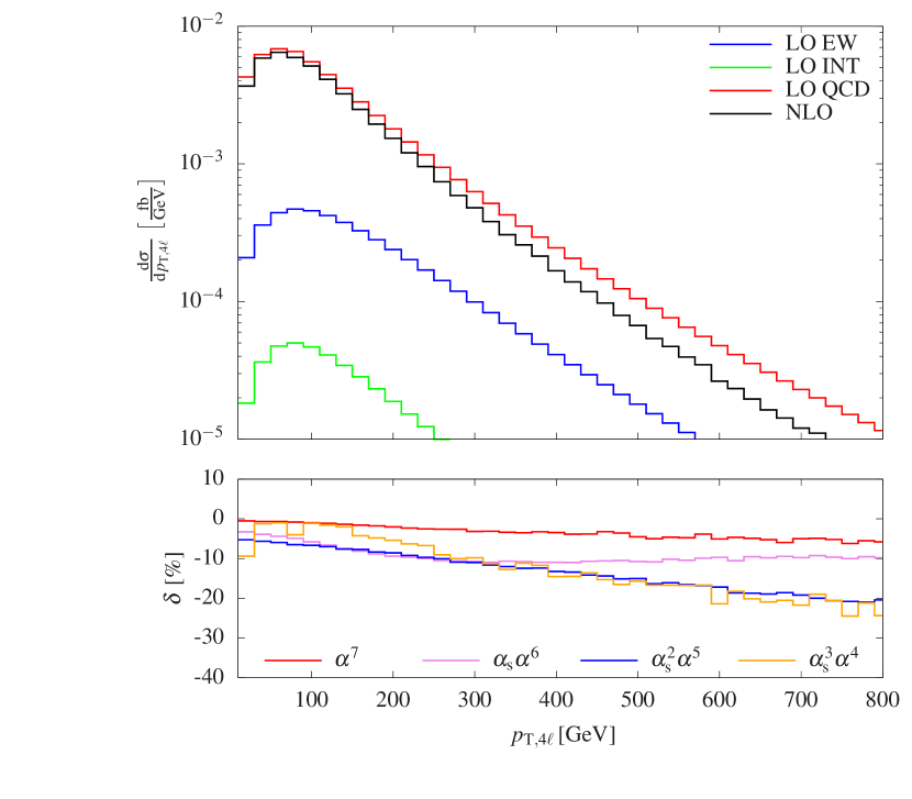
(b)

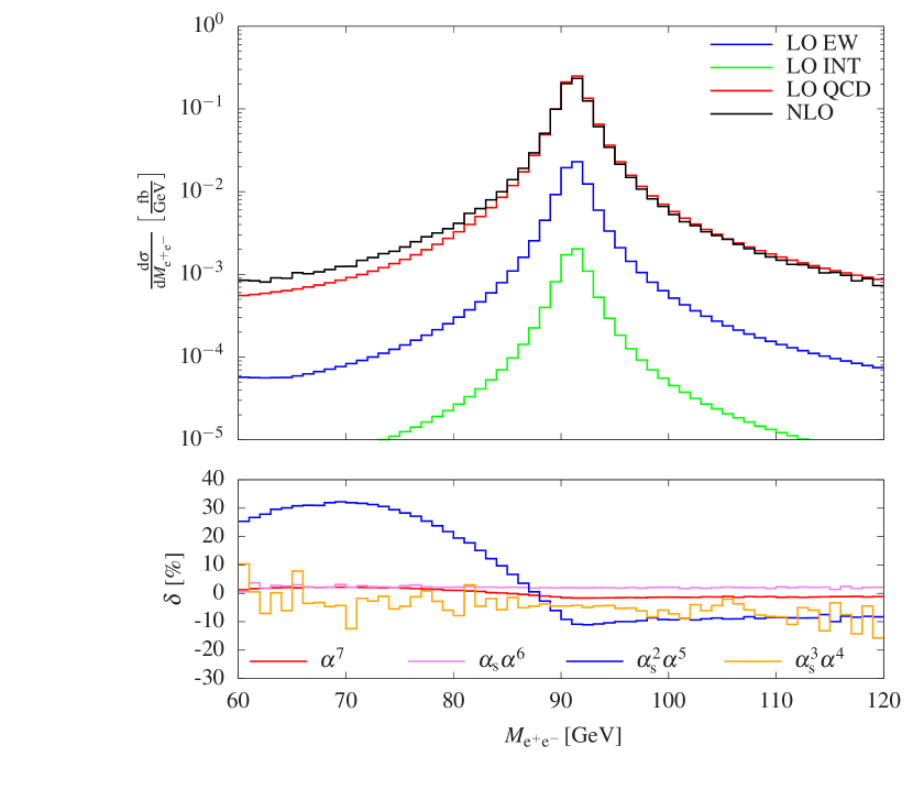
(c)

(d)

Figure 5: Same as for Fig. 4 but for the observables: invariant mass of four-lepton system (top left), transverse momentum of the four leptons (top right), invariant mass of the electron–positron system (bottom left), and transverse momentum of the electron–positron system (bottom right).

The distributions in the invariant mass and transverse momentum of the four leptons and the transverse momentum of the electron–positron pair display qualitatively rather similar features as they are correlated. In absolute, they all reach a maximum at low values to decrease steeply towards high energy. The $\mathcal{O}(\alpha_{\text{s}}^{2}\alpha^{5})$ corrections show the typical negative increase owing to Sudakov logarithms reaching up to $-30\%$ in the considered kinematical range. The corresponding behaviour of the $\mathcal{O}(\alpha^{7})$ corrections is damped by the normalisation to LO including the dominating QCD contributions. The QCD corrections of order $\mathcal{O}(\alpha_{\text{s}}^{3}\alpha^{4})$ show an even stronger impact towards high energy scales reaching $-50\%$ at $M_{4\ell}=2\,\text{TeV}$ and $-40\%$ at $p_{{\mathrm{T}},\text{e}^{+}\text{e}^{-}}=700\,\text{GeV}$. This is caused by our choice of the renormalisation scale (7) that is adapted to the VBS contributions of order $\mathcal{O}(\alpha^{6})$. For large energy scales in leptonic variables this scale is too small leading to a too large LO cross section and thus large negative QCD corrections. Note that the $\mathcal{O}(\alpha_{\text{s}}\alpha^{6})$ corrections, i.e. the QCD corrections to the VBS contributions, stay within $\pm 10\%$ for all distributions in Fig. 5. The distribution in the invariant mass of the electron–positron pair (Fig. 5(c)) is characterised by the Z-boson resonance at $\sim 91\,\text{GeV}$ in all LO contributions. While the QCD corrections are rather flat across the resonance, the EW corrections of order $\mathcal{O}(\alpha_{\text{s}}^{2}\alpha^{5})$ exhibit a pronounced radiative tail below the resonance. The corrections due to final-state photon radiation exceed $+30\%$ around $70\,\text{GeV}$. The corresponding radiative tail is also present in the corrections of order $\mathcal{O}(\alpha^{7})$ but suppressed by one order of magnitude by the LO QCD contributions.

In Fig. 6 we present distributions related to the leading jet or a single lepton.

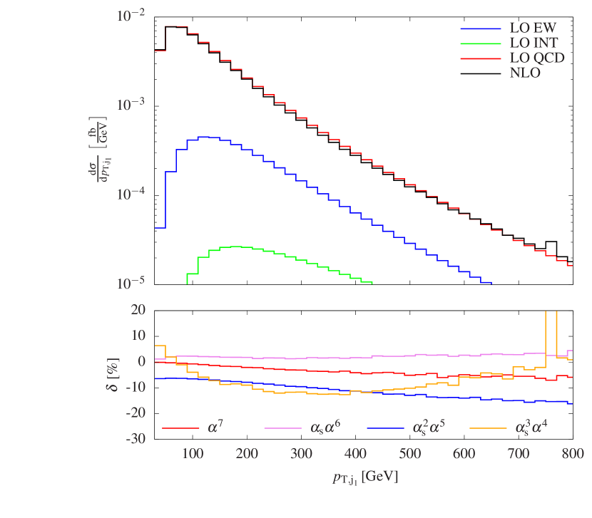
(a)

(b)

(c)

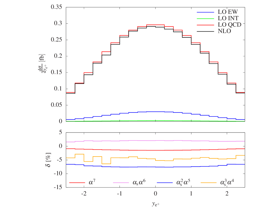
(d)

Figure 6: Same as for Fig. 4 but for the observables: transverse momentum of the hardest jet (top left), rapidity of the hardest jet (top right), transverse momentum of the muon (bottom left), and rapidity of the positron (bottom right).

In the distribution in the transverse momentum of the hardest jet (Fig. 6(a)), the corrections of order $\mathcal{O}(\alpha_{\text{s}}^{3}\alpha^{4})$ show the most interesting behaviour. They start around $6\%$ at $30\,\text{GeV}$, reach a minimum of about $-12\%$ around $350\,\text{GeV}$ to finally grow to $1\%$ at $800\,\text{GeV}$. The moderate rise of these corrections towards high transverse momenta can be attributed to the choice 7 of renormalisation scale. The increase of the QCD corrections towards small $p_{{\mathrm{T}},\text{j}_{1}}$ has already been observed in other VBS/VBF processes Biedermann:2017bss ; Denner:2019tmn ; Denner:2020zit ; Dreyer:2020xaj and is due to the real QCD radiation. The corrections of order $\mathcal{O}(\alpha_{\text{s}}^{2}\alpha^{5})$ decrease steadily towards high energy by about $10\%$. Regarding the rapidity distribution of the hardest jet (Fig. 6(b)), the corrections of order $\mathcal{O}(\alpha_{\text{s}}^{2}\alpha^{5})$ vary only by few per cent in the whole kinematic range. The $\mathcal{O}(\alpha_{\text{s}}^{3}\alpha^{4})$ corrections, on the other hand, go from $+8\%$ in the peripheral region down to $-7\%$ in the central one. The differential distributions in the transverse momentum of the muon (Fig. 6(c)) and the rapidity of the positron (Fig. 6(d)) are rather standard. The $p_{{\mathrm{T}},\mu^{-}}$ distribution behaves like other transverse-momentum distributions of leptons shown above, while the variation of all corrections to the $y_{\text{e}^{+}}$ distribution is below about two per cent.

Next we consider leptonic angular distributions in Fig. 7.

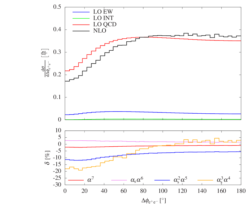
(a)

(b)

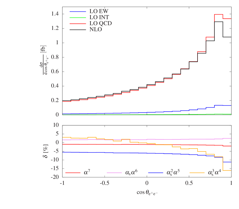
(c)

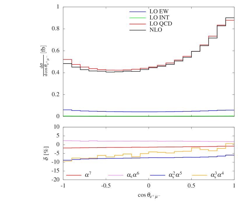
(d)

Figure 7: Same as for Fig. 4 but for the observables: azimuthal angle between the positron and the electron (top left), azimuthal angle between the positron and the muon (top right), cosine of the angle between the positron and the electron (bottom left), and cosine of the angle between the positron and the muon (bottom right).

The fraction of the LO EW contribution is somewhat enhanced for small and moderate $\cos\theta_{\text{e}^{+}\mu^{-}}$. In all distributions of Fig. 7, the corrections of orders $\mathcal{O}(\alpha^{7})$ and $\mathcal{O}(\alpha_{\text{s}}\alpha^{6})$ are small, inheriting their value from the one of the fiducial cross section. The distortion of the LO distributions results mostly from the $\mathcal{O}(\alpha_{\text{s}}^{3}\alpha^{4})$ corrections and to some extent from the $\mathcal{O}(\alpha_{\text{s}}^{2}\alpha^{5})$ corrections. Both types of corrections are largest for small angles between the electron–positron pairs and large angles between the muon–positron pairs, which typically appear for events at large energies. Thus, the variation of these corrections is driven by EW Sudakov logarithms and the choice of the QCD renormalisation scale. The corrections of order $\mathcal{O}(\alpha_{\text{s}}^{3}\alpha^{4})$ vary between $-20\%$ and $+3\%$ for different angles between electron–positron pairs and between $-10\%$ and $+3\%$ with angles between muon–positron pairs. The corresponding variations of the $\mathcal{O}(\alpha_{\text{s}}^{2}\alpha^{5})$ corrections are from $-12\%$ to $-5\%$ and from $-9\%$ to $-6\%$, respectively.

We now turn to the discussion of scale uncertainties for distributions. In the upper part of Figs. 8 and 9, absolute LO and NLO predictions are presented including 7-point variations of the QCD renormalisation and factorisation scales.

(a)

(b)

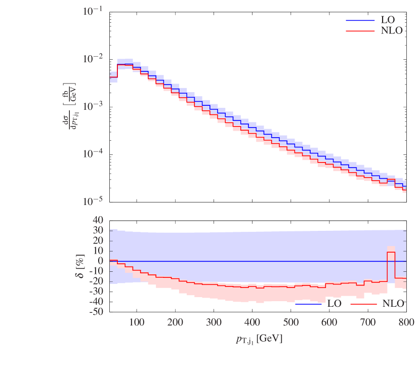
(c)

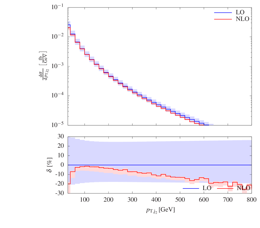
(d)

Figure 8: Differential distributions including 7-point scale uncertainties. The upper panels show absolute predictions for LO and NLO while the lower ones show relative NLO corrections with respect to the LO predictions at the central scale and the relative LO scale uncertainty. The full LO predictions include orders $\mathcal{O}(\alpha^{6})$, $\mathcal{O}(\alpha_{\text{s}}\alpha^{5})$, and $\mathcal{O}(\alpha_{\text{s}}^{2}\alpha^{4})$, while the NLO ones comprise $\mathcal{O}(\alpha^{7})$, $\mathcal{O}(\alpha_{\text{s}}\alpha^{6})$, $\mathcal{O}(\alpha_{\text{s}}^{2}\alpha^{5})$, and $\mathcal{O}(\alpha_{\text{s}}^{3}\alpha^{4})$ contributions. The observables read as follows: invariant mass of the two tagging jets (top left), rapidity difference between the two tagging jets (top right), transverse momentum of the hardest jet (bottom left), and transverse momentum of the second hardest jet (bottom right).

The lower parts show NLO corrections including scale uncertainties relative to the LO predictions at the central scale (7) together with the relative LO scale uncertainty. While the full LO predictions include the orders $\mathcal{O}(\alpha^{6})$, $\mathcal{O}(\alpha_{\text{s}}\alpha^{5})$, and $\mathcal{O}(\alpha_{\text{s}}^{2}\alpha^{4})$, the NLO ones comprise $\mathcal{O}(\alpha^{7})$, $\mathcal{O}(\alpha_{\text{s}}\alpha^{6})$, $\mathcal{O}(\alpha_{\text{s}}^{2}\alpha^{5})$, and $\mathcal{O}(\alpha_{\text{s}}^{3}\alpha^{4})$ contributions. In particular, these predictions do not include loop-induced contributions of order $\mathcal{O}{\left(\alpha_{\text{s}}^{4}\alpha^{4}\right)}$ which have already been shown in Ref. Denner:2020zit .

The total corrections to the distribution in the invariant mass of the two tagging jets (Fig. 8(a)) vary between $-10\%$ and $-30\%$ and are smallest at about $800\,\text{GeV}$. These corrections are not dominated by one particular contribution but result from the interplay of the four NLO contributions (see Fig. 4(a)). The scale uncertainty is roughly of the same size as for the fiducial cross section. On the other hand, the corrections to the distribution in the rapidity difference of the two tagging jets (Fig. 8(b)) are mostly determined by the corrections of order $\mathcal{O}(\alpha_{\text{s}}^{3}\alpha^{4})$ and to some extent of order $\mathcal{O}(\alpha_{\text{s}}^{2}\alpha^{5})$. Accidentally, the other NLO corrections cancel each other quite well. The NLO scale uncertainty strongly increases for extreme rapidity difference. The NLO corrections to the distribution in the transverse momentum of the hardest jet (Fig. 8(c)) range between $0\%$ and $-25\%$, where the overall behaviour is directed by the one of the $\mathcal{O}(\alpha_{\text{s}}^{3}\alpha^{4})$ corrections. It is worth noting that the NLO prediction is beyond the edge of the LO scale-uncertainty band for $p_{{\mathrm{T}},\text{j}_{1}}>200\,\text{GeV}$ and that the scale uncertainty for this distribution is rather large. As for all other distributions, the central value is close to the upper edge of the scale envelope. The behaviour of the NLO corrections to the distribution in the transverse momentum of the second hardest jet (Fig. 8(d)) is quite different from the one of the hardest jet. The NLO corrections are at the level of $-20\%$ at $30\,\text{GeV}$ and reach a minimum at $100\,\text{GeV}$ close to $0\%$ to steadily decrease to $-20\%$ at $800\,\text{GeV}$. The NLO scale uncertainty stays small over the whole considered kinematic range.

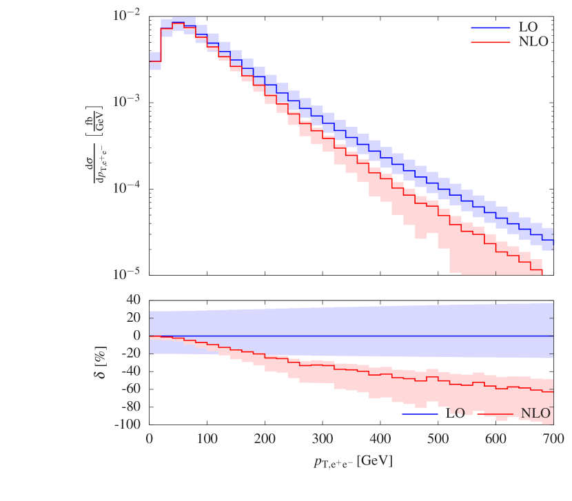
(a)

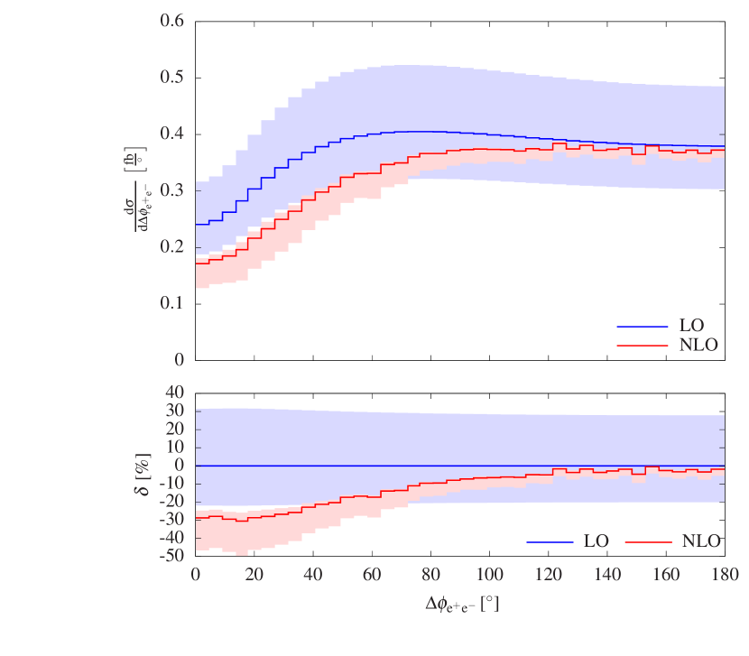
(b)

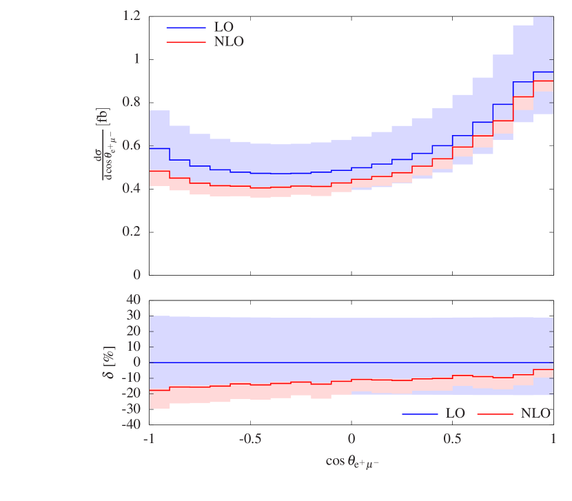
(c)

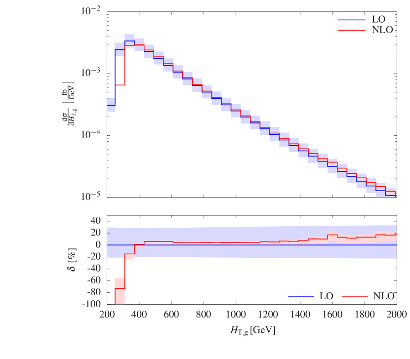
(d)

Figure 9: Same as for Fig. 8 but for the observables: transverse momentum of the electron–positron system (top left), azimuthal angle between the positron and the muon (top right), cosine of the angle between the positron and the muon (bottom left), and total transverse energy $H_{\rm T}$ (bottom right).

The NLO corrections to the distribution in the transverse momentum of the electron–positron pair, i.e. of one of the Z bosons, are shown in Fig. 9(a). As expected from Fig. 5(d), the full NLO corrections become negatively large towards high energy to reach $-60\%$ at $700\,\text{GeV}$. The NLO corrections leave the LO scale uncertainty band at about $200\,\text{GeV}$, and the NLO scale uncertainty increases significantly for high transverse momenta. This behaviour results from our scale choice (7), which is tailored to the $\mathcal{O}{\left(\alpha^{6}\right)}$ contributions but not to the dominating $\mathcal{O}{\left(\alpha_{\text{s}}^{2}\alpha^{4}\right)}$ contributions at high leptonic energies, where the scales are underestimated. The azimuthal angle between electron and positron is correlated to the transverse momentum of the electron–positron pair. Accordingly, the corrections are small for $\Delta\phi_{\text{e}^{+}\text{e}^{-}}\approx 180^{\circ}$ and increase smoothly to $-30\%$ for small $\Delta\phi_{\text{e}^{+}\text{e}^{-}}$, where the corresponding rate is minimal and the scale uncertainty is about $20\%$. Since the correlation of the angle between the positron and the muon to the transverse momentum of the electron–positron pair is smaller, the corrections vary only from $-5\%$ to $-20\%$ with increasing angle. Finally, we show the distribution in the total transverse energy, defined as the sum of transverse energies of the tagged final-state objects,

$$H_{\mathrm{T}}=E_{{\mathrm{T}},\text{e}^{+}}+E_{{\mathrm{T}},\text{e}^{-}}+E_{{\mathrm{T}},\mu^{+}}+E_{{\mathrm{T}},\mu^{-}}+E_{{\mathrm{T}},\text{j}_{1}}+E_{{\mathrm{T}},\text{j}_{2}},$$ (22)

which are defined from the transverse momenta $p_{{\mathrm{T}},i}$ as

$$E_{{\mathrm{T}},i}=\sqrt{p_{{\mathrm{T}},i}^{2}+M_{i}^{2}},$$ (23)

where the invariant mass $M_{i}$ is nonzero after recombination. The large negative corrections below $400\,\text{GeV}$ result exclusively from the order $\mathcal{O}{\left(\alpha_{\text{s}}^{3}\alpha^{4}\right)}$ corrections, more precisely from a suppression of the corresponding real contributions resulting from the restriction of the related phase space for small $H_{\mathrm{T}}$. The smooth increase of the corrections to $20\%$ at $2\,\text{TeV}$ is basically driven by the positive $\mathcal{O}{\left(\alpha_{\text{s}}^{3}\alpha^{4}\right)}$ corrections combined with negative $\mathcal{O}{\left(\alpha_{\text{s}}^{2}\alpha^{5}\right)}$ corrections. The scale uncertainty remains small apart from the region of very small $H_{\mathrm{T}}$.

4 Conclusion

Given the current and upcoming expected precision of the LHC experiments, VBS processes offer great opportunities to further probe the EW sector of the Standard Model. In this context, precision does not only refer to the EW signal that contains VBS contributions but also to the irreducible background that can be overwhelming. In addition of being sometimes large, the background can not be trivially separated from the signal making it a crucial component of any VBS studies. This calls for a full NLO description of VBS signatures including all possible contributions.

In this article we have followed this avenue by presenting full NLO predictions for $\text{p}\text{p}\to\text{e}^{+}\text{e}^{-}\mu^{+}\mu^{-}\text{j}\text{j}+X$. While some of the NLO contributions were already known in the literature, they are shown together in a unique setup for the first time here. This allows to single out salient features of VBS into ZZ pairs. It is worth noting that the hierarchy of NLO corrections is rather different from the one in the ss-WW case (which was the only channel known at full NLO accuracy up to now), in particular, owing to the appearance of partonic channels with gluons. Comparing two different setups, with different invariant-mass cuts on the two tagging jets, we have demonstrated that the LO hierarchy strongly influences the size of the NLO corrections. The newly computed corrections of order $\mathcal{O}{\left(\alpha_{\text{s}}^{2}\alpha^{5}\right)}$ turn out to be much more sizeable here than for the ss-WW signature. While for the ss-WW cross section, they were found to be below a per cent, they are between $-6\%$ and $-8\%$ (depending on the setup) for the ZZ case discussed here. We have traced back these corrections to typical EW Sudakov logarithms which appear for both signatures. While these corrections contribute for VBS into ZZ with their natural order of magnitude, they were accidentally compensated for ss-WW by QCD corrections to the LO interference appearing at the same order. This cancellation does not happen here due to the larger LO QCD contribution upon which these EW corrections act. This has an important implication: in arbitrary experimental setups, none of the four NLO corrections can safely be neglected at the $10\%$ level. Indeed, the impact of the various NLO corrections strongly depends on the hierarchy between the LO contributions which eventually originates from the experimental event selections.

In high-energy tails of distributions, the $\mathcal{O}{\left(\alpha_{\text{s}}^{2}\alpha^{5}\right)}$ corrections reach $30\%$, while the $\mathcal{O}{\left(\alpha_{\text{s}}^{3}\alpha^{4}\right)}$ corrections can amount to $50\%$. Angular distributions are distorted by up to $10\%$ and $25\%$ by the corrections of orders $\mathcal{O}{\left(\alpha_{\text{s}}^{2}\alpha^{5}\right)}$ and $\mathcal{O}{\left(\alpha_{\text{s}}^{3}\alpha^{4}\right)}$, respectively. Owing to the enhancement from Sudakov logarithms and the scale choice adapted to the VBS contributions, the total NLO corrections exceed the LO scale uncertainty band in various regions of phase space.

The results presented here should prove particularly useful for current and upcoming analyses for ZZ production in association with two jets at the LHC. We hope that experimental collaborations will take into account such NLO corrections, paving the way to precise comparisons between experimental measurements and theoretical predictions. We would like to emphasise that tailored corrections can be provided upon request.

References

- (1) R. Covarelli, M. Pellen, and M. Zaro, Vector-Boson scattering at the LHC: Unraveling the electroweak sector, Int. J. Mod. Phys. A 36 (2021) 2130009, [arXiv:2102.10991].
- (2) D. B. Franzosi et al., Vector Boson Scattering Processes: Status and Prospects, arXiv:2106.01393.
- (3) B. Biedermann, A. Denner, and M. Pellen, Large electroweak corrections to vector-boson scattering at the Large Hadron Collider, Phys. Rev. Lett. 118 (2017) 261801, [arXiv:1611.02951].
- (4) B. Biedermann, A. Denner, and M. Pellen, Complete NLO corrections to W+W+ scattering and its irreducible background at the LHC, JHEP 10 (2017) 124, [arXiv:1708.00268].
- (5) A. Denner, S. Dittmaier, P. Maierhöfer, M. Pellen, and C. Schwan, QCD and electroweak corrections to WZ scattering at the LHC, JHEP 06 (2019) 067, [arXiv:1904.00882].
- (6) A. Denner, R. Franken, M. Pellen, and T. Schmidt, NLO QCD and EW corrections to vector-boson scattering into ZZ at the LHC, JHEP 11 (2020) 110, [arXiv:2009.00411].
- (7) A. Ballestrero et al., Precise predictions for same-sign W-boson scattering at the LHC, Eur. Phys. J. C78 (2018) 671, [arXiv:1803.07943].
- (8) B. Jäger, C. Oleari, and D. Zeppenfeld, Next-to-leading order QCD corrections to Z boson pair production via vector-boson fusion, Phys. Rev. D 73 (2006) 113006, [hep-ph/0604200].
- (9) S. Alioli, P. Nason, C. Oleari, and E. Re, A general framework for implementing NLO calculations in shower Monte Carlo programs: the POWHEG BOX, JHEP 06 (2010) 043, [arXiv:1002.2581].
- (10) B. Jäger, A. Karlberg, and G. Zanderighi, Electroweak production in the Standard Model and beyond in the POWHEG-BOX V2, JHEP 03 (2014) 141, [arXiv:1312.3252].
- (11) F. Campanario, M. Kerner, L. D. Ninh, and D. Zeppenfeld, Next-to-leading order QCD corrections to ZZ production in association with two jets, JHEP 07 (2014) 148, [arXiv:1405.3972].
- (12) J. Alwall, et al., The automated computation of tree-level and next-to-leading order differential cross sections, and their matching to parton shower simulations, JHEP 07 (2014) 079, [arXiv:1405.0301].
- (13) Sherpa Collaboration, E. Bothmann et al., Event Generation with Sherpa 2.2, SciPost Phys. 7 (2019) 034, [arXiv:1905.09127].
- (14) C. Li, et al., Loop-induced production at the LHC: An improved description by matrix-element matching, Phys. Rev. D 102 (2020) 116003, [arXiv:2006.12860].
- (15) M. Chiesa, A. Denner, J.-N. Lang, and M. Pellen, An event generator for same-sign W-boson scattering at the LHC including electroweak corrections, Eur. Phys. J. C 79 (2019) 788, [arXiv:1906.01863].
- (16) ATLAS Collaboration, G. Aad et al., Observation of electroweak production of two jets and a -boson pair with the ATLAS detector at the LHC, arXiv:2004.10612.
- (17) CMS Collaboration, A. M. Sirunyan et al., Measurement of vector boson scattering and constraints on anomalous quartic couplings from events with four leptons and two jets in proton-proton collisions at TeV, Phys. Lett. B774 (2017) 682–705, [arXiv:1708.02812].
- (18) CMS Collaboration, A. M. Sirunyan et al., Evidence for electroweak production of four charged leptons and two jets in proton-proton collisions at = 13 TeV, Phys. Lett. B812 (2021) 135992, [arXiv:2008.07013].
- (19) A. Denner, S. Dittmaier, T. Kasprzik, and A. Mück, Electroweak corrections to W+jet hadroproduction including leptonic W-boson decays, JHEP 08 (2009) 075, [arXiv:0906.1656].
- (20) A. Denner, S. Dittmaier, T. Gehrmann, and C. Kurz, Electroweak corrections to hadronic event shapes and jet production in annihilation, Nucl. Phys. B836 (2010) 37–90, [arXiv:1003.0986].
- (21) A. Denner, S. Dittmaier, T. Kasprzik, and A. Mück, Electroweak corrections to dilepton + jet production at hadron colliders, JHEP 06 (2011) 069, [arXiv:1103.0914].
- (22) A. Denner, L. Hofer, A. Scharf, and S. Uccirati, Electroweak corrections to lepton pair production in association with two hard jets at the LHC, JHEP 01 (2015) 094, [arXiv:1411.0916].
- (23) ALEPH Collaboration, D. Buskulic et al., First measurement of the quark to photon fragmentation function, Z. Phys. C69 (1996) 365–378.
- (24) F. A. Berends, R. Pittau, and R. Kleiss, All electroweak four fermion processes in electron-positron collisions, Nucl. Phys. B424 (1994) 308–342, [hep-ph/9404313].
- (25) A. Denner, S. Dittmaier, M. Roth, and D. Wackeroth, Predictions for all processes fermions , Nucl. Phys. B560 (1999) 33–65, [hep-ph/9904472].
- (26) S. Dittmaier and M. Roth, LUSIFER: A LUcid approach to six FERmion production, Nucl. Phys. B642 (2002) 307–343, [hep-ph/0206070].
- (27) S. Actis, A. Denner, L. Hofer, A. Scharf, and S. Uccirati, Recursive generation of one-loop amplitudes in the Standard Model, JHEP 04 (2013) 037, [arXiv:1211.6316].
- (28) S. Actis et al., RECOLA: REcursive Computation of One-Loop Amplitudes, Comput. Phys. Commun. 214 (2017) 140–173, [arXiv:1605.01090].
- (29) A. Denner, S. Dittmaier, and L. Hofer, Collier - A fortran-library for one-loop integrals, PoS LL2014 (2014) 071, [arXiv:1407.0087].
- (30) A. Denner, S. Dittmaier, and L. Hofer, COLLIER: a fortran-based Complex One-Loop LIbrary in Extended Regularizations, Comput. Phys. Commun. 212 (2017) 220–238, [arXiv:1604.06792].
- (31) G. ’t Hooft and M. J. G. Veltman, Scalar one loop integrals, Nucl. Phys. B153 (1979) 365–401.
- (32) W. Beenakker and A. Denner, Infrared divergent scalar box integrals with applications in the electroweak Standard Model, Nucl. Phys. B338 (1990) 349–370.
- (33) S. Dittmaier, Separation of soft and collinear singularities from one-loop N-point integrals, Nucl. Phys. B675 (2003) 447–466, [hep-ph/0308246].
- (34) A. Denner and S. Dittmaier, Scalar one-loop 4-point integrals, Nucl. Phys. B844 (2011) 199–242, [arXiv:1005.2076].
- (35) G. Passarino and M. J. G. Veltman, One-loop corrections for annihilation into in the Weinberg Model, Nucl. Phys. B160 (1979) 151.
- (36) A. Denner and S. Dittmaier, Reduction of one-loop tensor 5-point integrals, Nucl. Phys. B658 (2003) 175–202, [hep-ph/0212259].
- (37) A. Denner and S. Dittmaier, Reduction schemes for one-loop tensor integrals, Nucl. Phys. B734 (2006) 62–115, [hep-ph/0509141].
- (38) M. Pellen, Exploring the scattering of vector bosons at LHCb, Phys. Rev. D101 (2020) 013002, [arXiv:1908.06805].
- (39) B. Biedermann, et al., Automation of NLO QCD and EW corrections with Sherpa and Recola, Eur. Phys. J. C77 (2017) 492, [arXiv:1704.05783].
- (40) S. Bräuer, A. Denner, M. Pellen, M. Schönherr, and S. Schumann, Fixed-order and merged parton-shower predictions for WW and WWj production at the LHC including NLO QCD and EW corrections, JHEP 10 (2020) 159, [arXiv:2005.12128].
- (41) J. R. Andersen et al., Les Houches 2017: Physics at TeV Colliders Standard Model Working Group Report, in 10th Les Houches Workshop on Physics at TeV Colliders (PhysTeV 2017) Les Houches, France, June 5-23, 2017, 2018. arXiv:1803.07977.
- (42) S. Catani and M. H. Seymour, A general algorithm for calculating jet cross-sections in NLO QCD, Nucl. Phys. B485 (1997) 291–419, [hep-ph/9605323]. [Erratum: Nucl. Phys. B510 (1998) 503].
- (43) S. Dittmaier, A general approach to photon radiation off fermions, Nucl. Phys. B565 (2000) 69–122, [hep-ph/9904440].
- (44) S. Dittmaier, A. Kabelschacht, and T. Kasprzik, Polarized QED splittings of massive fermions and dipole subtraction for non-collinear-safe observables, Nucl. Phys. B800 (2008) 146–189, [arXiv:0802.1405].
- (45) Z. Nagy and Z. Trocsanyi, Next-to-leading order calculation of four-jet observables in electron-positron annihilation, Phys. Rev. D59 (1999) 014020, [hep-ph/9806317]. [Erratum: Phys. Rev. D62 (2000) 099902].
- (46) A. Denner, S. Dittmaier, M. Roth, and L. H. Wieders, Electroweak corrections to charged-current 4 fermion processes: Technical details and further results, Nucl. Phys. B724 (2005) 247–294, [hep-ph/0505042]. [Erratum: Nucl. Phys. B854 (2012) 504].
- (47) A. Denner and S. Dittmaier, The complex-mass scheme for perturbative calculations with unstable particles, Nucl. Phys. Proc. Suppl. 160 (2006) 22–26, [hep-ph/0605312].
- (48) A. Denner and S. Dittmaier, Electroweak Radiative Corrections for Collider Physics, Phys. Rept. 864 (2020) 1–163, [arXiv:1912.06823].
- (49) NNPDF Collaboration, R. D. Ball et al., Parton distributions for the LHC Run II, JHEP 04 (2015) 040, [arXiv:1410.8849].
- (50) NNPDF Collaboration, V. Bertone, S. Carrazza, N. P. Hartland, and J. Rojo, Illuminating the photon content of the proton within a global PDF analysis, SciPost Phys. 5 (2018) 008, [arXiv:1712.07053].
- (51) J. R. Andersen et al., Les Houches 2013: Physics at TeV Colliders: Standard Model Working Group Report, arXiv:1405.1067.
- (52) A. Buckley, et al., LHAPDF6: parton density access in the LHC precision era, Eur. Phys. J. C75 (2015) 132, [arXiv:1412.7420].
- (53) A. Denner, S. Dittmaier, M. Roth, and D. Wackeroth, Electroweak radiative corrections to 4 fermions in double pole approximation: The RACOONWW approach, Nucl. Phys. B587 (2000) 67–117, [hep-ph/0006307].
- (54) Particle Data Group Collaboration, P. A. Zyla et al., Review of Particle Physics, PTEP 2020 (2020) 083C01.
- (55) D. Yu. Bardin, A. Leike, T. Riemann, and M. Sachwitz, Energy-dependent width effects in -annihilation near the Z-boson pole, Phys. Lett. B206 (1988) 539–542.
- (56) M. Cacciari, G. P. Salam, and G. Soyez, The anti- jet clustering algorithm, JHEP 04 (2008) 063, [arXiv:0802.1189].
- (57) A. Denner and S. Pozzorini, One loop leading logarithms in electroweak radiative corrections. 1. Results, Eur. Phys. J. C18 (2001) 461–480, [hep-ph/0010201].
- (58) F. A. Dreyer, A. Karlberg, J.-N. Lang, and M. Pellen, Precise predictions for double-Higgs production via vector-boson fusion, Eur. Phys. J. C 80 (2020) 1037, [arXiv:2005.13341].