Multilevel Contours on Bundles of Complex Planes

Abstract.

A new concept called multilevel contours is introduced through this article by the author. Theorems on contours constructed on a bundle of complex planes are stated and proved. Multilevel contours can transport information from one complex plane to another. Within a random environment, the behavior of contours and multilevel contours passing through the bundles of complex planes are studied. Further properties of contours by a removal process of the data are studied. The concept of ’islands’ and ’holes’ within a bundle is introduced through this article. These all constructions help to understand the dynamics of the set of points of the bundle. Further research on the topics introduced here will be followed up by the author. These include closed approximations of the multilevel contour formations and their removal processes. The ideas and results presented in this article are novel.

1. Introduction

Let us consider a bundle of eight complex planes $\mathbb{C}_{1},$ $\mathbb{C}_{2}$, $\mathbb{C}_{3}$, $\mathbb{C}_{4}$, $\mathbb{C}_{5}$, $\mathbb{C}_{6}$, $\mathbb{C}_{7}$, and $\mathbb{C}_{8}$ as shown in Figure 2.1. These planes are considered such that one plane is parallel to any other plane in the bundle or they could intersect with each other at some angle. Let $\gamma_{1}$ be an arc constructed from the points generated by $z(t_{1})\in\mathbb{\mathbb{C}}_{1}$ for $a_{11}\leq t_{1}\leq b_{11}$ such that $z(a_{11})=z_{1}$ and $z(b_{11})=z_{2}.$ Here $a_{11}$, $b_{11}\mathbb{\in R}.$ Point $z_{2}$ is located at the intersection of the planes $\mathbb{C}_{1}$ and $\mathbb{C}_{2}$. We allow constructing an arc in the plane $\mathbb{C}_{2}$ from $z_{2}$ to $z_{3}$ for $z_{3}\in\mathbb{C}_{2}$, $\mathbb{C}_{3}$, and $\mathbb{C}_{6}$. Let $\gamma_{2}$ be an arc constructed from $z(t_{2})\in\mathbb{\mathbb{C}}_{2}$ for $a_{12}\leq t_{2}\leq b_{12}$ ($a_{12}$, $b_{12}\mathbb{\in R}.$) such that $z(a_{12})=z_{2}$ and $z(b_{12})=z_{3}.$ The arc $\gamma_{i}$ is constructed by joining $z(a_{1i})=z_{i}$ and $z(b_{1i})=z_{i+1}$ generated by the set of points $z(t_{i})\text{ for }a_{1i}\leq t_{i}\leq b_{1i}$ for $i=3,4,...,7$ and $a_{1i}$, $b_{1i}\mathbb{\in R}.$ We allow the possibility to construct an arc from an ending point of an arc in a plane to a point located in a different plane if that ending point of an arc is located at the intersection of two or more complex planes. We saw above a few points lying at the intersection of two or more planes. The other points, for example, $z_{4}\in\mathbb{C}_{3}$, $\mathbb{C}_{4}$, and $\mathbb{C}_{8}$, $z_{5}\in$ $\mathbb{C}_{4}$, and $\mathbb{C}_{8}$, $z_{6}\in\mathbb{C}_{4}$, $\mathbb{C}_{6}$, and $\mathbb{C}_{8}$, $z_{7}\in\mathbb{C}_{4}$ and $\mathbb{C}_{8}$, $z_{8}\in\mathbb{C}_{7}$ and $\mathbb{C}_{8}$.

Let us form a contour by piecewise joining of arcs $\gamma_{i}$ for $i=1,2,...,7$ and call this $M_{1}.$ Let us rename the arcs corresponding to the contour $M_{1}$ be $\gamma_{i}^{M_{1}}$ for $i=1,2,...,7.$ Two more sample contours $M_{2}$ and $M_{3}$ are constructed using the points $\{z_{1},z_{2},z_{3},z_{6},z_{5}\}$, and $\{z_{1},z_{2},z_{3},z_{6},z_{8}\}$, respectively. See Figure 2.1. Let the piecewise arcs corresponding to the contour $M_{2}$ be $\gamma_{i}^{M_{2}}$ for $i=1,2,3,4,$ and the piecewise arcs corresponding to the contour $M_{3}$ be $\gamma_{i}^{M_{3}}$ for $i=1,2,3,4.$ For the sake of visualization, we have separated a single point at the intersecting planes as two or more points in different colors a smaller oval-shaped object in Figure 2.1. Suppose a contour $M_{2}$ is constructed using a set of values $z(s_{i})$ for $a_{2i}\leq s_{i}\leq a_{2i}$ with corresponding arcs $\gamma_{i}^{M_{2}}$ for $i=1,2,3,4$, and another contour $M_{3}$ is constructed $z(u_{i})$ for $a_{3i}\leq u_{i}\leq a_{3i}$ with corresponding arcs $\gamma_{i}^{M_{3}}$ for $i=1,2,3,4$. Here $a_{2i}$, $a_{3i}$, $b_{2i}$, $b_{3i}\in\mathbb{R}.$ Let

$$t_{i}=\xi_{i}(\tau)\text{ $\left(\alpha_{1i}\leq\tau\leq\beta_{1i}\right)$}$$

for $i=1,2,...,7$ be the parametric representation for a real-valued function $\xi_{i}$ mapping $[\alpha_{1i},\beta_{1i}]$ onto $[a_{1i},b_{1i}].$ Then the length of the contour $M_{1}$, say, $L(M_{1})$ is computed through the integral

(1.1) $$L(M_{1})=\sum_{i=1}^{7}\int_{\alpha_{1i}}^{\beta_{1i}}\left|z^{{}^{\prime}}[\xi_{i}(\tau)]\right|\xi_{i}^{{}^{\prime}}(\tau)d\tau.$$

Let $s_{i}=\phi_{i}(\tau)$ $(\alpha_{2i}\leq\tau\leq\beta_{2i})$ for $i=1,2,3,4$ be the parametric representation for a real-valued function $\phi_{i}$ mapping $[\alpha_{2i},\beta_{2i}]$ onto $[a_{2i},b_{2i}]$, and $u_{i}=\psi_{i}(\tau)$ $(\alpha_{3i}\leq\tau\leq\beta_{3i})$ for $i=1,2,3,4$ be the parametric representation for a real-valued function $\psi_{i}$ mapping $[\alpha_{3i},\beta_{3i}]$ onto $[a_{3i},b_{3i}].$

Then the lengths of the contours $M_{2}$ and $M_{3}$ can be computed as

(1.2) $$L(M_{2})=\sum_{i=1}^{4}\int_{\alpha_{2i}}^{\beta_{2i}}\left|z^{{}^{\prime}}[\phi_{i}(\tau)]\right|\phi_{i}^{{}^{\prime}}(\tau)d\tau,$$

(1.3) $$L(M_{3})=\sum_{i=1}^{4}\int_{\alpha_{3i}}^{\beta_{3i}}\left|z^{{}^{\prime}}[\psi_{i}(\tau)]\right|\psi_{i}^{{}^{\prime}}(\tau)d\tau.$$

The contours $M_{1},$ $M_{2}$, $M_{3}$ are located on bundle of complex planes, which we term here as multilevel contours. One can draw several such multilevel contours on a bundle of complex planes as shown in Figure 2.1. We have considered eight complex planes and three multilevel contours as an example, but one can extend these examples to demonstrate the intersection of many more complex planes and contours passing through them. Although multilevel contours are newly introduced here in this article, the principles associated with contours on a single complex plane can be found in any standard textbooks, see for example [1, 2, 3, 4].

2. Infinitely Many Bundles of Complex Planes

Let us consider infinitely many (uncountable) complex planes parallel to each other as shown in Figure 2.2 and call this $B_{\mathbb{R}}(\mathbb{C}).$ We try to form contours passing through these bundles and understand the behavior of the contours at the intersection of other planes. A contour passing through the points (complex numbers) lying in the intersection planes are given a feature to switch a plane. The points at intersections are assumed to possess special features also behavior of those points under a random environment that we will see in this article. Before we understand other properties, let us prove a Theorem.

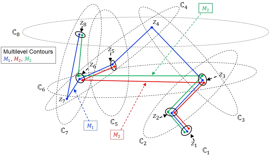
Figure 2.1. A bundle of complex planes and multilevel contours $M_{1}$, $M_{2}$, $M_{3}$.

Theorem 1.

The shortest possible multilevel contour passing through $B_{\mathbb{R}}(\mathbb{C})$ is the real line.

Proof.

Consider a complex plane that is located perpendicular to bundle $B_{\mathbb{R}}(\mathbb{C})$ such that it is at $90$ degrees with the $x-$axis. Call this $\mathbb{C}_{0}$. Using $\mathbb{C}_{0}$ we slice $B_{\mathbb{R}}(\mathbb{C})$ vertically at an arbitrary location as shown in Figure 2.2. Each slice will have uncountable lines distinct from each other, and these lines are parallel to each other. ∎

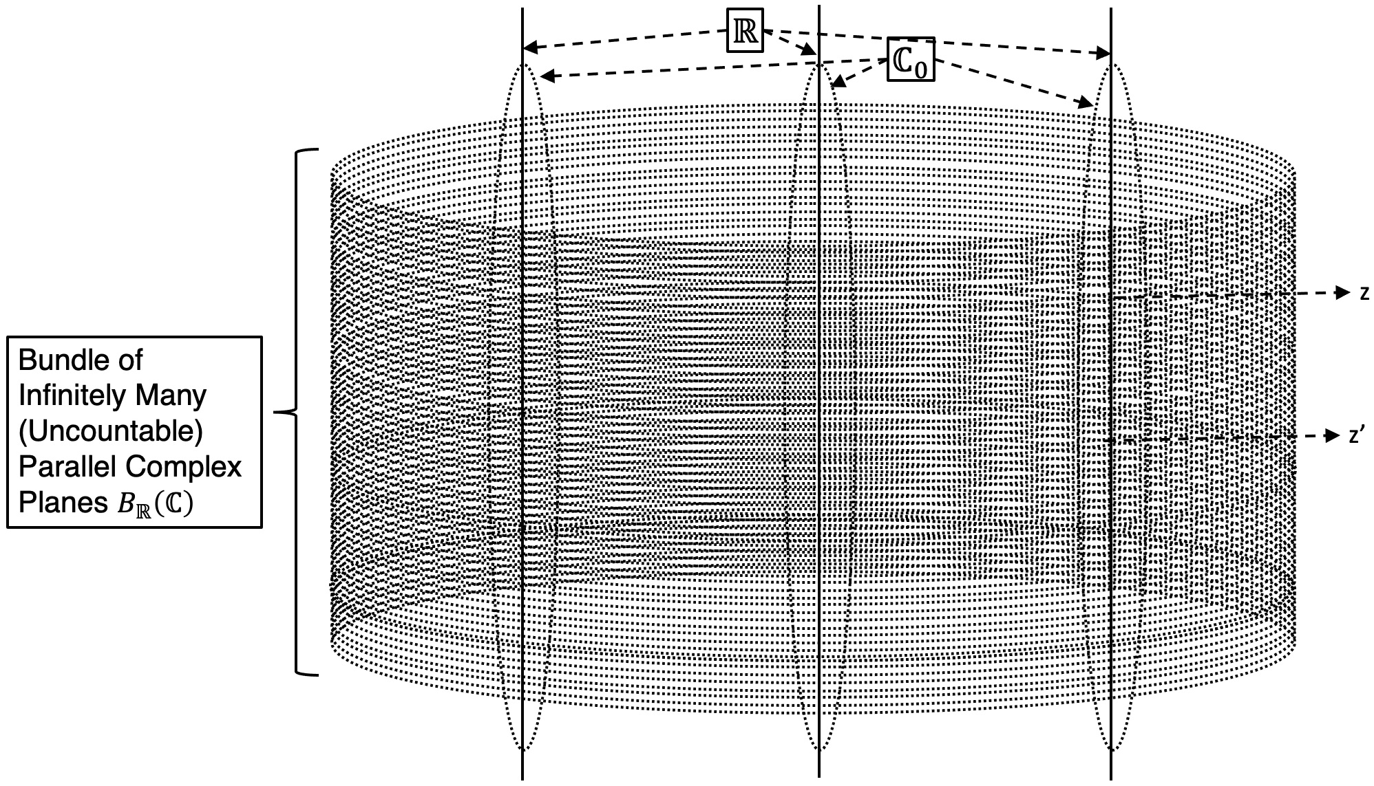
Figure 2.2. Bundle of infinitely many (uncountable) complex planes and shortest contour passing through them.

Proof.

Let $l$ and $q$ be two arbitrary lines among these uncountable lines formed out of the above slicing method. Suppose we chose a point $z_{1}$ on $l$. There exists a point $z_{2}$ on $q$ such that the $x-$coordinate and $y-$coordinate of both $z_{1}$ and $z_{2}$ are the same. Note that $z_{1},z_{2}\in\mathbb{C}_{0}$. Depending upon how we visualize the $xy-$axes of $\mathbb{C}_{0}$, the following possibilities for the values of $z_{1}$ and $z_{2}$ will arise:

(i) $z_{1}=(0,0)$ and $z_{2}=(0,0)$ or $z_{1}\neq(0,0)$ and $z_{2}\neq(0,0)$.

(ii) If $z_{1},z_{2}\neq(0,0)$, then both $z_{1}$ and $z_{2}$ will have either a non-zero $x-$coordinate (and $y-$coordinate as zero) or a non-zero $y-$coordinate (and $x-$coordinate zero). We first assume that both $z_{1}$ and $z_{2}$ are on the $y-$coordinate. Let $C(z_{1},z_{2})$ be a contour described by the equation $z(t_{1})$ for $a_{1}\leq t_{1}\leq a^{\prime}_{1},$ where $z(a_{1})=z_{1}$ for $z_{1}\in\mathbb{C}_{0},l$ and $z(a^{\prime}_{1})=z_{2}$ for $z_{2}\in\mathbb{C}_{0},q.$ Here $C(z_{1},z_{2})$ is a multilevel contour because $z_{1}$ and $z_{2}$ are points on parallel lines $l$ and $q$ on different planes but both these points also belong to $\mathbb{C}_{0}.$ Suppose

$$t_{1}=\varepsilon_{1}(\tau)\text{ $\left(\delta_{1}\leq\tau\leq\delta^{\prime}_{1}\right)$}$$

be the parametric representation for $C(z_{1},z_{2})$, where $\varepsilon_{1}$ is a real-valued function mapping $[\delta_{1},\delta^{\prime}_{1}]$ onto the interval $[a_{0},a^{\prime}_{0}].$ The length of the contour $C(z_{1},z_{2})$ is obtained by

(2.1) $$L\left[C(z_{1},z_{2})\right]=\int_{\delta_{1}}^{\delta^{\prime}_{1}}\left|z^{{}^{\prime}}[\varepsilon_{1}(\tau)]\right|\varepsilon_{1}^{{}^{\prime}}(\tau)d\tau$$

Suppose we consider a point $z_{3}$ on the same plane in which the point $z_{2}$ lies but not on the line $q$ such that $z_{3}\notin\mathbb{C}_{0}.$ That means, $z_{3}\neq z_{2}$. Let $C(z_{2},z_{3})$ be a contour described by the equation $z(t_{2})$ for $a_{2}\leq t_{2}\leq a^{\prime}_{2},$ where $z(a_{2})=z_{2}$ for $z_{2}\in\mathbb{C}_{0},q$ and $z(a^{\prime}_{2})=z_{3}$ for $z_{3}\notin\mathbb{C}_{0}\text{ and }z_{3}\notin q.$ Here $C(z_{2},z_{3})$ is not a multilevel contour. Suppose

$$t_{2}=\varepsilon_{2}(\tau)\text{ $\left(\delta_{2}\leq\tau\leq\delta^{\prime}_{2}\right)$}$$

be the parametric representation for $C(z_{2},z_{3})$, where $\varepsilon_{2}$ is a real-valued function mapping $[\delta_{2},\delta^{\prime}_{2}]$ onto the interval $[a_{2},a^{\prime}_{2}].$ The length of the contour $C(z_{2},z_{3})$ can be obtained by

(2.2) $$L\left[C(z_{2},z_{3})\right]=\int_{\delta_{2}}^{\delta^{\prime}_{2}}\left|z^{{}^{\prime}}[\varepsilon_{2}(\tau)]\right|\varepsilon_{2}^{{}^{\prime}}(\tau)d\tau.$$

Since $z_{3}$ is not in $\mathbb{C}_{0}$, we cannot draw a contour directly from $z_{1}$ to $z_{3}$. To draw a contour to $z_{3}$ from $z_{1}$, we can have piecewise arcs passing through $z_{2}$ or through any other points of the line $q$to $z_{3}.$ If the contour from $z_{1}$ to $z_{3}$ passing through $z_{2}$, then

(2.3) $$\begin{array}[]{c}\int_{\delta_{1}}^{\delta^{\prime}_{1}}\left|z^{{}^{\prime}}[\varepsilon_{1}(\tau)]\right|\varepsilon_{1}^{{}^{\prime}}(\tau)d\tau<\\ \int_{\delta_{1}}^{\delta^{\prime}_{1}}\left|z^{{}^{\prime}}[\varepsilon_{1}(\tau)]\right|\varepsilon_{1}^{{}^{\prime}}(\tau)d\tau+\int_{\delta_{2}}^{\delta^{\prime}_{2}}\left|z^{{}^{\prime}}[\varepsilon_{2}(\tau)]\right|\varepsilon_{2}^{{}^{\prime}}(\tau)d\tau,\end{array}$$

If the contour from $z_{1}$ to $z_{3}$ passing through an arbitrary point, say, $z_{4}$ $(z_{4}\neq z_{2})$ for $z_{4}\in q$, then

(2.4) $$\int_{\delta_{1}}^{\delta^{\prime}_{1}}\left|z^{{}^{\prime}}[\varepsilon_{1}(\tau)]\right|\varepsilon_{1}^{{}^{\prime}}(\tau)d\tau<\int_{\delta_{3}}^{\delta^{\prime}_{3}}\left|z^{{}^{\prime}}[\varepsilon_{3}(\tau)]\right|\varepsilon_{3}^{{}^{\prime}}(\tau)d\tau,$$

where the R.H.S. of the inequality (2.4) is the length of the contour $C(z_{1},z_{4})$ described by the equation $z(t_{3})$ for $a_{3}\leq t_{3}\leq a^{\prime}_{3},$ where $z(a_{3})=z_{1}$ for $z_{1}\in\mathbb{C}_{0},l$ and $z(a^{\prime}_{3})=z_{4}$ for $z_{4}\in\mathbb{C}_{0}.$ Here $t_{3}=\varepsilon_{3}(\tau)\text{ $\left(\delta_{3}\leq\tau\leq\delta^{\prime}_{3}\right)$}$ is the parametric representation for $C(z_{1},z_{4})$ and $\varepsilon_{3}$ is a real-valued function mapping $[\delta_{3},\delta^{\prime}_{3}]$ onto the interval $[a_{3},a^{\prime}_{3}].$ From (2.4) and (LABEL:eq), we have

$$\int_{\delta_{1}}^{\delta^{\prime}_{1}}\left|z^{{}^{\prime}}[\varepsilon_{1}(\tau)]\right|\varepsilon_{1}^{{}^{\prime}}(\tau)d\tau+\int_{\delta_{2}}^{\delta^{\prime}_{2}}\left|z^{{}^{\prime}}[\varepsilon_{2}(\tau)]\right|\varepsilon_{2}^{{}^{\prime}}(\tau)d\tau$$

(2.5) $$<\int_{\delta_{3}}^{\delta^{\prime}_{3}}\left|z^{{}^{\prime}}[\varepsilon_{3}(\tau)]\right|\varepsilon_{3}^{{}^{\prime}}(\tau)d\tau+\int_{\delta_{4}}^{\delta^{\prime}_{4}}\left|z^{{}^{\prime}}[\varepsilon_{4}(\tau)]\right|\varepsilon_{4}^{{}^{\prime}}(\tau)d\tau,$$

where the second term of R.H.S. of the inequality (2.5) is the length of the contour $C(z_{4},z_{3})$ described by the equation $z(t_{4})$ for $a_{4}\leq t_{4}\leq a^{\prime}_{4},$ where $z(a_{4})=z_{4}$ for $z_{4}\in\mathbb{C}_{0},q$ and $z(a^{\prime}_{4})=z_{3}$ for $z_{3}\neq\mathbb{C}_{0}.$ Here $t_{4}=\varepsilon_{4}(\tau)\text{ $\left(\delta_{4}\leq\tau\leq\delta^{\prime}_{4}\right)$}$ is the parametric representation for contour $C(z_{4},z_{3})$ and $\varepsilon_{4}$ is a real-valued function mapping $[\delta_{4},\delta^{\prime}_{4}]$ onto the interval $[a_{4},a^{\prime}_{4}].$ From (LABEL:eq) to (2.5) we conclude that $L\left[C(z_{1},z_{2})\right]$ is the shortest contour and it is a line. We can chose a point $z$ on a line $p$ for $p\in\mathbb{C}_{0}$ and find a corresponding point $z^{\prime}$ on a line, say, $p^{\prime}$ for $p^{\prime}\in\mathbb{C}_{0}$ and construct an argument as above to see that $L\left[C(z,z^{\prime})\right]$ is the shortest. The $x$ and $y$ coordinates of $z$ and $z^{\prime}$ are the same. We can construct infinitely many contours between various points $z$, $z^{\prime}$ lying on the slice such that $L\left[C(z,z^{\prime})\right]$ is the shortest. If $p$ and $p^{\prime}$ are the lines from adjacent planes then

(2.6) $$\bigcup_{z,z^{\prime}}\int_{\delta_{p}}^{\delta^{\prime}_{p}}\left|z^{{}^{\prime}}[\varepsilon_{p}(\tau)]\right|\varepsilon_{p}^{{}^{\prime}}(\tau)d\tau=\infty$$

and

$$\bigcup_{z,z^{\prime}}C\left(z,z^{\prime}\right)\sim\mathbb{R}.$$

In (2.6), the integral on the LH.S. is the length of the contour $C(z,z^{\prime})$ described by the equation $z(t_{p})$ for $a_{p}\leq t_{p}\leq a^{\prime}_{p},$ where $z(a_{p})=z$ for $z\in\mathbb{C}_{0},p$ and $z(a^{\prime}_{p})=z^{\prime}$ for $z^{\prime}\in p^{\prime},\mathbb{C}_{0}.$ Here $t_{p}=\varepsilon_{p}(\tau)\text{ $\left(\delta_{p}\leq\tau\leq\delta^{\prime}_{p}\right)$}$ is the parametric representation for contour $C(z,z^{\prime})$ and $\varepsilon_{p}$ is a real-valued function mapping $[\delta_{p},\delta^{\prime}_{p}]$ onto the interval $[a_{p},a^{\prime}_{p}].$ ∎

Remark 2.

Let $z_{n}$ be a sequence on the slice $\mathbb{C}_{0}$. then

$$\lim_{n\rightarrow\infty}z_{n}=z$$

since $z$ is equal to $z_{n}$ $\forall n.$

Remark 3.

Remark (2) is true for each slice on the bundle that is parallel to $\mathbb{C}.$ But the limits of convergence on each slice are different.

Remark 4.

The distances between each pair of adjacent points on every contour created by slicing parallel to $\mathbb{C}_{0}$ are equal.

Suppose we remove the space created by $\mathbb{C}_{0}$ from the bundle $B_{\mathbb{R}}(\mathbb{C})$, then the bundle formed on the left of $\mathbb{C}_{0}$ be denoted by $B_{\mathbb{R}}^{L}(\mathbb{C}_{0})$ and the bundle formed on the right of $\mathbb{C}_{0}$ be denoted by $B_{\mathbb{R}}^{R}(\mathbb{C}_{0}).$ Then

(2.7) $$B_{\mathbb{R}}^{L}(\mathbb{C}_{0})\cup\mathbb{C}_{0}\cup B_{\mathbb{R}}^{R}(\mathbb{C}_{0})=B_{\mathbb{R}}(\mathbb{C})$$

The set $B_{\mathbb{R}}(\mathbb{C})-\mathbb{C}_{0}$ is defined as

$$B_{\mathbb{R}}(\mathbb{C})-\mathbb{C}_{0}=\left\{z:z\in B_{\mathbb{R}}(\mathbb{C})\text{ and }z\notin\mathbb{C}_{0}\right\}$$

forms a disconnected set because

(2.8) $$B_{\mathbb{R}}(\mathbb{C})-\mathbb{C}_{0}=B_{\mathbb{R}}^{L}(\mathbb{C}_{0})\cup B_{\mathbb{R}}^{R}(\mathbb{C}_{0})$$

and $B_{\mathbb{R}}^{L}(\mathbb{C}_{0})$ and $B_{\mathbb{R}}^{R}(\mathbb{C}_{0})$ are disjoint and non-empty sets within $B_{\mathbb{R}}(\mathbb{C}).$ No multilevel contours can be drawn passing through various planes of the bundle $B_{\mathbb{R}}^{L}(\mathbb{C}_{0})$ unless $B_{\mathbb{R}}^{L}(\mathbb{C}_{0})$ is sliced similarly as we did for the bundle $B_{\mathbb{R}}(\mathbb{C})$. Under similar circumstances, no multilevel contours can be drawn passing through the planes of $B_{\mathbb{R}}^{R}(\mathbb{C}_{0}).$ Suppose we slice the bundle $B_{\mathbb{R}}^{L}(\mathbb{C}_{0})$ with a complex plane that was kept parallel to $\mathbb{C}_{0}$ and call this new plane $\mathbb{C}_{r}$ ($r>0$) that was used for slicing. Now $\mathbb{C}_{1}$ intersects with each and every plane of $B_{\mathbb{R}}^{L}(\mathbb{C}_{0}).$ Let us remove the space created by $\mathbb{C}_{r}$ from $B_{\mathbb{R}}^{L}(\mathbb{C}_{0})$ to form a new disjoint bundles $B_{\mathbb{R}}^{L}(\mathbb{C}_{r})$ and $B_{\mathbb{R}}^{R}(\mathbb{C}_{r})$ such that

(2.9) $$B_{\mathbb{R}}^{L}(\mathbb{C}_{r})\cup\mathbb{C}_{r}\cup B_{\mathbb{R}}^{R}(\mathbb{C}_{r})=B_{\mathbb{R}}^{L}(\mathbb{C}_{0}),$$

where $B_{\mathbb{R}}^{L}(\mathbb{C}_{r})$ is the bundle formed on the left of $\mathbb{C}_{r}$ and $B_{\mathbb{R}}^{R}(\mathbb{C}_{r})$ is the bundle formed on the right of $\mathbb{C}_{r}$ due to removal of the space $\mathbb{C}_{r}$ from $B_{\mathbb{R}}^{L}(\mathbb{C}_{0}).$ Using the similar argument of (2.8), we write below $B_{\mathbb{R}}^{L}(\mathbb{C}_{0})-\mathbb{C}_{r}$ as an union of two disconnected sets

(2.10) $$B_{\mathbb{R}}^{L}(\mathbb{C}_{0})-\mathbb{C}_{r}=B_{\mathbb{R}}^{L}(\mathbb{C}_{r})\cup B_{\mathbb{R}}^{R}(\mathbb{C}_{r})\>\text{}(r>0)$$

Although we could not draw a multilevel contour passing through all the planes of the bundle $B_{\mathbb{R}}^{L}(\mathbb{C}_{r})$, one can draw such a contour through the plane $\mathbb{C}_{r}$ while it intersects the bundle $B_{\mathbb{R}}^{L}(\mathbb{C}_{r}).$ One can write another disjoint set

(2.11) $$B_{\mathbb{R}}^{L}(\mathbb{C}_{r})-\mathbb{C}_{r^{\prime}}=B_{\mathbb{R}}^{L}(\mathbb{C}_{r^{\prime}})\cup B_{\mathbb{R}}^{R}(\mathbb{C}_{r^{\prime}})\>\text{}(r,r^{\prime}>0),$$

where $\mathbb{C}_{r^{\prime}}$ is complex plane used to slice $B_{\mathbb{R}}^{L}(\mathbb{C}_{r^{\prime}})$ and $\mathbb{C}_{r}$ is complex plane used to slice $B_{\mathbb{R}}^{L}(\mathbb{C}_{0}).$

Let us now consider right side of the plane $\mathbb{C}_{0}$ within the bundle $B_{\mathbb{R}}(\mathbb{C})$ i.e. $B_{\mathbb{R}}^{R}(\mathbb{C}_{0}).$ Suppose we slice the bundle $B_{\mathbb{R}}^{R}(\mathbb{C}_{0})$ using a plane parallel to $\mathbb{C}_{0}$ and call this $\mathbb{C}_{s}$ ($s>0)$. Let us remove the space created by $\mathbb{C}_{s}$ from $B_{\mathbb{R}}^{R}(\mathbb{C}_{0})$ such that

(2.12) $$B_{\mathbb{R}}^{R}(\mathbb{C}_{0})-\mathbb{C}_{s}=B_{\mathbb{R}}^{L}(\mathbb{C}_{s})\cup B_{\mathbb{R}}^{R}(\mathbb{C}_{r})\>\text{}(s>0).$$

From the above constructions (2.7) through (2.12), the set of points of the bundle $B_{\mathbb{R}}(\mathbb{C})$ with intersecting planes $\mathbb{C}_{r}$, $\mathbb{C}_{0}$, $\mathbb{C}_{s}$ are written as

$$B_{\mathbb{R}}(\mathbb{C}) =B_{\mathbb{R}}^{L}(\mathbb{C}_{0})\cup\mathbb{C}_{0}\cup B_{\mathbb{R}}^{R}(\mathbb{C}_{0})$$

(2.13) $$=\left[B_{\mathbb{R}}^{L}(\mathbb{C}_{r})\cup\mathbb{C}_{r}\cup B_{\mathbb{R}}^{R}(\mathbb{C}_{r})\right]\cup\mathbb{C}_{0}\cup\left[B_{\mathbb{R}}^{L}(\mathbb{C}_{s})\cup\mathbb{C}_{s}\cup B_{\mathbb{R}}^{R}(\mathbb{C}_{s})\right]$$

$\implies$

$$B_{\mathbb{R}}(\mathbb{C})-\left(\mathbb{C}_{0}\cup\mathbb{C}_{r}\cup\mathbb{C}_{r}\right) =$$

(2.14) $$\left[B_{\mathbb{R}}^{L}(\mathbb{C}_{r})\cup B_{\mathbb{R}}^{R}(\mathbb{C}_{r})\right]\cup\left[B_{\mathbb{R}}^{L}(\mathbb{C}_{s})\cup B_{\mathbb{R}}^{R}(\mathbb{C}_{s})\right]$$

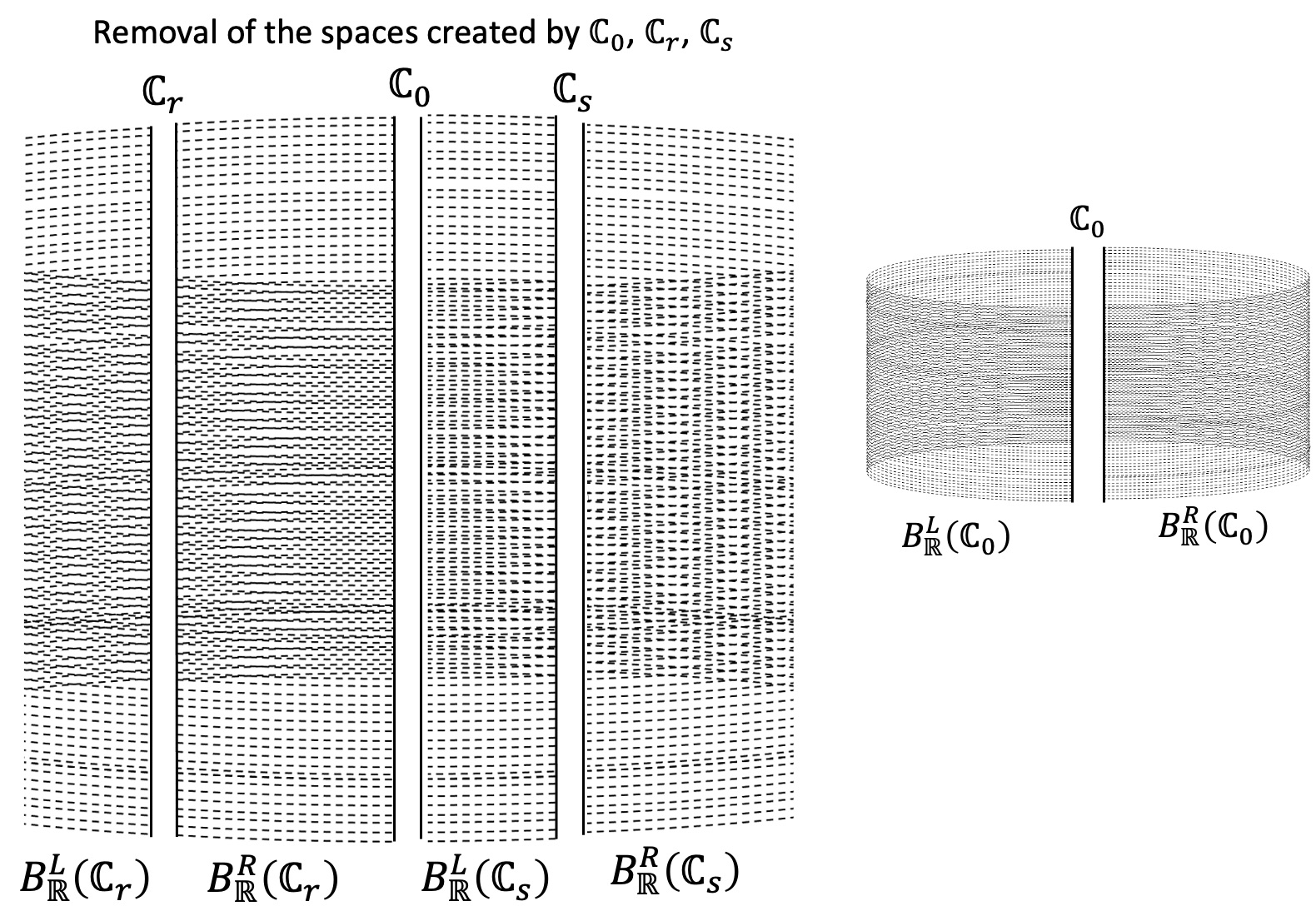
Figure 2.3. Creation of disconnected sets out of the bundle $B_{\mathbb{R}}(\mathbb{C})$ due to the slicing and removal of the spaces created by the complex planes $\mathbb{C}_{0}$, $\mathbb{C}_{r}$, $\mathbb{C}_{s}$.

The four disconnected sets in (2.14) can be used for forming infinitely many disconnected sets. Due to the removal of the spaces as shown in Figure 2.3, it is impossible to draw multilevel contours within and between these four disconnected sets in (2.14). One of the advantages of multilevel contours is to develop trees of arcs, paths that can be used for transportation of information between two or more interacting (intersecting) complex planes. The bundle B(C) have parallel planes however the contours drawn within each of these planes need not be similar. One can construct a functional mapping such that a contour or an arc drawn in one plane could be mapped to a contour or an arc in another plane. But these two sets of contours could be used for transporting information continuously only if these contours in two or more planes are path-connected (Figure 2.4).

Suppose $S_{1}$, $S_{2}$, $S_{3}$, $S_{4}$ are four contours drawn for specific purposes in four different complex planes $\mathbb{C}_{1},$ $\mathbb{C}_{2}$, $\mathbb{C}_{3}$, $\mathbb{C}_{4}$, respectively. Let $S_{i}$ be described by $z(t)$ for $a_{s_{i}}\leq t_{s_{1}}\leq a^{\prime}_{s_{i}}$ where $a_{s_{i}},$ $a^{\prime}_{s_{i}}\in\mathbb{R}$ for $i=1,2,3,4.$ See Figure 2.4. Had these four planes have no intersecting set of points, then one couldn’t construct multilevel contours passing through these planes. Let $z(a_{s_{i}})=z_{1}^{S_{i}}$ be the starting point and $z(a^{\prime}_{s_{i}})=z_{2}^{S_{i}}$ be the ending point of the contour $S_{i}$ for $i=1,2,3,4.$ Suppose each independent contour $S_{i}$ has a specific information stored in it. Information stored in $S_{1}$ is transferred to the contour $S_{2}$ using a contour $T_{1}$. Suppose $\mathbb{C}_{1}\cap\mathbb{C}_{2}=\left\{z:z\in\mathbb{C}_{1}\text{ and }z\mathbb{\in C}_{2}\right\}$. Then for the structure of the planes and contours $S_{1}$ through $S_{4}$ in Figure 2.4, we have $\mathbb{C}_{1}\cap\mathbb{C}_{2}\neq\phi$ (empty set) and $S_{1}\cap\left(\mathbb{C}_{1}\cap\mathbb{C}_{2}\right)=\phi$. Let $T_{1}$ be a contour drawn from a point in $S_{1}$ to a point in $S_{2}$ through a set of points for which $\mathbb{C}_{1}\cap\mathbb{C}_{2}\neq\phi.$ $T_{1}$ is described by $z(u_{t_{1}})$ for $a_{t_{1}}\leq u_{t_{1}}\leq a^{\prime}_{t_{1}}$ where $a_{t_{1}},$ $a^{\prime}_{t_{1}}\in\mathbb{R}$. The starting point of $T_{1}$ lies on $S_{1}$ and the ending point of $T_{1}$ lies on $S_{2}$. We call $T_{1}$ a transporting contour. Using $T_{1}$ the information stored in $S_{1}$ and $S_{2}$ can be communicated. We will discuss later more features on information transfer. The length of the multilevel contour due to $S_{1}$, $T_{1}$, $S_{2}$ , say $L[S_{1},S_{2}]$ is computed as

$$L[S_{1},S_{2}] =\int_{\delta_{s_{1}}}^{\delta^{\prime}_{s_{1}}}\left|z[\varepsilon_{s_{1}}(\tau)]\right|\varepsilon_{s_{1}}^{{}^{\prime}}(\tau)d\tau+\int_{\omega_{t_{1}}}^{\omega_{t_{1}}^{\prime}}\left|z[\eta_{t_{1}}(\tau)]\right|\eta_{t_{1}}^{{}^{\prime}}(\tau)d\tau$$

(2.15) $$+\int_{\delta_{s_{2}}}^{\delta^{\prime}_{s_{2}}}\left|z[\varepsilon_{s_{2}}(\tau)]\right|\varepsilon_{s_{2}}^{{}^{\prime}}(\tau)d\tau$$

Here $t_{s_{i}}=\varepsilon_{s_{i}}(\tau)\text{ $\left(\delta_{s_{i}}\leq\tau\leq\delta^{\prime}_{s_{i}}\right)$}$ for $i=1,2,3,4$ is the parametric representation for contour $S_{i}$ with a real-valued function $\varepsilon_{s_{i}}$ mapping $[\delta_{s_{i}},\delta^{\prime}_{s_{i}}]$ onto the interval $[a_{s_{i}},a^{\prime}_{s_{i}}],$ and $u_{t_{1}}=\eta_{t_{1}}(\tau)\text{ $\left(\omega_{t_{1}}\leq\tau\leq\omega^{\prime}_{t_{1}}\right)$}$ is the parametric representation for contour $T_{1}$ with a real-valued function $\eta_{t_{1}}$ mapping $[\omega_{t_{1}},\omega^{\prime}_{t_{1}}]$ onto the interval $[a_{t_{1}},a^{\prime}_{t_{1}}]$. Since the total information stored in $S_{1}$ and $S_{2}$ are exchanged we have considered total lengths of $S_{1}$ and $S_{2}$ even though $T_{1}$ could be connected with any point of $S_{1}$ and $S_{2}$. Since $z(a_{t_{1}})\in S_{1}$ and $z(a_{t_{2}})\in S_{2}$ and the $T_{1}$ describes a contour from $z(a_{t_{1}})$ to $z(a_{t_{2}})$, the length of the middle integral in R.H.S. of (2.15) is not constant. The transportation contour can be used to transport information from $S_{2}$ to $S_{1}$. Let us denote this by the contour $T^{\prime}_{1}$. In that case, the starting point of $T^{\prime}_{1}$ lies on $S_{2}$, and the ending point of $T^{\prime}_{1}$ lies on $S_{1}$. $T^{\prime}_{1}$ is described by $z^{\prime}(u^{\prime}_{t_{1}})$ for $a_{t_{1}}\leq u_{t_{1}}\leq a^{\prime}_{t_{1}}$ where $a_{t_{1}},$ $a^{\prime}_{t_{1}}\in\mathbb{R}$, and $u^{\prime}_{t_{1}}=\eta*_{t_{1}}(\tau)\text{ $\left(\omega_{t_{1}}\leq\tau\leq\omega^{\prime}_{t_{1}}\right)$}$ is the parametric representation for contour $T^{\prime}_{1}$ with a real-valued function $\eta*_{t_{1}}$ mapping $[\omega_{t_{1}},\omega^{\prime}_{t_{1}}]$ onto the interval $[a_{t_{1}},a^{\prime}_{t_{1}}]$. When we measure the length $S_{2}$ to $S_{1}$, sat $L(S_{2},S_{1}]$, the orientation of the transportation contour changes, and it is computed as

$$L[S_{2},S_{1}] =\int_{\delta_{s_{1}}}^{\delta^{\prime}_{s_{1}}}\left|z[\varepsilon_{s_{1}}(\tau)]\right|\varepsilon_{s_{1}}^{{}^{\prime}}(\tau)d\tau+\int_{\omega^{\prime}_{t_{1}}}^{\omega_{t_{1}}}\left|z[\eta*_{t_{1}}(\tau)]\right|\eta*_{t_{1}}^{{}^{\prime}}(\tau)d\tau$$

(2.16) $$+\int_{\delta_{s_{2}}}^{\delta^{\prime}_{s_{2}}}\left|z[\varepsilon_{s_{2}}(\tau)]\right|\varepsilon_{s_{2}}^{{}^{\prime}}(\tau)d\tau$$

The values of the middle integrals in the R.H.S. of (2.15) and (2.16) need not be the same unless the below condition is satisfied:

(2.17) $$z(a_{t_{1}}),\text{ }z^{\prime}(a^{\prime}_{t_{1}})\in S_{1}\text{ and }z^{\prime}(a_{t_{1}})\text{ }z(a^{\prime}_{t_{1}})\in S_{2}.$$

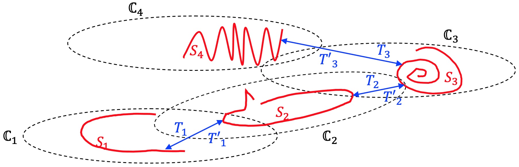
Figure 2.4. Transportation of information through multilevel contours $S_{1}$,$...,$$S_{7}$ passing through four intersecting complex planes $\mathbb{C}_{1}$, $\mathbb{C}_{2}$, $\text{$\mathbb{C}$}_{3}$, and $\mathbb{C}_{4}$.

The transportation contour $T_{2}$ joins $S_{2}$ to $S_{3}$ and the transportation contour $T^{\prime}_{2}$ joins $S_{3}$ to $S_{2}.$ The contour $T_{2}$ is described by $z(u_{t_{2}})$ for $a_{t_{2}}\leq u_{t_{2}}\leq a^{\prime}_{t_{2}}$ where $a_{t_{2}},$ $a^{\prime}_{t_{2}}\in\mathbb{R}$. The starting point of $T_{2}$ is in the set $S_{2}$ and the ending point of $T_{2}$ is in the set $S_{3}$. The function $u_{t_{2}}=\eta_{t_{2}}(\tau)\text{ $\left(\omega_{t_{2}}\leq\tau\leq\omega^{\prime}_{t_{2}}\right)$}$ is the parametric representation for contour $T_{2}$ with a real-valued function $\eta_{t_{2}}$ mapping $[\omega_{t_{2}},\omega^{\prime}_{t_{2}}]$ onto the interval $[a_{t_{2}},a^{\prime}_{t_{2}}]$. The contour $T^{\prime}_{2}$ is described by $z(u^{\prime}_{t_{2}})$ for $a_{t_{2}}\leq u^{\prime}_{t_{2}}\leq a^{\prime}_{t_{2}}$ where $a_{t_{2}},$ $a^{\prime}_{t_{2}}\in\mathbb{R}$, and the function $u^{\prime}_{t_{2}}=\eta*_{t_{2}}(\tau)\text{ $\left(\omega_{t_{2}}\leq\tau\leq\omega^{\prime}_{t_{2}}\right)$}$ is the parametric representation for contour $T^{\prime}_{2}$ with a real-valued function $\eta*_{t_{2}}$ mapping $[\omega_{t_{2}},\omega^{\prime}_{t_{2}}]$ onto the interval $[a_{t_{2}},a^{\prime}_{t_{2}}]$. The lengths of these transportation contours can be computed and

$$\int_{\omega_{t_{2}}}^{\omega_{t_{2}}^{\prime}}\left|z[\eta_{t_{2}}(\tau)]\right|\eta_{t_{2}}^{{}^{\prime}}(\tau)d\tau=\int_{\omega^{\prime}_{t_{2}}}^{\omega_{t_{2}}}\left|z[\eta*_{t_{2}}(\tau)]\right|\eta*_{t_{2}}^{{}^{\prime}}(\tau)d\tau$$

if, and only, if

$$z(a_{t_{2}}),\text{ }z^{\prime}(a^{\prime}_{t_{2}})\in S_{2}\text{ and }z^{\prime}(a_{t_{2}})\text{ }z(a^{\prime}_{t_{2}})\in S_{3}.$$

The multilevel contour lengths of $S_{2}$ to $S_{3}$ and $S_{3}$ to $S_{2}$ are computed as

$$L[S_{2},S_{3}] =\int_{\delta_{s_{2}}}^{\delta^{\prime}_{s_{2}}}\left|z[\varepsilon_{s_{2}}(\tau)]\right|\varepsilon_{s_{2}}^{{}^{\prime}}(\tau)d\tau+\int_{\omega_{t_{2}}}^{\omega_{t_{2}}^{\prime}}\left|z[\eta_{t_{2}}(\tau)]\right|\eta_{t_{2}}^{{}^{\prime}}(\tau)d\tau$$

(2.18) $$+\int_{\delta_{s_{3}}}^{\delta^{\prime}_{s_{3}}}\left|z[\varepsilon_{s_{3}}(\tau)]\right|\varepsilon_{s_{3}}^{{}^{\prime}}(\tau)d\tau$$

$$L[S_{3},S_{2}] =\int_{\delta_{s_{2}}}^{\delta^{\prime}_{s_{2}}}\left|z[\varepsilon_{s_{2}}(\tau)]\right|\varepsilon_{s_{2}}^{{}^{\prime}}(\tau)d\tau+$$

$$\int_{\omega^{\prime}_{t_{2}}}^{\omega_{t_{2}}}\left|z[\eta*_{t_{2}}(\tau)]\right|\eta*_{t_{2}}^{{}^{\prime}}(\tau)d\tau+$$

(2.19) $$\int_{\delta_{s_{3}}}^{\delta^{\prime}_{s_{3}}}\left|z[\varepsilon_{s_{3}}(\tau)]\right|\varepsilon_{s_{3}}^{{}^{\prime}}(\tau)d\tau$$

The transportation contour $T_{3}$ joins $S_{3}$ to $S_{4}$ and the return transportation contour $T^{\prime}_{3}$ joins $S_{4}$ to $S_{4}.$ The contour $T_{3}$ is described by $z(u_{t_{3}})$ for $a_{t_{3}}\leq u_{t_{3}}\leq a^{\prime}_{t_{3}}$ where $a_{t_{3}},$ $a^{\prime}_{t_{3}}\in\mathbb{R}$. The starting point of $T_{3}$ is in the set $S_{3}$ and the ending point of $T_{3}$ is in the set $S_{4}$. The function $u_{t_{3}}=\eta_{t_{3}}(\tau)\text{ $\left(\omega_{t_{3}}\leq\tau\leq\omega^{\prime}_{t_{3}}\right)$}$ is the parametric representation for $T_{3}$ with a real-valued function $\eta_{t_{3}}$ mapping $[\omega_{t_{3}},\omega^{\prime}_{t_{3}}]$ onto the interval $[a_{t_{3}},a^{\prime}_{t_{3}}]$. The contour $T^{\prime}_{3}$ is described by $z(u^{\prime}_{t_{3}})$ for $a_{t_{3}}\leq u^{\prime}_{t_{3}}\leq a^{\prime}_{t_{3}}$ where $a_{t_{3}},$ $a^{\prime}_{t_{3}}\in\mathbb{R}$, and the function $u^{\prime}_{t_{3}}=\eta*_{t_{3}}(\tau)\text{ $\left(\omega_{t_{3}}\leq\tau\leq\omega^{\prime}_{t_{3}}\right)$}$ is the parametric representation for $T^{\prime}_{3}$ with a real-valued function $\eta*_{t_{3}}$ mapping $[\omega_{t_{3}},\omega^{\prime}_{t_{3}}]$ onto the interval $[a_{t_{3}},a^{\prime}_{t_{3}}]$. The lengths of these transportation contours can be computed and

$$\int_{\omega_{t_{3}}}^{\omega_{t_{3}}^{\prime}}\left|z[\eta_{t_{3}}(\tau)]\right|\eta_{t_{3}}^{{}^{\prime}}(\tau)d\tau=\int_{\omega^{\prime}_{t_{3}}}^{\omega_{t_{3}}}\left|z[\eta*_{t_{3}}(\tau)]\right|\eta*_{t_{3}}^{{}^{\prime}}(\tau)d\tau$$

if, and only, if

$$z(a_{t_{3}}),\text{ }z^{\prime}(a^{\prime}_{t_{3}})\in S_{3}\text{ and }z^{\prime}(a_{t_{3}})\text{ }z(a^{\prime}_{t_{3}})\in S_{4}.$$

The multilevel contour lengths of $S_{2}$ to $S_{3}$ and $S_{3}$ to $S_{2}$ are computed as

$$L[S_{3},S_{4}] =\int_{\delta_{s_{3}}}^{\delta^{\prime}_{s_{3}}}\left|z[\varepsilon_{s_{3}}(\tau)]\right|\varepsilon_{s_{3}}^{{}^{\prime}}(\tau)d\tau+\int_{\omega_{t_{3}}}^{\omega_{t_{3}}^{\prime}}\left|z[\eta_{t_{3}}(\tau)]\right|\eta_{t_{3}}^{{}^{\prime}}(\tau)d\tau$$

(2.20) $$+\int_{\delta_{s_{4}}}^{\delta^{\prime}_{s_{4}}}\left|z[\varepsilon_{s_{4}}(\tau)]\right|\varepsilon_{s_{4}}^{{}^{\prime}}(\tau)d\tau$$

$$L[S_{4},S_{3}] =\int_{\delta_{s_{3}}}^{\delta^{\prime}_{s_{3}}}\left|z[\varepsilon_{s_{3}}(\tau)]\right|\varepsilon_{s_{3}}^{{}^{\prime}}(\tau)d\tau+\int_{\omega^{\prime}_{t_{3}}}^{\omega_{t_{3}}}\left|z[\eta*_{t_{3}}(\tau)]\right|\eta*_{t_{3}}^{{}^{\prime}}(\tau)d\tau$$

(2.21) $$+\int_{\delta_{s_{4}}}^{\delta^{\prime}_{s_{4}}}\left|z[\varepsilon_{s_{4}}(\tau)]\right|\varepsilon_{s_{4}}^{{}^{\prime}}(\tau)d\tau.$$

The total lengths of multilevel contours from $S_{1}$ to $S_{4}$ and from $S_{4}$ to $S_{1}$ are obtained by

$$L[S_{1},S_{4}]=$$

(2.22) $$\sum_{i=1}^{4}\int_{\delta_{s_{i}}}^{\delta^{\prime}_{s_{i}}}\left|z[\varepsilon_{s_{i}}(\tau)]\right|\varepsilon_{s_{i}}^{{}^{\prime}}(\tau)d\tau+\sum_{i=1}^{3}\int_{\omega_{t_{i}}}^{\omega_{t_{i}}^{\prime}}\left|z[\eta_{t_{i}}(\tau)]\right|\eta_{t_{i}}^{{}^{\prime}}(\tau)d\tau$$

$$L[S_{4},S_{1}]=$$

(2.23) $$\sum_{i=1}^{4}\int_{\delta_{s_{i}}}^{\delta^{\prime}_{s_{i}}}\left|z[\varepsilon_{s_{i}}(\tau)]\right|\varepsilon_{s_{i}}^{{}^{\prime}}(\tau)d\tau+\sum_{i=1}^{3}\int_{\omega^{\prime}_{t_{i}}}^{\omega_{t_{i}}}\left|z[\eta*_{t_{i}}(\tau)]\right|\eta*_{t_{i}}^{{}^{\prime}}(\tau)d\tau.$$

Given the fixed shapes of contours on different planes, as shown arbitrarily in Figure 2.4, the above constructions of lengths and transportation contours are to be treated as an example of the usefulness of multilevel contours. Such constructions can be extended for several other practical situations arising from the data. Note that the contours $T_{i}$ and $T^{\prime}_{i}$ pass through the line created by $\mathbb{C}_{i}\cap\mathbb{C}_{i+1}$ for $i=1,2,3$. So the corresponding integrals of the second term of the R.H.S. of (LABEL:eq) represent combined lengths created due to traveling of the contour $T_{i}$ from a point in $S_{i}$ to a point in $\mathbb{C}_{i}\cap\mathbb{C}_{i+1}$ and then traveling from a point in $\mathbb{C}_{i}\cap\mathbb{C}_{i+1}$ to $S_{i+1}.$ Similarly, the integrals of the second term of the R.H.S. of (LABEL:eq) represent combined lengths created due to traveling of the contour $T^{\prime}_{i}$ from a point in $S_{i+1}$ to a point in $\mathbb{C}_{i}\cap\mathbb{C}_{i+1}$ and then traveling from a point in $\mathbb{C}_{i}\cap\mathbb{C}_{i+1}$ to $S_{i}.$ Next, we will see how this combined integral can be subdivided into smaller integrals while computing the shortest distance.

Since $T_{i}$ was described by $z(u_{t_{i}})$ for $a_{t_{i}}\leq u_{t_{i}}\leq a^{\prime}_{t_{i}}$, we further partition the $T_{i}$ into three contours mentioned in the previous paragraph. Suppose $z(a_{t_{i}}^{m_{1}})$ be the point on $S_{i}$ for $a_{t_{i}}^{m_{1}}\in[a_{t_{i}},a^{\prime}_{t_{i}}]$ that is the closest to the point on the line (say, $z(a_{t_{i}}^{m_{2}})$ created due to $\mathbb{C}_{i}\cap\mathbb{C}_{i+1}$, and $z(a_{t_{i}}^{m_{3}})$ be the point on the line created due to $\mathbb{C}_{i}\cap\mathbb{C}_{i+1}$ that is closest to $S_{i+1}$. The point at which the contour from $z(a_{t_{i}}^{m_{3}})$ joins $S_{i+1}$ say, $z(a_{t_{i}}^{m_{4}})$ for $a_{t_{i}}^{m_{4}}\in[a_{t_{i}},a^{\prime}_{t_{i}}]$ that is the closest from a point on the line created due to $\mathbb{C}_{i}\cap\mathbb{C}_{i+1}$. Here $z(a_{t_{i}}^{m_{1}})$ and $z(a_{t_{i}}^{m_{4}})$ are complex numbers on different complex planes. The complex numbers $z(u_{t_{i}})$ partitioned as

$$\begin{array}[]{cc}z(u_{t_{i}})=&\left\{\begin{array}[]{cc}z(u_{t_{i}}^{I})&(a_{t_{i}}\leq u_{t_{i}}<a_{t_{i}}^{I})\\ \\ z(u_{t_{i}}^{II})&(a_{t_{i}}^{I}\leq u_{t_{i}}<a_{t_{i}}^{II})\\ \\ z(u_{t_{i}}^{III})&(a_{t_{i}}^{II}\leq u_{t_{i}}\leq a^{\prime}_{t_{i}})\end{array}\right),\end{array}$$

such that

$$(a_{t_{i}}\leq u_{t_{i}}<a_{t_{i}}^{I})\cup(a_{t_{i}}^{I}\leq u_{t_{i}}<a_{t_{i}}^{II})\cup(a_{t_{i}}^{II}\leq u_{t_{i}}\leq a^{\prime}_{t_{i}})=[a_{t_{i}},a^{\prime}_{t_{i}}].$$

Let us re-define the function $u_{t_{i}}$ below to represent the three partitions mentioned above.

$$\begin{array}[]{cc}u_{t_{i}}=&\left\{\begin{array}[]{cc}\eta_{t_{i}}^{I}&(\omega_{t_{i}}\leq\tau<\omega_{t_{i}}^{I})\\ \\ \eta_{t_{i}}^{II}&(\omega_{t_{i}}^{I}\leq\tau<\omega_{t_{i}}^{II})\\ \\ \eta_{t_{i}}^{I}&(\omega_{t_{i}}^{II}\leq\tau\leq\omega^{\prime}_{t_{i}})\end{array}\right),\end{array}$$

such that

$$(\omega_{t_{i}}\leq\tau<\omega_{t_{i}}^{I})\cup(\omega_{t_{i}}^{I}\leq\tau<\omega_{t_{i}}^{II})\cup(\omega_{t_{i}}^{II}\leq\tau\leq\omega^{\prime}_{t_{i}})=[\omega_{t_{i}},\omega^{\prime}_{t_{i}}].$$

The three shortest distances arise out of above partitions are, say, $L(I:T_{i})$, $L(II:T_{i})$, and $L(III:T_{i})$ . These shortest distances are given by

(2.24) $$L(I:T_{i})=\int_{\omega_{t_{i}}}^{\omega_{t_{i}}^{I}}\left|z[\eta_{t_{i}}^{I}(\tau)]\right|\left(\eta_{t_{i}}^{I}\right)^{\prime}(\tau)d\tau$$

(2.25) $$L(II:T_{i})=\int_{\omega_{t_{i}}^{I}}^{\omega_{t_{i}}^{II}}\left|z[\eta_{t_{i}}^{II}(\tau)]\right|\left(\eta_{t_{i}}^{II}\right)^{\prime}(\tau)d\tau$$

(2.26) $$L(I:T_{i})=\int_{\omega_{t_{i}}^{II}}^{\omega^{\prime}_{t_{i}}}\left|z[\eta_{t_{i}}^{III}(\tau)]\right|\left(\eta_{t_{i}}^{III}\right)^{\prime}(\tau)d\tau$$

The shortest transportation contour from $S_{i}$ to $S_{i+1}$ is computed by using (2.24) through (2.26)

(2.27) $$L(T_{i}^{m})=L(I:T_{i})+L(II:T_{i})+L(III:T_{i}).$$

The shortest transportation contour from $S_{i+1}$ to $S_{i}$ would be the same as in (2.27). Next we compute the farthest transportation contour that joins $S_{i+1}$ from $S_{i}.$ We partition the $T_{i}$ described by $z(u_{t_{i}})$ for $a_{t_{i}}\leq u_{t_{i}}\leq a^{\prime}_{t_{i}}$ into three contours that represent longest contour drawn from $S_{i}$ to $S_{i+1}.$ Suppose $z(a_{t_{i}}^{M_{1}})$ be the point on $S_{i}$ for $a_{t_{i}}^{M_{1}}\in[a_{t_{i}},a^{\prime}_{t_{i}}]$ that is the farthest to the point on the line (say, $z(a_{t_{i}}^{M_{2}})$ created due to $\mathbb{C}_{i}\cap\mathbb{C}_{i+1}$, and $z(a_{t_{i}}^{M_{3}})$ be the point on the line created due to $\mathbb{C}_{i}\cap\mathbb{C}_{i+1}$ that is farthest to $S_{i+1}$. The point at which the contour from $z(a_{t_{i}}^{M_{3}})$ joins $S_{i+1}$ say, $z(a_{t_{i}}^{M_{4}})$ for $a_{t_{i}}^{M_{4}}\in[a_{t_{i}},a^{\prime}_{t_{i}}]$ that is the farthest from a point on the line created due to $\mathbb{C}_{i}\cap\mathbb{C}_{i+1}$. The complex numbers $z(u_{t_{i}})$ partitioned as

$$\begin{array}[]{cc}z(u_{t_{i}})=&\left\{\begin{array}[]{cc}z(u_{t_{i}}^{IV})&(a_{t_{i}}\leq u_{t_{i}}<a_{t_{i}}^{IV})\\ \\ z(u_{t_{i}}^{V})&(a_{t_{i}}^{IV}\leq u_{t_{i}}<a_{t_{i}}^{V})\\ \\ z(u_{t_{i}}^{VI})&(a_{t_{i}}^{V}\leq u_{t_{i}}\leq a^{\prime}_{t_{i}})\end{array}\right),\end{array}$$

such that

$$(a_{t_{i}}\leq u_{t_{i}}<a_{t_{i}}^{IV})\cup(a_{t_{i}}^{IV}\leq u_{t_{i}}<a_{t_{i}}^{V})\cup(a_{t_{i}}^{VI}\leq u_{t_{i}}\leq a^{\prime}_{t_{i}})=[a_{t_{i}},a^{\prime}_{t_{i}}].$$

Let us re-define the function $u_{t_{i}}$ below to represent the three partitions mentioned above.

$$\begin{array}[]{cc}u_{t_{i}}=&\left\{\begin{array}[]{cc}\eta_{t_{i}}^{IV}&(\omega_{t_{i}}\leq\tau<\omega_{t_{i}}^{IV})\\ \\ \eta_{t_{i}}^{V}&(\omega_{t_{i}}^{IV}\leq\tau<\omega_{t_{i}}^{V})\\ \\ \eta_{t_{i}}^{VI}&(\omega_{t_{i}}^{V}\leq\tau\leq\omega^{\prime}_{t_{i}})\end{array}\right),\end{array}$$

such that

$$(\omega_{t_{i}}\leq\tau<\omega_{t_{i}}^{IV})\cup(\omega_{t_{i}}^{IV}\leq\tau<\omega_{t_{i}}^{V})\cup(\omega_{t_{i}}^{VI}\leq\tau\leq\omega^{\prime}_{t_{i}})=[\omega_{t_{i}},\omega^{\prime}_{t_{i}}].$$

The three longest distances arise out of above partitions are, say, $L(IV:T_{i})$, $L(V:T_{i})$, and $L(VI:T_{i})$ . These longest distances are given by

(2.28) $$L(IV:T_{i})=\int_{\omega_{t_{i}}}^{\omega_{t_{i}}^{IV}}\left|z[\eta_{t_{i}}^{IV}(\tau)]\right|\left(\eta_{t_{i}}^{IV}\right)^{\prime}(\tau)d\tau$$

(2.29) $$L(V:T_{i})=\int_{\omega_{t_{i}}^{I}}^{\omega_{t_{i}}^{V}}\left|z[\eta_{t_{i}}^{V}(\tau)]\right|\left(\eta_{t_{i}}^{V}\right)^{\prime}(\tau)d\tau$$

(2.30) $$L(VI:T_{i})=\int_{\omega_{t_{i}}^{II}}^{\omega^{\prime}_{t_{i}}}\left|z[\eta_{t_{i}}^{VI}(\tau)]\right|\left(\eta_{t_{i}}^{VI}\right)^{\prime}(\tau)d\tau$$

The shortest transportation contour from $S_{i}$ to $S_{i+1}$ is computed by using (2.28) through (2.30)

(2.31) $$L(T_{i}^{M})=L(IV:T_{i})+L(V:T_{i})+L(VI:T_{i}).$$

The shortest distance and the longest distance of a multilevel contour give us an idea about the transportation contour $T_{i}$, $T^{\prime}_{i}$, and the range of times that they carry information from one contour to another contour. The shorter the distance the quicker is the information transformed between two contours in different planes and the longer the transportation contour, the longer is the time for transporting the information. The time taken to reach from $z_{1}$ to $z_{2}$ in a plane is assumed to be proportional to the distance between $z_{1}$ and $z_{2}$. A transportation contour is assumed here to carry the information on the shape of the contour, this carries the location of data of points on the contour in that plane and joins with another contour in another plane. In this way, all the contours lying in different places are joined so that combined information on contours (multilevel contours) is constructed. The contours lying in different planes are otherwise disjoint. By combining contours in different planes an information tree is attained that has locations of all the points lying in various contours of a bundle.

Theorem 5.

(Spinning of bundle theorem) Suppose the bundle $B_{\mathbb{R}}(\mathbb{C})$ is rotated anti-clockwise such that the line passing through $(0,0)$ of all the planes within $B_{\mathbb{R}}(\mathbb{C})$ forms an angle $\theta$ $(\theta>0)$ with $y-$axis. Suppose the rotation is continued for each $\theta\in(0,360]\subset\mathbb{R}^{+}.$ Then the space created due to such a rotation forms a $1-1$ correspondence with $B_{\mathbb{R}}(\mathbb{C}).$

Proof.

Suppose we make a copy of the bundle $B_{\mathbb{R}}(\mathbb{C})$ combined with the positioning of $\mathbb{C}_{0}$ and place it on the bundle such that these two bundles occupy exactly the same space. Let us call the original bundle with the positioning of $\mathbb{C}_{0}$ as $B_{\mathbb{R}}^{o}(\mathbb{C})$ and its as $B_{\mathbb{R}}^{c}(\mathbb{C})$. Suppose we tilt $B_{\mathbb{R}}^{c}(\mathbb{C})$ to the left such that $B_{\mathbb{R}}^{c}(\mathbb{C})$ inclined at an angle $\theta$ for $\theta>0$ with $y-$axis. See Figure 2.5. The points (complex numbers) on the plane $\mathbb{C}_{0}$ do not change with this tilting. So as the points in the space created by $B_{\mathbb{R}}^{c}(\mathbb{C}).$ Let us consider a plane $\mathbb{C}_{p}$ before tilting for $\mathbb{C}_{p}\in B_{\mathbb{R}}^{o}(\mathbb{C}).$ The same $\mathbb{C}_{p}$ in $B_{\mathbb{R}}^{c}(\mathbb{C})$ is now inclined away at an angle $\theta.$ Let us call the copied bundle $B_{\mathbb{R}}^{c}(\mathbb{C})$ that is inclined at an angle $\theta$ be $B_{\mathbb{R}}^{c}(\mathbb{C},\theta)$. Each value of $\mathbb{C}_{p}$ that was there when $\mathbb{C}_{p}\in B_{\mathbb{R}}^{o}(\mathbb{C},\theta)$ is still there after inclination. However, $\mathbb{C}_{p}$ in $B_{\mathbb{R}}^{c}(\mathbb{C},\theta)$ intersects with infinite set of planes of $B_{\mathbb{R}}^{o}(\mathbb{C}).$ Next, we show that $\mathbb{C}_{p}$ in $B_{\mathbb{R}}^{c}(\mathbb{C},\theta)$ has the same points which are a subset of $B_{\mathbb{R}}^{o}(\mathbb{C}).$

Since $\mathbb{C}_{p}$ in $B_{\mathbb{R}}^{c}(\mathbb{C},\theta)$ intersects with infinitely many (uncountable) planes. So by Theorem 1, one can draw a contour that passes through all the infinite planes of $B_{\mathbb{R}}^{o}(\mathbb{C}).$ There is no point of $\mathbb{C}_{p}$ that does not intersect with points of the bundle $B_{\mathbb{R}}^{o}(\mathbb{C}).$ This brings the conclusion that

(2.32) $$\mathbb{C}_{p}\in B_{\mathbb{R}}^{c}(\mathbb{C},\theta)\implies\mathbb{C}_{p}\subset B_{\mathbb{R}}^{o}(\mathbb{C}).$$

This means,

(2.33) $$\text{for every }z\in\mathbb{C}_{p}\text{ implies }\text{$z\in$}B_{\mathbb{R}}^{o}(\mathbb{C}).$$

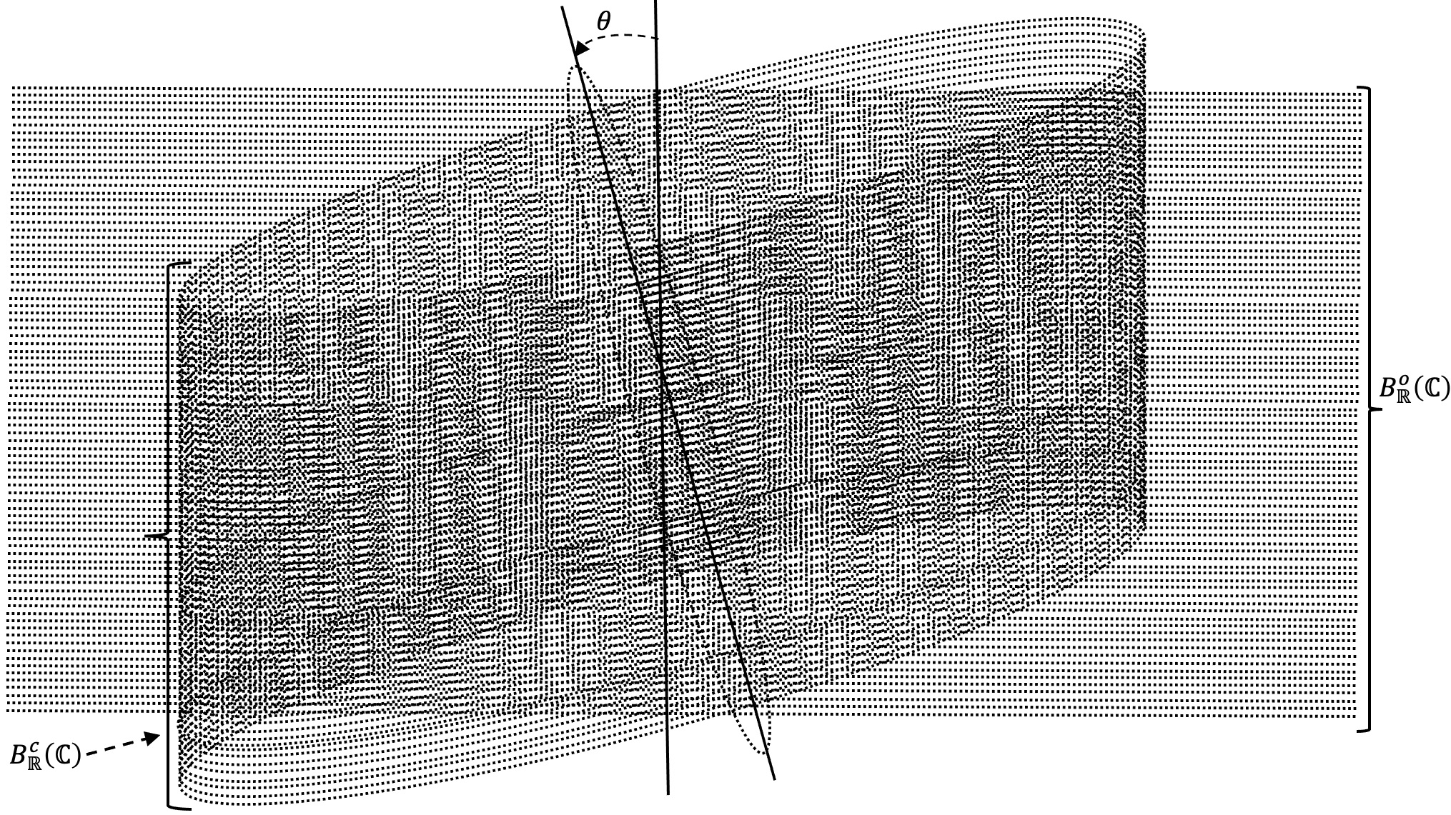
Figure 2.5. Angle between two bundles $B_{\mathbb{R}}^{o}(\mathbb{C})$ and $B_{\mathbb{R}}^{c}(\mathbb{C})$ and rotation of the bundle $B_{\mathbb{R}}^{c}(\mathbb{C})$ over $y-$axis.

Statement (2.33) is true for every $\theta>0$ and every $B_{\mathbb{R}}^{c}(\mathbb{C},\theta).$ Since $\theta$ is arbitrary, the statement (2.33) is true for each $\theta\in(0,360].$ Hence, the space created by $B_{\mathbb{R}}^{c}(\mathbb{C},\theta)$ for all $\theta$ values for $\theta\in(0,360^{0}]$ is the same as the space of the bundle $B_{\mathbb{R}}(\mathbb{C}).$ ∎

Remark 6.

The $n-$dimensional complex plane $\mathbb{C}^{n}$ is also subset of the space created by the rotation in the Theorem 5.

3. Multilevel Contours in a Random Environment

Let us consider the bundle $B_{\mathbb{R}}(\mathbb{C})$ combined with the $\mathbb{C}_{0}$ intersecting with the bundle as in Section 2. Let the intersection of $\mathbb{C}_{0}$ on the bundle be arbitrary. Choose a plane $\mathbb{C}_{l}$ for $\mathbb{C}_{l}\in B_{\mathbb{R}}(\mathbb{C}).$ Let $X\left(\gamma_{l},\mathbb{C}_{l}\right)$ be a random variable describing the position of the complex number on a contour $\gamma_{l}$ at time $t$ in the plane $\mathbb{C}_{l}$. Here $\gamma_{l}$ is described by $z_{l}(t)$ $(t_{0}\leq t\leq b_{0})$ for $t_{0},b_{0}\in\mathbb{R}$ and $z_{l}(t_{0})=$ $z_{l_{0}}$, say. Let $X\left(z_{l_{0}},\mathbb{C}_{l}\right)$ be the position of the random variable at $t_{0}$ in $\mathbb{C}_{l}$. Here $X\left(\gamma_{l},\mathbb{C}_{l}\right)$ can be treated like a standard measurable function. Suppose $X\left(z_{l_{0}},\mathbb{C}_{l}\right)$ picked arbitrarily in the plane $\mathbb{C}_{l}$. Here $X\left(z_{l}(t),\mathbb{C}_{l}\right)$ for $t\in[t_{0},\infty)$ and $z_{l}(t)\in\mathbb{C}_{l}$ is a stochastic process on the complex plane $\mathbb{C}_{l}$. Once $X\left(z_{l_{0}},\mathbb{C}_{l}\right)$ is chosen, the location of $X\left(z_{l_{1}},\mathbb{C}_{l}\right)$ for $t_{1}>t_{0}$ could be anywhere within an open disc $D\left(z_{l_{0}}.r_{0}\right)$, where $X\left(z_{l_{1}},\mathbb{C}_{l}\right)$ is the complex number picked by $X\left(z_{l}(t),\mathbb{C}_{l}\right)$ at $t_{1}$ and

$$D\left(z_{l_{0}}.r_{0}\right)=\left\{z:\left|z-z_{l_{0}}\right|<r_{0}\text{ for $r_{0}>0$ and }z\in\mathbb{C}_{l}\right\}.$$

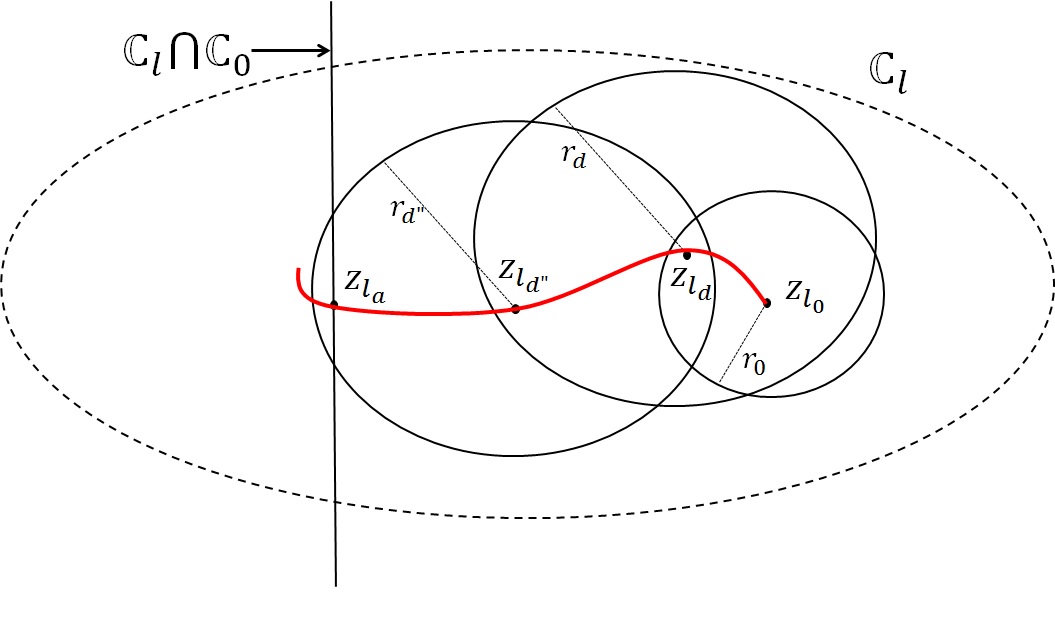
Figure 3.1. Formation of contours through two-step randomness.

Suppose $X\left(z_{l_{0}},\mathbb{C}_{l}\right)=z_{l_{1}}$. The selection of radius is done randomly at each step of selecting a complex number. Once $X\left(z_{l},\mathbb{C}_{l}\right)$ chooses a number at $t_{0}$ then during $[t_{0},t_{1}]$ a value for $r_{0}$ for $r_{0}>0$ is chosen randomly to build $D\left(z_{l_{0}}.r_{0}\right).$ Once the set of points of $D\left(z_{l_{0}}.r_{0}\right)$ are available then $X\left(z_{l_{0}},\mathbb{C}_{l}\right)$ will choose the second number during $[t_{0},t_{1}].$ See Figure 3.1. This procedure of two-step randomness continues forever in the intervals

$$\left\{[t_{0},t_{a}],(t_{a},t_{a^{\prime}}],(t_{a^{\prime}},t_{b}],(t_{b},t_{b^{\prime}],...}\right\}$$

where $a,a^{\prime},b,b^{\prime},...\in\mathbb{R}$ and $t_{0}<t_{a}<t_{a^{\prime}}<t_{b}<t_{b^{\prime}<...}.$ We can draw a contour from $z_{l_{0}}$to $z_{l_{1}}$ using the set of points generated by $z_{l}(t)$ within the time interval $[t_{0},t_{1})$. The set of all possible values the set $\left\{X\left(z_{l},\mathbb{C}_{l}\right)\right\}$ can take over the interval $t_{0},\infty)$ is called the state-space of $X\left(z_{l}(t),\mathbb{C}_{l}\right).$ This continuous-time stochastic process does not stop once the initial value on the plane $\mathbb{C}_{l}$ is chosen and its state-space is $\mathbb{C}_{l}$. The described process is a continuous time and continuous space stochastic process. Let $p\left(z_{l}(t_{1}),\mathbb{C}_{l}\right)$ be the probability function that is associated with $X\left(z_{l}(t_{1}),\mathbb{C}_{l}\right)$ such that $p\left(z_{l}(t_{1}),\mathbb{C}_{l}\right)$ describes the probability that $X\left(z_{l}(t_{1}),\mathbb{C}_{l}\right)$ picks $z_{l_{1}}$for $z_{l_{1}}=z_{l}(t_{1})$ $(t_{1}>t_{0}).$ The probability function defined as

(3.1) $$p\left(z_{l}(t_{1}),t_{1}\right)=\text{Prob}\left[X\left(z_{l}(t_{1}),\mathbb{C}_{l}\right)=z_{l_{1}}\right]\text{ for }t_{1}>t_{0}.$$

Once $X\left(z_{l}(t_{1}),\mathbb{C}_{l}\right)$ is generated, then one can draw contour from $z_{l_{0}}$to $z_{l_{1}}$and compute $L(z_{l_{0}},z_{l_{1}})$ the length from $z_{l_{0}}$to $z_{l_{1}}$. The contour $\gamma_{l}$ is described by

$$\gamma_{l}=z_{l}(t)\text{ for }t\in[t_{0},\infty)$$

and

$$t=v_{l}(\tau)\text{ }\left(a_{0}^{l_{0}}\leq t<a_{0}^{l_{1}}\right)$$

is the parametric representation for $\gamma_{l}$ with a real valued function $v_{l}$ mapping $[a_{0}^{l_{0}},a_{0}^{l_{1}})$ onto the interval $[t_{0},t_{1}).$ This gives us,

(3.2) $$L(z_{l_{0}},z_{l_{1}})=\int_{a_{0}^{l_{0}}}^{a_{0}^{l_{1}}}\left|z\left[v_{l}(\tau)\right]\right|v^{\prime}_{l}(\tau)d\tau.$$

Our main focus here in this article is on multilevel contours. So initially we assume that once the variable $X\left(z_{l}(t_{1}),\mathbb{C}_{l}\right)$ is picked a value at $t_{0}$, it can not reach the same value for $t>t_{0},$ i.e.,

(3.3) $$X\left(z_{l}(t_{0}),\mathbb{C}_{l}\right)\neq X\left(z_{l}(t),\mathbb{C}_{l}\right)\text{ for }t>t_{0}.$$

For simplicity in understanding, we might denote (at certain specific places in the article) a complex number generated at each iteration with an integer index. However, in reality the numbers chosen by $X\left(z_{l}(t),\mathbb{C}_{l}\right)$ are uncountably infinite.

Definition 7.

Distinct complex numbers by $X\left(z_{l}(t),\mathbb{C}_{l}\right)$: Suppose $X\left(z_{l}(t_{0}),\mathbb{C}_{l}\right)=z_{l_{0}}$ for $z_{l_{0}}\in\mathbb{C}_{l}.$ Suppose $X\left(z_{l}(t),\mathbb{C}_{l}\right)=z_{l_{\alpha}}$ for $t\in[t_{0},t_{\alpha}]$ and $X\left(z_{l}(t),\mathbb{C}_{l}\right)=z_{l_{\beta}}$ for $t\in(t_{\alpha},t_{\beta}]$ for all $t_{0}<t_{\alpha}<t_{\beta}$, and $\alpha,\beta,$$t_{0},t_{\alpha},t_{\beta}\in\mathbb{R}$ then $z_{l_{0}}\neq z_{l_{\alpha}}\neq z_{l_{\beta}}.$ This property assures that $X\left(z_{l}(t),\mathbb{C}_{l}\right)$ cannot choose the same number that it already chose in any of the previous time intervals after the initial number is chosen (including the initial number).

When a random variable $X\left(z_{l}(t),\mathbb{C}_{l}\right)$ chooses a number within the disc created and that value (number) has been chosen already and was part of the contour, then, $X\left(z_{l}(t),\mathbb{C}_{l}\right)$ will choose another number in the disc. This procedure continues until a distinct number is chosen by $X\left(z_{l}(t),\mathbb{C}_{l}\right)$. Such an assumption in (7) or in (3.3) will allow quicker formation of multilevel contour. We will later see the consequences of relaxing the assumption in (7). We have

(3.4) $$z_{l_{1}}\in D\left(z_{l_{0}}.r_{0}\right)\text{ and }z_{l_{0}}\neq z_{l_{1}}.$$

Let $z_{l}(t_{2})$ be the value of $X\left(z_{l}(t_{1}),\mathbb{C}_{l}\right)$ at $t_{2}$ for $t_{2}>t_{1}$ and $z_{l}(t_{2})\in D\left(z_{l_{1}}.r_{1}\right)$ for $r_{1}>0$ such that

$$p\left(z_{l}(t_{2}),t_{2}\right)=\text{Prob}\left[X\left(z_{l}(t_{1}),\mathbb{C}_{l}\right)=z_{l_{2}}\right]\text{ for }t_{2}>t_{1}.$$

The contour $\gamma_{l}$ with a new parametric representation

$$t=v_{l}(\tau)\text{ }\left(a_{0}^{l_{1}}\leq t<a_{0}^{l_{2}}\right)$$

with a real valued function $v_{l}$ mapping $[a_{0}^{l_{1}},a_{0}^{l_{2}})$ onto the interval $[t_{1},t_{2})$ helps us to compute the length $L(z_{l_{1}},z_{l_{2}})$ from $z_{l_{1}}$to $z_{l_{2}}=z_{l}(t_{2})$ from $z_{l_{1}}$ for $t_{2}>t_{1}.$ That is,

$$p\left(z_{l}(t_{2}),t_{2}\right)= \text{Prob}\left[X\left(z_{l}(t_{2}),\mathbb{C}_{l}\right)=z_{l}(t_{2})/X\left(z_{l}(t_{0}),\mathbb{C}_{l}\right)=z_{l_{0}},\right.$$

$$\left.X\left(z_{l}(t_{1}),\mathbb{C}_{l}\right)=z_{l}(t_{1})\right]$$

(3.5) $$L(z_{l_{1}},z_{l_{2}})=\int_{a_{0}^{l_{1}}}^{a_{0}^{l_{2}}}\left|z\left[v_{l}(\tau)\right]\right|v^{\prime}_{l}(\tau)d\tau.$$

Note that, we are not drawing contours from $z_{l_{0}}$to $z_{l_{2}}$ because $X\left(z_{l}(t_{1}),\mathbb{C}_{l}\right)$ will change to $z_{l_{2}}$for $t_{2}>t_{1}.$ In fact, under the construction explained, the contour will start $z_{l_{0}}$and reach $z_{l_{2}}$only through the point $z_{l_{1}}.$ As these are new ideas, we have explained above the probabilities of picking various values by $X\left(z_{l}(t_{1}),\mathbb{C}_{l}\right)$. We will slightly re-define below the probabilities and their transitions to accommodate an easier understanding of these concepts.

There are infinitely many options around $z_{l_{0}}$ that $X\left(z_{l}(t_{1}),\mathbb{C}_{l}\right)$ can pick during $[t_{0},t_{1}]$ each with a probability $p\left(z_{l}(t),t\right)$ for $t\in[t_{0},t_{1}].$ Let $p\left(z_{l_{0}},z_{l}(t),t\right)$ for $t\in[t_{0},t_{1}]$ that $X\left(z_{l}(t),\mathbb{C}_{l}\right)$ =$z_{l_{0}}$at $t_{0}$ has transitioned to $X\left(z_{l}(t),\mathbb{C}_{l}\right)$ =$z_{l_{1}}$at during $[t_{0},t_{1}].$ For all such probabilities of transitions during $[t_{0},t_{1}]$, we will have

(3.6) $$\int_{t_{0}}^{t_{1}}p\left(z_{l_{0}},z_{l}(t),t\right)dt=1,$$

where $p\left(z_{l_{0}},z_{l}(t),t\right)$ can be expressed as

$$p\left(z_{l_{0}},z_{l}(t),t\right)=\text{Prob}\left[X\left(z_{l}(t),\mathbb{C}_{l}\right)=z_{l_{1}}\left/X\left(z_{l}(t_{0}),\mathbb{C}_{l}\right)=z_{l_{0}}\right.\right].$$

Let $p\left(z_{l_{0}},z_{l}(t),t\right)$ for $t\in(t_{1},t_{2}]$ be the probability that $X\left(z_{l}(t),\mathbb{C}_{l}\right)$ during $(t_{1},t_{2}]$ will pick a number within $D(z_{l_{1}},r_{1})$$\in\mathbb{C}_{l}$ among infinitely many options. The transition probability from $z_{l_{1}}$ to $z_{l_{2}}$during $(t_{1},t_{2}]$ is

$$p\left(z_{l_{1}},z_{l}(t),t\right)\text{ }\left(t\in(t_{1},t_{2}]\right)=\text{Prob}[X\left(z_{l}(t),\mathbb{C}_{l}\right)=z_{l_{2}}\left/X\left(z_{l}(t_{1}),\mathbb{C}_{l}\right)=z_{l_{1}}\right.]$$

such that

$$\int_{t_{1}}^{t_{2}}p\left(z_{l_{1}},z_{l}(t),t\right)dt=1.$$

Note that,

$$p\left(z_{l_{0}},z_{l}(t),t\right)\text{ }\left(t\in[t_{0},t_{2}]\right) =$$

$$p\left(z_{l_{0}},z_{l}(t),t\right)\text{ }\left(t\in[t_{0},t_{1}]\right)\times$$

(3.7) $$p\left(z_{l_{1}},z_{l}(t),t\right)\text{ }\left(t\in(t_{0},t_{2}]\right).$$

A direct transition from the complex number $z_{l_{0}}$ to another complex number $z_{l_{2}}$is not possible during $[t_{0},t_{2}]$ under the above framework. A direct transition we mean here a one-step transition. As $X\left(z_{l}(t),\mathbb{C}_{l}\right)$ has reached $z_{l_{1}}$during $[t_{0},t_{1}]$ and then $X\left(z_{l}(t),\mathbb{C}_{l}\right)$ starting at $z_{l_{1}}$it has taken the value $z_{l_{2}}$ during $(t_{1},t_{2}].$ This implies, $p\left(z_{l_{0}},z_{l}(t),t\right)\text{ }\left(t\in[t_{0},t_{2}]\right)$ is not possible without having a hopping over the value $X\left(z_{l}(t),\mathbb{C}_{l}\right)=z_{l_{1}}$ during $[t_{0},t_{1}].$ If $z_{l_{2}}$is not picked by $X\left(z_{l}(t),\mathbb{C}_{l}\right)$ during $(t_{1},t_{2}]$ then it can be picked at some future time by $X\left(z_{l}(t),\mathbb{C}_{l}\right)$ for $t>t_{2}.$ So,

$$p\left(z_{l_{0}},z_{l}(t),t\right)\text{ }\left(t\in[t_{0},t_{2}]\right)=\begin{cases}\begin{array}[]{cc}0&\text{(one-step transition)}\\ >0&\text{(two or more-steps transitions)}\end{array}\end{cases}$$

Theorem 8.

A contour formed by the set of points generated by $X\left(z_{l}(t),\mathbb{C}_{l}\right)$ on $\mathbb{C}_{l}$ for $\mathbb{C}_{l}$ in the bundle $B_{\mathbb{R}}(\mathbb{C})$ combined with the $\mathbb{C}_{0}$ intersecting with the bundle and satisfying (7) will obey continuous time Markov property.

Proof.

Let $\gamma_{l}$ be the contour generated by $X\left(z_{l}(t),\mathbb{C}_{l}\right)$ over the time interval $[t_{0},\infty).$ Suppose $X\left(z_{l}(t_{0}),\mathbb{C}_{l}\right)=z_{l_{0}}.$ Suppose $X\left(z_{l}(t),\mathbb{C}_{l}\right)$ has taken the value $z_{l_{1}}$during $t\in[t_{0},t_{1}],$ and $X\left(z_{l}(t),\mathbb{C}_{l}\right)$ has taken the value $z_{l_{2}}$during $t\in(t_{1},t_{2}].$ Here $z_{l_{1}}\in D\left(z_{l_{0}}.r_{0}\right)\subset\mathbb{C}_{l}$ for $r_{0}>0,$ and $z_{l_{2}}\in D\left(z_{l_{1}}.r_{1}\right)\subset\mathbb{C}_{l}$ for $r_{1}>0.$ By this construction, we have

$$D\left(z_{l_{0}}.r_{0}\right)\cap D\left(z_{l_{1}}.r_{1}\right)\neq\phi\text{ (empty set)}$$

Since (7) holds, we have $z_{l_{1}}\neq z_{l_{0}}.$ The transition probability for $X\left(z_{l}(t),\mathbb{C}_{l}\right)$ from $z_{l_{0}}$to $z_{l_{2}}$is

$$p(z_{l_{0}},z_{l_{2}},t)\text{}\left(t\in[t_{0},t_{2}]\right)=p(z_{l_{0}},z_{l_{1}},t)\text{}\left(t\in[t_{0},t_{1}]\right)\text{ and }p(z_{l_{1}},z_{l_{2}},t)\text{}\left(t\in(t_{1},t_{2}]\right)$$

$$=\text{Prob}[X\left(z_{l}(t),\mathbb{C}_{l}\right)=z_{l_{1}}\text{}\left(t\in[t_{0},t_{1}]\right)\left/X\left(z_{l}(t_{0}),\mathbb{C}_{l}\right)=z_{l_{0}}]\times\right.$$

$$\text{ }\text{Prob}[X\left(z_{l}(t),\mathbb{C}_{l}\right)=z_{l_{2}}\text{}\left(t\in(t_{1},t_{2}]\right)\left/X\left(z_{l}(t),\mathbb{C}_{l}\right)=z_{l_{1}}\text{}\left(t\in[t_{0},t_{1}]\right)]\right.$$

Through (LABEL:eq:MCin=00005Bt0,t2=00005D), we can conclude that the random variable $X\left(z_{l}(t),\mathbb{C}_{l}\right)$ $\text{}\left(t\in[t_{0},t_{2}]\right)$ obeys Markov property during the interval $[t_{0},t_{2}].$ In (LABEL:eq:MCin=00005Bt0,t2=00005D), the number $z_{l_{2}}$is generated within a disc around the number $z_{l_{1}}$but not around the disc with center $z_{l_{0}}.$ A contour is drawn from $z_{l_{0}}$ to $z_{l_{2}}$only through $z_{l_{1}}.$ In a similar way, the value of $X\left(z_{l}(t),\mathbb{C}_{l}\right)\text{}\left(t\in(t_{n-1},t_{n}]\right)$ is located in the disc $D\left(z_{l_{n-1}}.r_{n-1}\right)$ for $r_{n-1}>0$ and not on the discs $D\left(z_{l_{k}}.r_{k}\right)$ for $r_{k}>0$ and $k=0,1,...,n-2.$ That is,

$$\text{Prob}[X\left(z_{l}(t),\mathbb{C}_{l}\right)=z_{l_{n}}\text{}\left(t\in(t_{n-1},t_{n}]\right)\left/X\left(z_{l}(t_{0}),\mathbb{C}_{l}\right)=z_{l_{0}},X\left(z_{l}(t),\mathbb{C}_{l}\right)=z_{l_{1}}\right.$$

$$X\left(z_{l}(t),\mathbb{C}_{l}\right) =z_{l_{1}}\text{}\left(t\in(t_{0},t_{1}]\right),...,...,X\left(z_{l}(t),\mathbb{C}_{l}\right)=z_{l_{n-1}}\text{}\left(t\in(t_{n-2},t_{n-1}]\right)]$$

$$=\text{Prob}[X\left(z_{l}(t),\mathbb{C}_{l}\right)=z_{l_{n}}\text{}\left(t\in(t_{n-1},t_{n}]\right)\left/\right.$$

(3.9) $$X\left(z_{l}(t),\mathbb{C}_{l}\right)=z_{l_{n-1}}\text{}\left(t\in(t_{n-2},t_{n-1}]\right)]$$

A contour is drawn from $z_{l_{0}}$ to $z_{l_{n}}$only connecting the numbers (points) through $z_{l_{1}},z_{l_{2}},...,$ $z_{l_{n-1}}.$ The result in (3.9) is also true when $t_{n}\rightarrow\infty.$ Hence the contour $\gamma_{l}$ is formed using the numbers generated by $X\left(z_{l}(t),\mathbb{C}_{l}\right)$ $\text{}\left(t\in[t_{0},\infty]\right)$ obeys properties of continuous time Markov property or obeys continuous time Markov chain. ∎

3.1. Behavior of $X\left(z_{l}(t),\mathbb{C}_{l}\right)$ at $\left(\mathbb{C}_{l}\cap\mathbb{C}_{0}\right).$

Let us understand the behavior of $X\left(z_{l}(t),\mathbb{C}_{l}\right)$ at the intersection of $\mathbb{C}_{l}\cap\mathbb{C}_{0}.$ Set $\mathbb{C}_{l}\cap\mathbb{C}_{0}$ consists of elements $\mathbb{C}_{l}\cap\mathbb{C}_{0}=\left\{z:z\in\mathbb{C}_{l}\text{ and }z\in\mathbb{C}_{0}\right\}.$ Here $\mathbb{C}_{l}\cap\mathbb{C}_{0}\neq\phi\text{ (empty).}$ The numbers on $\mathbb{C}_{l}\cap\mathbb{C}_{0}$ form a dense set of numbers and they form a line. Whenever $X\left(z_{l}(t),\mathbb{C}_{l}\right)$ reaches a number, say, $z_{l_{a}}$ in the set $\mathbb{C}_{l}\cap\mathbb{C}_{0}$, then $X\left(z_{l}(t),\mathbb{C}_{l}\right)$ can choose the next number within the set $\mathbb{C}_{l}\cap\mathbb{C}_{0}$ or within the plane $\mathbb{C}_{l}$ or within the plane $\mathbb{C}_{0}.$ That is, as soon as $X\left(z_{l}(t),\mathbb{C}_{l}\right)$ chooses a number $z_{l_{a}}$after a countable number of transitions from $z_{l_{0}},$ then the two-step randomness will help to form two discs, namely, $D\left(z_{l_{a}},r_{a},\mathbb{C}_{l}\right)$ and $D\left(z_{l_{a}},r_{a},\mathbb{C}_{0}\right).$ Here

(3.10) $$D\left(z_{l_{a}},r_{a},\mathbb{C}_{l}\right)\subset\mathbb{C}_{l}\text{ and }D\left(z_{l_{a}},r_{a},\mathbb{C}_{0}\right)\subset\mathbb{C}_{0}.$$

One can have different radii for two discs. For both the discs we leave the the symbol $z_{l_{a}}$ in both the discs to indicate that the associated random variable has origins in $\mathbb{C}_{l}.$ The next number of $X\left(z_{l}(t),\mathbb{C}_{l}\right)$, say, $z_{l_{b}}$ could fall within $D\left(z_{l_{a}},r_{a},\mathbb{C}_{l}\right)$ such that it is on line $\mathbb{C}_{l}\cap\mathbb{C}_{0}$ or it is in the set $\mathbb{C}_{l}\cap\left(\mathbb{C}_{l}\cap\mathbb{C}_{0}\right)^{\prime}$. Alternatively, $z_{l_{b}}$ could fall within $D\left(z_{l_{a}},r_{a},\mathbb{C}_{0}\right)$ such that it is on line $\mathbb{C}_{l}\cap\mathbb{C}_{0}$ or it is in the set $\mathbb{C}_{0}\cap\left(\mathbb{C}_{l}\cap\mathbb{C}_{0}\right)^{\prime}$where

$$\mathbb{C}_{l}\cap\left(\mathbb{C}_{l}\cap\mathbb{C}_{0}\right)^{\prime} =\left\{z:z\in\mathbb{C}_{l}\text{ and }z\notin\left(\mathbb{C}_{l}\cap\mathbb{C}_{0}\right)\right\}$$

(3.11) $$\mathbb{C}_{0}\cap\left(\mathbb{C}_{l}\cap\mathbb{C}_{0}\right)^{\prime} =\left\{z:z\in\mathbb{C}_{0}\text{ and }z\notin\left(\mathbb{C}_{l}\cap\mathbb{C}_{0}\right)\right\}.$$

If $z_{l_{b}}\in\mathbb{C}_{0}\cap\left(\mathbb{C}_{l}\cap\mathbb{C}_{0}\right)^{\prime}$, then by joining all the numbers generated by $X\left(z_{l}(t),\mathbb{C}_{l}\right)$ from$z_{l_{0}}$ through $z_{l_{b}},$ we form a multilevel contour. If $z_{l_{b}}\in\mathbb{C}_{l}\cap\left(\mathbb{C}_{l}\cap\mathbb{C}_{0}\right)^{\prime}$, then by joining all the numbers generated by $X\left(z_{l}(t),\mathbb{C}_{l}\right)$ from$z_{l_{0}}$ through $z_{l_{b}},$ we form a contour on $\mathbb{C}_{l}$. Even if $z_{l_{b}}\in\mathbb{C}_{l}\cap\left(\mathbb{C}_{l}\cap\mathbb{C}_{0}\right)^{\prime}$, still $X\left(z_{l}(t),\mathbb{C}_{l}\right)$ can choose at a future iteration a value (number) in the set $\left(\mathbb{C}_{l}\cap\mathbb{C}_{0}\right)$ and escape the plane through $\mathbb{C}_{0}.$ Again at a future iteration the value of $X\left(z_{l}(t),\mathbb{C}_{l}\right)$ could fall within $\mathbb{C}_{l}.$ As soon as $X\left(z_{l}(t),\mathbb{C}_{l}\right)$ leaves $\mathbb{C}_{l}$ (if in case) it reaches another plane, say, $\mathbb{C}_{p},$ because $\left(\mathbb{C}_{p}\cap\mathbb{C}_{0}\right)\neq\phi$ and $\left(\mathbb{C}_{p}\cap\mathbb{C}_{0}\right)\subset\mathbb{C}_{p}$ for some elements of $\mathbb{C}_{0}.$ Anytime $X\left(z_{l}(t),\mathbb{C}_{l}\right)$ reaches a set of intersecting planes $\left(\mathbb{C}_{l}\cap\mathbb{C}_{0}\right)$ or $\left(\mathbb{C}_{p}\cap\mathbb{C}_{0}\right)$ or some other similar intersecting planes, it will have the power to generate next number in two distinct discs as described above in (). This feature of $X\left(z_{l}(t),\mathbb{C}_{l}\right)$ helps to form multilevel contours. This feature is summarized below:

$$X\left(z_{l}(t),\mathbb{C}_{l}\right)=z_{l_{b}}\text{ and }z_{l_{b}}\in D\left(z_{l_{a}},r_{a},\mathbb{C}_{0}\right) \implies\gamma_{l}\text{ is a multilevel contour}$$

$$X\left(z_{l}(t),\mathbb{C}_{l}\right)=z_{l_{b}}\text{ and }z_{l_{b}}\in D\left(z_{l_{a}},r_{a},\mathbb{C}_{l}\right) \implies\gamma_{l}\text{ is a contour on }\mathbb{C}_{l}$$

This rule (LABEL:eq:intersectionRULES) is applicable to the each time the value of $X\left(z_{l}(t),\mathbb{C}_{l}\right)$ falls in an intersection of planes. Once a contour attains the multilevel contour property it will remain as a multilevel contour of that particular $X\left(z_{l}(t),\mathbb{C}_{l}\right)$ even if the value of $X\left(z_{l}(t),\mathbb{C}_{l}\right)$ reruns and remains in $\mathbb{C}_{l}$ forever. The value of the radius at each two-step randomness and the location of the next number to be picked by $X\left(z_{l}(t),\mathbb{C}_{l}\right)$ decides the time taken for a contour to become a multilevel contour (if there is a possibility to become). See Figure 3.2.The time interval to reach $z_{l_{a}}$ from $z_{l_{0}}$ could be at least one, and it requires at least two time interval to reach $z_{l_{b}}$ from $z_{l_{0}}$ under the framework described above.

Suppose $z_{l_{b}}\in D\left(z_{l_{a}},r_{a},\mathbb{C}_{0}\right)^{\prime}$. If $z_{l_{0}}$ to $z_{l_{a}}$ reaches in one time interval and $z_{l_{a}}$ to $z_{l_{b}}$ reaches in one time interval then

$$\left\|z_{l_{b}}-z_{l_{0}}\right\|>\left\|z_{l_{a}}-z_{l_{0}}\right\|$$

because

$$\left\|z_{l_{a}}-z_{l_{0}}\right\|+\left\|z_{l_{a}}-z_{l_{b}}\right\|=\left\|z_{l_{b}}-z_{l_{0}}\right\|$$

If $z_{l_{0}}$ to $z_{l_{a}}$ reaches in more than one time interval, then the length of the contour, $L(z_{l_{o}},z_{l_{a}})$ from $z_{l_{0}}$to $z_{l_{a}}$ is still less than $L(z_{l_{o}},z_{l_{b}})$ from $z_{l_{0}}$to $z_{l_{b}}$ because $z_{l_{b}}$ lies in the disc $D\left(z_{l_{a}},r_{a},\mathbb{C}_{0}\right)^{\prime}.$ Suppose $X\left(z_{l}(t_{0}),\mathbb{C}_{l}\right)=z_{l_{0}}$ and $X\left(z_{l}(t),\mathbb{C}_{l}\right)$ reaches at $z_{l_{a}}$during the $n^{th}$ time interval. Let $X\left(z_{l}(t),\mathbb{C}_{l}\right)=z_{l_{1}}$ for $z_{l_{1}}\in D\left(z_{l_{0}}.r_{0}\right)$ during the first time interval $[t_{0},t_{1}]$ and $X\left(z_{l}(t),\mathbb{C}_{l}\right)=z_{l_{2}}$ for $z_{l_{2}}\in D\left(z_{l_{1}}.r_{1}\right)$ during the second time interval and so on $X\left(z_{l}(t),\mathbb{C}_{l}\right)=z_{l_{a}}$ for $z_{l_{a}}\in D\left(z_{l_{n-1}}.r_{n-1}\right)$ during $n^{th}$ time interval. Suppose $X\left(z_{l}(t),\mathbb{C}_{l}\right)=z_{l_{b}}$ for $z_{l_{b}}\in D\left(z_{l_{a}}.r_{a}\right).$ Suppose $\gamma_{l}$ is described by

$$\gamma_{l}=z_{l}(t)\text{ for }t\in[t_{0},\infty)$$

and the parametric representations are given by

$$\begin{array}[]{cc}t=&\left\{\begin{array}[]{c}v_{l_{1}}(\tau)\text{ }\left(a_{0}^{l_{0}}\leq t\leq a_{0}^{l_{1}}\right)\\ v_{l_{2}}(\tau)\text{ }\left(a_{0}^{l_{1}}<t\leq a_{0}^{l_{2}}\right)\\ \vdots\\ v_{l_{n-1}}(\tau)\text{ }\left(a_{0}^{l_{n-2}}<t\leq a_{0}^{l_{n-1}}\right)\\ v_{l_{a}}(\tau)\text{ }\left(a_{0}^{l_{n-1}}<t\leq a_{0}^{l_{a}}\right)\\ v_{l_{b}}(\tau)\text{ }\left(a_{0}^{l_{a}}<t\leq a_{0}^{l_{b}}\right)\\ \\ \end{array}\right.\end{array},$$

and the real valued functions $v_{l_{i+1}}$ mapping $(a_{0}^{l_{i}},a_{0}^{l_{i+1}}]$ for $i=1,...,n-2$ onto the intervals $[t_{0},t_{1}],$ $(t_{1},t_{2}],$ $(t_{n-2},t_{n-1}].$ The real valued function $v_{l_{0}}$ maps $[a_{0}^{l_{0}},a_{0}^{l_{1}}]$ onto the interval $([t_{0},t_{1}]$, $v_{l_{a}}$ maps $(a_{0}^{l_{n-1}},a_{0}^{l_{a}}]$ onto the interval $(t_{n-1},t_{a}]$ and the real valued function $v_{l_{b}}$ maps $(a_{0}^{l_{a}},a_{0}^{l_{b}}]$ onto the interval $(t_{a},t_{b}].$ Then

$$L(z_{l_{o}},z_{l_{b}}) =\sum_{i=1}^{n-1}\int_{a_{0}^{l_{i}}}^{a_{0}^{l_{i+1}}}\left|z\left[v_{l_{i}}(\tau)\right]\right|v^{\prime}_{l_{i}}(\tau)d\tau+\int_{a_{0}^{l_{n-1}}}^{a_{0}^{l_{a}}}\left|z\left[v_{l_{a}}(\tau)\right]\right|v^{\prime}_{l_{a}}(\tau)d\tau$$

(3.13) $$+\int_{a_{0}^{l_{a}}}^{a_{0}^{l_{b}}}\left|z\left[v_{l_{b}}(\tau)\right]\right|v^{\prime}_{l_{b}}(\tau)d\tau$$

$$>L(z_{l_{o}},z_{l_{a}})$$

because the first two terms of the R.H.S. of (3.13) is $L(z_{l_{o}},z_{l_{a}}).$ Here

$$\int_{a_{0}^{l_{i}}}^{a_{0}^{l_{i+1}}}\left|z\left[v_{l_{i}}(\tau)\right]\right|v^{\prime}_{l_{i}}(\tau)d\tau \subset D\left(z_{l_{i}},r_{i}\right)\text{ for }i=1,2,...,n-1$$

$$\int_{a_{0}^{l_{n-1}}}^{a_{0}^{l_{a}}}\left|z\left[v_{l_{a}}(\tau)\right]\right|v^{\prime}_{l_{a}}(\tau)d\tau \subset D\left(z_{l_{n-1}},r_{a},\mathbb{C}_{l}\right)$$

$$\int_{a_{0}^{l_{a}}}^{a_{0}^{l_{b}}}\left|z\left[v_{l_{b}}(\tau)\right]\right|v^{\prime}_{l_{b}}(\tau)d\tau \subset D\left(z_{l_{a}},r_{a},\mathbb{C}_{0}\right)$$

and

$$D\left(z_{l_{0}},r_{0}\right)\cap D\left(z_{l_{1}},r_{1}\right)\cap...\cap D\left(z_{l_{n-2}},r_{n-2}\right)\neq\phi\text{ (empty)}$$

each of these discs are non-empty and they have distinct set of numbers on $\mathbb{C}_{l}.$ The disc $D\left(z_{l_{a}},r_{a},\mathbb{C}_{0}\right)$ has some elements outside the plane $\mathbb{C}_{l}$, and

$$D\left(z_{l_{n-1}},r_{n-1},\mathbb{C}_{l}\right)\cap D\left(z_{l_{a}},r_{a},\mathbb{C}_{0}\right)\neq\phi\text{ (empty)}.$$

Suppose it takes infinitely many time intervals to reach $z_{l_{a}}$ from $z_{l_{0}}$ (due to the random environment created).

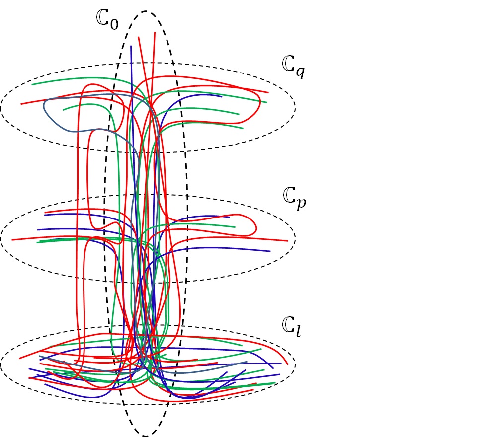
Figure 3.2. Contours spreading across one or more planes from $\mathbb{C}_{l}$ due to random environment.

Extending the parametric representation described above, the length of the contour from $z_{l_{0}}$ to $z_{l_{a}}$is

$$L(z_{l_{o}},z_{l_{a}})=\sum_{i=1}^{\infty}\int_{a_{0}^{l_{i}}}^{a_{0}^{l_{\infty}}}\left|z\left[v_{l_{i}}(\tau)\right]\right|v^{\prime}_{l_{i}}(\tau)d\tau<L(z_{l_{o}},z_{l_{b}})$$

because

$$L(z_{l_{o}},z_{l_{b}})=\sum_{i=1}^{\infty}\int_{a_{0}^{l_{i}}}^{a_{0}^{l_{\infty}}}\left|z\left[v_{l_{i}}(\tau)\right]\right|v^{\prime}_{l_{i}}(\tau)d\tau+\int_{a_{0}^{l_{\infty}}}^{a_{0}^{l_{b}}}\left|z\left[v_{l_{b}}(\tau)\right]\right|v^{\prime}_{l_{b}}(\tau)d\tau$$

and

$$\int_{a_{0}^{l_{\infty}}}^{a_{0}^{l_{b}}}\left|z\left[v_{l_{b}}(\tau)\right]\right|v^{\prime}_{l_{b}}(\tau)d\tau\subset D\left(z_{l_{\infty}},r_{\infty},\mathbb{C}_{0}\right)$$

(3.14) $$\bigcap_{i=0}^{\infty}D\left(z_{l_{i}},r_{i}\right)\neq\phi\text{ (empty)}.$$

Theorem 9.

Suppose it takes infinitely many time intervals for $X\left(z_{l}(t),\mathbb{C}_{l}\right)$ to reach $z_{l_{a}}$ from $z_{l_{0}}$ The infinitely many discs (uncountable) created while reaching $z_{l_{a}}$from $z_{l_{0}}$ could be nested under the two-step random environment created by $X\left(z_{l}(t),\mathbb{C}_{l}\right)$ and $\bigcap_{i=0}^{\infty}D\left(z_{l_{i}},r_{i}\right)\neq\phi.$

Proof.

Suppose $X\left(z_{l}(t_{0}),\mathbb{C}_{l}\right)=z_{l_{0}}.$ Let $D\left(z_{l_{0}},r_{0}\right)$ formed out of two-step randomness and $z_{l_{1}}\in D\left(z_{l_{0}},r_{0}\right).$ Suppose $r_{1}$ is generated randomly such that $D\left(z_{l_{1}},r_{1}\right)$$\subset D\left(z_{l_{0}},r_{0}\right)$. Further, let $r_{i}$ is generated randomly such that

$$D\left(z_{l_{i}},r_{i}\right)\subset D\left(z_{l_{i-1}},r_{i-1}\right)\text{ for }i=2,3,...,\infty$$

and

$$z_{l_{i}}\in D\left(z_{l_{i-1}},r_{i-1}\right)\text{ for }i=1,2,...,\infty$$

See Figure 3.3. Given that $z_{l_{a}}$has been generated by $X\left(z_{l}(t),\mathbb{C}_{l}\right)$, it must be in one of the infinitely many discs formed described earlier before the Theorem 9. Moreover, $z_{l_{a}}\in\mathbb{C}_{l}\cap\mathbb{C}_{0}.$ So $\bigcap_{i=0}^{\infty}D\left(z_{l_{i}},r_{i}\right)\neq\phi.$

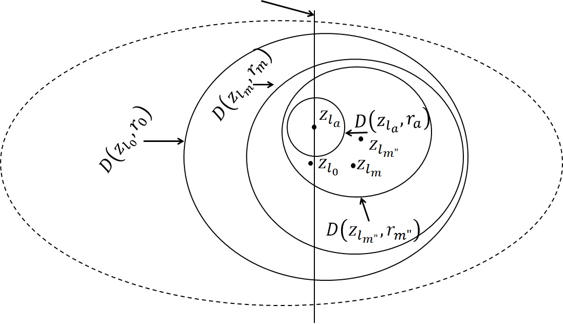
Figure 3.3. Nested discs and points on the intersection of planes.

∎

Remark 10.

As a consequence of Theorem 9, we will see that

$$\sum_{i=1}^{\infty}\int_{a_{0}^{l_{i}}}^{a_{0}^{l_{\infty}}}\left|z\left[v_{l_{i}}(\tau)\right]\right|v^{\prime}_{l_{i}}(\tau)d\tau\subset D\left(z_{l_{0}},r_{0}\right).$$

The random fluctuations and transitions explained in this sub-section could arise infinitely many times during $[t_{0},\infty).$ The random environment created on $\mathbb{C}_{l}$ and its behavior at the intersection of $\mathbb{C}_{l}$ and $\mathbb{C}_{0}$ is crucial for the creation of multilevel contours. A contour $\gamma_{l}$ could remain forever in $\mathbb{C}_{l}$ or could go beyond $\mathbb{C}_{l}$ and reach other planes. Contour $\gamma_{l}$ also has the potential to reach infinitely many planes and also has the potential to return to each and every plane infinitely many times.

Theorem 11.

There exists a unique contour $\gamma_{l}$ for each initial number chosen on $\mathbb{C}_{l}$ for $\mathbb{C}_{l}$ in the bundle $B_{\mathbb{R}}(\mathbb{C})$ combined with the $\mathbb{C}_{0}$ intersecting with the bundle and satisfying the property (7).

Proof.

Let $\gamma_{l}$ be a contour described by $z_{l}(t)$ for $t\in[t_{0},\infty)$ that has a starting point on the plane $\mathbb{C}_{l}$ with $z_{l}(t_{0})=z_{l_{0}}$ (say). The values of $z_{l}(t)$ can reach other planes because the bundle $B_{\mathbb{R}}(\mathbb{C})$ in which $\mathbb{C}_{l}$ lies is intersecting with the $\mathbb{C}_{0}.$ Due to the property (7), $X\left(z_{l}(t),\mathbb{C}_{l}\right)$ keeps on generating new numbers during $[t_{0},\infty)$ and $z_{l_{a}}\neq z_{l_{b}}$ for $a\neq b$ and $a,b\in\mathbb{R}.$ At some of time $\gamma_{l}$ could become a multilevel contour if the value generated by $X\left(z_{l}(t),\mathbb{C}_{l}\right)$ reaches another plane, say $\mathbb{C}_{p}$ for $\mathbb{C}_{p}\neq\mathbb{C}_{l}$. Reaching of another plane is possible due to the positioning of $\mathbb{C}_{0}.$ Or $\gamma_{l}$ could remain as a contour on $\mathbb{C}_{l}$ for $t\in[t_{0},\infty).$

In Theorem (8), we saw that a contour drawn from an initial number $z_{l_{0}}$ reaches $z_{l_{n}}$only through distinct numbers $z_{l_{1}},$ $z_{l_{2}},$ $...,z_{l_{n-1}}.$ The numbers $z_{l_{1}},$ $z_{l_{2}},$ $...,z_{l_{n-1}}$ were generated by $X\left(z_{l}(t),\mathbb{C}_{l}\right)$ . Alternatively, suppose the initial value chosen by $X\left(z_{l}(t),\mathbb{C}_{l}\right)$ is say, $z^{\prime}_{l_{0}}$ for $z^{\prime}_{l_{0}}\neq z_{l_{0}},$then even if the numbers $z_{l_{1}},$ $z_{l_{2}},$ $...,z_{l_{n-1}}$ are the same through which a contour up to $z_{l_{n}}$is drawn (due to the randomness in selection of complex numbers by $X\left(z_{l}(t),\mathbb{C}_{l}\right)$), a contour drawn from $z_{l_{0}}$to $z_{l_{n}}$ would be different than $z^{\prime}_{l_{0}}.$ This argument is valid for $\gamma_{l}$ a contour on $\mathbb{C}_{l}$ or a multilevel contour. Hence, as $t_{n}\rightarrow\infty$ the numbers generated by $X\left(z_{l}(t),\mathbb{C}_{l}\right)$ would be distinct due to the property (7). Therefore $\gamma_{l}$ is unique. ∎

Each point (number) on $\mathbb{C}_{l}$ has potentially capable to produce a contour which could remain forever in $\mathbb{C}_{l}$ or could become a multilevel contour by crossing $\mathbb{C}_{l}$ through $\mathbb{C}_{0}.$$X\left(z_{l}(t),\mathbb{C}_{l}\right)$ has the power to choose the first number of $\mathbb{C}_{l}$and generate rest of the numbers randomly. Due to the property (7), $X\left(z_{l}(t),\mathbb{C}_{l}\right)$ looses the power to choose a number that was already been chosen earlier. That is

$$p(z_{l_{a}},z_{l_{a}},t)\text{ }(t\in[t_{0},\infty))=0$$

where $p(z_{l_{a}},z_{l_{a}},t)$ is the probability of transition to the same number is zero. Suppose $z_{l_{0}},$ $z_{l_{1}}$, $z_{l_{2}},...,z_{l_{n}},...$ are the set of numbers generated by $X\left(z_{l}(t),\mathbb{C}_{l}\right)$ over the time. Let $p(z_{l_{0}},z_{l_{1}},t)^{(1)}$ represent the probability of reaching $z_{l_{1}}$from $z_{l_{0}}$in $1-$time interval $[t_{0},t_{1}]$, $p(z_{l_{0}},z_{l_{1}},t)^{(2)}$ represent the probability of reaching $z_{l_{2}}$from $z_{l_{0}}$in $2-$time intervals $[t_{0},t_{1}]$, $(t_{1},t_{2}]$, and so on. We note that $z_{l_{2}}$cannot be reached directly from $z_{l_{0}}$ in $1-$time interval $[t_{0},t_{1}]$ or $[t_{0},t_{2}]$ as mentioned previously in the article. So

(3.15) $$p(z_{l_{0}},z_{l_{2}},t)^{(2)}>0\text{ and }p(z_{l_{0}},z_{l_{2}},t)^{(1)}=0,$$

and

(3.16) $$p(z_{l_{1}},z_{l_{3}},t)^{(2)}>0\text{ and }p(z_{l_{1}},z_{l_{3}},t)^{(m)}=0,\text{ for }m=1,3,4,5,...$$

The $n-$time intervals transition probabilities between any other two distinct complex numbers on $\mathbb{C}_{l}$ can be expressed as in (3.15) and (3.16).

Remark 12.

The notation $X\left(z_{l}(t),\mathbb{C}_{l}\right)$ $t\in[t_{0},\infty)$ is used even if $X\left(z_{l}(t),\mathbb{C}_{l}\right)$ starts generating numbers from different plane after crossing through $\mathbb{C}_{0}$ after the initial value $z_{l_{0}}$ was chosen in $\mathbb{C}_{l}.$ Such notation will help identify the origin plane of $X\left(z_{l}(t),\mathbb{C}_{l}\right).$

Theorem 13.

Given $X\left(z_{l}(t_{0}),\mathbb{C}_{l}\right)=z_{l_{0}}.$ Suppose $p(z_{l_{a}},z_{l_{b}},t)^{(n)}$ represent $n-$time intervals transition probabilities from $z_{l_{a}}$to $z_{l_{b}}$ where

$$X\left(z_{l}(t),\mathbb{C}_{l}\right)=z_{l_{a}} \text{ for }t\in(t_{a-1},t_{a}]\,\text{and}$$

$$X\left(z_{l}(t),\mathbb{C}_{l}\right)=z_{l_{b}} \text{ for }t\in(t_{b-1},t_{b}],$$

for $t_{b}>t_{a}$, then

$$p(z_{l_{a}},z_{l_{b}},t)^{(n)}=\left\{\begin{array}[]{c}>0\text{ if }n=t_{b}-t_{a\text{ }}\text{ sequential time intervals}\\ =0\text{ if }n\neq t_{b}-t_{a}\text{ sequential time intervals}\end{array}\right..$$

Proof.

The $n-$time interval transition probability $p(z_{l_{a}},z_{l_{b}},t)^{(n)}$ is written as

$$p(z_{l}(t_{a}),z_{l}(t_{b}),t)^{(n)}\text{ }\left(t\in(t_{a},t_{b}]\right) =p(z_{l_{a}},z_{l_{a_{1}}},t)^{(1)}\text{ }\left(t\in(t_{a},t_{a_{1}}]\right).$$

$$p(z_{l_{a_{1}}},z_{l_{a_{2}}},t)^{(1)}\text{ }\left(t\in(t_{a_{1}},t_{a_{2}}]\right).$$

(3.17) $$....p(z_{l_{a_{n-1}}},z_{l_{b}},t)^{(1)}\text{ }\left(t\in(t_{a_{n-1}},t_{b}]\right),$$

for $t_{a}<t_{a_{1}}<...t_{a_{n-1}}<t_{b}.$ In (3.17), $z_{l_{a_{1}}}$ is generated by $X\left(z_{l}(t),\mathbb{C}_{l}\right)$ during $(t_{a},t_{a_{1}}]$ from the set of numbers of the disc $D(z_{l_{a}},r_{a})$, $z_{l_{a_{2}}}$ is generated by $X\left(z_{l}(t),\mathbb{C}_{l}\right)$ during $(t_{a_{1}},t_{a_{2}}]$ from the set of numbers of the disc $D(z_{l_{a_{1}}},r_{a_{1}})$, and so on, $z_{l_{b}}$ is generated by $X\left(z_{l}(t),\mathbb{C}_{l}\right)$ during $(t_{a_{n-1}},t_{b}]$ from the set of numbers of the disc $D(z_{l_{a_{n-1}}},r_{a_{n-1}}).$ The numbers $z_{l_{a_{1}}},$ $z_{l_{a_{2}}}$, $...,$ $z_{l_{a_{n-1}}}$, $z_{l_{b}}$were sequentially generated from the sets of distinct discs

(3.18) $$\left\{D(z_{l_{a}},r_{a}),D(z_{l_{a_{1}}},r_{a_{1}}),...,D(z_{l_{a_{n-1}}},r_{a_{n-1}})\right\}$$

within the sequential time intervals

(3.19) $$\left\{(t_{a},t_{a_{1}}],(t_{a_{1}},t_{a_{2}}],...,(t_{a_{n-1}},t_{b}]\right\}$$

Due to the sequential nature of (3.18) and (3.19), we will have

$$p(z_{l_{a}},z_{l_{a_{1}}},t)^{(1)}\text{ }\left(t\in(t_{a},t_{a_{1}}]\right) >0$$

$$p(z_{l_{a_{1}}},z_{l_{a_{2}}},t)^{(1)}\text{ }\left(t\in(t_{a_{1}},t_{a_{2}}]\right) >0$$

$$\vdots$$

(3.20) $$p(z_{l_{a_{n-1}}},z_{l_{b}},t)^{(1)}\text{ }\left(t\in(t_{a_{n-1}},t_{b}]\right) >0.$$

From (3.20) we conclude that

(3.21) $$p(z_{l}(t_{a}),z_{l}(t_{b}),t)^{(n)}\text{ }\left(t\in(t_{a},t_{b}]\right)>0.$$

We also note that,

$$t_{a_{1}-t_{a}} =1-\text{ step time interval}$$

$$t_{a_{2}-t_{a_{1}}} =1-\text{ step time interval}$$

$$\vdots$$

(3.22) $$t_{b}-t_{a_{n-1}} =1-\text{ step time interval}$$

Summing up the terms of the L.H.S. of (3.22) and equating it to sum of the quantities of the R.H.S. of (3.22), we see that

(3.23) $$t_{b}-t_{a}=n-\text{ sequential time intervals}.$$

From (3.21) and (3.23) we conclude that $p(z_{l_{a}},z_{l_{b}},t)^{(n)}>0$ when $t_{b}-t_{a}=n-\text{ sequential time intervals}.$

Suppose $t_{b}-t_{a}\neq m-\text{ sequential time intervals}.$ This implies $z_{l_{b}}$is generated either through less than $m-$ sequential time intervals after choosing $z_{l_{a}}$ by $X\left(z_{l}(t),\mathbb{C}_{l}\right)$ or $z_{l_{b}}$is generated through more than $m-$ sequential time intervals after choosing $z_{l_{a}}$ by $X\left(z_{l}(t),\mathbb{C}_{l}\right).$ If $m=1,$then

$$t_{b}-t_{a}\neq 1,\text{which implies,}p(z_{l_{a}},z_{l_{b}},t)^{(1)}=0$$

if $m=2,$then

$$t_{b}-t_{a}\neq 2,\text{which implies,}p(z_{l_{a}},z_{l_{b}},t)^{(2)}=0$$

and so on if $m=n,$then

$$t_{b}-t_{a}\neq n,\text{which implies,}p(z_{l_{a}},z_{l_{b}},t)^{(n)}=0.$$

This concludes that $p(z_{l_{a}},z_{l_{b}},t)^{(n)}=0$ if $n\neq t_{b}-t_{a}\text{ sequential time intervals}.$

Each number in $\mathbb{C}_{l}$ that was chosen initially by $X\left(z_{l}(t),\mathbb{C}_{l}\right)$ and further points chosen by $X\left(z_{l}(t),\mathbb{C}_{l}\right)$ over the time $[t_{0},\infty)$ forms the state space of $X\left(z_{l}(t),\mathbb{C}_{l}\right)$ and is given by

$$A_{X}(\mathbb{C}_{l})= \left\{z:z=z_{l_{0}}\text{ at }X\left(z_{l}(t_{0}),\mathbb{C}_{l}\right)\text{ and $X\left(z_{l}(t),\mathbb{C}_{l}\right)\left(t_{0},\infty\right)=z$ }\right.$$

for z$$\in B_{\mathbb{R}} \mathbb{C}$$().

$$\text{Here the order of choosing }z\text{ is preserved and }z_{l_{a}}\neq z_{l_{b}}$$

$$\left.\text{ if }a\neq b,\text{ }a,b>t_{0}\right\}$$

As the time progresses it will keep on reaching new numbers in $B_{\mathbb{R}}(\mathbb{C}).$ All the elements of the set $A_{X}(\mathbb{C}_{l})$ need not be in $\mathbb{C}_{l}$ due to behavior of $X\left(z_{l}(t_{0}),\mathbb{C}_{l}\right)$ at $\mathbb{C}_{l}\cap\mathbb{C}_{0}$ explained previously. The points of $A_{X}(\mathbb{C}_{l})$ could be forever in $\mathbb{C}_{l}$ or they could spread across one or more planes of $B_{\mathbb{R}}(\mathbb{C}).$ Each element in $A_{X}(\mathbb{C}_{l})$ is called a state of the process $\left\{X\left(z_{l}(t),\mathbb{C}_{l}\right)\right\}_{t\geq t_{0}}.$ If there is no certainty to return to a state after leave that state by the random variable, we call it a transient state. In this case, once $X\left(z_{l}(t),\mathbb{C}_{l}\right)$ chooses a state then it won’t be able to return to that state forever. Since there is an equal probability for $X\left(z_{l}(t),\mathbb{C}_{l}\right)$ to choose any complex number on $\mathbb{C}_{l}$, so there is a possibility to form contours of infinite lengths starting from each point on plane $\mathbb{C}_{l}.$ However, these infinite lengths of contours need not be identical. Suppose we define another process $\left\{Y\left(z_{l}(t),\mathbb{C}_{l}\right)\right\}_{t\geq t_{0}}$ with a two-step randomness that we used for generating the discs and radii then we consider these two processes $\left\{X\left(z_{l}(t),\mathbb{C}_{l}\right)\right\}_{t\geq t_{0}}$ and $\left\{X\left(z_{l}(t),\mathbb{C}_{l}\right)\right\}_{t\geq t_{0}}$ are not disjoint to each other, that is, both these processes have some probability to choose identical values in the same order or in different order during $[t_{0},\infty).$ ∎

Theorem 14.

Two contours formed during $[t_{0},\infty)$ need not be identical but their lengths could be identical.

Proof.

Let $\gamma_{l}(X)$ and $\gamma_{l}(Y)$ be two contours formed out of the points created by two processes $\left\{X\left(z_{l}(t),\mathbb{C}_{l}\right)\right\}_{t\geq t_{0}}$ and $\left\{Y\left(z_{l}(t),\mathbb{C}_{l}\right)\right\}_{t\geq t_{0}}$ with $\left\{X\left(z_{l}(t_{0}),\mathbb{C}_{l}\right)\right\}=z_{l_{0}}(X)$ and $\left\{Y\left(z_{l}(t_{0}),\mathbb{C}_{l}\right)\right\}=z_{l_{0}}(Y).$ Let $\gamma_{l}(X)$ be described by $z_{X}(t)$ $[t_{0},\infty)$ and $\gamma_{l}(Y)$ be described by $z_{Y}(t)$ $[t_{0},\infty)$. The two state spaces corresponding to the two processes are

$$A_{X}(\mathbb{C}_{l}) =\left\{z:z=z_{l_{0}}(X)\text{ at }X\left(z_{l}(t_{0}),\mathbb{C}_{l}\right)\text{ and $X\left(z_{l}(t),\mathbb{C}_{l}\right)\left(t_{0},\infty\right)=z$ }\right.$$

$$\text{for }z\in B_{\mathbb{R}}(\mathbb{C})$$

$$\text{with some order of choosing }z\text{ and }z_{l_{a}}(X)\neq z_{l_{b}}(X)$$

$$\left.\text{ if }a\neq b,\text{ }a,b>t_{0}\right\}$$

$$A_{Y}(\mathbb{C}_{l}) =\left\{z:z=z_{l_{0}}(Y)\text{ at }Y\left(z_{l}(t_{0}),\mathbb{C}_{l}\right)\text{ and $Y\left(z_{l}(t),\mathbb{C}_{l}\right)\left(t_{0},\infty\right)=z$ }\right.$$

for z$$\in B_{\mathbb{R}} \mathbb{C}$$().

$$\text{with some order of choosing }z\text{ and }z_{l_{a}}(Y)\neq z_{l_{b}}(Y)$$

$$\left.\text{ if }a\neq b,\text{ }a,b>t_{0}\right\}$$

Note, $\gamma_{l}(X)$ is identical to $\gamma_{l}(Y)$ if, and only if, $z_{l_{0}}(X)=z_{l_{0}}(Y)$ and all other $z$ values generated out of infinite iterations of two processes are identical, i.e. $A_{X}(\mathbb{C}_{l})=A_{Y}(\mathbb{C}_{l})$. Since $A_{X}(\mathbb{C}_{l})$ and $A_{Y}(\mathbb{C}_{l})$ are not disjoint, there is a possibility that $\left\{X\left(z_{l}(t),\mathbb{C}_{l}\right)\right\}_{t\geq t_{0}}$ and $\left\{Y\left(z_{l}(t),\mathbb{C}_{l}\right)\right\}_{t\geq t_{0}}$ may choose same numbers during $[t_{0},\infty).$ If $A_{X}(\mathbb{C}_{l})\neq A_{Y}(\mathbb{C}_{l})$, then anyway $\gamma_{l}(X)$ is not identical to $\gamma_{l}(Y).$ Given that $A_{X}(\mathbb{C}_{l})$ and $A_{Y}(\mathbb{C}_{l})$ are available, let $L\left[(z_{l_{0}}(X),z_{l_{a}}(X)\right]$ be the length of the contour from $z_{l_{0}}(X)$ to $z_{l_{a}}(X)$ and $L\left[(z_{l_{a}}(X),z_{l_{b}}(X)\right]$ be the length of the contour from $z_{l_{a}}(X)$ to $z_{l_{b}}(X)$ such that the length of the contour from $z_{l_{0}}(X)$ to $z_{l_{a}}(X)$ is computed as

(3.24) $$L\left[(z_{l_{0}}(X),z_{l_{b}}(X)\right]=L\left[(z_{l_{0}}(X),z_{l_{a}}(X)\right]+L\left[(z_{l_{a}}(X),z_{l_{b}}(X)\right].$$

Let $L\left[(z_{l_{0}}(Y),z_{l_{a}}(Y)\right]$ be the length of the contour from $z_{l_{0}}(Y)$ to $z_{l_{a}}(Y)$ and $L\left[(z_{l_{a}}(Y),z_{l_{b}}(Y)\right]$ be the length of the contour from $z_{l_{a}}(Y)$ to $z_{l_{b}}(Y)$ such that the length of the contour from $z_{l_{0}}(Y)$ to $z_{l_{a}}(Y)$ is computed as

(3.25) $$L\left[(z_{l_{0}}(Y),z_{l_{b}}(Y)\right]=L\left[(z_{l_{0}}(Y),z_{l_{a}}(Y)\right]+L\left[(z_{l_{a}}(Y),z_{l_{b}}(Y)\right].$$

In (3.24) and (3.25), it is assumed that $z_{l_{0}}(X)\neq z_{l_{0}}(Y)$, $z_{l_{a}}(X)\neq z_{l_{a}}(X)$, and $z_{l_{b}}(X)\neq z_{l_{b}}(Y).$ Suppose

$$L\left[(z_{l_{0}}(X),z_{l_{a}}(X)\right]\neq L\left[(z_{l_{0}}(Y),z_{l_{a}}(Y)\right]\text{ and }$$

$$L\left[(z_{l_{0}}(X),z_{l_{a}}(X)\right]<L\left[(z_{l_{0}}(Y),z_{l_{a}}(Y)\right]$$

and

$$L\left[(z_{l_{a}}(X),z_{l_{b}}(X)\right]\neq L\left[(z_{l_{a}}(Y),z_{l_{b}}(Y)\right]\text{ and }$$

$$L\left[(z_{l_{a}}(X),z_{l_{b}}(X)\right]>L\left[(z_{l_{a}}(Y),z_{l_{b}}(Y)\right]$$

such that

$$L\left[(z_{l_{0}}(Y),z_{l_{a}}(Y)\right]-L\left[(z_{l_{0}}(X),z_{l_{a}}(X)\right] =$$

(3.26) $$L\left[(z_{l_{a}}(X),z_{l_{b}}(X)\right]-L\left[(z_{l_{a}}(Y),z_{l_{b}}(Y)\right]$$

By (3.26), we conclude that $L\left[(z_{l_{0}}(X),z_{l_{b}}(X)\right]=L\left[(z_{l_{0}}(Y),z_{l_{b}}(Y)\right].$ Since $t_{a}$ and $t_{b}$ are arbitrary, one can extend the result to other contour distances. ∎

Theorem 15.

Two state spaces $A_{X}(\mathbb{C}_{l})$ and $A_{Y}(\mathbb{C}_{l})$ are identical need not imply the corresponding contours are identical.

Proof.

Given that the two state spaces $A_{X}(\mathbb{C}_{l})$ and $A_{Y}(\mathbb{C}_{l})$ are identical. This implies the states in $A_{X}(\mathbb{C}_{l})$ and $A_{Y}(\mathbb{C}_{l})$ are the same. Suppose the order of the states generated by $\left\{X\left(z_{l}(t),\mathbb{C}_{l}\right)\right\}_{t\geq t_{0}}$ and $\left\{Y\left(z_{l}(t),\mathbb{C}_{l}\right)\right\}_{t\geq t_{0}}$ are the same, then the two contours $\gamma_{l}(X)$ and $\gamma_{l}(Y)$ are identical.

Suppose $z_{l_{0}}(X)=z_{l_{0}}(Y)$ but the randomness has resulted in distinct order of the states in $A_{X}(\mathbb{C}_{l})$ and $A_{Y}(\mathbb{C}_{l})$ such that

$$z_{l_{a}}(X)=z_{l_{b}}(Y)\text{ and }z_{l_{b}}(X)=z_{l_{a}}(Y)$$

for some arbitrary $t_{a}$ and $t_{b}.$ This implies $\gamma_{l}(X)$ be no more identical to $\gamma_{l}(Y).$ ∎

The length of a contour is less sensitive for fluctuations due to randomness than the contour itself. When $z_{l_{0}}(X)\neq z_{l_{0}}(Y),$ then $\gamma_{l}(X)\neq\gamma_{l}(Y)$ but in the long run, say for some $t$ $(T,\infty)$, the lengths of $\gamma_{l}(X)$ and $\gamma_{l}(Y)$ could be the same. Once $A_{X}(\mathbb{C}_{l})$ and $A_{Y}(\mathbb{C}_{l})$ are formed by the two non-disjoint processes $\left\{X\left(z_{l}(t),\mathbb{C}_{l}\right)\right\}_{t\geq t_{0}}$ and $\left\{Y\left(z_{l}(t),\mathbb{C}_{l}\right)\right\}_{t\geq t_{0}}$, then

$$p\left(z_{l_{0}}(X),z_{l_{0}}(X),t\right)^{(n)}\left(t\in[t_{0},\infty)\right)=0\text{ for }n=1,2,...$$

$$p\left(z_{l_{0}}(Y),z_{l_{0}}(Y),t\right)^{(n)}\left(t\in[t_{0},\infty)\right)=0\text{ for }n=1,2,...$$

and

$$p\left(z_{l_{a}}(X),z_{l_{a}}(X),t\right)^{(n)}\left(t\in[t_{0},\infty)\right)=0\text{ for }n=1,2,...$$

for an arbitrary $z_{l_{a}}(X)$ chosen by $X\left(z_{l}(t),\mathbb{C}_{l}\right)$,

$$p\left(z_{l_{a}}(Y),z_{l_{a}}(Y),t\right)^{(n)}\left(t\in[t_{0},\infty)\right)=0\text{ for }n=1,2,...$$

for an arbitrary $z_{l_{a}}(Y)$ chosen by $Y\left(z_{l}(t),\mathbb{C}_{l}\right)$. These imply,

$$\sum_{n=1}^{\infty}p\left(z_{l_{a}}(X),z_{l_{a}}(X),t\right)^{(n)}\left(t\in[t_{0},\infty)\right)=0$$

$$\sum_{n=1}^{\infty}p\left(z_{l_{a}}(Y),z_{l_{a}}(Y),t\right)^{(n)}\left(t\in[t_{0},\infty)\right)=0.$$

Suppose the real valued function $v_{l}(X,\tau)$ maps $[a_{0}^{l},\infty)$ onto the interval $[t_{0},\infty)$, then

$$L(\gamma_{l},X) =\int_{a_{0}^{l}}^{\infty}\left|z\left[v_{l}(X,\tau)\right]\right|v^{\prime}_{l}(X,\tau)d\tau$$

$$=\int_{a_{0}^{l}}^{\infty}\left|z\left[v_{l}(Y,\tau)\right]\right|v^{\prime}_{l}(Y,\tau)d\tau$$

$$=L(\gamma_{l},Y)$$

where  the real valued function $v_{l}(Y,\tau)$ maps $[a_{0}^{l},\infty)$ onto the interval $[t_{0},\infty)$. Only looking at the integral expressions used for $L(\gamma_{l},X)$ or $L(\gamma_{l},Y)$, we are unable to tell about whether a contour $\gamma_{l}(X)$ has traveled to any other planes beyond $\mathbb{C}_{l}.$ The symbol $l$ in $\gamma_{l}(X)$ stands for the plane from which this contour has originated and $X$ stands $X\left(z_{l}(t),\mathbb{C}_{l}\right)$ indicates the random variable responsible for generating data required to form $\gamma_{l}(X).$ Suppose we consider infinitely many random variables of the type $X\left(z_{l}(t),\mathbb{C}_{l}\right)$ to satisfy two conditions, $(i).$ Each of these works non-disjointly such that they may choose an initial value that was chosen by a different random variable, and $(ii).$ Each of these random variables chooses an initial value that is distinct from others such that the number of initial values is again the number of random variables. Let $\alpha$ be the number of distinct initial values satisfying the condition $(i)$ such that $\alpha$ is less than the cardinality of $\mathbb{C}_{l}$ and let $X^{\prime}$ be the index random variable. Then the total lengths of all the contours originated by all the random variables of condition $(i)$ is

(3.27) $$L(\gamma_{l},X^{\prime},\alpha)=\sum_{\alpha}\int_{a_{0}^{l}}^{\infty}\left|z\left[v_{l}(X^{\prime},\alpha,\tau)\right]\right|v^{\prime}_{l}(X^{\prime},\alpha,\tau)d\tau d\alpha$$

Let $\beta$ be the distinct initial values in the condition $(ii)$ due to distinct random variables within the condition $(ii)$ with a then the total length of all the contours generated due to condition $(ii)$ is

(3.28) $$L(\gamma_{l},X^{\prime},\beta)=\sum_{\beta}\int_{a_{0}^{l}}^{\infty}\left|z\left[v_{l}(X^{\prime},\beta,\tau)\right]\right|v^{\prime}_{l}(X^{\prime},\alpha,\tau)d\tau d\beta.$$

There is no comparative measure between (3.27) and (3.28), but

$$L(\gamma_{l},X^{\prime},\alpha) \subset B_{\mathbb{R}}(\mathbb{C}),$$

$$L(\gamma_{l},X^{\prime},\beta) \subset B_{\mathbb{R}}(\mathbb{C}).$$

and

$$L(\gamma_{l},X^{\prime},\alpha) \subset\bigcup_{\alpha}\bigcup_{z_{l_{a}}\in\mathbb{C}_{l}}D(z_{l_{a}},r_{a},X^{\prime},\alpha)$$

$$L(\gamma_{l},X^{\prime},\beta) \subset\bigcup_{\beta}\bigcup_{z_{l_{a}}\in\mathbb{C}_{l}}D(z_{l_{a}},r_{a},X^{\prime},\beta)$$

where $D(z_{l_{a}},r_{a},X^{\prime},\alpha)$ and $D(z_{l_{a}},r_{a},X^{\prime},\alpha)$ represent discs generated through two-step randomness for conditions $(i)$ and $(ii).$The procedure for generating these discs remains the same as described previously. Currently, we have not considered the spaces created due to overlapping contours by these infinitely many contours generated due to conditions $(i)$ and $(ii).$ However,

$$\bigcup_{\alpha}\bigcup_{z_{l_{a}}\in\mathbb{C}_{l}}D(z_{l_{a}},r_{a},X^{\prime},\alpha)\neq\bigcup_{\beta}\bigcup_{z_{l_{a}}\in\mathbb{C}_{l}}D(z_{l_{a}},r_{a},X^{\prime},\beta)$$

if the origins of contours created in $(i)$ and $(ii)$ are different.

Theorem 16.

Suppose infinitely many random variables of the type $X\left(z_{l}(t),\mathbb{C}_{l}\right)$ are available whose cardinality is same as that of $\mathbb{C}_{l}$ and two different conditions $(i)$ and $(ii)$ above are given. The union of the sets of discs formed under these two conditions could be different or the same.

Proof.

Let us consider infinitely many random variables within the condition $(i).$ Let the arbitrary variable be $X^{\prime}\left(z_{l}(t),\mathbb{C}_{l},\alpha\right)\text{}\left(t\in[t_{0},\infty\right)$ for $\alpha$ as in condition $(i)$ described above. Let $X^{\prime}\left(z_{l}(t),\mathbb{C}_{l},\alpha\right)=z_{l_{0}}(t_{0},X^{\prime},\alpha).$ The set of discs formed due to each $X^{\prime}\left(z_{l}(t),\mathbb{C}_{l},\alpha\right)$ are infinite. Each point on the plane could be the origin of a contour on $\mathbb{C}_{l}.$ This imply, there is a possibility that

(3.29) $$\bigcup_{z_{l_{a}}\in\mathbb{C}_{l}}D(z_{l_{0}},r_{0},X^{\prime},\alpha)=\bigcup_{z_{l_{a}}\in\mathbb{C}_{l}}D(z_{l_{0}},r_{0},X^{\prime},\beta)$$

Note that $r_{0}$ is associated with two step randomness of each $X^{\prime}\left(z_{l}(t),\mathbb{C}_{l},\alpha\right)$ and $r_{0}$values are generated separately for conditions $(i)$ and $(ii).$ So, $r_{0}$ in the L.H.S. of (3.29) need not be equal to the $r_{0}$ of R.H.S of (3.29). When randomly each $X^{\prime}\left(z_{l}(t),\mathbb{C}_{l},\alpha\right)$ chooses different origins and $r_{0}$s of each $z_{l_{0}}(t_{0},X^{\prime},\alpha)$ corresponding to each $X^{\prime}\left(z_{l}(t),\mathbb{C}_{l},\alpha\right)$ are identical then (3.29) holds. If these $r_{0}s$ are different then (3.29) does not hold. Once (3.29) holds, then suppose the $r_{a}$s for $z_{l_{a}}(t_{a},X^{\prime},\alpha)$ corresponding to each $X^{\prime}\left(z_{l}(t),\mathbb{C}_{l},\alpha\right)$ are identical to the $r_{a}$s for $z_{l_{a}}(t_{a},X^{\prime},\beta)$ corresponding to each $X^{\prime}\left(z_{l}(t),\mathbb{C}_{l},\beta\right)$ for each of the infinitely many time intervals, then

$$\bigcup_{\alpha}\bigcup_{z_{l_{a}}\in\mathbb{C}_{l}}D(z_{l_{a}},r_{a},X^{\prime},\alpha)=\bigcup_{\beta}\bigcup_{z_{l_{a}}\in\mathbb{C}_{l}}D(z_{l_{a}},r_{a},X^{\prime},\beta),$$

else, if at least one such $r_{a}$ that was chosen randomly is different in conditions $(i)$ and $(ii)$ then

$$\bigcup_{\alpha}\bigcup_{z_{l_{a}}\in\mathbb{C}_{l}}D(z_{l_{a}},r_{a},X^{\prime},\alpha)\neq\bigcup_{\beta}\bigcup_{z_{l_{a}}\in\mathbb{C}_{l}}D(z_{l_{a}},r_{a},X^{\prime},\beta).$$

∎

We have

$$\bigcup_{\beta}\bigcup_{z_{l_{a}}\in\mathbb{C}_{l}}D(z_{l_{a}},r_{a},X^{\prime},\beta)=\mathbb{C}_{l}$$

because $z_{l_{a}}\in\bigcup_{\beta}\bigcup_{z_{l_{a}}\in\mathbb{C}_{l}}D(z_{l_{a}},r_{a},X^{\prime},\beta)$ implies $z_{l_{a}}\in\mathbb{C}_{l}$ for each $z_{l_{a}}$ and $z_{l_{a}}\in\mathbb{C}_{l}$ implies $z_{l_{a}}\in\bigcup_{\beta}\bigcup_{z_{l_{a}}\in\mathbb{C}_{l}}D(z_{l_{a}},r_{a},X^{\prime},\beta).$ For condition $(ii)$ within every disc, there are infinitely many points of other contours. Whereas, such an assertion is not possible for the discs generated under the condition $(ii).$ There is no chance to form an isolated disc under the two step randomness procedure and Markov property derived earlier still holds for the discs formed under these two conditions. For a general description of continuous-time Markov property, refer, for example to [6, 7, 8, 9, 10].

Remark 17.

Under random environment the possibility for having identical $r_{a}$ values in each iteration of $X^{\prime}\left(z_{l}(t),\mathbb{C}_{l},\alpha\right)$ for infinitely many time interval is very small. So the chances for below equality can be treated as a rare event:

$$D(z_{l_{a}},r_{a},X^{\prime},\alpha) =D(z_{l_{a}},r_{a},X^{\prime},\beta)\text{ for }t\in(t_{a},t_{a^{\prime}}]$$

$$D(z_{l_{a^{\prime}}},r_{a^{\prime}},X^{\prime},\alpha) =D(z_{l_{a^{\prime}}},r_{a^{\prime}},X^{\prime},\beta)\text{ for }t\in(t_{a^{\prime}},t_{a^{\prime\prime}}]$$

$$\vdots \vdots$$

$$D(z_{l_{b}},r_{b},X^{\prime},\alpha) =D(z_{l_{b}},r_{b},X^{\prime},\beta)\text{ for }t\in(t_{b},t_{b}]$$

$$\vdots \vdots$$

Remark 18.

When we relax the assumption in (3.3) and (7) for the possibility to choose the same state by $X\left(z_{l}(t),\mathbb{C}_{l}\right)$ after that state has been chosen earlier by $X\left(z_{l}(t),\mathbb{C}_{l}\right)$, then each state in $A_{X}(\mathbb{C}_{l})$ becomes recurrent. For a recurrent state, the probability to return to a state is certain even if it takes a very large number of time intervals. We can draw many contours like $\gamma_{l}(X)$, $\gamma_{l}(Y)$, etc., Each contour will have its starting point or the origin depending upon the initial value chosen by the random variable responsible to generate the data required. A thick forest of contours can be formed from infinitely many random variables. A family of infinitely many random variables of type $X\left(z_{l}(t),\mathbb{C}_{l}\right)$ could form a forest of contours. Let this family be $\mathcal{F}_{l}$

$$\mathcal{F}_{l}=\left\{X\left(z_{l}(t),\mathbb{C}_{l}\right),Y\left(z_{l}(t),\mathbb{C}_{l}\right),...\right\}$$

for the set of random variables defined on $\mathbb{C}_{l}$. Let $\mathcal{F}_{l}$ satisfies (3.3) and (7). Each element within $\mathcal{F}_{l}$ will have infinitely many points called the state spaces. Each state space will have infinitely many states. A family $\mathcal{F}_{l}$ is recurrent if all the elements of $\mathcal{F}_{l}$ are recurrent and if not $\mathcal{F}_{l}$ is called transient. A transient family $\mathcal{F}_{l}$ would have a higher possibility to form a relatively quicker dense forest of contours than a recurrent family. These dense forests of contours could spread over one or more planes in bundle $B_{\mathbb{R}}(\mathbb{C})$.

3.2. Loss of Spaces in Bundle $B_{\mathbb{R}}(\mathbb{C})$

Suppose we continue our investigations of the behavior of $X\left(z_{l}(t),\mathbb{C}_{l}\right)$ with the properties of distinct complex numbers as described in Section 3.1. Let $\gamma_{l}(X,t)$ be the contour formed out of the set of points $z_{l}(t)$ $(t\in[t_{0},\infty))$ sequentially chosen as per two step randomness of $\left\{X\left(z_{l}(t),\mathbb{C}_{l}\right)\right\}_{t\geq t_{0}}$ and has origin in the plane $\mathbb{C}_{l}$. Suppose the space created by $\gamma_{l}(X,t)$ $(t\in[t_{0},\infty)$ is removed from $B_{\mathbb{R}}(\mathbb{C}).$ Let $[\gamma_{l}(X,t)]^{c}$ be the space of all points of the $B_{\mathbb{R}}(\mathbb{C})$ minus the points of the contour. Let us assume that $\gamma_{l}(X,t)$ is formed out of the distinct complex numbers described in the previous section. That is,

$$[\gamma_{l}(X,t)]^{c}=B_{\mathbb{R}}(\mathbb{C})\backslash\gamma_{l}(X,t)=\left\{z_{l}:z_{l}\in B_{\mathbb{R}}(\mathbb{C})\text{ and }z_{l}\notin\gamma_{l}(X,t)\right\}.$$

When we introduce another random variable $Y\left(z_{l}(t),\mathbb{C}_{l}\right),$ we assume that the space lost due to $\gamma_{l}(X,t)$ is not available for $Y\left(z_{l}(t),\mathbb{C}_{l}\right).$ That is, $Y\left(z_{l}(t),\mathbb{C}_{l}\right)$ can choose numbers out of $[\gamma_{l}(X,t)]^{c}.$ The two step randomness is flexible to choose a radius and the next number within a disc until a number is found. This implies $\gamma_{l}(Y,t)$ can be formed continuously without any obstructions from the available numbers of the bundle. The timing between introducing process $X\left(z_{l}(t),\mathbb{C}_{l}\right)$ and removing a set of data created by $\gamma_{l}(X,t)$ up to a certain time $t$ would form a removal process. The elements or numbers that the process $X\left(z_{l}(t),\mathbb{C}_{l}\right)$ occupies over a time interval will be nothing new and they are part of $B_{\mathbb{R}}(\mathbb{C}).$ Due to the removal of the data occupied by the contour $\gamma_{l}(X,t)$ during the time interval, say $[t_{0},t_{d_{1}}]$, the bundle has lost elements from it. Since $\left\{X\left(z_{l}(t),\mathbb{C}_{l}\right)\right\}_{t\geq t_{0}}$ is a continuous process, the contour $\gamma_{l}(Y,t)$ still be forming after removal process has started at $t_{d_{1}}.$ Suppose $\left\{X\left(z_{l}(t),\mathbb{C}_{l}\right)\right\}_{t\geq t_{0}}$ has generated discs for a long time intervals up to $t_{b}$ by the time removal process has started. Here $t_{b}>t_{d_{1}}.$ All the elements of the contour $\gamma_{l}(X,t)$ that was formed during $t_{0},t_{d_{1}}]$ are nothing but the elements on the c0ontout until $t_{d_{1}}$ whose length is

$$\int_{a_{0}^{l_{0}}}^{a_{0}^{l_{d_{1}}}}\left|z[v_{l_{d_{1}}}(\tau)]\right|v^{\prime}_{l_{d_{1}}}(\tau)d\tau$$

for a real-valued function $v_{l_{d_{1}}}$ mapping $[a_{0}^{l_{0}},a_{0}^{l_{d_{1}}}]$ onto the interval $[t_{0},t_{d_{1}}].$ The set of elements on this contour are the set $z_{l}(t)$ $(t\in[t_{0},t_{d_{1}}])$ and denoted by $\gamma_{l}(X,t)$ $(t\in[t_{0},t_{d_{1}}])$. The remaining elements in the bundle are

$$B_{\mathbb{R}}(\mathbb{C}) -\phi_{1}(X)B_{\mathbb{R}}(\mathbb{C})$$

where $$\phi_{1}(X)=\frac{\gamma_{l}(X,t)(t\in[t_{0},t_{d_{1}}])}{B_{\mathbb{R}}(\mathbb{C})}$$

and differential equation describing the dynamics is

$$\frac{dB_{\mathbb{R}}(\mathbb{C})}{dt}=B_{\mathbb{R}}(\mathbb{C})-\phi_{1}(X)B_{\mathbb{R}}(\mathbb{C})\text{ for (t$\in$[$t_{0}$,$t_{d_{1}}$])}.$$

Suppose we remove the elements of the contour $\gamma_{l}(X,t)$ that was formed during $(t_{d_{1}},t_{d_{2}}]$ from $B_{\mathbb{R}}(\mathbb{C})$ such that $t_{d_{2}}-t_{d_{1}}=t_{d_{1}}-t_{0}.$ The rate of change in the bundle $B_{\mathbb{R}}(\mathbb{C})\backslash\gamma_{l}(X,t)$ $(t\in[t_{0},t_{d_{1}}]$ during $(t_{d_{1}},t_{d_{2}}]$ is

$$\frac{dB_{\mathbb{R}}(\mathbb{C})}{dt}\mid_{t=t_{d_{1}}}=B_{\mathbb{R}}(\mathbb{C})\mid_{t=t_{d_{1}}}-\phi_{2}(X)B_{\mathbb{R}}(\mathbb{C})\mid_{t=t_{d_{1}}}\text{ for (t$\in$[$t_{d_{1}}$,$t_{d_{2}}$])}$$

where $B_{\mathbb{R}}(\mathbb{C})\mid_{t=t_{d_{1}}}$ indicates the space of $B_{\mathbb{R}}(\mathbb{C})$ that was available at $t=t_{d_{1}}$and

$$\phi_{2}(X)=\frac{\gamma_{l}(X,t)(t\in[t_{d_{1}},t_{d_{2}}])}{B_{\mathbb{R}}(\mathbb{C})\mid_{t=t_{d_{1}}}}.$$

Suppose $t_{d_{1}}$ is randomly chosen, and the rest of all the time intervals are fixed to maintain the interval lengths equal to $t_{d_{1}}-t_{0}.$ The time intervals have constant length but the piecewise contour lengths in these intervals need not be identical because the contour formation is dependent on two step randomness and corresponding discs formations. The process of removal continues after $t_{d_{1}}$and $\phi$ be the rate of removal of elements from $B_{\mathbb{R}}(\mathbb{C})$, then this can be expressed with a differential equation

(3.30) $$\frac{dB_{\mathbb{R}}(\mathbb{C})}{dt}=B_{\mathbb{R}}(\mathbb{C})-\phi(X)B_{\mathbb{R}}(\mathbb{C}).$$

A constant rate of removal of elements is difficult to imagine because within the each time intervals

$$\left\{[t_{0},t_{d_{1}}],(t_{d_{1}},t_{d_{2}}],...\right\}$$

the number of elements to be removed depends on the lengths of contour formed during these intervals. These contour lengths are

$$\int_{a_{0}^{l_{d_{1}}}}^{a_{0}^{l_{d_{2}}}}\left|z[v_{l_{d_{2}}}(\tau)]\right|v^{\prime}_{l_{d_{2}}}(\tau)d\tau,$$

(3.31) $$\int_{a_{0}^{l_{d_{2}}}}^{a_{0}^{l_{d_{3}}}}\left|z[v_{l_{d_{3}}}(\tau)]\right|v^{\prime}_{l_{d_{3}}}(\tau)d\tau,$$

$$\vdots$$

We know that the two step randomness creates discs at each iteration and the space occupied by these discs on $B_{\mathbb{R}}(\mathbb{C})$ need not be identical. That means the lengths of contours formed during $\left\{[t_{0},t_{d_{1}}],(t_{d_{1}},t_{d_{2}}],...\right\}$ need not be identical. The quantity $\phi$ can only be retrospectively estimated from the data on the sets of elements created by the piecewise contours within the intervals $\left\{[t_{0},t_{d_{1}}],(t_{d_{1}},t_{d_{2}}],...\right\}.$ So a better way to express the dynamics due to removal of elements from $B_{\mathbb{R}}(\mathbb{C})$ due to the removal of piecewise contours is

(3.32) $$\frac{dB_{\mathbb{R}}(\mathbb{C})}{dt}=B_{\mathbb{R}}(\mathbb{C})-\phi(X,t)B_{\mathbb{R}}(\mathbb{C}),$$

where $\phi(t)$ can be approximated by

$$\phi(X,t)=\frac{\gamma_{l}(X,t)(t\in[t_{d},t_{d^{\prime\prime}}])}{B_{\mathbb{R}}(\mathbb{C})}.$$

Over time (3.32) will produce the dynamics within bundle $B_{\mathbb{R}}(\mathbb{C}).$ The total elements inside $B_{\mathbb{R}}(\mathbb{C})$ keep on decreasing due to the removal of piecewise contours (can be treated as a death rate of data on piecewise contours). The questions that remain to understand here are if the rate of removal of contours is faster than the formation of the contours (a possibility exists), then, does the removal rate becomes an instantaneous rate? What if the contour $\gamma_{l}(X,t)$ is forming continuously such that it is spreading into infinitely many planes of $B_{\mathbb{R}}(\mathbb{C}),$ and we start removing the space created by $\gamma_{l}(X,t)$ then how the dynamics of $B_{\mathbb{R}}(\mathbb{C})$ look like?

The rate of removal of $\gamma_{l}(X,t)$ in an interval will be zero if no contour data is available for that interval. The removal of contour data resumes as soon as the contour data becomes available. This also implies the removal process could be temporarily discontinued. By the set-up of the time intervals that are used for removing contours, the removal rate of contours might be higher than the formation rates or vice versa, or they both might be identical. First, an interval of time is decided and within this interval whatever the contour lies that set of points (numbers) will be removed. If within that chosen time interval no contour data is available then the removal process halts temporarily. The removal process resumes once data on contours becomes available. It is difficult to model a form for $\phi(t)$ because it is dependent on the time interval that was used to remove for and the length of contour that was formed by the process $\left\{X\left(z_{l}(t),\mathbb{C}_{l}\right)\right\}_{t\geq t_{0}}$ through the two step randomness. The lengths that will be removed during these intervals are shown in (3.31). At a given $t_{M}>t_{0}$ the length of $\gamma_{l}(X,t_{M})(t_{M}\in(t_{0},\infty))$ formed until $t_{M}$ could be larger than the sum of these above intervals or could be equal, that is

(3.41) $$\gamma_{l}(X,t_{M})(t_{M}\in(t_{0},\infty))\left\{\begin{array}[]{c}=\int_{a_{0}^{l_{0}}}^{a_{0}^{l_{d_{1}}}}\left|z[v_{l_{d_{1}}}(\tau)]\right|v^{\prime}_{l_{d_{1}}}(\tau)d\tau+\\ \sum_{i=1}^{\infty}\int_{a_{0}^{l_{d_{i}}}}^{a_{0}^{l_{d_{i+2}}}}\left|z[v_{l_{d_{i+1}}}(\tau)]\right|v^{\prime}_{l_{d_{i+1}}}(\tau)d\tau\\ \text{( whenever }\phi(t_{M})=0)\\ \\ >\int_{a_{0}^{l_{0}}}^{a_{0}^{l_{d_{1}}}}\left|z[v_{l_{d_{1}}}(\tau)]\right|v^{\prime}_{l_{d_{1}}}(\tau)d\tau+\\ \sum_{i=1}^{\infty}\int_{a_{0}^{l_{d_{i}}}}^{a_{0}^{l_{d_{i+2}}}}\left|z[v_{l_{d_{i+1}}}(\tau)]\right|v^{\prime}_{l_{d_{i+1}}}(\tau)d\tau\\ \text{(otherwise)}\\ \text{ }\end{array}\right.$$

Here $\phi(t_{M})=0$ indicates there is no contour data available that is to be removed from $B_{\mathbb{R}}(\mathbb{C}).$ The event

$$\gamma_{l}(X,t_{M})(t_{M} \in(t_{0},\infty))<\int_{a_{0}^{l_{0}}}^{a_{0}^{l_{d_{1}}}}\left|z[v_{l_{d_{1}}}(\tau)]\right|v^{\prime}_{l_{d_{1}}}(\tau)d\tau+$$

$$\sum_{i=1}^{\infty}\int_{a_{0}^{l_{d_{i}}}}^{a_{0}^{l_{d_{i+2}}}}\left|z[v_{l_{d_{i+1}}}(\tau)]\right|v^{\prime}_{l_{d_{i+1}}}(\tau)d\tau$$

is impossible. Whenever

$$\gamma_{l}(X,t)(t_{M} \in(t_{0},\infty))=\int_{a_{0}^{l_{0}}}^{a_{0}^{l_{d_{1}}}}\left|z[v_{l_{d_{1}}}(\tau)]\right|v^{\prime}_{l_{d_{1}}}(\tau)d\tau+$$

(3.43) $$\sum_{i=1}^{\infty}\int_{a_{0}^{l_{d_{i}}}}^{a_{0}^{l_{d_{i+2}}}}\left|z[v_{l_{d_{i+1}}}(\tau)]\right|v^{\prime}_{l_{d_{i+1}}}(\tau)d\tau$$

at $t=t_{b}$ (say), then during $(t_{b},t_{b^{\prime}}]$ for $(t_{b},t_{b^{\prime}}]=(t_{0},t_{d_{1}}],$ the amount of data removed could be equal to the amount of $\gamma_{l}(X,t)$ that is available during $(t_{d_{b}},t_{d_{b^{\prime}}}].$ Also when (3.43) is true at $t=t_{b}$, then

(3.44) $$\frac{dB_{\mathbb{R}}(\mathbb{C})}{dt}=0.$$

Satisfying (3.44) does not indicate a removal process has attained stationary solution or a steady state solution. As noted earlier after attaining (3.44) at some $t>t_{0}$, the rate of removal continues soon after the formation of a new piece of contour in $\gamma_{l}(X,t).$

Theorem 19.

The differential equation describing the removal process

$$\frac{dB_{\mathbb{R}}(\mathbb{C})}{dt}=B_{\mathbb{R}}(\mathbb{C})-\phi(X,t)B_{\mathbb{R}}(\mathbb{C})$$

never attains global stability.

Proof.

The removal process of the data generated by $\gamma_{l}(X,t)$ continues even after $\frac{dB_{\mathbb{R}}(\mathbb{C})}{dt}=0$ at $t$ for $t\in(t_{0},\infty)$. The amount of $\phi(X,t)$ after $\frac{dB_{\mathbb{R}}(\mathbb{C})}{dt}=0$ depends on the availability of the length of $\gamma_{l}(X,t)$ just after attaining $\frac{dB_{\mathbb{R}}(\mathbb{C})}{dt}=0$ and it could be smaller than the set of data points generated by the piece of contour formed after

$$\gamma_{l}(X,t)(t_{M} \in(t_{0},\infty))=\int_{a_{0}^{l_{0}}}^{a_{0}^{l_{d_{1}}}}\left|z[v_{l_{d_{1}}}(\tau)]\right|v^{\prime}_{l_{d_{1}}}(\tau)d\tau+$$

$$\sum_{i=1}^{\infty}\int_{a_{0}^{l_{d_{i}}}}^{a_{0}^{l_{d_{i+2}}}}\left|z[v_{l_{d_{i+1}}}(\tau)]\right|v^{\prime}_{l_{d_{i+1}}}(\tau)d\tau$$

or equal to the piece of the contour formed. We could never attain a situation of

$$\int_{a_{0}^{l_{db}}}^{a_{0}^{l_{d_{b^{\prime}}}}}\left|z[v_{l_{d_{b^{\prime}}}}(\tau)]\right|v^{\prime}_{l_{d_{b^{\prime}}}}(\tau)d\tau<\epsilon$$

for $\epsilon>0$ chosen. Hence, the rate of removal of the space of data in $B_{\mathbb{R}}(\mathbb{C})$ can never attain stability as long as the contour formation process $\left\{X\left(z_{l}(t),\mathbb{C}_{l}\right)\right\}_{t\geq t_{0}}$ continues. ∎

Theorem 20.

Suppose $R_{M}$ be an upper bound such that the length of the contour removed

(3.45) $$\int_{a_{0}^{l_{db}}}^{a_{0}^{l_{d_{b^{\prime}}}}}\left|z[v_{l_{d_{b^{\prime}}}}(\tau)]\right|v^{\prime}_{l_{d_{b^{\prime}}}}(\tau)d\tau\leq R_{M}$$

for an arbitrary interval $(t_{d_{b}},t_{d_{b^{\prime}}}].$ Then such an $R_{M}$ does not exist for all the intervals of the type $(t_{d_{b}},t_{d_{b^{\prime}}}].$

Proof.

Suppose the quantity $R_{M}$ exists for all the intervals of the type $t_{d_{b}},t_{d_{b^{\prime}}}]$ such that (3.45) is true. This implies for any given arbitrary interval $(t_{d_{c}},t_{d_{c^{\prime}}}]$ where $(t_{d_{c}},t_{d_{c^{\prime}}}]$ occurred prior to $(t_{d_{b}},t_{d_{b^{\prime}}}]$ or has occurred after $(t_{d_{b}},t_{d_{b^{\prime}}}]$, but the length of the contour whose data to be removed does not exceed $R_{M}.$ Such an assertion is true only if $R_{M}\rightarrow\infty,$ and not for a finite $R_{M}$ because the piece of the contour $\gamma_{l}(X,t)$ whose data to be removed depends on the length of the contour that is available. This implies, there is no upper limit for the length of the contour to be formed. This contradicts that $R_{M}$ can be attained such that (3.45) holds. The set of the data created by the length

$$\int_{a_{0}^{l_{0}}}^{a_{0}^{l_{d_{1}}}}\left|z[v_{l_{d_{1}}}(\tau)]\right|v^{\prime}_{l_{d_{1}}}(\tau)d\tau+\sum_{i=1}^{\infty}\int_{a_{0}^{l_{d_{i}}}}^{a_{0}^{l_{d_{i+2}}}}\left|z[v_{l_{d_{i+1}}}(\tau)]\right|v^{\prime}_{l_{d_{i+1}}}(\tau)d\tau$$

could reach $\gamma_{l}(X,t)$ from left (or from below) once or more than once. Contour formation and corresponding removal process once initiated will continue forever. ∎

One can also use a different strategy to remove a space of data points formed by $\gamma_{l}(X,t)$ for $t\in[t_{0},t_{b}].$ Suppose we assume $\phi(X,t)$ follows a certain parametric form to decide the number of elements of the set $z_{l}(t)$ on $\gamma_{l}(X,t)$ over various time intervals. say $\left\{[t_{0},t_{d_{1}}],(t_{d_{1}},t_{d_{2}}],...\right\}.$ We will know the length of $\gamma_{l}(X,t)$ at $t_{b},$ which is

(3.46) $$\int_{a_{0}^{l_{0}}}^{a_{0}^{l_{d_{b}}}}\left|z[v_{l_{d_{b}}}(\tau)]\right|v^{\prime}_{l_{d_{b}}}(\tau)d\tau.$$

So we choose the removal rate of the set of data created on this contour up to $t_{b}$ such that $\phi(t)$ at each interval $\left\{[t_{0},t_{d_{1}}],(t_{d_{1}},t_{d_{2}}],...\right\}$ is less than the corresponding pieces of the contours formed during $\left\{[t_{b},t_{b^{\prime}}],(t_{b^{\prime}},t_{b^{\prime\prime}}],...\right\}.$ Note that these two sets of intervals need not have same interval lengths. The intervals to form $\gamma_{l}(X,t)$ are emerged out of two step randomness. At $t_{b}$, we first form

(3.47) $$D\left(z_{l_{b}},r_{b}\right)$$

using $r_{b}$ and $\left\{X\left(z_{l}(t),\mathbb{C}_{l}\right)\right\}_{t\geq t_{0}}$ chooses $z_{l_{b^{\prime}}}$ from (3.47). If we choose $\phi(X,t)$ such that

(3.48) $$\phi(X,t)=\psi(X,t)\int_{a_{0}^{l_{db}}}^{a_{0}^{l_{d_{b^{\prime}}}}}\left|z[v_{l_{d_{b^{\prime}}}}(\tau)]\right|v^{\prime}_{l_{d_{b^{\prime}}}}(\tau)d\tau\text{ $\left(t\in(t_{b},t_{b^{\prime}}]\right)$}$$

for $0<\psi(X,t)<1.$ The dynamics in the bundle would be

$$\frac{dB_{\mathbb{R}}(\mathbb{C})}{dt} =B_{\mathbb{R}}(\mathbb{C})-\left[\psi(X,t)\int_{a_{0}^{l_{d_{b}}}}^{a_{0}^{l_{d_{b^{\prime}}}}}\left|z[v_{l_{d_{b^{\prime}}}}(\tau)]\right|v^{\prime}_{l_{d_{b^{\prime}}}}(\tau)d\tau\text{ $\left(t\in(t_{b},t_{b^{\prime}}]\right)$}\right]\times$$

$$B_{\mathbb{R}}(\mathbb{C})\text{ }\left(t\in(t_{b},t_{b^{\prime}}]\right),$$

and for each of the interval, we can choose an $\psi(t)$ or it could be a constant value in $(0,1).$ We assure through (3.48) that the set of numbers on $\gamma_{l}(X,t)$ removed during $(t_{b},t_{b^{\prime}}]$ are less than the set of numbers formed on contour during $(t_{b},t_{b^{\prime}}].$ This way the data of the contour $\gamma_{l}(X,t)$ remaining unremoved are at least the set of data points that required to draw the distance (3.46). Similarly, the dynamics in bundle due to the removal of the set of numbers (data points) removed during $(t_{b^{\prime}},t_{b^{\prime\prime}}]$ is

$$\frac{dB_{\mathbb{R}}(\mathbb{C})}{dt} =B_{\mathbb{R}}(\mathbb{C})-\left[\psi(X,t)\int_{a_{0}^{l_{d_{b^{\prime}}}}}^{a_{0}^{l_{d_{b^{\prime\prime}}}}}\left|z[v_{l_{d_{b^{\prime\prime}}}}(\tau)]\right|v^{\prime}_{l_{d_{b^{\prime\prime}}}}(\tau)d\tau\text{ $\left(t\in(t_{b^{\prime}},t_{b^{\prime\prime}}]\right)$}\right]\times$$

$$B_{\mathbb{R}}(\mathbb{C})\text{ }\left(t\in(t_{b^{\prime}},t_{b^{\prime\prime}}]\right).$$

Through the strategy explained here, the removal of the space over the long period of time can be approximated by

$$\frac{dB_{\mathbb{R}}(\mathbb{C})}{dt} =B_{\mathbb{R}}(\mathbb{C})-\left[\psi(X,t)\int_{a_{0}^{l_{0}}}^{a_{0}^{l_{\infty}}}\left|z[v_{l_{\infty}}(\tau)]\right|v^{\prime}_{l_{\infty}}(\tau)d\tau\text{ $\left(t\in(t_{b},t_{\infty}]\right)$}\right]\times$$

$$B_{\mathbb{R}}(\mathbb{C})\text{ }\left(t\in([t_{0},\infty]\right)$$

The differential equation (LABEL:eq:Db/dtforinfinotelength) gives an approximation of overall dynamics generated in various intervals $\left\{[t_{b},t_{b^{\prime}}],(t_{b^{\prime}},t_{b^{\prime\prime}}],...\right\}.$ The amount of space removed would never be able to reach a situation where $\phi(t)=0$ in these differential equations because the data points due to the length of the contour in (3.46) will be still in excess. Through the differential equation (LABEL:eq:Db/dtforinfinotelength) we made sure that $\gamma_{l}(X,t_{M})(t_{M}\in(t_{0},\infty))$ of (LABEL:eq:Gamma=00003Dand>equation) satisfies

$$\gamma_{l}(X,t_{M})(t_{M} \in(t_{0},\infty))>\int_{a_{0}^{l_{0}}}^{a_{0}^{l_{d_{1}}}}\left|z[v_{l_{d_{1}}}(\tau)]\right|v^{\prime}_{l_{d_{1}}}(\tau)d\tau+$$

(3.50) $$\sum_{i=1}^{\infty}\int_{a_{0}^{l_{d_{i}}}}^{a_{0}^{l_{d_{i+2}}}}\left|z[v_{l_{d_{i+1}}}(\tau)]\right|v^{\prime}_{l_{d_{i+1}}}(\tau)d\tau$$

if the removal process follows $\phi(X,t)$ of (3.48). There are no specific advantages of if (3.43) holds unless we are having any difficulties with discontinuity of the removal process.

Suppose we wanted to introduce infinitely many random processes to generate contours as in (3.27) and (3.28) and then initiate corresponding removal processes. The space of the data lost in $B_{\mathbb{R}}(\mathbb{C})$ over a period of time intervals and constructions of such sets would involve careful considerations of contour formation and removal processes. For the sake of understanding the dynamics in $B_{\mathbb{R}}(\mathbb{C})$ due to these multiple contour formation and removal processes, let us introduce a second process $\left\{Y\left(z_{l}(t),\mathbb{C}_{l}\right)\right\}_{t\geq t_{c}}$ for $t_{c}>t_{b}.$ recollect that when $\left\{X\left(z_{l}(t),\mathbb{C}_{l}\right)\right\}_{t\geq t_{0}}$ has reached $t=t_{b}$ we have introduced the removal process of $\gamma_{l}(X,t).$ This implies, $\left\{Y\left(z_{l}(t),\mathbb{C}_{l}\right)\right\}_{t\geq t_{c}}$ is introduced $t_{c}-t_{b}$ time units after a removal process of $\gamma_{l}(X,t)$ was initiated, and $t_{c}$ time units after the process $\left\{X\left(z_{l}(t),\mathbb{C}_{l}\right)\right\}_{t\geq t_{0}}$ was introduced in bundle $B_{\mathbb{R}}(\mathbb{C}).$ At the time of introduction of $\left\{Y\left(z_{l}(t),\mathbb{C}_{l}\right)\right\}_{t\geq t_{c}}$ the bundle $B_{\mathbb{R}}(\mathbb{C})$ has lost some set of data points due to the removal process of $\gamma_{l}(X,t)$ at $t=t_{b}.$ The two step randomness of $\left\{Y\left(z_{l}(t),\mathbb{C}_{l}\right)\right\}$ will choose a number $z_{l}(Y,t)$ to $t=t_{c}$ on the plane $\mathbb{C}_{l}.$ Let us call this initial value of the new contour $z_{l_{0}}(Y)$ and the contour be $\gamma_{l}(Y,t).$ Since the space of the contour $\gamma_{l}(Y,t)$ for the period $t_{0}$ to $t_{c}$ was removed, the number $z_{l_{0}}(Y)$ will be point of $\mathbb{C}_{l}$ such that it is within the set

$$\left\{\mathbb{C}_{l}\backslash z_{l}(X,t)\text{ $\left(t\in[t_{0},t_{c}]\right)$}\right\},$$

where

$$\mathbb{C}_{l}\backslash z_{l}(X,t)\text{ $\left(t\in[t_{0},t_{c}]\right)$}=\left\{z_{l}:z_{l}\in\mathbb{C}_{l}\right\}\text{ and }z_{l}\notin z_{l}(X,t)\text{ for $t\in[t_{0},t_{c}]$}.$$

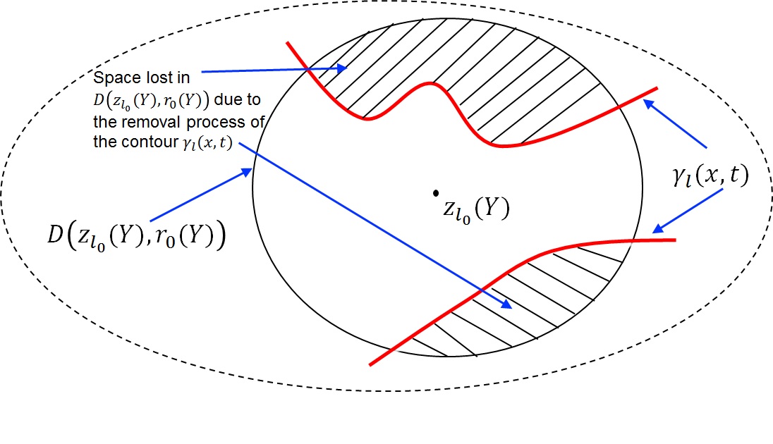
Figure 3.4. Non-availability of the space for $\left\{Y\left(z_{l}(t),\mathbb{C}_{l}\right)\right\}$ in a disc after the time $t_{c}$ due to removal of a piece of contour $\gamma_{l}(x,t)$. The shaded region cannot be reached from $z_{l_{0}}$ within a disc $D\left(z_{l_{0}}(Y),r_{0}(Y)\right)$.

Once $z_{l_{0}}(Y)$ is chosen by $Y\left(z_{l}(t),\mathbb{C}_{l}\right)$, then a disc

(3.51) $$D\left(z_{l_{0}}(Y),r_{0}(Y)\right)\subset\mathbb{C}_{l}$$

will be formed. As the second step $Y\left(z_{l}(t),\mathbb{C}_{l}\right)$ will pick a point within the disc (3.51) such that the points of this disc are all part of the available space in $\mathbb{C}_{l}$ that was available after points (numbers) due to the removal process of the contour $\gamma_{l}(X,t)$ for $t=t_{0}$ to $t=t_{c}$ is implemented. Once $z_{l_{0}}(Y)$ is chosen and the disc (3.51) is formed, there may be situation that the entire space of this disc is not available for choosing $z_{l_{1}}$such that a contour or a piecewise contour can not be formed by joining $z_{l_{0}}$to $z_{l_{1}}.$ The process $\left\{Y\left(z_{l}(t),\mathbb{C}_{l}\right)\right\}$ will have to pick a number randomly only in certain locations of disc. See Figure 3.4. The space within $D\left(z_{l_{0}}(Y),r_{0}(Y)\right)$ is divided into three components, namely, the set of points due to the removal of the space of the contour $\gamma_{l}(X,t)$, say, $S_{1}\left[D\left(z_{l_{0}}(Y),r_{0}(Y)\right)\right]$, the set of points available in the disc to which a contour or piecewise arcs can be drawn from $z_{l_{0}}(Y)$ to $z_{l_{1}}(Y),$ say, $S_{2}\left[D\left(z_{l_{0}}(Y),r_{0}(Y)\right)\right]$, and the set of points available, say, $S_{3}\left[D\left(z_{l_{0}}(Y),r_{0}(Y)\right)\right]$ in the disc to choose $z_{l_{1}}(Y)$ but a contour passing from $z_{l_{0}}(Y)$ to $z_{l_{1}}(Y)$ for $z_{l_{1}}(Y)\in D\left(z_{l_{0}}(Y),r_{0}(Y)\right)$ can not be drawn. The removal process has caused disc $D\left(z_{l_{0}}(Y),r_{0}(Y)\right)$ to write below as a union of these three sets

$$D\left(z_{l_{0}}(Y),r_{0}(Y)\right)=S_{1}\left[D\left(z_{l_{0}}(Y),r_{0}(Y)\right)\right]\cup S_{2}\left[D\left(z_{l_{0}}(Y),r_{0}(Y)\right)\right]\cup$$

(3.52) $$S_{3}\left[D\left(z_{l_{0}}(Y),r_{0}(Y)\right)\right]$$

Here $S_{1},$$S_{2},$ and $S_{3}$ are disjoint. A point (number) to which a contour can be drawn from $z_{l_{0}}(Y)$ is located within the set $S_{2}\left[D\left(z_{l_{0}}(Y),r_{0}(Y)\right)\right].$ Similarly Let be $z_{l_{a}}(Y)$ an arbitrary point available to draw a contour from a previous iteration and was chosen by $\left\{Y\left(z_{l}(t),\mathbb{C}_{l}\right)\right\}$ at some $t$. Using $z_{l_{a}}(Y)$ we can draw a disc $D\left(z_{l_{a}}(Y),r_{a}(Y)\right)$ such that

$$D\left(z_{l_{a}}(Y),r_{a}(Y)\right) =S_{1}\left[D\left(z_{l_{a}}(Y),r_{a}(Y)\right)\right]\cup S_{2}\left[D\left(z_{l_{a}}(Y),r_{a}(Y)\right)\right]\cup$$

$$S_{1}\left[D\left(z_{l_{a}}(Y),r_{a}(Y)\right)\right].$$

If $r_{l}(X,t)\cap D\left(z_{l_{a}}(Y),r_{a}(Y)\right)=\phi\text{ (empty set)},$then

$$S_{1}\left[D\left(z_{l_{a}}(Y),r_{a}(Y)\right)\right]=\phi\text{ and }S_{3}\left[D\left(z_{l_{a}}(Y),r_{a}(Y)\right)\right]=\phi$$

and

$$D\left(z_{l_{a}}(Y),r_{a}(Y)\right)=S_{2}\left[D\left(z_{l_{a}}(Y),r_{a}(Y)\right)\right].$$

Any point in $D\left(z_{l_{a}}(Y),r_{a}(Y)\right)$ can be randomly chosen by $\left\{Y\left(z_{l}(t),\mathbb{C}_{l}\right)\right\}$ such that a contour can be drawn within $D\left(z_{l_{a}}(Y),r_{a}(Y)\right).$ Suppose in a given $D\left(z_{l_{a}}(Y),r_{a}(Y)\right)$, the next iteration point, say, $z_{l_{a^{\prime}}}(Y)$ for $z_{l_{a}}(Y)$ for $z_{l_{a^{\prime}}}(Y)\in D\left(z_{l_{a}}(Y),r_{a}(Y)\right)$ lies such that a direct contour from $z_{l_{a}}(Y)$ to $z_{l_{a^{\prime}}}(Y)$ cannot be drawn due to a deleted space of the contour $\gamma_{l}(X,t).$ Suppose there exists some space outside the deleted space of $\gamma_{l}(X,t)$ within $D\left(z_{l_{a}}(Y),r_{a}(Y)\right)$ so that a piecewise arcs can be drawn from $z_{l_{a}}(Y)$ to $z_{l_{a^{\prime}}}(Y)$. In such situations $Y\left(z_{l}(t),\mathbb{C}_{l}\right)$ will generate a set of points around the deleted space to draw piecewise arcs to join $z_{l_{a}}(Y)$ to $z_{l_{a^{\prime}}}(Y)$ whose distance is

(3.53) $$\int_{a_{0}^{l_{d_{a}}}}^{a_{0}^{l_{d_{a^{\prime}}}}}\left|z[v_{l_{d_{a}}}(Y,\tau)]\right|v^{\prime}_{l_{d_{a^{\prime}}}}(\tau)d\tau.$$

Here (3.53) will be the sum of piecewise arcs such that

$$\int_{a_{0}^{l_{d_{a}}}}^{a_{0}^{l_{d_{a^{\prime}}}}}\left|z[v_{l_{d_{a}}}(Y,\tau)]\right|v^{\prime}_{l_{d_{a^{\prime}}}}(\tau)d\tau =\int_{a_{0}^{l_{d_{a}}}}^{a_{0}^{l_{a(i)}}}\left|z[v_{l_{a(i)}}(Y,\tau)]\right|v^{\prime}_{l_{a(i)}}(\tau)d\tau+$$

$$\sum_{i=1}^{k}\int_{a_{0}^{l_{d_{a(i)}}}}^{a_{0}^{l_{a(i+1)}}}\left|z[v_{l_{a(i+1)}}(Y,\tau)]\right|v^{\prime}_{l_{a(i+1)}}(\tau)d\tau+$$

(3.54) $$\int_{a_{0}^{l_{a(k+1)}}}^{a_{0}^{l_{d_{a^{\prime}}}}}\left|z[v_{l_{d_{a^{\prime}}}}(Y,\tau)]\right|v^{\prime}_{l_{d_{a^{\prime}}}}(\tau)d\tau$$

The process of creation of $\gamma_{l}(Y,t)$ for $t>t_{c}$ continues as described above. Contour $\gamma_{l}(Y,t)$ can have a space of $\gamma_{l}(X,t)$ that does not gets deleted due to the removal process of $X\left(z_{l}(t),\mathbb{C}_{l}\right).$ All the points of the set $\gamma_{l}(X,t)\cap\gamma_{l}(Y,t)$ such that

$$\gamma_{l}(X,t)\cap\gamma_{l}(Y,t)\neq\phi\text{ (empty set)}$$

can get deleted due to the removal process of $X\left(z_{l}(t),\mathbb{C}_{l}\right).$ The process $Y\left(z_{l}(t),\mathbb{C}_{l}\right)$ until a removal process for $Y\left(z_{l}(t),\mathbb{C}_{l}\right)$ is introduced, will not influence the differential equation describing the loss of space in bundle $B_{\mathbb{R}}(\mathbb{C})$ in (LABEL:eq:Db/dtforinfinotelength). Let us introduce removal process for $\gamma_{l}(Y,t)$ at $t=t_{g}$ i.e. starting at the interval $(t_{g-1},t_{g}].$ Suppose a length of this contour equivalent to

$$\int_{a_{0}^{l_{c}}}^{a_{0}^{l_{g}}}\left|z[v_{l_{g}}(Y,\tau)]\right|v^{\prime}_{l_{g}}(\tau)d\tau$$

is always maintained between the new contour formation and removal location of this contour such that removal rate never becomes zero. Suppose $z_{lg(1)}$ be the point chosen in $D\left(z_{l_{g}}(Y),r_{g}(Y)\right)\subset\mathbb{C}_{l}$ where

$$z_{lg(1)}(Y)\in S_{2}\left[D\left(z_{l_{g}}(Y),r_{g}(Y)\right)\right]$$

$$D\left(z_{l_{g}}(Y),r_{g}(Y)\right) =S_{1}\left[D\left(z_{l_{g}}(Y),r_{g}(Y)\right)\right]\cup S_{2}\left[D\left(z_{l_{g}}(Y),r_{g}(Y)\right)\right]\cup$$

(3.55) $$S_{3}\left[D\left(z_{l_{g}}(Y),r_{g}(Y)\right)\right].$$

and

The length from $z_{lg}(Y)$ to $z_{lg(1)}(Y)$ is

(3.56) $$\int_{a_{0}^{l_{g}}}^{a_{0}^{l_{g(1)}}}\left|z[v_{l_{g(1)}}(Y,\tau)]\right|v^{\prime}_{l_{g(1)}}(\tau)d\tau.$$

The removal rate of $Y\left(z_{l}(t),\mathbb{C}_{l}\right)$ we denote here by $\phi(Y,t)$. The value of $\phi(Y,t)$ during $(t_{g},t_{g(1)}]$ is expressed using (3.56) as

$$\phi(Y,t)=\psi(Y,t)\int_{a_{0}^{l_{g}}}^{a_{0}^{l_{g(1)}}}\left|z[v_{l_{g(1)}}(Y,\tau)]\right|v^{\prime}_{l_{g(1)}}(\tau)d\tau,$$

for $0<\psi(Y,t)<1,$ and the value of $\phi(Y,t)$ during $(t_{g},t_{\infty}]$ is expressed using (3.56) as

$$\phi(Y,t)=\psi(Y,t)\int_{a_{0}^{l_{g}}}^{a_{0}^{l_{\infty}}}\left|z[v_{l_{\infty}}(Y,\tau)]\right|v^{\prime}_{l_{\infty}}(\tau)d\tau$$

The dynamics in bundle $B_{\mathbb{R}}(\mathbb{C})$ due to removal of set of points in $\gamma_{l}(X,t)$ $\left(t\in[t_{b},\infty\right)$ and in $\gamma_{l}(Y,t)$ $\left(t\in[t_{g},\infty\right)$described above can be divided into below four parts:

$(i)$ Removal of data points due to the removal process introduced on contour $\gamma_{l}(X,t),$

$(ii)$ Removal of data points due to the removal process introduced on contour $\gamma_{l}(Y,t),$

$(iii)$ Removal of data points in the set $\gamma_{l}(X,t)\cap\gamma_{l}(Y,t)$ for $\gamma_{l}(X,t)\cap\gamma_{l}(Y,t)\neq\phi\text{ (empty set),}$due to the removal process introduced on contour $\gamma_{l}(X,t),$

$(iv)$ Removal of data points in the set $\gamma_{l}(X,t)\cap\gamma_{l}(Y,t)$ for $\gamma_{l}(X,t)\cap\gamma_{l}(Y,t)\neq\phi\text{ (empty set),}$due to the removal process introduced on contour $\gamma_{l}(Y,t).$

Let $\phi(X,t)$ and $\phi(Y,t)$ represent removal rates for the points purely on $\gamma_{l}(x,t)$ and $\gamma_{l}(Y,t)$ and not on $\gamma_{l}(X,t)\cap\gamma_{l}(Y,t)\neq\phi\text{ (empty set).}$Let $\phi_{3}(X,t)$ represent removal rates for the points purely on $\gamma_{l}(X,t)\cap\gamma_{l}(Y,t)\neq\phi\text{ (empty set)}$for the contour initiated by $X\left(z_{l}(t),\mathbb{C}_{l}\right)$ and $\phi_{4}(Y,t)$ represent removal rates for the points purely on $\gamma_{l}(X,t)\cap\gamma_{l}(Y,t)\neq\phi\text{ (empty set)}$ for the contour initiated by $Y\left(z_{l}(t),\mathbb{C}_{l}\right).$ The dynamics in bundle $B_{\mathbb{R}}(\mathbb{C})$ due to four parts above is expressed through the differential equation:

$$\begin{array}[]{cc}\frac{dB_{\mathbb{R}}(\mathbb{C})}{dt}&=B_{\mathbb{R}}(\mathbb{C})-\phi(X,t)B_{\mathbb{R}}(\mathbb{C})-\phi(Y,t)B_{\mathbb{R}}(\mathbb{C})-\phi_{3}(X,t)B_{\mathbb{R}}(\mathbb{C})-\\ &\phi_{4}(Y,t)B_{\mathbb{R}}(\mathbb{C})\\ &=B_{\mathbb{R}}(\mathbb{C})-\left[\psi(X,t)\int_{a_{0}^{l_{0}}}^{a_{0}^{l_{\infty}}}\left|z[v_{l_{\infty}}(X,\tau)]\right|v^{\prime}_{l_{\infty}}(X,\tau)d\tau\right]B_{\mathbb{R}}(\mathbb{C})\\ &-\left[\psi(Y,t)\int_{a_{0}^{l_{g}}}^{a_{0}^{l_{\infty}}}\left|z[v_{l_{\infty}}(Y,\tau)]\right|v^{\prime}_{l_{\infty}}(Y,\tau)d\tau\right]B_{\mathbb{R}}(\mathbb{C})-\psi_{3}(X,t)B_{\mathbb{R}}(\mathbb{C})-\\ &\psi_{4}(Y,t)B_{\mathbb{R}}(\mathbb{C})\\ \\ \end{array}$$

for $0<\psi_{3}(X,t)<1$ and $0<\psi_{4}(Y,t)<1$ in the same time interval in which $\psi(X,t)$ and $\psi(Y,t)$ are implemented.

Theorem 21.

The differential equation

$$\frac{dB_{\mathbb{R}}(\mathbb{C})}{dt}=B_{\mathbb{R}}(\mathbb{C})-\left[\phi(X,t)+\phi(Y,t)+\phi_{3}(X,t)+\phi_{4}(Y,t)\right]B_{\mathbb{R}}(\mathbb{C})$$

where

$$\phi(X,t) =\psi(X,t)\int_{a_{0}^{l_{0}}}^{a_{0}^{l_{\infty}}}\left|z[v_{l_{\infty}}(X,\tau)]\right|v^{\prime}_{l_{\infty}}(X,\tau)d\tau\text{ $\left(0<\psi(X,t)<1\right)$,}$$

$$\phi(Y,t) =\psi(Y,t)\int_{a_{0}^{l_{g}}}^{a_{0}^{l_{\infty}}}\left|z[v_{l_{\infty}}(Y,\tau)]\right|v^{\prime}_{l_{\infty}}(Y,\tau)d\tau\text{ }\left(0<\psi(Y,t)<1\right),$$

$$\phi_{3}(X,t) =0<\psi_{3}(X,t)<1,$$

$$\phi_{4}(Y,t) =0<\psi_{4}(Y,t)<1,$$

will never attain global stability.

Proof.

The removal process continuously removes sets of points of contours $\gamma_{l}(x,t)$ and $\gamma_{l}(y,t)$ described in (LABEL:eq:dB/dtforXY). As in the proof of the Theorem 19, the contour formations happens continuously, and

$$\left|B_{\mathbb{R}}(\mathbb{C})\right|<\epsilon$$

would never arise for every $\epsilon>0$, because of the construction of $\phi(X,t)$, $\phi(Y,t),$ $\phi_{3}(X,t)$, $\phi_{4}(Y,t)$ given in the statement there will be always space of points in $\phi_{4}(Y,t).$ ∎

Remark 22.

One can also develop an argument similar to to the argument in provided in the proof of the Theorem 19 to prove Theorem 21.

Suppose $X^{a}\left(z_{l}(t),\mathbb{C}_{l}\right)$ represents an arbitrary random variable out of infinitely many random variables introduced to form contours with origin in $\mathbb{C}_{l}.$ Let the removal rate of $\gamma_{l}(X^{a},t)$ be $\phi(X^{a},t)$ and $\phi_{3}(X^{a},t)$ be the removal rate of the data points at the intersections of one or more contours. A general differential equation describing the dynamics due to the removal process of points in the bundle is

$$\frac{dB_{\mathbb{R}}(\mathbb{C})}{dt} =B_{\mathbb{R}}(\mathbb{C})-\int_{X^{a}}\phi(X^{a},t)dt[B_{\mathbb{R}}(\mathbb{C})]-$$

(3.58) $$\int_{X^{a}}\phi_{3}(X^{a},t)dt[B_{\mathbb{R}}(\mathbb{C})].$$

In (3.58), the term $\int_{X^{a}}\phi(X^{a},t)dt$ represent the overall removal rates for the infinitely many contours. At the each iteration of the equation (3.58), the quantity $\int_{X^{a}}\phi(X^{a},t)dt$ will be updated based on new removal of a certain contour. Similarly, $\int_{X^{a}}\phi_{3}(X^{a},t)dt$ represent removal rates of the sets of points available at the intersections of the contours.

4. Islands and Holes in $B_{\mathbb{R}}(\mathbb{C})$

The removal process of bundle will create islands of holes due to overlapping (intersections) of infinitely many contours within $B_{\mathbb{R}}(\mathbb{C}).$ These islands will be never be able to reach again by a newly introduced two step randomness. See Figure 4.1.

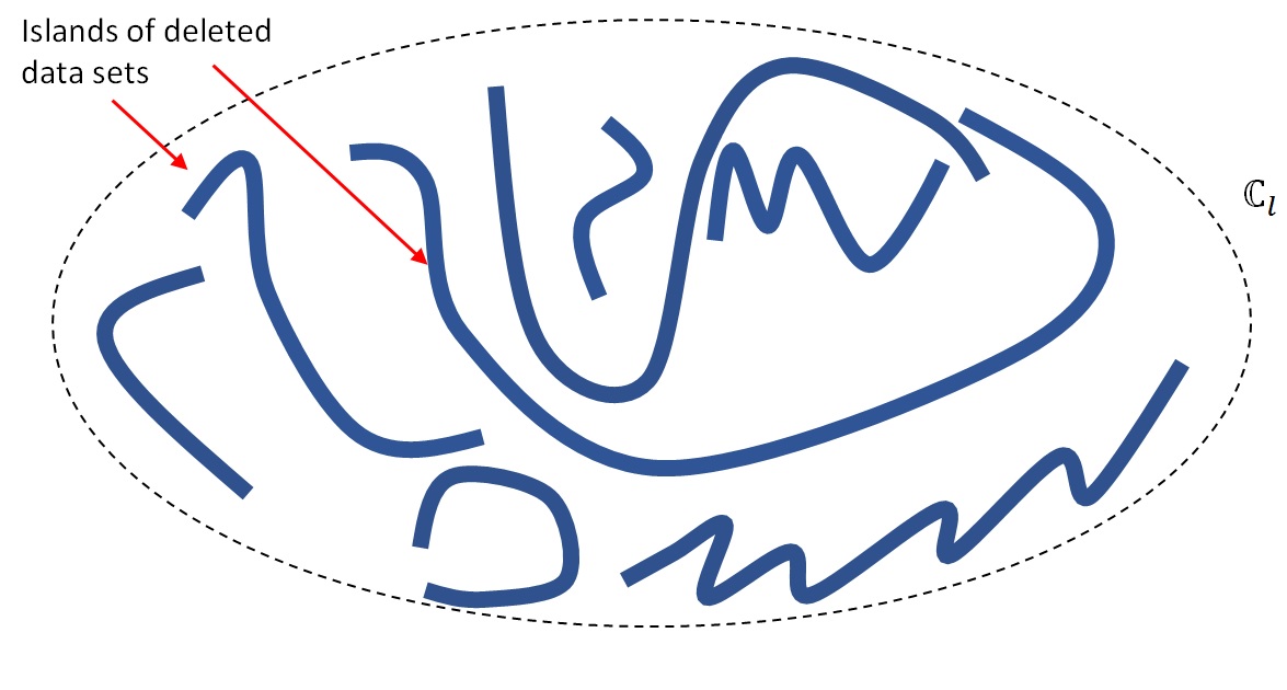
Figure 4.1. Islands of deleted data due to removal process on infinitely many contours.

Suppose we introduce infinitely many random variables of type $X^{a}\left(z_{l}(t),\mathbb{C}_{l}\right)$ that we saw in section 3, but all were introduced at the same time in $\mathbb{C}_{l}.$ Let the number of these random variables be such that they are one to one and onto with each member of the complex plane $\mathbb{C}_{l}.$ Suppose these start creating data for the formation of infinitely many contours. One contour is assumed not to block another contour to use its data points. This is explained further in the following sentences. Suppose $X^{a}\left(z_{l}(t),\mathbb{C}_{l}\right)$ and $X^{b}\left(z_{l}(t),\mathbb{C}_{l}\right)$ be two contours chosen arbitrarily out of these infinitely many contours that were initiated at the same time $t_{0}.$ By construction, they have different origins in $\mathbb{C}_{l}.$ Then the set of complex numbers $\{z_{l}(X^{a},t)\}$ $\left(t\in[t_{0},\infty\right)$ used in the formation of $\gamma_{l}(X^{a},t)$ and the set of numbers used in the formation of $\gamma_{l}(X^{b},t)$ could have a non-empty intersection. That is

$$\left\{z_{l}:z_{l}\in B_{\mathbb{R}}(\mathbb{C}),\text{\{$z_{l}$($X^{a}$,t)\} $\left(t\in(t_{0},\infty\right)$ and }z_{l_{0}}(X^{a})\in\mathbb{C}_{l}\right\}\bigcap$$

$$\left\{z_{l}:z_{l}\in B_{\mathbb{R}}(\mathbb{C}),\text{\{$z_{l}$($X^{b}$,t)\} $\left(t\in(t_{0},\infty\right)$ and }z_{l_{0}}(X^{b})\in\mathbb{C}_{l}\right\}\neq\phi\text{ (empty)}$$

or

$$\left\{z_{l}:z_{l}\in B_{\mathbb{R}}(\mathbb{C}),\text{\{$z_{l}$($X^{a}$,t)\} $\left(t\in(t_{0},\infty)\right)$ and }z_{l_{0}}(X^{a})\in\mathbb{C}_{l}\right\}\bigcap$$

$$\left\{z_{l}:z_{l}\in B_{\mathbb{R}}(\mathbb{C}),\text{\{$z_{l}$($X^{b}$,t)\} $\left(t\in(t_{0},\infty)\right)$ and }z_{l_{0}}(X^{b})\in\mathbb{C}_{l}\right\}\neq\phi\text{ (empty)}$$

Any two contours that have different initial values need not be disjoint. If every $z_{l}(X^{a},t)$ for every $t\in(t_{0},\infty)$ has no overlap with any element of $\{z_{l}(X^{b},t)\}\left(t\in(t_{0},\infty)\right)$ then that could be purely due to the random environment created in section 3. Either of these contours or both could be multilevel contours and have origins in $\mathbb{C}_{l}.$ The formation of multilevel contours and randomness at $\mathbb{C}_{0}\cap\mathbb{C}_{l}$ described earlier remains the same. Two contours might have points of intersection within $B_{\mathbb{R}}(\mathbb{C})$ but such points of intersection need not behave like common points of $\mathbb{C}_{0}\cap\mathbb{C}_{l}\subset B_{\mathbb{R}}(\mathbb{C}).$ This means the set of points on

$$\gamma_{l}(X^{a},t)\cap\gamma_{l}(X^{b},t)$$

for which

$$\gamma_{l}(X^{a},t)\cap\gamma_{l}(X^{b},t)\neq\phi\text{ (empty)}$$

can not be used for changing the plane of the contours. However, the set of points on

(4.3) $$\gamma_{l}(X^{a},t)\cap\gamma_{l}(X^{b},t)\subset\mathbb{C}_{0}$$

for any two arbitrary random variables $X^{a}\left(z_{l}(t),\mathbb{C}_{l}\right)$ and $X^{b}\left(z_{l}(t),\mathbb{C}_{l}\right)$ could behave similarly to the points on $\mathbb{C}_{0}\cap\mathbb{C}_{l}.$ The points on $\mathbb{C}_{0}\cap\mathbb{C}_{p}$ for any arbitrary $\mathbb{C}_{p}\subset B_{\mathbb{R}}(\mathbb{C})$ will have similar properties of forming a multilevel contour as described in section 3.

Suppose

(4.4) $$\gamma_{l}(X^{a},t)\cap\gamma_{l}(X^{b},t)\subset\mathbb{C}_{p}$$

for some arbitrary plane $\mathbb{C}_{p}\subset B_{\mathbb{R}}(\mathbb{C})$ and $\gamma_{l}(X^{a},t)\cap\gamma_{l}(X^{b},t)$ have origins in $\mathbb{C}_{l}.$

Suppose (4.4) satisfied at $t=t_{d},$ then a disc $D\left(z_{l_{d}}(X^{a}),r_{d}(X^{a})\right)$ with center $z_{l_{d}}(X^{a})$ and radius $r_{d}(X^{a})$ is formed such that

(4.5) $$D\left(z_{l_{d}}(X^{a}),r_{d}(X^{a})\right)\subset\mathbb{C}_{p}$$

and next iteration point of $\gamma_{l}(X^{a},t)$ after $z_{l_{d}}(X^{a})$ lies in $\mathbb{C}_{p}$ and not in $\mathbb{C}_{0}\cap\mathbb{C}_{p}$.

Suppose $z_{l_{d^{\prime}}}(X^{a})$ be the point generated after $z_{l_{d^{\prime}}}(X^{a})$ for $z_{l_{d^{\prime}}}(X^{a})\subset D\left(z_{l_{d}}(X^{a}),r_{d}(X^{a})\right)$, then

$$z_{l_{d^{\prime}}}(X^{a})\in\mathbb{C}_{p}\text{ and }z_{l_{d^{\prime}}}(X^{a})\notin\mathbb{C}_{0}\cap\mathbb{C}_{p}.$$

A contour drawn during $[t_{d},t_{d^{\prime}}]$ to reach $z_{l_{d^{\prime}}}(X^{a})$ from $z_{l_{d}}(X^{a})$ with the distance

(4.6) $$\int_{a_{0}^{l_{d}}}^{a_{0}^{l_{d^{\prime}}}}\left|z[u_{l_{d^{\prime}}}(X^{a},\tau)]\right|u^{\prime}_{l_{\infty}}(X^{a},\tau)d\tau\text{ ,}$$

lies on $\mathbb{C}_{p}.$ Here the real valued function $u_{l_{d^{\prime}}}(X^{a},\tau)$ maps $[a_{0}^{l_{d}},a_{0}^{l_{d^{\prime}}})$ onto the interval $[t_{d},t_{d^{\prime}}]$. Because $z_{l_{d}}(X^{a})$ lies on $\gamma_{l}(X^{a},t)$ satisfying (4.4) it could contribute in the next step to form $\gamma_{l}(X^{a},t)$ or $\gamma_{l}(X^{b},t).$ In either situation, the distance in (4.5) lies in $\mathbb{C}_{p}.$ Hence a point in $B_{\mathbb{R}}(\mathbb{C})$ if it is in $\mathbb{C}_{0}\cap\mathbb{C}_{p}$ for some arbitrary $\mathbb{C}_{p}$ have two options to produce a new point on the contour to continue contour formation. The description of the formation of contours at the intersection of $\gamma_{l}(X^{a},t)$ and $\gamma_{l}(X^{b},t)$ is also true if there are more than two intersecting contours. we also note that the lengths of the infinitely many contours up to time $t_{d}$ which were all introduced at $t_{0}$ could have different lengths based on the area of the discs formed, and the point chosen by the corresponding random variable. So the set of lengths

$$\left\{\int_{a_{0}^{l_{d}}}^{a_{0}^{l_{d^{\prime}}}}\left|z[u_{l_{d^{\prime}}}(X^{a},\tau)]\right|u^{\prime}_{l_{d^{\prime}}}(X^{a},\tau)d\tau,\int_{a_{0}^{l_{d}}}^{a_{0}^{l_{d^{\prime}}}}\left|z[u_{l_{d^{\prime}}}(X^{b},\tau)]\right|u^{\prime}_{l_{d^{\prime}}}(X^{b},\tau)d\tau,\cdots\right\}$$

could have different spaces occupied in $B_{\mathbb{R}}(\mathbb{C})$. The location of each contour after some long time $t_{\infty}$ for $t_{\infty}>>t_{d^{\prime}}$ could be anywhere in the bundle and they could be situated in any plane. The set of lengths

$$\left\{\int_{a_{0}^{l_{d}}}^{a_{0}^{l_{\infty}}}\left|z[u_{l_{\infty}}(X^{a},\tau)]\right|u^{\prime}_{l_{\infty}}(X^{a},\tau)d\tau,\int_{a_{0}^{l_{d}}}^{a_{0}^{l_{\infty}}}\left|z[u_{l_{\infty}^{\prime}}(X^{b},\tau)]\right|u^{\prime}_{l_{\infty}}(X^{b},\tau)d\tau,\cdots\right\}$$

and the spaces occupied by

$$\gamma_{l}(X^{a},t),\gamma_{l}(X^{b},t),\cdots,$$

are ever evolving within $B_{\mathbb{R}}(\mathbb{C})$. For a point $z_{l_{d(2)}}(X^{a})$ $\in\mathbb{C}_{p}$ and $z_{l_{d(2)}}(X^{a})$ $\notin\mathbb{C}_{l}\cap\mathbb{C}_{p}$, the equality

$$\int_{a_{0}^{l_{d}}}^{a_{0}^{l_{d(1)}}}\left|z[u_{l_{d(1)}}(X^{a},\tau)]\right|u^{\prime}_{l_{d(1)}}(X^{a},\tau)d\tau +\int_{a_{0}^{l_{d(1)}}}^{a_{0}^{l_{d(2)}}}\left|z[u_{l_{d(2)}}(X^{a},\tau)]\right|u^{\prime}_{l_{d(2)}}(X^{a},\tau)d\tau$$

(4.9) $$=\int_{a_{0}^{l_{d}}}^{a_{0}^{l_{d(2)}}}\left|z[u_{l_{d*(2)}}(X^{a},\tau)]\right|u^{\prime}_{l_{d*(2)}}(X^{a},\tau)d\tau$$

holds for $z_{l_{d}}(X^{a})$ $\in\mathbb{C}_{0}\cap\mathbb{C}_{l}$ and $z_{l_{d(1)}}(X^{a})$ $\in\mathbb{C}_{0}\cap\mathbb{C}_{p}$. For all such $z_{l_{d}}(X^{b})$ $\in\mathbb{C}_{p}$ and $z_{l_{d(2)}}(X^{b})$ $\notin\mathbb{C}_{l}\cap\mathbb{C}_{p}$, and $z_{l_{d}}(X^{b})\neq z_{l_{d}}(X^{a})$, $z_{l_{d(1)}}(X^{b})\neq$ $z_{l_{d(1)}}(X^{a})$, and $z_{l_{d(2)}}(X^{b})$ $\neq z_{l_{d(2)}}(X^{a})$ the equality

$$\int_{a_{0}^{l_{d}}}^{a_{0}^{l_{d(1)}}}\left|z[u_{l_{d(1)}}(X^{b},\tau)]\right|u^{\prime}_{l_{d(1)}}(X^{b},\tau)d\tau +\int_{a_{0}^{l_{d(1)}}}^{a_{0}^{l_{d(2)}}}\left|z[u_{l_{d(2)}}(X^{b},\tau)]\right|u^{\prime}_{l_{d(2)}}(X^{b},\tau)d\tau$$

(4.10) $$=\int_{a_{0}^{l_{d}}}^{a_{0}^{l_{d(2)}}}\left|z[u_{l_{d*(2)}}(X^{b},\tau)]\right|u^{\prime}_{l_{d*(2)}}(X^{b},\tau)d\tau$$

holds for $z_{l_{d}}(X^{b})$ $\in\mathbb{C}_{0}\cap\mathbb{C}_{l}$ and $z_{l_{d(1)}}(X^{b})$ $\in\mathbb{C}_{0}\cap\mathbb{C}_{p}$. From (4.9) and (4.10), we also see that

(4.11) $$\int_{a_{0}^{l_{d}}}^{a_{0}^{l_{d(2)}}}\left|z[u_{l_{d*(2)}}(X^{a},\tau)]\right|u^{\prime}_{l_{d*(2)}}(X^{a},\tau)d\tau$$

$$>\int_{a_{0}^{l_{d(1)}}}^{a_{0}^{l_{d(2)}}}\left|z[u_{l_{d(2)}}(X^{a},\tau)]\right|u^{\prime}_{l_{d(2)}}(X^{a},\tau)d\tau$$

and

(4.12) $$\int_{a_{0}^{l_{d}}}^{a_{0}^{l_{d(2)}}}\left|z[u_{l_{d*(2)}}(X^{b},\tau)]\right|u^{\prime}_{l_{d*(2)}}(X^{b},\tau)d\tau>$$

$$\int_{a_{0}^{l_{d(1)}}}^{a_{0}^{l_{d(2)}}}\left|z[u_{l_{d(2)}}(X^{b},\tau)]\right|u^{\prime}_{l_{d(2)}}(X^{b},\tau)d\tau$$

because the multilevel contours $\gamma_{l}(X^{a},t)$ and $\gamma_{l}(X^{b},t)$ whose distances are in (4.9) and (4.10) has to pass through the plane $\mathbb{C}_{0}\cap\mathbb{C}_{p}.$ For all sets of three numbers of the type for $z_{l_{d}}(X^{b})$, $z_{l_{d(1)}}(X^{b})$, and $z_{l_{d(2)}}(X^{b})$ lying in $\mathbb{C}_{0}\cap\mathbb{C}_{l}$, $\mathbb{C}_{0}\cap\mathbb{C}_{p}$, and $\mathbb{C}_{p},$ for arbitrary $\mathbb{C}_{l}$ and $\mathbb{C}_{p}$ in $B_{\mathbb{R}}(\mathbb{C})$, the equality

(4.13) $$\begin{array}[]{c}\sum_{i=1}^{\infty}\int_{a_{0}^{l_{d}}}^{a_{0}^{l_{d(i)}}}\left|z[u_{l_{d(1)}}(X^{b},\tau)]\right|u^{\prime}_{l_{d(i)}}(X^{b},\tau)d\tau+\\ +\sum_{i=1}^{\infty}\int_{a_{0}^{l_{d(i)}}}^{a_{0}^{l_{d(i+1)}}}\left|z[u_{l_{d(i+1)}}(X^{b},\tau)]\right|u^{\prime}_{l_{d(i+1)}}(X^{b},\tau)d\tau\\ =\sum_{i=1}^{\infty}\int_{a_{0}^{l_{d}}}^{a_{0}^{l_{d(i)}}}\left|z[u_{l_{d*(i)}}(X^{b},\tau)]\right|u^{\prime}_{l_{d*(i)}}(X^{b},\tau)d\tau\end{array}$$

holds, and (4.13) leads to

(4.14) $$\sum_{i=1}^{\infty}\int_{a_{0}^{l_{d}}}^{a_{0}^{l_{d(i)}}}\left|z[u_{l_{d*(i)}}(X^{b},\tau)]\right|u^{\prime}_{l_{d*(i)}}(X^{b},\tau)d\tau>$$

$$\sum_{i=1}^{\infty}\int_{a_{0}^{l_{d(i)}}}^{a_{0}^{l_{d(i+1)}}}\left|z[u_{l_{d(i+1)}}(X^{b},\tau)]\right|u^{\prime}_{l_{d(i+1)}}(X^{b},\tau)d\tau.$$

Consider an arbitrary plane $\mathbb{C}_{q}$ lying somewhere above $\mathbb{C}_{p}$ and $\mathbb{C}_{p}$ lying somewhere above $\mathbb{C}_{l}$ for $\mathbb{C}_{l}$ , $\mathbb{C}_{p}$, and $\mathbb{C}_{q}$ in $B_{\mathbb{R}}(\mathbb{C}),$Let the five points (numbers) in the bundle are arranged as follows:

$$z_{l_{d}}(X^{a})\in\mathbb{C}_{0}\cap\mathbb{C}_{l},z_{l_{d(1)}}(X^{a})\in\mathbb{C}_{0}\cap\mathbb{C}_{p},$$

$$z_{l_{d(2)}}(X^{a}) \notin\mathbb{C}_{0}\cap\mathbb{C}_{p}\text{ and }z_{l_{d(2)}}(X^{a})\in\mathbb{C}_{p},z_{l_{d(3)}}(X^{a})\in\mathbb{C}_{0}\cap\mathbb{C}_{p}\text{ }$$

(reachable from $$z_{l_{d(2)}} X^{a}$$()),

$$z_{l_{d(4)}}(X^{a})\mathbb{C}_{0}\cap\mathbb{C}_{q}\text{, and $z_{l_{d(5)}}$($X^{a}$)$\notin\mathbb{C}_{0}\cap\mathbb{C}_{q}$ and $z_{l_{d(5)}}$($X^{a}$)$\in\mathbb{C}_{p}$.}$$

Then the equality arising out of these points is

$$\int_{a_{0}^{l_{d}}}^{a_{0}^{l_{d(1)}}}\left|z[u_{l_{d(1)}}(X^{a},\tau)]\right|u^{\prime}_{l_{d(1)}}(X^{a},\tau)d\tau+$$

$$\int_{a_{0}^{l_{d(1)}}}^{a_{0}^{l_{d(2)}}}\left|z[u_{l_{d(2)}}(X^{a},\tau)]\right|u^{\prime}_{l_{d(2)}}(X^{a},\tau)d\tau+$$

$$\int_{a_{0}^{l_{d(2)}}}^{a_{0}^{l_{d(3)}}}\left|z[u_{l_{d(3)}}(X^{a},\tau)]\right|u^{\prime}_{l_{d(3)}}(X^{a},\tau)d\tau+$$

$$\int_{a_{0}^{l_{d(3)}}}^{a_{0}^{l_{d(4)}}}\left|z[u_{l_{d(4)}}(X^{a},\tau)]\right|u^{\prime}_{l_{d(4)}}(X^{a},\tau)d\tau+$$

$$\int_{a_{0}^{l_{d(4)}}}^{a_{0}^{l_{d(5)}}}\left|z[u_{l_{d(5)}}(X^{a},\tau)]\right|u^{\prime}_{l_{d(5)}}(X^{a},\tau)d\tau$$

(4.15) $$=\int_{a_{0}^{l_{d}}}^{a_{0}^{l_{d(5)}}}\left|z[u_{l_{d*(5)}}(X^{a},\tau)]\right|u^{\prime}_{l_{d*(5)}}(X^{a},\tau)d\tau$$

where the real valued function $u_{l_{d*}}$maps appropriate time intervals after the parametric representation. For all above such sets of five points in the bundle and for three sets of planes, we will have

$$\sum_{i=1}^{\infty}\int_{a_{0}^{l_{d}}}^{a_{0}^{l_{d(i)}}}\left|z[u_{l_{d(i)}}(X^{a},\tau)]\right|u^{\prime}_{l_{d(i)}}(X^{a},\tau)d\tau+$$

$$\sum_{i=1}^{\infty}\int_{a_{0}^{l_{d(1+i)}}}^{a_{0}^{l_{d(2+i)}}}\left|z[u_{l_{d(2)}}(X^{a},\tau)]\right|u^{\prime}_{l_{d(2)}}(X^{a},\tau)d\tau+$$

$$+\sum_{i=1}^{\infty}\int_{a_{0}^{l_{d(2)}}}^{a_{0}^{l_{d(3)}}}\left|z[u_{l_{d(3)}}(X^{a},\tau)]\right|u^{\prime}_{l_{d(3)}}(X^{a},\tau)d\tau+$$

$$\sum_{i=1}^{\infty}\int_{a_{0}^{l_{d(3+i)}}}^{a_{0}^{l_{d(4+i)}}}\left|z[u_{l_{d(4)}}(X^{a},\tau)]\right|u^{\prime}_{l_{d(4)}}(X^{a},\tau)d\tau+$$

$$\sum_{i=1}^{\infty}\int_{a_{0}^{l_{d(4+i)}}}^{a_{0}^{l_{d(5+i)}}}\left|z[u_{l_{d(5)}}(X^{a},\tau)]\right|u^{\prime}_{l_{d(5)}}(X^{a},\tau)d\tau$$

(4.16) $$=\sum_{i=1}^{\infty}\int_{a_{0}^{l_{d}}}^{a_{0}^{l_{d(5+i)}}}\left|z[u_{l_{d*(5+i)}}(X^{a},\tau)]\right|u^{\prime}_{l_{d*(5+i)}}(X^{a},\tau)d\tau$$

A hole is formed in $B_{\mathbb{R}}(\mathbb{C})$ due to a loss of a set of points (numbers) of data in which a piece of a contour was located (before it got deleted due to a removal process) or a loss of a set of data points of a group a contours. The line consisting of points were lost due to a removal process but all other points around the line or area around a hole could be chosen by a random variable. We introduce and define two new sets, namely, a hole and an island.

Definition 23.

Hole: A hole $H$ is a closed set of points in $B_{\mathbb{R}}(\mathbb{C})$ such that no point of $H$ is available to be chosen by an arbitrary $X^{a}\left(z_{l}(t),\mathbb{C}_{l}\right)$ for an arbitrary plane $\mathbb{C}_{l}.$

Example 24.

Let $\left\{z_{l}(X^{a},t)\right\}$ be the set of numbers of $\gamma_{l}(X^{a},t)$ for $t\in[t_{0},t_{b}$] that got deleted due to a removal process. Then $X^{a}\left(z_{l}(t),\mathbb{C}_{l}\right)$ would not be able to choose a number from $\left\{z_{l}(X^{a},t)\right\}$ for $t\in[t_{0},t_{b}$]. There could be many such holes in $B_{\mathbb{R}}(\mathbb{C}).$ Two or more contours using the same set of points for a period of time, then the removal process of one contour could delete the common set of data so that a hole is formed. We will soon see that the space created by the set $H$ is dynamic.

Definition 25.

Island: Let $S\subset B_{\mathbb{R}}(\mathbb{C})$ and $S\neq\phi\,\text{(empty).}$ The set $S$ is called an island if any element in $S$ is available to be chosen by a random variable but no contour can be drawn from an element within $S$ to an element outside $S,$ say, $S^{c}.$ Here $S,S^{c}\in B_{\mathbb{R}}(\mathbb{C}).$

Example 26.

Consider a disc $D\left(z_{l_{d}}(X^{a}),r_{d}(X^{a})\right)$ with a center $z_{l_{d}}(X^{a})$ chosen by $X^{a}\left(z_{l}(t),\mathbb{C}_{l}\right)$ from a previous iteration. Let two contours $\gamma_{l}(X^{b},t)$ and $\gamma_{l}(X^{c},t)$ pass through $D\left(z_{l_{d}}(X^{a}),r_{d}(X^{a})\right)$ and intersects at two locations (say, $z_{l_{i}}(X^{b})$ and $z_{l_{j}}(X^{b})$ as shown in Figure 4.2. Suppose the spaces of points of $\gamma_{l}(X^{b},t)$ and $\gamma_{l}(X^{c},t)$ passing through $D\left(z_{l_{d}}(X^{a}),r_{d}(X^{a})\right)$ were lost due to respective variables’ removal processes. Then the space formed between these two points of intersections including the data on the contours between $z_{l_{i}}(X^{b})$ and $z_{l_{j}}(X^{b})$ is an island.

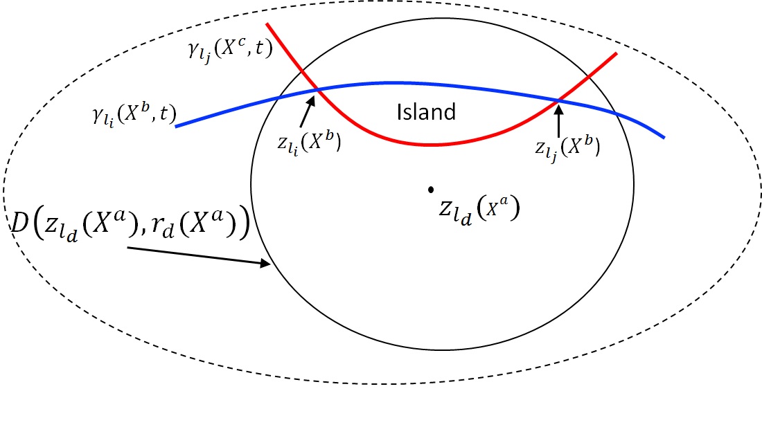
Figure 4.2. An island is created within $D\left(z_{l_{d}}(X^{a}),r_{d}(X^{a})\right).$

The two sets $H$ and $S$ are dynamic as spaces created by these sets could change because of the dynamic nature of contour formation and removal process described in section 3. A time-dependent versions of the definitions for holes and islands can be given here. A set $S(t)$ for $t\in[t_{0},\infty)$ and satisfying the definition 25 can be called an island at $t.$ The set of elements of $S(t_{c})$ for $t_{c}\in[t_{0},\infty)$ satisfying the Definition 25 might lose all its elements in a removal process and might turn into a hole at a time $t_{d}$ for $t_{d}>t_{c}.$ If $S(t)$is an island then no one cannot draw a contour from the elements of $S(t)$ to an element in $S^{c}(t)$ where

(4.17) $$S^{c}(t)=\left\{z:z\notin S(t)\subset B_{\mathbb{R}}(\mathbb{C})\text{ and }z\in B_{\mathbb{R}}(\mathbb{C})\right\}.$$

Similarly, a contour cannot be drawn from an element (point) of $S^{c}(t)$ to an element in $S(t).$ The spaces of $S(t)$ and $S^{c}(t)$ are separated by $H.$ The area of a hole could change over a time as more data points removed are added to a specific hole.

Theorem 27.

Suppose a disc $D\left(z_{l_{d}}(X^{a}),r_{d}(X^{a})\right)$ formed out of $X^{a}\left(z_{l}(t),\mathbb{C}_{l}\right)$ is given. Let $z_{l_{1}}$ and $z_{l_{2}}$ be two points in the boundary set of $D.$ A contour $C_{1}$ formed by an arbitrary process $X^{b}\left(z_{l}(t),\mathbb{C}_{l}\right)$ enters the disc through $z_{l_{1}}$ and leaves the disc from $z_{l_{2}}$ and another contour $C_{2}$ formed by an arbitrary process $X^{c}\left(z_{l}(t),\mathbb{C}_{l}\right)$ enters the disc through $z_{l_{1}}$ and leaves the disc from $z_{l_{2}}.$ The paths of $C_{1}$ and $C_{2}$ never meet except at the points $z_{l_{1}}$ and $z_{l_{2}}$ and the center $z_{l_{d}}(X^{a})$ lies in between the contours. Suppose the removal process of two contours $C_{1}$ and $C_{2}$ introduced such that $C_{1}\cup C_{2}$ form a hole at $t$. Then, the set of points lying between $C_{1}$ and $C_{2}$ forms an island.

Proof.

Given that $z_{l_{1}}$ and $z_{l_{2}}$are located on the boundary of the disc $D\left(z_{l_{d}}(X^{a}),r_{d}(X^{a})\right)$ and $z_{l_{d}}(X^{a})$ is located in between $C_{1}$ and $C_{2}.$ See Figure 4.3 for a description of given information and locations of $z_{l_{1}}$ and $z_{l_{2}}.$

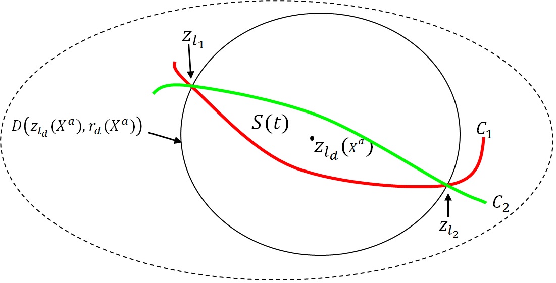
Figure 4.3. Formation of an island due to a removal process of Theorem 27.

Let $S(t)$ be a set in $D\left(z_{l_{d}}(X^{a}),r_{d}(X^{a})\right)$ that consists of all points in between $C_{1}$ and $C_{2}$ as shown in Figure 4.3. The set $D\left(z_{l_{d}}(X^{a}),r_{d}(X^{a})\right)\backslash S(t)$ will consists of points as in (LABEL:eq:4-19),

$$D\left(z_{l_{d}}(X^{a}),r_{d}(X^{a})\right)\backslash S(t)=\left\{z_{l}:z_{l}\in D\left(z_{l_{d}}(X^{a}),r_{d}(X^{a})\right)\text{ and }z_{l}\notin S(t)\right\}.$$

The disc $D\left(z_{l_{d}}(X^{a}),r_{d}(X^{a})\right)$ can be partitioned into disjoint union of three sets as below

$$D\left(z_{l_{d}}(X^{a}),r_{d}(X^{a})\right)=\left[D\left(z_{l_{d}}(X^{a}),r_{d}(X^{a})\right)\backslash S(t)\right]\cup S(t)\cup\left[C_{1}\cup C_{2}\right].$$

By the construction, we cannot draw a contour from a point in $S(t)$ to a point in

$$D\left(z_{l_{d}}(X^{a}),r_{d}(X^{a})\right)\backslash S(t).$$

Hence, $S(t)$ is an island. ∎

Theorem 28.

The union of collection of all holes within $B_{\mathbb{R}}(\mathbb{C})$ is compact.

Proof.

Each hole is a closed set of points from a contour or a collection of contours. Let $H_{\alpha}$ be an arbitrary hole. An infinite union of such holes,

(4.20) $$\bigcup_{\alpha}H_{\alpha}.$$

is closed. Each $H_{\alpha}$ at time $t$ is bounded by the length of the contour formed until the time $t+1$, because the removal process follows contour formation with some lag in the time. So

(4.21) $$\left|\bigcup_{\alpha}H_{\alpha}\right|<\int_{a_{0}^{l_{d}}}^{a_{0}^{l_{d(t+i)}}}\left|z[u_{l_{d(t+i)}}(X^{a},\tau)]\right|u^{\prime}_{l_{d(5+i)}}(X^{a},\tau)d\tau,$$

for an arbitrary process $X^{a}\left(z_{l}(t),\mathbb{C}_{l}\right)$. So the union of a collection of holes is bounded. Hence, such a collection is compact. ∎

Theorem 29.

Suppose infinitely many random variables of the type $X^{a}\left(z_{l}(t),\mathbb{C}_{l}\right)$ are introduced one by one as in Section 3. If every point within an island $S(t)$ is part of a contour at time $t$, then due to a removal process $S(t)$ becomes $H(t_{c})$ for $t_{c}>t.$

Proof.

Given there is a $S(t)$ at time $t.$ Let there be finitely many contours passing through the region $S(t)$ such that all the points of $S(t)$ are in one or more of the contours. Once a removal process is introduced at $t_{c}>t$ then all the points of $S(t)$ will not be available for a new random variable. Hence, $S(t)$ will asymptotically become a hole. ∎

Let us introduce a removal process for the infinitely many contours introduced earlier in this section. These contours were all started at the same time $t_{0}$. The number of such contours is equivalent to the set of elements in $\mathbb{C}_{l}.$ Some of the elements in $\mathbb{C}_{l}$ are also in $\mathbb{C}_{0}\cap\mathbb{C}_{l}.$ Note that,

(4.22) $$\mathbb{C}_{l}=\left(\mathbb{C}_{0}\cap\mathbb{C}_{l}\right)\cup\mathbb{C}_{l}=\left\{z_{l}:z_{l}\in\mathbb{C}_{l}\text{ or }z_{l}\in\mathbb{C}_{0}\cap\mathbb{C}_{l}\right\}.$$

So removing a contour data that was formed from $t_{0}$ until a time $t_{c}$ at a rate $\phi(X^{a},t)$ for an arbitrary random variable $X^{a}\left(z_{l}(t),\mathbb{C}_{l}\right)$ would also remove contour data that is located in the set $\mathbb{C}_{0}\cap\mathbb{C}_{l}.$ We described earlier how the islands of sets of data could be formed, and formation of islands could happen in distinct time intervals once removal process is introduced.

Remember that all the contours have origin in $\mathbb{C}_{l}$ only. Now at $t_{c}$ due to a removal process, the points of $\mathbb{C}_{l}$ are not available to be chosen by any of the infinitely many random variables. The paths of these random variables are not disjoint. Some of these random variables may be in another plane outside $\mathbb{C}_{l}$at $t=t_{c}.$ Contour formations of these infinitely many random variables of type $X^{a}\left(z_{l}(t),\mathbb{C}_{l}\right)$ may continue even after $t_{c}$ because of their presence in outside $\mathbb{C}_{l}$ at $t=t_{c}.$ So the entire plane $\mathbb{C}_{l}$ is not available in the bundle $B_{\mathbb{R}}(\mathbb{C})$. So the remaining space formed will be the set of points $B_{\mathbb{R}}(\mathbb{C})\backslash\mathbb{C}_{l},$ where

(4.23) $$B_{\mathbb{R}}(\mathbb{C})\backslash\mathbb{C}_{l}=\left\{z_{l}:z_{l}\in B_{\mathbb{R}}(\mathbb{C})\text{ and }z_{l}\in\mathbb{C}_{l}\right\}$$

4.1. Consequences of $B_{\mathbb{R}}(\mathbb{C})\backslash\mathbb{C}_{l}$ on Multilevel Contours

At the time of $t=t_{c},$ there could be one of the following two situations for the status of infinitely many random variables that were introduced at $t_{0}.$

$(i)$ All the contours formed until $t_{c}$ are active only in $\mathbb{C}_{l}$ at $t=t_{c}$ and for any arbitrary $X^{a}\left(z_{l}(t),\mathbb{C}_{l}\right)$ the set of points $\left\{z_{l}\left(X^{a},t\right)\right\}$ for $t\in[t_{0},t_{c}]$ are in $\mathbb{C}_{l},$ i.e.

(4.24) $$\left\{z_{l}\left(X^{a},t\right)\right\}\text{}\left(t\in[t_{0},t_{c}]\right)\subset\mathbb{C}_{l}.$$

This means, no contour has crossed the plane until $t=t_{c}.$

$(ii)$ Only a fraction of infinitely many random variables are active in $\mathbb{C}_{l}$ at $t=t_{c},$ and the rest of all random variables are active outside $\mathbb{C}_{l}.$

If every contour satisfies the above situation $(i)$ at $t=t_{c},$ then due to the removal process all the points in $\mathbb{C}_{l}$cannot be reached to form a contour. In such a situation, the plane $\mathbb{C}_{l}$ forms a hole, and the contours formation process halts. Suppose only a fraction of infinitely many random variables, say, $\alpha_{1}$ are inside $\mathbb{C}_{l}$ at $t_{c}$, then there will be two options for the location of those random variables (i.e. for the fraction $(1-\alpha_{1}$) which are outside $\mathbb{C}_{l}$ at $t_{c}.$ A fraction of them, say, $\alpha_{2}$ will be above $\mathbb{C}_{l}$ and the remaining fraction $(1-\alpha_{2})$ of the random variables will be somewhere in a plane below $\mathbb{C}_{l}.$ Let $T$ be the set of all contours active $t_{c}$ and $\alpha_{1}$ be the fraction of them active and located in $\mathbb{C}_{l},$ then $(1-\alpha_{1})\left|T\right|$ be the set of contours that are active and outside $\mathbb{C}_{l}.$ Then, $(1-\alpha_{1})\left|T\right|$ are further divided as

(4.25) $$(1-\alpha_{1})\left|T\right|=\alpha_{2}\left[(1-\alpha_{1})\left|T\right|\right]+(1-\alpha_{2})\left[(1-\alpha_{1})\left|T\right|\right],$$

where $\alpha_{2}$ is the fraction of contours that are active at $t_{c}$ and are located somewhere in a plane above $\mathbb{C}_{l},$ and $1-\alpha_{2}$ is the fraction of contours that are active at $t_{c}$ and are located somewhere in a plane below $\mathbb{C}_{l}.$ Because the plane $\mathbb{C}_{l}$ became a hole, the set of contours, say, $T_{\alpha_{1}}$denoted to represent $\alpha_{1}\left|T\right|$ number of contours will stop further formation for $t>t_{c}.$ The set of contours, say, $T_{1-\alpha_{1}}$ will be active outside $\mathbb{C}_{l}$, where

(4.26) $$T_{1-\alpha_{1}}=T_{\alpha_{2}}\cup T_{1-\alpha_{2}}.$$

Here $T_{\alpha_{2}}$ represent the set of contours that are located somewhere in a plane above $\mathbb{C}_{l},$ $T_{1-\alpha_{2}}$ represent the set of contours that are located somewhere in a plane below $\mathbb{C}_{l}.$ The carnality of $T_{1-\alpha_{1}}$is constant for $t>t_{c},$ so as the cardinals of $T_{\alpha_{2}}$ and $T_{1-\alpha_{2}}$ at $t>t_{c}.$We also partition the set of elements in $B_{\mathbb{R}}(\mathbb{C})$ at $t>t_{c}$ as

(4.27) $$\left.B_{\mathbb{R}}(\mathbb{C})\right|_{t>t_{c}}=B_{\mathbb{R}}(\mathbb{C},\alpha_{2})\cup B_{\mathbb{R}}(\mathbb{C},1-\alpha_{2}),$$

where as

(4.28) $$B_{\mathbb{R}}(\mathbb{C})=B_{\mathbb{R}}(\mathbb{C},\alpha_{2})\cup\mathbb{C}_{l}\cup B_{\mathbb{R}}(\mathbb{C},1-\alpha_{2}),$$

where $B_{\mathbb{R}}(\mathbb{C},\alpha_{2})\subset B_{\mathbb{R}}(\mathbb{C})$ is the set of planes which are above $\mathbb{C}_{l},$ and $B_{\mathbb{R}}(\mathbb{C},1-\alpha_{2})\subset B_{\mathbb{R}}(\mathbb{C})$ is the set of planes which are above $\mathbb{C}_{l}.$ The set of contours that are active after $t_{c}$ are located in the set, say $B_{\mathbb{R}}(\mathbb{C},1-\alpha_{1})$ and from (4.27), we have

(4.29) $$B_{\mathbb{R}}(\mathbb{C},1-\alpha_{2})=\left.B_{\mathbb{R}}(\mathbb{C})\right|_{t>t_{c}}.$$

As described above, contour formations and removal processes of the contours in $B_{\mathbb{R}}(\mathbb{C},1-\alpha_{2})$ will continue. Due to presence of the hole $\mathbb{C}_{l},$ the active contours of $B_{\mathbb{R}}(\mathbb{C},\alpha_{2})$ and $B_{\mathbb{R}}(\mathbb{C},1-\alpha_{2})$ will not have any further intersecting points. The tails of the contours remaining in $B_{\mathbb{R}}(\mathbb{C},\alpha_{2})$ and $B_{\mathbb{R}}(\mathbb{C},1-\alpha_{2})$ will be eventually lost for some time after $t_{c}.$ Let $\gamma_{l}(X^{a},t)$ be an arbitrary contour that is active in $B_{\mathbb{R}}(\mathbb{C},\alpha_{2})$, and was created by $X^{a}.$ Suppose the set of points touched by the contour $\gamma_{l}(X^{a},t)$ prior to $t_{c}$ were located in $B_{\mathbb{R}}(\mathbb{C},\alpha_{2})$, $\mathbb{C}_{l}$, and $B_{\mathbb{R}}(\mathbb{C},1-\alpha_{2}),$ this contour is described by $z_{l}(X^{a},t)$ $\left(t\in[t_{0},\infty)\right)$ and $t=u_{l_{c}}(X^{a},\tau)$ $\left(a_{0}\leq\tau\leq a_{c}\right)$ is the parametric representation for $\gamma_{l}(X^{a},t)$ with a real values function $u_{l}(X^{a},\tau)$ mapping $[a_{0},a_{c}]$ onto the interval $[t_{0},t_{c}].$ Let $L\left(\gamma_{l}(X^{a},t)\left(t\in[t_{0},t_{c}]\right)\right)$ represent the length of $\gamma_{l}(X^{a},t)\left(t\in[t_{0},t_{c}]\right)$ up to $t_{c},$ then

(4.30) $$L\left(\gamma_{l}(X^{a},t)\left(t\in[t_{0},t_{c}]\right)\right)=\int_{a_{0}}^{a_{c}}\left|z[u_{l_{c}}(X^{a},\tau)]\right|u^{\prime}_{l_{c}}(X^{a},\tau)d\tau$$

had covered points from each disjoint set of $B_{\mathbb{R}}(\mathbb{C})$ in (4.28). Let us assume that $\gamma_{l}(X^{a},t)\left(t\in[t_{0},t_{c}]\right)$ has visited a multiple number of times through each of the sets of (4.28) before in remained active in $B_{\mathbb{R}}(\mathbb{C},\alpha_{2})$ at $t=t_{c}.$ Then $L\left(\gamma_{l}(X^{a},t)\left(t\in[t_{0},t_{c}]\right)\right)$ in (4.30) can be expressed as three components where each component is made up of several contour integrals. Since $\gamma_{l}(X^{a},t)$ had visited each portion in (4.30) several times, the length $L\left(\gamma_{l}(X^{a},t)\left(t\in[t_{0},t_{c}]\right)\right)$ in (4.30) is distributed into corresponding parts.The first part consists of the sum of all the lengths of piecewise contours of (4.30) lying in $\mathbb{C}_{l}$, say, $L\left(\gamma_{l}(X^{a},t,\alpha_{1})\left(t\in[t_{0},t_{c}]\right)\right)$, and can be computed using

$$L\left(\gamma_{l}(X^{a},t,\alpha_{1})\left(t\in[t_{0},t_{c}]\right)\right) =\int_{a(0)}^{a(1)}\left|z[u_{l_{a(1)}}(X^{a},\tau)]\right|u^{\prime}_{l_{a(1)}}(X^{a},\tau)d\tau+$$

(4.31) $$\sum_{i\in A(\alpha_{1})}\int_{a(i)}^{a(i+1)}\left|z[u_{l_{a(i+1)}}(X^{a},\tau)]\right|u^{\prime}_{l_{a(i+1)}}(X^{a},\tau)d\tau,$$

where $u_{l_{a(1)}}(X^{a},\tau)$ and $u_{l_{a(i+1)}}(X^{a},\tau)$ are the real valued functions used in parametric representations with corresponding onto mappings. The notation $i\in A(\alpha_{1})$ indicates summing the length over all the piecewise contours in the set $A(\alpha_{1}).$ The set $A(\alpha_{1})$ consists of all the piecewise contours of $X^{a}\left(z_{l}(t),\mathbb{C}_{l}\right)$ until $t_{c}$ that are lying in $\mathbb{C}_{l}.$ The first integral on the R.H.S of (4.31) is the length of the piecewise contour from its origin to the entry point either in $B_{\mathbb{R}}(\mathbb{C},\alpha_{2})$ or in $B_{\mathbb{R}}(\mathbb{C},1-\alpha_{2})$. The sum of integrals on the R.H.S of (4.31) is the total length of the piecewise contours due to $A(\alpha_{1}).$ The second part in (4.30) consists of piecewise contours in $B_{\mathbb{R}}(\mathbb{C},\alpha_{2})$ whose total length, say, $L\left(\gamma_{l}(X^{a},t,\alpha_{2})\left(t\in[t_{0},t_{c}]\right)\right)$, is computed as

$$L\left(\gamma_{l}(X^{a},t,\alpha_{2})\left(t\in[t_{0},t_{c}]\right)\right) =\sum_{i\in A(\alpha_{2})}\int_{a(i)}^{a(i+1)}\left|z[u_{l_{a(i+1)}}(X^{a},\tau)]\right|u^{\prime}_{l_{a(i+1)}}(X^{a},\tau)d\tau+$$

(4.32) $$\int_{a_{c-1}}^{a_{c}}\left|z[u_{l_{c}}(X^{a},\tau)]\right|u^{\prime}_{l_{c}}(X^{a},\tau)d\tau$$

The set $A(\alpha_{2})$ in (4.32) consists of all the piecewise contours of $X^{a}\left(z_{l}(t),\mathbb{C}_{l}\right)$ until $t_{c}$ that are lying in $B_{\mathbb{R}}(\mathbb{C},\alpha_{2}).$ The second integral in the R.H.S. of (4.32) consists of length of the last piece of the contour $\gamma_{l}(X^{a},t)$ until $t=t_{c}$ in $B_{\mathbb{R}}(\mathbb{C},\alpha_{2}).$ Here $u_{l_{c}}(X^{a},\tau)$ is the real valued function used in parametric representations with corresponding onto mappings. The third part in (4.30) consists of piecewise contours in $B_{\mathbb{R}}(\mathbb{C},1-\alpha_{2})$ whose total length, say, $L\left(\gamma_{l}(X^{a},t,1-\alpha_{2})\left(t\in[t_{0},t_{c}]\right)\right)$, is computed as

(4.33) $$\begin{array}[]{c}L\left(\gamma_{l}(X^{a},t,1-\alpha_{2})\left(t\in[t_{0},t_{c}]\right)\right)\\ \sum_{i\in A(1-\alpha_{2})}\int_{a(i)}^{a(i+1)}\left|z[u_{l_{a(i+1)}}(X^{a},\tau)]\right|u^{\prime}_{l_{a(i+1)}}(X^{a},\tau)d\tau.\end{array}$$

Hence the length in (4.30) can be expressed using (4.31), (4.32), and (4.33) as

$$L\left(\gamma_{l}(X^{a},t)\left(t\in[t_{0},t_{c}]\right)\right) =\int_{a(0)}^{a(1)}\left|z[u_{l_{a(1)}}(X^{a},\tau)]\right|u^{\prime}_{l_{a(1)}}(X^{a},\tau)d\tau+$$

$$\sum_{i\in A(\alpha_{1})}\int_{a(i)}^{a(i+1)}\left|z[u_{l_{a(i+1)}}(X^{a},\tau)]\right|u^{\prime}_{l_{a(i+1)}}(X^{a},\tau)d\tau+$$

$$=\sum_{i\in A(\alpha_{2})}\int_{a(i)}^{a(i+1)}\left|z[u_{l_{a(i+1)}}(X^{a},\tau)]\right|u^{\prime}_{l_{a(i+1)}}(X^{a},\tau)d\tau+$$

$$\int_{a_{c-1}}^{a_{c}}\left|z[u_{l_{c}}(X^{a},\tau)]\right|u^{\prime}_{l_{c}}(X^{a},\tau)d\tau+$$

(4.34) $$\sum_{i\in A(1-\alpha_{2})}\int_{a(i)}^{a(i+1)}\left|z[u_{l_{a(i+1)}}(X^{a},\tau)]\right|u^{\prime}_{l_{a(i+1)}}(X^{a},\tau)d\tau.$$

Due to the hole $\mathbb{C}_{l}$ created in the bundle $B_{\mathbb{R}}(\mathbb{C})$, the remaining length of the contour that will be subjected to removal process is obtained by removing the sum of piecewise contour lengths in $\mathbb{C}_{l},$ and is given by

$$L\left(\gamma_{l}(X^{a},t)\left(t\in[t_{0},t_{c}]\right)\right) =\sum_{i\in A(\alpha_{2})}\int_{a(i)}^{a(i+1)}\left|z[u_{l_{a(i+1)}}(X^{a},\tau)]\right|u^{\prime}_{l_{a(i+1)}}(X^{a},\tau)d\tau+$$

$$\int_{a_{c-1}}^{a_{c}}\left|z[u_{l_{c}}(X^{a},\tau)]\right|u^{\prime}_{l_{c}}(X^{a},\tau)d\tau+$$

(4.35) $$\sum_{i\in A(1-\alpha_{2})}\int_{a(i)}^{a(i+1)}\left|z[u_{l_{a(i+1)}}(X^{a},\tau)]\right|u^{\prime}_{l_{a(i+1)}}(X^{a},\tau)d\tau.$$

Since $\gamma_{l}(X^{a},t)$ is active in $B_{\mathbb{R}}(\mathbb{C},\alpha_{2})$, the formation of the contour will continue forever and the sum of the pieces of the lengths of $\gamma_{l}(X^{a},t)$ that is there in $B_{\mathbb{R}}(\mathbb{C},1-\alpha_{2})$ will be deleted from $B_{\mathbb{R}}(\mathbb{C},1-\alpha_{2}).$ This deletion could be according to a removal function $\phi(X^{a},t,1-\alpha_{2})$ similar to the procedure explained in (3.48). The differential equation to model the space of points lost due to a removal process $\phi(X^{a},t,1-\alpha_{2})$ is

$$\left.\frac{dB_{\mathbb{R}}(\mathbb{C},1-\alpha_{2})}{dt}\right|_{\phi(X^{a},t,1-\alpha_{2})}=\left.B_{\mathbb{R}}(\mathbb{C},1-\alpha_{2})\right|_{t=t_{c}}-\phi(X^{a},t)\left.B_{\mathbb{R}}(\mathbb{C},1-\alpha_{2})\right|_{t=t_{c}}$$

for

$$\phi(X^{a},t,1-\alpha_{2})=\psi(X^{a},t,1-\alpha_{2})\times$$

$$\sum_{i\in A(1-\alpha_{2})}\int_{a(i)}^{a(i+1)}\left|z[u_{l_{a(i+1)}}(X^{a},\tau)]\right|u^{\prime}_{l_{a(i+1)}}(X^{a},\tau)d\tau\text{ $\left(t\in(t_{c},t_{c^{\prime}}]\right)$}.$$

for $0<\psi(X^{a},t,1-\alpha_{2})<1.$ Suppose $\gamma_{l}(X^{a},t)$ is active in $B_{\mathbb{R}}(\mathbb{C},1-\alpha_{2})$ instead of in $B_{\mathbb{R}}(\mathbb{C},\alpha_{2}).$ As in above, the set of points touched by the contour $\gamma_{l}(X^{a},t)$ prior to $t_{c}$ would have located in $B_{\mathbb{R}}(\mathbb{C},\alpha_{2})$, $\mathbb{C}_{l}$, and $B_{\mathbb{R}}(\mathbb{C},1-\alpha_{2}).$ We described this contour by $z_{l}(X^{a},t)$ $\left(t\in[t_{0},\infty)\right)$ and $t=w_{l_{c}}(X^{a},\tau)$ $\left(a^{\prime}_{0}\leq\tau\leq a^{\prime}_{c}\right)$ is the parametric representation for $\gamma_{l}(X^{a},t)$ with a real values function $w_{l_{c}}(X^{a},\tau)$ mapping $[a^{\prime}_{0},a^{\prime}_{c}]$ onto the interval $[t_{0},t_{c}].$ Let $L\left(\gamma_{l}(X^{a},t,1-\alpha_{2})\left(t\in[t_{0},t_{c}]\right)\right)$ represent the length of $\gamma_{l}(X^{a},t)\left(t\in[t_{0},t_{c}]\right)$ up to $t_{c},$ then

$$L\left(\gamma_{l}(X^{a},t,1-\alpha_{2})\left(t\in[t_{0},t_{c}]\right)\right)=\int_{a^{\prime}_{0}}^{a^{\prime}_{c}}\left|z[w_{l_{c}}(X^{a},\tau)]\right|w^{\prime}_{l_{c}}(X^{a},\tau)d\tau$$

had covered points from each disjoint set of $B_{\mathbb{R}}(\mathbb{C})$ in (4.28). As in above, let us assume that $\gamma_{l}(X^{a},t)\left(t\in[t_{0},t_{c}]\right)$ has visited a multiple number of times through each of the sets of (4.28) before in remained active in $B_{\mathbb{R}}(\mathbb{C},1-\alpha_{2})$ at $t=t_{c}.$ Then $L\left(\gamma_{l}(X^{a},t,1-\alpha_{2})\left(t\in[t_{0},t_{c}]\right)\right)$ in (LABEL:eq:4-39) can be expressed as three components where each component is made up of several contour integrals. Since $\gamma_{l}(X^{a},t)$ had visited each portion in (LABEL:eq:4-39) several times, the length $L\left(\gamma_{l}(X^{a},t,1-\alpha_{2})\left(t\in[t_{0},t_{c}]\right)\right)$ in (LABEL:eq:4-39) is distributed into corresponding parts.The first part consists of the sum of all the lengths of piecewise contours of (LABEL:eq:4-39) lying in $\mathbb{C}_{l}$, say, $L\left(\gamma_{l}(X^{a},t,\alpha_{1})\left(t\in[t_{0},t_{c}]\right)\right)$, and can be computed using

$$L\left(\gamma_{l}(X^{a},t,\alpha_{1})\left(t\in[t_{0},t_{c}]\right)\right) =\int_{a^{\prime}(0)}^{a^{\prime}(1)}\left|z[w_{l_{a^{\prime}(1)}}(X^{a},\tau)]\right|w^{\prime}_{l_{a^{\prime}(1)}}(X^{a},\tau)d\tau+$$

(4.39) $$\sum_{i\in A^{\prime}(\alpha_{1})}\int_{a^{\prime}(i)}^{a^{\prime}(i+1)}\left|z[w_{l_{a(i+1)}}(X^{a},\tau)]\right|w^{\prime}_{l_{a(i+1)}}(X^{a},\tau)d\tau,$$

where $w_{l_{a^{\prime}(1)}}(X^{a},\tau)$ and $w_{l_{a^{\prime}(i+1)}}(X^{a},\tau)$ are the real valued functions used in parametric representations with corresponding onto mappings. The notation $i\in A^{\prime}(\alpha_{1})$ indicates summing the length over all the piecewise contours in the set $A^{\prime}(\alpha_{1}).$ The set $A^{\prime}(\alpha_{1})$ consists of all the piecewise contours of $X^{a}\left(z_{l}(t),\mathbb{C}_{l}\right)$ until $t_{c}$ that are lying in $\mathbb{C}_{l}.$ The first integral on the R.H.S of (4.39) is the length of the piecewise contour from its origin to the entry point either in $B_{\mathbb{R}}(\mathbb{C},\alpha_{2})$ or in $B_{\mathbb{R}}(\mathbb{C},1-\alpha_{2})$. The sum of integrals on the R.H.S of (4.39) is the total length of the piecewise contours due to $A^{\prime}(\alpha_{1}).$ The second part in (LABEL:eq:4-39) consists of piecewise contours in $B_{\mathbb{R}}(\mathbb{C},1-\alpha_{2})$ whose total length, say, $L\left(\gamma_{l}(X^{a},t,1-\alpha_{2})\left(t\in[t_{0},t_{c}]\right)\right)$, is computed as

(4.40) $$\begin{array}[]{c}L\left(\gamma_{l}(X^{a},t,1-\alpha_{2})\left(t\in[t_{0},t_{c}]\right)\right)=\\ \sum_{i\in A^{\prime}(1-\alpha_{2})}\int_{a^{\prime}(i)}^{a^{\prime}(i+1)}\left|z[w_{l_{a^{\prime}(i+1)}}(X^{a},\tau)]\right|w^{\prime}_{l_{a^{\prime}(i+1)}}(X^{a},\tau)d\tau+\\ \int_{a^{\prime}_{c-1}}^{a^{\prime}_{c}}\left|z[w_{l_{c}}(X^{a},\tau)]\right|w^{\prime}_{l_{c}}(X^{a},\tau)d\tau\end{array}$$

Note that the contour is active in $B_{\mathbb{R}}(\mathbb{C},1-\alpha_{2})$. The set $A^{\prime}(\alpha_{2})$ in (4.40) consists of all the piecewise contours of $X^{a}\left(z_{l}(t),\mathbb{C}_{l}\right)$ until $t_{c}$ that are lying in $B_{\mathbb{R}}(\mathbb{C},1-\alpha_{2}).$ The second integral in the R.H.S. of (4.40) consists of length of the last piece of the contour $\gamma_{l}(X^{a},t)$ until $t=t_{c}$ in $B_{\mathbb{R}}(\mathbb{C},1-\alpha_{2}).$ Here $w_{l_{c}}(X^{a},\tau)$ is the real valued function used in parametric representations with corresponding onto mappings. The third part in (LABEL:eq:4-39) consists of piecewise contours in $B_{\mathbb{R}}(\mathbb{C},\alpha_{2})$ whose total length, say, $L\left(\gamma_{l}(X^{a},t,\alpha_{2})\left(t\in[t_{0},t_{c}]\right)\right)$, is computed as

$$L\left(\gamma_{l}(X^{a},t,\alpha_{2})\left(t\in[t_{0},t_{c}]\right)\right) =$$

$$\sum_{i\in A^{\prime}(1-\alpha_{2})}\int_{a(i)}^{a(i+1)}\left|z[w_{l_{a^{\prime}(i+1)}}(X^{a},\tau)]\right|w^{\prime}_{l_{a^{\prime}(i+1)}}(X^{a},\tau)d\tau.$$

The length in (LABEL:eq:4-39) can be expressed using (4.39), (4.40), and (LABEL:eq:4-42) as

$$L\left(\gamma_{l}(X^{a},t,1-\alpha_{2})\left(t\in[t_{0},t_{c}]\right)\right) =$$

$$\int_{a^{\prime}(0)}^{a^{\prime}(1)}\left|z[w_{l_{a^{\prime}(1)}}(X^{a},\tau)]\right|w^{\prime}_{l_{a^{\prime}(1)}}(X^{a},\tau)d\tau+$$

$$\sum_{i\in A^{\prime}(\alpha_{1})}\int_{a^{\prime}(i)}^{a^{\prime}(i+1)}\left|z[w_{l_{a(i+1)}}(X^{a},\tau)]\right|w^{\prime}_{l_{a(i+1)}}(X^{a},\tau)d\tau+$$

$$\sum_{i\in A^{\prime}(1-\alpha_{2})}\int_{a^{\prime}(i)}^{a^{\prime}(i+1)}\left|z[w_{l_{a^{\prime}(i+1)}}(X^{a},\tau)]\right|w^{\prime}_{l_{a^{\prime}(i+1)}}(X^{a},\tau)d\tau+$$

$$\int_{a^{\prime}_{c-1}}^{a^{\prime}_{c}}\left|z[w_{l_{c}}(X^{a},\tau)]\right|w^{\prime}_{l_{c}}(X^{a},\tau)d\tau$$

(4.42) $$\sum_{i\in A^{\prime}(1-\alpha_{2})}\int_{a(i)}^{a(i+1)}\left|z[w_{l_{a^{\prime}(i+1)}}(X^{a},\tau)]\right|w^{\prime}_{l_{a^{\prime}(i+1)}}(X^{a},\tau)d\tau$$

Due to the hole $\mathbb{C}_{l}$ created in the bundle $B_{\mathbb{R}}(\mathbb{C})$, the remaining length of the contour that will be subjected to removal process is obtained by removing the sum of piecewise contour lengths in $\mathbb{C}_{l},$ and is given by

(4.43) $$\begin{array}[]{c}L\left(\gamma_{l}(X^{a},t,1-\alpha_{2})\left(t\in[t_{0},t_{c}]\right)\right)=\\ \sum_{i\in A^{\prime}(1-\alpha_{2})}\int_{a^{\prime}(i)}^{a^{\prime}(i+1)}\left|z[w_{l_{a^{\prime}(i+1)}}(X^{a},\tau)]\right|w^{\prime}_{l_{a^{\prime}(i+1)}}(X^{a},\tau)d\tau+\\ \int_{a^{\prime}_{c-1}}^{a^{\prime}_{c}}\left|z[w_{l_{c}}(X^{a},\tau)]\right|w^{\prime}_{l_{c}}(X^{a},\tau)d\tau\\ \sum_{i\in A^{\prime}(1-\alpha_{2})}\int_{a(i)}^{a(i+1)}\left|z[w_{l_{a^{\prime}(i+1)}}(X^{a},\tau)]\right|w^{\prime}_{l_{a^{\prime}(i+1)}}(X^{a},\tau)d\tau\end{array}$$

Since $\gamma_{l}(X^{a},t)$ is active in $B_{\mathbb{R}}(\mathbb{C},1-\alpha_{2})$, the formation of the contour will continue forever. the tail part, that is the sum of the pieces of the lengths of $\gamma_{l}(X^{a},t)$ that is there in $B_{\mathbb{R}}(\mathbb{C},\alpha_{2})$ will be deleted from $B_{\mathbb{R}}(\mathbb{C},\alpha_{2}).$ This deletion could be according to a removal function $\phi(X^{a},t,\alpha_{2})$ similar to the procedure explained in (LABEL:eq:4-37). The differential equation to model the space of points lost due to a removal process $\phi(X^{a},t,\alpha_{2})$ is

$$\left.\frac{dB_{\mathbb{R}}(\mathbb{C},\alpha_{2})}{dt}\right|_{\phi(X^{a},t,\alpha_{2})} =\left.B_{\mathbb{R}}(\mathbb{C},\alpha_{2})\right|_{t=t_{c}}-\phi(X^{a},t,\alpha_{2})\left.B_{\mathbb{R}}(\mathbb{C},\alpha_{2})\right|_{t=t_{c}}$$

where

$$\phi(X^{a},t,\alpha_{2})=\psi(X^{a},t,\alpha_{2})\times$$

$$\sum_{i\in A^{\prime}(1-\alpha_{2})}\int_{a^{\prime}(i)}^{a^{\prime}(i+1)}\left|z[w_{l_{a^{\prime}(i+1)}}(X^{a},\tau)]\right|w^{\prime}_{l_{a^{\prime}(i+1)}}(X^{a},\tau)d\tau\text{ $\left(t\in(t_{c},t_{c^{\prime}}]\right)$}$$

for $0<\psi(X^{a},t,\alpha_{2})<1.$

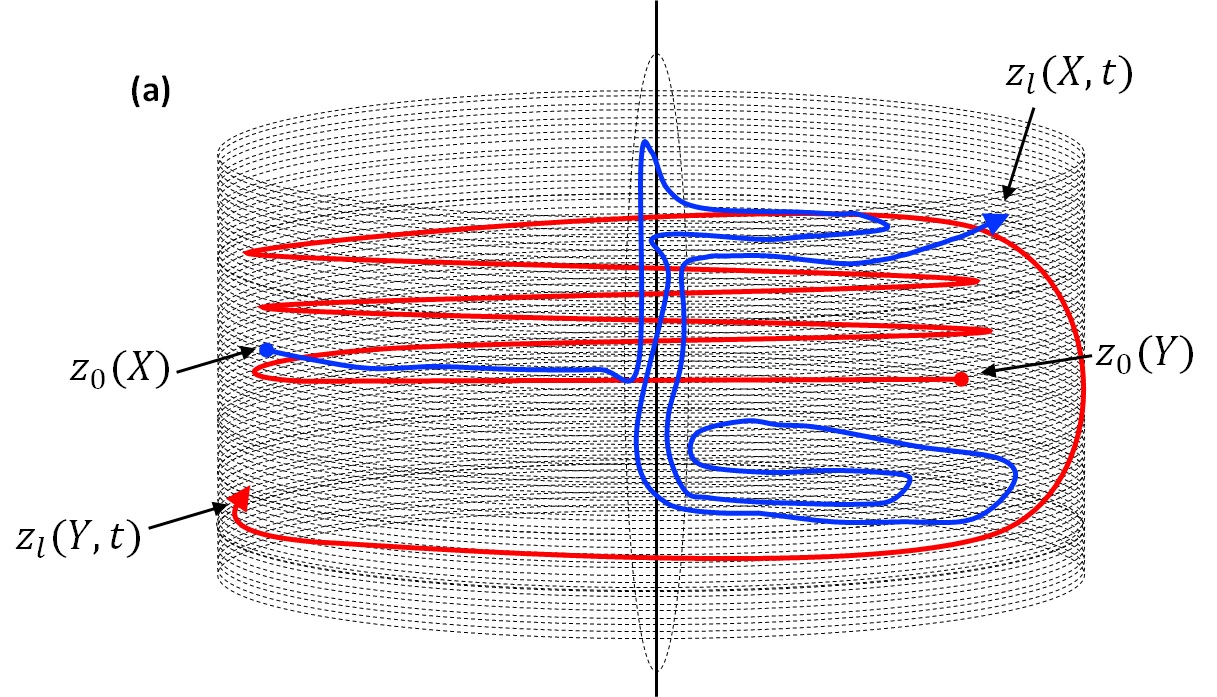
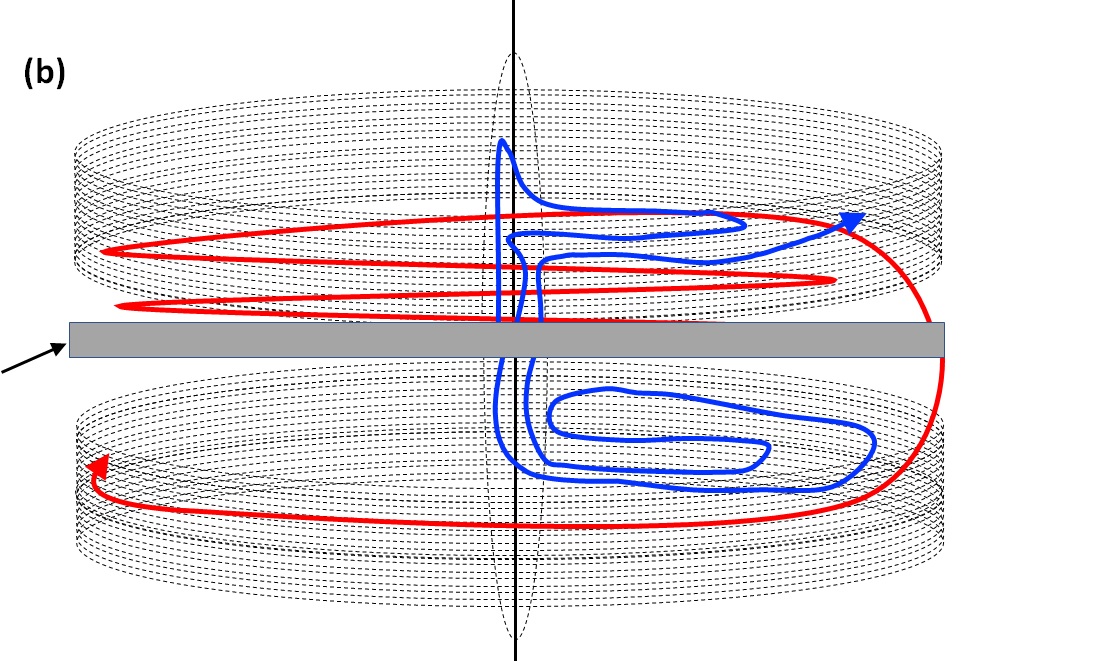
Figure 4.4. (a) Formation of contours in a bundle, and (b) formation of a hole in the bundle due to a removal process of an arbitrary plane in which contours originated.

4.2. PDE’s for the Dynamics of Lost Space

Suppose we consider simultaneously another arbitrary random variable $X^{b}\left(z_{l}(t),\mathbb{C}_{l}\right)$ along with $X^{a}\left(z_{l}(t),\mathbb{C}_{l}\right)$ in $\mathbb{C}_{l}$. As in $X^{b}\left(z_{l}(t),\mathbb{C}_{l}\right)$, we will develop two models, one for understanding the dynamics of the space lost by first assuming that $\gamma_{l}(X^{b},t)$ at $t=t_{c}$ is active in $B_{\mathbb{R}}(\mathbb{C},\alpha_{2})$ and then second time by assuming $\gamma_{l}(X^{b},t)$ at $t=t_{c}$ is active in $B_{\mathbb{R}}(\mathbb{C},1-\alpha_{2})$. When $\gamma_{l}(X^{b},t)$ at $t=t_{c}$ is active in $B_{\mathbb{R}}(\mathbb{C},\alpha_{2})$, the set of points touched by the contour $\gamma_{l}(X^{b},t)$ prior to $t_{c}$ would have located in $B_{\mathbb{R}}(\mathbb{C},\alpha_{2})$, $\mathbb{C}_{l}$, and $B_{\mathbb{R}}(\mathbb{C},1-\alpha_{2}).$ The contour $\gamma_{l}(X^{b},t)$ is described by $z_{l}(X^{b},t)$ $\left(t\in[t_{0},\infty)\right)$ and $t=O_{l_{c}}(X^{b},\tau,\alpha_{2})$ $\left(b_{0}\leq\tau\leq b{}_{c}\right)$ is the parametric representation for $\gamma_{l}(X^{b},t,\alpha_{2})$ with a real values function $O_{l_{c}}(X^{b},\tau,\alpha_{2})$ mapping $[b_{0},b_{c}]$ onto the interval $[t_{0},t_{c}].$ Let $L\left(\gamma_{l}(X^{b},t,\alpha_{2})\left(t\in[t_{0},t_{c}]\right)\right)$ represent the length of $\gamma_{l}(X^{b},t,\alpha_{2})\left(t\in[t_{0},t_{c}]\right)$ up to $t_{c},$ then

$$L\left(\gamma_{l}(X^{b},t,\alpha_{2})\left(t\in[t_{0},t_{c}]\right)\right)=\int_{b_{0}}^{b_{c}}\left|z[O_{l_{c}}(X^{b},\tau,\alpha_{2})]\right|O^{\prime}_{l_{c}}(X^{b},\tau,\alpha_{2})d\tau.$$

By following the procedure explained in section 4.1, we partition

$$L\left(\gamma_{l}(X^{b},t,\alpha_{2})\left(t\in[t_{0},t_{c}]\right)\right)$$

into a sum of three parts of piecewise contour lengths. The final differential equation to model the space of points lost due to only the removal process $\phi(X^{b},t,1-\alpha_{2})$ is

$$\left.\frac{dB_{\mathbb{R}}(\mathbb{C},1-\alpha_{2})}{dt}\right|_{\phi(X^{b},t,1-\alpha_{2})} =\left.B_{\mathbb{R}}(\mathbb{C},1-\alpha_{2})\right|_{t=t_{c}}-$$

(4.47) $$=\phi(X^{b},t,1-\alpha_{2})\left.B_{\mathbb{R}}(\mathbb{C},1-\alpha_{2})\right|_{t=t_{c}}$$

where

$$\phi(X^{b},t,1-\alpha_{2})=\psi(X^{b},t,1-\alpha_{2})\times$$

$$\sum_{i\in B(1-\alpha_{2})}\int_{b(i)}^{b(i+1)}\left|z[O_{l_{b(i+1)}}(X^{b},\tau)]\right|O^{\prime}_{l_{b(i+1)}}(X^{b},\tau)d\tau\text{ $\left(t\in(t_{c},t_{c^{\prime}}]\right)$}.$$

for $0<\psi(X^{b},t,1-\alpha_{2})<1.$ Meaning of the set $B(1-\alpha_{2})$ and the procedure to obtain the integral in (LABEL:eq:4-50) are similar to corresponding model in (LABEL:eq:4-38). Alternatively, when $\gamma_{l}(X^{b},t)$ at $t=t_{c}$ is active in $B_{\mathbb{R}}(\mathbb{C},1-\alpha_{2})$, the set of points touched by the contour $\gamma_{l}(X^{b},t)$ prior to $t_{c}$ would have located in $B_{\mathbb{R}}(\mathbb{C},\alpha_{2})$, $\mathbb{C}_{l}$, and $B_{\mathbb{R}}(\mathbb{C},1-\alpha_{2}).$ The the contour $\gamma_{l}(X^{b},t)$ can be described by $z_{l}(X^{b},t)$ $\left(t\in[t_{0},\infty)\right)$ and $t=Q_{l_{c}}(X^{b},\tau,1-\alpha_{2})$ $\left(b^{\prime}_{0}\leq\tau\leq b^{\prime}{}_{c}\right)$ is the parametric representation for $\gamma_{l}(X^{b},t,1-\alpha_{2})$ with a real values function $Q_{l_{c}}(X^{b},\tau,1-\alpha_{2})$ mapping $[b^{\prime}_{0},b^{\prime}_{c}]$ onto the interval $[t_{0},t_{c}].$ Let $L\left(\gamma_{l}(X^{b},t,1-\alpha_{2})\left(t\in[t_{0},t_{c}]\right)\right)$ represent the length of $\gamma_{l}(X^{b},t,1-\alpha_{2})\left(t\in[t_{0},t_{c}]\right)$ up to $t_{c},$ then

(4.49) $$\begin{array}[]{c}L\left(\gamma_{l}(X^{b},t,1-\alpha_{2})\left(t\in[t_{0},t_{c}]\right)\right)=\\ \int_{b^{\prime}_{0}}^{b^{\prime}_{c}}\left|z[Q_{l_{c}}(X^{b},\tau,1-\alpha_{2})]\right|Q^{\prime}_{l_{c}}(X^{b},\tau,1-\alpha_{2})d\tau.\end{array}$$

By following the procedure explained in section 4.1, we partition

$$L\left(\gamma_{l}(X^{b},t,1-\alpha_{2})\left(t\in[t_{0},t_{c}]\right)\right)$$

into a sum of three parts of piecewise contour lengths. The corresponding differential equation to model the space of points lost due to only the removal process $\phi(X^{b},t,\alpha_{2})$ is

$$\left.\frac{dB_{\mathbb{R}}(\mathbb{C},\alpha_{2})}{dt}\right|_{\phi(X^{b},t,\alpha_{2})} =\left.B_{\mathbb{R}}(\mathbb{C},1-\alpha_{2})\right|_{t=t_{c}}-$$

(4.50) $$\phi(X^{b},t,\alpha_{2})\left.B_{\mathbb{R}}(\mathbb{C},1-\alpha_{2})\right|_{t=t_{c}}$$

where

$$\phi(X^{b},t,\alpha_{2})=\psi(X^{b},t,\alpha_{2})\times$$

$$\sum_{i\in B^{\prime}(1-\alpha_{2})}\int_{b^{\prime}(i)}^{b^{\prime}(i+1)}\left|z[Q_{l_{b(i+1)}}(X^{b},\tau)]\right|Q^{\prime}_{l_{b(i+1)}}(X^{b},\tau)d\tau\text{ $\left(t\in(t_{c},t_{c^{\prime}}]\right)$}.$$

for $0<\psi(X^{b},t,1-\alpha_{2})<1.$ The set $B^{\prime}(1-\alpha_{2})$ consists of piecewise contours in $B_{\mathbb{R}}(\mathbb{C},1-\alpha_{2})$ as described in section 4.1 and the procedure to obtain the integral in (LABEL:eq:4-53) are similar to corresponding model in (LABEL:eq:4-46). The differential equations (4.47) and (4.50) are good when the removal process of $X^{a}(z_{l}(t),t)$ was not introduced simultaneously. The differential equations (LABEL:eq:4-37) and (LABEL:eq:4-45) does not provide dynamics of lost spaces when the removal process of $X^{b}(z_{l}(t),t)$ was not introduced simultaneously. Under the simultaneous existence of the two contours $\gamma_{l}(X^{a},t)$ and $\gamma_{l}(X^{b},t)$, and the corresponding removal processes, we will have four situations. Suppose $\gamma_{l}(X^{a},t)$ and $\gamma_{l}(X^{b},t)$ are active in $B_{\mathbb{R}}(\mathbb{C},\alpha_{2})$ at $t=t_{c}$, then the partial differential equation describing the dynamics of removal of the spaces created by $\gamma_{l}(X^{a},t)$ and $\gamma_{l}(X^{b},t)$ in $B_{\mathbb{R}}(\mathbb{C},1-\alpha_{2})$ until $t_{c}$ are

$$\left.\frac{\partial^{2}B_{\mathbb{R}}(\mathbb{C},1-\alpha_{2})}{\partial X^{a}\partial t}\right|_{\phi(X^{a},t,1-\alpha_{2})} =\left.B_{\mathbb{R}}(\mathbb{C},1-\alpha_{2})\right|_{t=t_{c}}-$$

(4.52) $$\frac{\partial\phi(X^{a},t,1-\alpha_{2})\left[L(X^{a}+X^{b},1-\alpha_{2})\right]}{\partial X^{a}},$$

$$\left.\frac{\partial^{2}B_{\mathbb{R}}(\mathbb{C},1-\alpha_{2})}{\partial X^{b}\partial t}\right|_{\phi(X^{b},t,1-\alpha_{2})} =\left.B_{\mathbb{R}}(\mathbb{C},1-\alpha_{2})\right|_{t=t_{c}}-$$

(4.53) $$\frac{\partial\phi(X^{b},t,1-\alpha_{2})\left[L(X^{a}+X^{b},1-\alpha_{2})\right]}{\partial X^{b}},$$

for the removal rates $\phi(X^{a},t,1-\alpha_{2})$, $\phi(X^{b},t,1-\alpha_{2})$ and length of contour formed due to $\gamma_{l}(X^{a},t)$ and $\gamma_{l}(X^{b},t)$ in $B_{\mathbb{R}}(\mathbb{C},1-\alpha_{2})$ is $L(X^{a}+X^{b},1-\alpha_{2}).$ Suppose $\gamma_{l}(X^{a},t)$ is active in $B_{\mathbb{R}}(\mathbb{C},\alpha_{2})$ and $\gamma_{l}(X^{b},t)$ is active in $B_{\mathbb{R}}(\mathbb{C},1-\alpha_{2})$ at $t=t_{c}$, then the partial differential equations describing the dynamics of removal of the space created by $\gamma_{l}(X^{a},t)$ in $B_{\mathbb{R}}(\mathbb{C},1-\alpha_{2})$ and $\gamma_{l}(X^{b},t)$ in $B_{\mathbb{R}}(\mathbb{C},\alpha_{2})$ until $t_{c}$ are

$$\left.\frac{\partial^{2}B_{\mathbb{R}}(\mathbb{C},1-\alpha_{2})}{\partial X^{a}\partial t}\right|_{\phi(X^{a},t,1-\alpha_{2})} =\left.B_{\mathbb{R}}(\mathbb{C},1-\alpha_{2})\right|_{t=t_{c}}-$$

(4.54) $$\frac{\partial\phi(X^{a},t,1-\alpha_{2})\left[L(X^{a},1-\alpha_{2})+L(X^{b},\alpha_{2})\right]}{\partial X^{a}},$$

$$\left.\frac{\partial^{2}B_{\mathbb{R}}(\mathbb{C},\alpha_{2})}{\partial X^{b}\partial t}\right|_{\phi(X^{b},t,1-\alpha_{2})} =\left.B_{\mathbb{R}}(\mathbb{C},\alpha_{2})\right|_{t=t_{c}}-$$

(4.55) $$\frac{\partial\phi(X^{b},t,\alpha_{2})\left[L(X^{a},1-\alpha_{2})+L(X^{b},\alpha_{2})\right]}{\partial X^{a}},$$

where $\phi(X^{a},t,1-\alpha_{2})$ and $\phi(X^{b},t,\alpha_{2})$ are the removal rates of $\gamma_{l}(X^{a},t)$ and $\gamma_{l}(X^{b},t)$ in $B_{\mathbb{R}}(\mathbb{C},1-\alpha_{2})$, and $B_{\mathbb{R}}(\mathbb{C},\alpha_{2})$, respectively. The sum of the piecewise lengths in $B_{\mathbb{R}}(\mathbb{C},1-\alpha_{2})$, and $B_{\mathbb{R}}(\mathbb{C},\alpha_{2})$ are represented by $L(X^{a},1-\alpha_{2})$ and $L(X^{b},\alpha_{2}),$ respectively. Suppose $\gamma_{l}(X^{a},t)$ and $\gamma_{l}(X^{b},t)$ are active in $B_{\mathbb{R}}(\mathbb{C},1-\alpha_{2})$ at $t=t_{c}$, then the partial differential equation describing the dynamics of removal of the spaces created by $\gamma_{l}(X^{a},t)$ and $\gamma_{l}(X^{b},t)$ in $B_{\mathbb{R}}(\mathbb{C},\alpha_{2})$ until $t_{c}$ are

$$\left.\frac{\partial^{2}B_{\mathbb{R}}(\mathbb{C},\alpha_{2})}{\partial X^{a}\partial t}\right|_{\phi(X^{a},t,\alpha_{2})} =\left.B_{\mathbb{R}}(\mathbb{C},\alpha_{2})\right|_{t=t_{c}}-$$

(4.56) $$\frac{\partial\phi(X^{a},t,\alpha_{2})\left[L(X^{a}+X^{b},\alpha_{2})\right]}{\partial X^{a}},$$

$$\left.\frac{\partial^{2}B_{\mathbb{R}}(\mathbb{C},\alpha_{2})}{\partial X^{b}\partial t}\right|_{\phi(X^{b},t,\alpha_{2})} =\left.B_{\mathbb{R}}(\mathbb{C},\alpha_{2})\right|_{t=t_{c}}-$$

(4.57) $$\frac{\partial\phi(X^{b},t,\alpha_{2})\left[L(X^{a}+X^{b},\alpha_{2})\right]}{\partial X^{b}},$$

where $\phi(X^{a},t,\alpha_{2})$ and $\phi(X^{b},t,\alpha_{2})$ are the removal rates and the sums of the piecewise lengths of contours formed due to $\gamma_{l}(X^{a},t)$ and $\gamma_{l}(X^{b},t)$ in $B_{\mathbb{R}}(\mathbb{C},\alpha_{2})$ is $L(X^{a}+X^{b},\alpha_{2}).$ Suppose $\gamma_{l}(X^{a},t)$ is active in $B_{\mathbb{R}}(\mathbb{C},1-\alpha_{2})$ and $\gamma_{l}(X^{b},t)$ is active in $B_{\mathbb{R}}(\mathbb{C},\alpha_{2})$ at $t=t_{c}$, then the partial differential equations describing the dynamics of removal of the space created by $\gamma_{l}(X^{a},t)$ in $B_{\mathbb{R}}(\mathbb{C},\alpha_{2})$ and $\gamma_{l}(X^{b},t)$ in $B_{\mathbb{R}}(\mathbb{C},1-\alpha_{2})$ until $t_{c}$ are

$$\left.\frac{\partial^{2}B_{\mathbb{R}}(\mathbb{C},\alpha_{2})}{\partial X^{a}\partial t}\right|_{\phi(X^{a},t,\alpha_{2})} =\left.B_{\mathbb{R}}(\mathbb{C},\alpha_{2})\right|_{t=t_{c}}-$$

(4.58) $$\frac{\partial\phi(X^{a},t,\alpha_{2})\left[L(X^{a},\alpha_{2})+L(X^{b},1-\alpha_{2})\right]}{\partial X^{a}},$$

$$\left.\frac{\partial^{2}B_{\mathbb{R}}(\mathbb{C},1-\alpha_{2})}{\partial X^{b}\partial t}\right|_{\phi(X^{b},t,1-\alpha_{2})} =\left.B_{\mathbb{R}}(\mathbb{C},1-\alpha_{2})\right|_{t=t_{c}}-$$

(4.59) $$\frac{\partial\phi(X^{b},t,\alpha_{2})\left[L(X^{a},\alpha_{2})+L(X^{b},1-\alpha_{2})\right]}{\partial X^{a}},$$

where $\phi(X^{a},t,\alpha_{2})$ and $\phi(X^{b},t,1-\alpha_{2})$ are the removal rates of $\gamma_{l}(X^{a},t)$ and $\gamma_{l}(X^{b},t)$ in $B_{\mathbb{R}}(\mathbb{C},\alpha_{2})$, and $B_{\mathbb{R}}(\mathbb{C},1-\alpha_{2})$, respectively. The sum of the piecewise lengths in $B_{\mathbb{R}}(\mathbb{C},\alpha_{2})$, and $B_{\mathbb{R}}(\mathbb{C},1-\alpha_{2})$ are represented by $L(X^{a},\alpha_{2})$ and $L(X^{b},1-\alpha_{2}),$ respectively. The two partitions in $B_{\mathbb{R}}(\mathbb{C},\alpha_{2})$, and $B_{\mathbb{R}}(\mathbb{C},1-\alpha_{2})$ behave independently in terms of further removal and growth of contours.

The PDEs represented in (4.52) through (4.59) are simultaneous removal of two contours at a time. These can be treated as an example of the removal process of the dynamics of multiple removal processes. The plan is to remove all the infinitely many contours at $t_{c}$.

5. Concluding Remarks

Multilevel contours passing through bundle $B_{\mathbb{R}}(\mathbb{C})$ of complex planes could demonstrate interesting properties. The random environment created brings the dynamic nature of the bundle through the removal process introduced. The continuous-time Markov properties, differential equations, and topological analysis on the bundle give scope to further investigate them using functional approximations. The transportation of information through contours for different complex planes could be extended further for practical situations arising out of transportation problems. There are several applications of complex analysis that are out of scope to discuss in this article. A wide range of literature is available for interested readers, see for example [5, 11, 12, 13, 14, 15, 16]. One can also introduce several forms of parametric contour formations by assuming functional growth rates of contours. That could be an independent approach towards modeling the behavior of the contours concerning a given functional form of contour formation. Similarly, the removal rates can be assumed to follow certain closed-form approximations (special forms of Harmonic functions, and Poisson integrals). Information carried between various complex planes that were discussed in Section 2 would be obstructed if the set of points that a given connected contour gets deleted (lost) due to a removal process.

References

- [1] Ahlfors, Lars V. Complex analysis. An introduction to the theory of analytic functions of one complex variable. Third edition. International Series in Pure and Applied Mathematics. McGraw-Hill Book Co., New York, 1978. xi+331
- [2] Churchill, Ruel V.; Brown, James Ward Complex variables and applications. Fourth edition. McGraw-Hill Book Co., New York, 1984. x+339 pp.
- [3] Krantz, Steven G. Complex analysis: the geometric viewpoint. Second edition. Carus Mathematical Monographs, 23. Mathematical Association of America, Washington, DC, 2004. xviii+219 pp.
- [4] Rudin, Walter Real and complex analysis. Third edition. McGraw-Hill Book Co., New York, 1987. xiv+416 pp. ISBN: 0-07-054234-1
- [5] Rao A.S.R.S. and Krantz S.G. (2021). Rao distances and conformal mappings, Information Geometry, Volume 45: Handbook of Statistics, Elsevier/North-Holland, Amsterdam
- [6] Good, I. J. The frequency count of a Markov chain and the transition to continuous time. Ann. Math. Statist. 32 (1961), 41–48.
- [7] Bhat, B. R.; Deshpande, Sunita K. Likelihood ratio test for testing order of continuous time finite Markov chains. Comm. Statist. A—Theory Methods 15 (1986), no. 6, 1751–1771.
- [8] Chen, Mu Fa On three classical problems for Markov chains with continuous time parameters. J. Appl. Probab. 28 (1991), no. 2, 305–320.
- [9] Gani, J.; Stals, L. A continuous time Markov chain model for a plantation-nursery system. Environmetrics 16 (2005), no. 8, 849–861.
- [10] Goswami, A.; Rao, B. V. A course in applied stochastic processes. Texts and Readings in Mathematics, 40. Hindustan Book Agency, New Delhi, 2006.
- [11] Sagun Chanillo, Paulo D. Cordaro, Nicholas Hanges, Jorge Hounie and Abdelhamid Meziani (Edited). Geometric analysis of PDE and several complex variables. Dedicated to Franï¿œois Treves. Including papers from the workshop held in Sï¿œo Paulo, August 2003.. Contemporary Mathematics, 368. American Mathematical Society, Providence, RI, 2005
- [12] Ponnusamy, S.; Silverman, Herb Complex variables with applications. Birkhï¿œuser Boston, Inc., Boston, MA, 2006.
- [13] Campos, L. M. B. C. Complex analysis with applications to flows and fields. Mathematics and Physics for Science and Technology. CRC Press, Boca Raton, FL, 2011.
- [14] Pathak, H.K. Complex analysis and applications. Springer, Singapore, 2019
- [15] Cohen, Harold Complex analysis with applications in science and engineering. Second edition. Springer, New York, 2007.
- [16] Krantz, Steven G. Complex variables. A physical approach with applications and MATLABᅵ. Textbooks in Mathematics. Chapman & Hall/CRC, Boca Raton, FL, 2008.