Structure-aware Interactive Graph Neural Networks
for the Prediction of Protein-Ligand Binding Affinity

Abstract.

Drug discovery often relies on the successful prediction of protein-ligand binding affinity. Recent advances have shown great promise in applying graph neural networks (GNNs) for better affinity prediction by learning the representations of protein-ligand complexes. However, existing solutions usually treat protein-ligand complexes as topological graph data, thus the biomolecular structural information is not fully utilized. The essential long-range interactions among atoms are also neglected in GNN models. To this end, we propose a structure-aware interactive graph neural network (SIGN) which consists of two components: polar-inspired graph attention layers (PGAL) and pairwise interactive pooling (PiPool). Specifically, PGAL iteratively performs the node-edge aggregation process to update embeddings of nodes and edges while preserving the distance and angle information among atoms. Then, PiPool is adopted to gather interactive edges with a subsequent reconstruction loss to reflect the global interactions. Exhaustive experimental study on two benchmarks verifies the superiority of SIGN.

1. Introduction

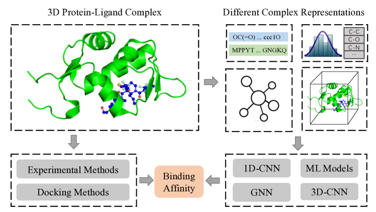
Figure 1. A brief summary for protein-ligand binding affinity prediction. (1) Top left: An example of protein-ligand complex (PDB: 5HMI). (2) Top right: Various representations of complex. (3) Bottom left: Traditional Methods. (4) Bottom right: Machine learning and deep learning methods.

The prediction of protein-ligand binding affinity has been widely considered as one of the most important tasks in computational drug discovery (Kitchen et al., 2004). Here ligands are usually drug candidates including small molecules and biologics which can interact with proteins as agonists or inhibitors in the biological processes to cure diseases. The binding affinity, defined as the strength of the binding interaction between a protein and a ligand (e.g., drug), can be measured by experimental methods. However, those biological tests are laborious and time-consuming. With the computer aided simulation methods and the data-driven learning models, binding affinities can be predicted in the early stage of drug discovery. Instead of applying costly biological methods directly to screen numerous candidate molecules, the prediction of binding affinity can help to rank drug candidates and prioritize the appropriate ones for subsequent testing to accelerate the process of drug screening (Li and Shah, 2017).

With the development of structural biology and protein structure prediction, especially the recent Alphafold II model (Callaway, 2020), there are growing three-dimensional (3D) structure protein data, which enables a new paradigm for structure-based drug discovery (Jhoti and Leach, 2007; Meng et al., 2011; Batool et al., 2019). It has been demonstrated that 3D structural information can effectively contribute to the drug design (Leach et al., 2006). Indeed, since there are already many accurate and robust algorithms to find poses of protein-ligand complexes (e.g., binding site prediction methods and docking methods), it is significant to focus on the much harder task of binding affinity prediction (Ballester and Mitchell, 2010). To learn useful 3D structure from a protein-ligand complex, as illustrated in Figure 1, many efforts have been devoted to estimating more accurate binding affinity for effective drug design. Docking methods (Jain, 2003; Trott and Olson, 2010; Allen et al., 2015) play an important role to predict how a specific ligand binds to the target protein with affordable computational costs. While the docking process can identify the binding pose of the protein-ligand complex with relatively high accuracy, its prediction of binding affinity is inaccurate and unreliable (Moitessier et al., 2008; Ballester and Mitchell, 2010) due to poor scoring functions, which limits the applicability of docking methods in drug discovery. Compared to docking calculations, traditional machine learning methods (Ballester and Mitchell, 2010; Kinnings et al., 2011) have improved the performance by learning the extracted features from protein-ligand complexes. However, these approaches with limited generalizability require expert knowledge and heavily rely on feature engineering.

Recently, deep learning for binding affinity prediction have become an emerging research area, which represents the complex as sequence data (Öztürk et al., 2018), 3D grid-like data (Wallach et al., 2015) or graph data (Nguyen et al., 2020) to employ various neural networks. One of the key challenges of deep learning in structural biology is how to model the 3D spatial structure for better performance. To this end, most of the existing works (Wallach et al., 2015; Ragoza et al., 2017; Stepniewska-Dziubinska et al., 2018) attempt to apply 3D convolutional neural networks (3D CNNs) by treating the complex as a 3D-grid representation. However, the cost of these models is huge, especially when considering long-range interactions. What’s more, both the absence of topological information and the sensitivity to rotation in the complex have a negative effect on the prediction results.

Despite the powerful ability of graph neural networks (GNNs) to learn graph representations (Li et al., 2020; Zheng et al., 2021; Liu et al., 2021), there are only a few studies (Lim et al., 2019; Nguyen et al., 2020) on using GNNs to predict the protein-ligand binding affinity. By contrast, many researchers have greatly developed GNN models in other fields of drug discovery (Sun et al., 2020; Zang and Wang, 2020), such as predicting molecular property (Yang et al., 2019; Maziarka et al., 2020; Klicpera et al., 2020) and chemical reaction (Do et al., 2019). Nevertheless, these domain-specific models tend to lose their effectiveness when modeling the larger biomolecules, e.g., protein-ligand complexes. In general, most of the existing GNNs in drug design aim to learn the spatial structure by incorporating the distance information, which is insufficient to model the 3D structure of complex. Moreover, the fundamental long-range interactive information between proteins and ligands, which is valuable for predicting the binding affinity (Leckband et al., 1992), cannot be handled under the current GNN framework.

To overcome the above limitations, we propose a novel Structure-aware Interactive Graph Neural Network (SIGN) to learn the constructed complex graph for predicting the protein-ligand binding affinity. SIGN is equipped with two designed components to correspondingly address the challenges, namely the polar-inspired graph attention layers (PGAL) for modeling 3D spatial structure and the pairwise interactive pooling (PiPool) for leveraging long-range interactions. Firstly, the key idea of PGAL is to establish a polar coordinate system for each central target and to preserve both distance and angle information of neighbors when performing the aggregation process. More specifically, we apply the node-edge interactive scheme iteratively with graph attention to integrate spatial factors for effectively learning the 3D structure of complex.

In view of the large size of the protein, it is redundant to contain the complete protein structure in the complex graph, but in this way the long-range interactive information between the protein and the ligand is also lost. To deal with this issue, PiPool, the secondary part of SIGN is designed to incorporate such global interactions into our model, which employs an atomic type-aware pooling process on edges with introducing an auxiliary learning task to reconstruct the atomic interaction matrix. By this means, SIGN can enhance the representation learning for complexes with involving both 3D spatial structures and global interactions. To summarize, the main contributions of this paper are as follows:

• To the best of our knowledge, we are among the first to develop graph neural networks from the perspective of polar coordinates for structure-based binding affinity prediction.

• We propose a novel structure-aware interactive graph neural network (SIGN), which can capture not only 3D spatial information through polar-inspired graph attention layers (PGAL), but also global long-range interactions through pairwise interactive pooling (PiPool) in a semi-supervised manner.

• We conduct extensive experiments using two benchmark datasets to evaluate the performance of the proposed model, which demonstrates the effectiveness of our SIGN with better generalizability.

2. Related Work

In this section, we first review the related literatures about predicting protein-ligand binding affinity and then detail recent advances in graph neural networks for drug discovery.

Protein-Ligand Binding Affinity Prediction. As a crucial stage in drug discovery, predicting protein-ligand binding affinity has been intensively studied for a long time (Sousa et al., 2006; Jacob and Vert, 2008), which is of great importance for efficient and accurate drug screening. The earlier empirical-based methods (Gohlke et al., 2000; Wang et al., 2002; Trott and Olson, 2010) design docking and scoring functions specially to make predictions, while expert domain knowledge is required to encode internal biochemical interactions. Later on, statistical and machine learning-based methods (Colwell, 2018) are developed to predict binding affinity based on data-driven learning, which attempt to extract protein-ligand features and use classic models for regression, such as random forest (Ballester and Mitchell, 2010) and SVM (Kinnings et al., 2011). These approaches are dependent on the quality of hand-crafted features and lack of generality on the larger dataset. Recently, several deep learning-based models (Öztürk et al., 2018) utilize 1D convolutions and pooling to capture potential patterns from raw sequence information of both ligand and protein. However, only using separate character representations fails to achieve desirable performance.

With the recent advances in predicting structures of proteins (Callaway, 2020) and the increasing availability of 3D-structure protein-ligand data (Wang et al., 2005), there is another hot research area of studying structure-based approaches, which focus on learning from 3D-structure protein-ligand complexes to predict binding affinity. Some recent works (Ragoza et al., 2017; Stepniewska-Dziubinska et al., 2018) represent the protein-ligand complex as 3D grid-like data and use 3D convolutions (3D-CNNs) to take advantage of spatially-local correlations. Though these approaches can learn spatial information, one limitation is that positions of proteins and ligands in different complexes are changeable, such as different angle rotations, which means the spatial structure of 3D grid-like modeling is inevitably incomplete. More recently, OnionNet (Zheng et al., 2019) employs CNN models to learn the complex representation from the extracted element-specific interaction features between a protein and its ligand. However, all the above models neglect the critical topological structure information of complex. In the work (Lim et al., 2019), a protein-ligand complex is represented as a weighted graph with distance information. Then graph attention networks are applied to predicting the interactions. Nevertheless, only distance information between atoms is not adequate to model 3D-structure interactions. In this paper, we also focus on the structure-based prediction of protein-ligand binding affinity with incorporating abundant spatial information.

Graph Neural Networks for Drug Discovery. Inspired by the great advantage of graph neural networks (GNNs) in modeling graph data, much attention has been devoted to applying them in computational drug discovery (Sun et al., 2020), such as the prediction of molecular property (Hao et al., 2020) and protein interface (Liu et al., 2020). Treating the molecule as a graph, GNNs can learn the graph-level representation for drug or protein by aggregating structural information. GraphDTA (Nguyen et al., 2020) adopts GNN models (Kipf and Welling, 2017; Veličković et al., 2018; Xu et al., 2019) to learn drug presentation with combining the protein representation from 1D convolutions to predict binding affinity. In attributed molecular graphs, the edges between atoms contain valuable information, such as distance or bond order. To leverage rich attributes in the molecule, edge-oriented message passing neural networks (Yang et al., 2019; Song et al., 2020; Zhou et al., 2020) are proposed to update both node and edge embeddings . Meanwhile, there are also some efforts to model the 3D-structure of molecule by improving GNNs with spatial information, such as distance (Lim et al., 2019; Maziarka et al., 2020), angle (Klicpera et al., 2020), and 3D coordinate (Danel et al., 2020). However, these models fail to consider the spatial interactions between proteins and ligands. In addition, the function of learning angle information in (Klicpera et al., 2020) is designed for density functional theory, which is only beneficial for predicting molecular properties rather than protein-ligand binding affinity. To overcome these limitations, we propose an interaction-aware GNN framework with integrating both distance and angle factors harmoniously.

3. Preliminaries

In this section, we introduce some definitions used in our model and formulate the structure-based prediction problem for protein-ligand binding affinity. The frequently used notations in this paper are summarized in Table 1.

Table 1. Mathematical notations.

Notation	Description
$\mathcal{V}^{P}$,$\mathcal{V}^{L}$	The atom node sets of protein and ligand
$M^{P}$,$M^{L}$	The 3D position matrices of protein and ligand
$\mathcal{G}_{I}$	The complex interaction graph
$a_{i}$	The $i$-th atom node in $\mathcal{G}_{I}$
$e_{ij}$	The directed edge from atom $a_{i}$ to atom $a_{j}$
$\mathcal{N}_{e}(a_{i})$	The neighboring edges of atom $a_{i}$
$\mathcal{N}_{e}(e_{ij})$	The neighboring edges of edge $e_{ij}$
$\bm{a}_{i}$, $\bm{e}_{ij}$	The embedding vectors of atom $a_{i}$ and edge $e_{ij}$
$\bm{d}_{ij}$	The spatial embedding vector between $a_{i}$ and $a_{j}$

Figure 2. An illustrative example of converting the protein-ligand complex into a complex interaction graph.

Definition 3.1.

Complex Interaction Graph. Given a protein-ligand complex as shown in Figure 2(a), we define the atom node sets of protein and ligand as $\mathcal{V}^{P}=\{a^{P}_{1},...,a^{P}_{m}\}$ and $\mathcal{V}^{L}=\{a^{L}_{1},...,a^{L}_{n}\}$ with the position matrix $M^{P}\in\mathbb{R}^{m\times 3}$ and $M^{L}\in\mathbb{R}^{n\times 3}$ for 3D atomic coordinates, respectively. Then we define the complex interaction graph as a directional graph $\mathcal{G}_{I}=<\mathcal{V},\mathcal{E}>$, where the vertex set $\mathcal{V}\subseteq\mathcal{V}^{P}\cup\mathcal{V}^{L}$ and the edge set $\mathcal{E}=f_{e}(\mathcal{V}^{P},\mathcal{V}^{L},M^{P},M^{L})$ are constructed based on the spatial positions of atoms. The graph construction process is introduced in Appendix A.1.

Definition 3.2.

Edge-oriented Neighbors. Given an atom node $a_{i}$ or a directed edge $e_{ij}$ (i.e., $a_{i}\rightarrow a_{j}$) in the complex interaction graph $\mathcal{G}_{I}$, the edge-oriented neighbors $\mathcal{N}_{e}$ of $a_{i}$ or $e_{ij}$ are defined as the sets of directed edges $\{e_{ki},...,e_{li}\}$ which point to the target atom $a_{i}$ or the target edge $e_{ij}$.

Taking Figure 2(b) as an example, the edges $e_{21}$ and $e_{41}$ are connected to the edge $e_{13}$ via the common node $a_{1}$, the edge-oriented neighbors of $e_{13}$ are denoted as $\mathcal{N}_{e}(e_{13})=\{e_{21},e_{41}\}$. Similarly, the edges $e_{13}$, $e_{53}$ and $e_{63}$ point to the atom node $a_{3}$, resulting in the neighbors set $\mathcal{N}_{e}(a_{3})=\{e_{13},e_{53},e_{63}\}$.

Definition 3.3.

Structure-based Protein-Ligand Binding Affinity Prediction. Given a protein-ligand complex with 3D structure, i.e., the complex interaction graph $\mathcal{G}_{I}$ and the 3D position matrix $M$ consisting of $M^{P}$and $M^{L}$, our goal is to learn a model $f:(\mathcal{G}_{I}|M)\rightarrow y$ to precisely predict the binding affinity $y$ with preserving the spatial structure.

4. Model Framework

(a) All edges

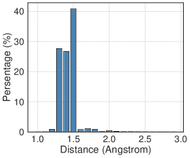
(b) Single bonds

(c) Double bonds

Figure 3. The distribution of distance between atoms within 5 Å in the protein-ligand complex from PDBbind dataset.

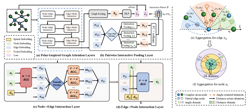
Figure 4. Illustration of the proposed SIGN framework. (a), (b): The two key components PGAL and PiPool. (c), (d): The two inner structures of component PGAL. (e), (f): The aggregation processes in node$\rightarrow$edge and edge$\rightarrow$node interaction layers.

In this section, we present the proposed SIGN model for protein-ligand binding affinity prediction. We first introduce the overall framework and then describe the details of each component.

4.1. Overview

To make accurate predictions for protein-ligand binding affinity, there are two challenges. Firstly, as shown in Figure 2, the complex graph has the unique spatial structure, which is different with general graph. Secondly, the long-range interactions between protein and ligand are also critical to the binding affinity (Leckband et al., 1992). However, the existing GNNs are incapable of capturing such spatial information and interactions. To overcome the limitations, we propose a novel Structure-aware Interactive Graph Neural Network (SIGN) to model the 3D structural complex and protein-ligand spatial interactions.

Figure 4 exhibits the architecture which takes the complex interaction graph $\mathcal{G}_{I}$ as input. We start with the polar-inspired graph attention layers (PGAL), which are composed of node$\rightarrow$edge and edge$\rightarrow$node interaction layers. PGAL can propagate the node’s and edge’s embeddings alternately with learning the spatial distance and angle information. The two parts of PGAL play a synergistic effect on modeling the spatial structure of the complex. After that, we apply a pairwise interactive pooling layer (PiPool) which performs on the edges’ representations to obtain the atomic type-based interaction matrix of the complex. From a global view, PiPool aims to approximate the overall interactions between proteins and ligands to improve the prediction performance. Finally, the model is trained through multi-task learning with augmented constraints for the interaction matrix, which serves as a self-supervised task.

4.2. Polar Coordinate-Inspired Graph Attention

Standard GNNs have shown great advantages in learning topological structure of the general graph, which cannot take atom’s spatial position into account in the 3-dimensional space. To model the 3D structure of a complex, an intuitive method is to provide atom’s 3-dimensional coordinate in the GNN architecture (Danel et al., 2020). However, the position information under the Cartesian coordinate system is sensitive to both translations and rotations, causing poor generalization of model when learning the complex representation. Several models, such as GNN-DTI (Klicpera et al., 2020) and MAT (Maziarka et al., 2020), manage to combine the distance information in the aggregation process, while only pairwise distance is not adequate. Different from DimeNet (Klicpera et al., 2020), which specially designs Bessel functions in GNN for density functional theory (DFT) approximation with limited ability to model the larger biological complex, we employ iterative node$\rightarrow$edge and edge$\rightarrow$node interaction layers to incorporate both distance and angle information from a spatial distribution perspective.

4.2.1. Polar-Inspired Attentive Learning Architecture.

Inspired by polar coordinate which is composed of radial distance $r$ and polar angle $\phi$, we develop an interaction-based graph attention network to leverage both the distance between nodes and the angle between edges in a collaborative framework. As illustrated in Figure 4(e), when aggregating for edge $e_{ij}$, we treat it as the polar axis $L$. Under such a definite polar coordinate system, the edge-oriented neighbors are distributed around $e_{ij}$ with unique identifying coordinates $(r,\phi)$. Through the method of dividing angle domains, the spatial distribution for the complex can be taken into account by means of angle-oriented attention in the first aggregation stage for edges.

Moreover, the distance factor is also helpful for structure modeling, which reveals spatial correlations. Figure 3 shows the statistical distribution of distance between atoms. It can be seen that the distances of covalent bonds mainly range from 1 to 2 Å, while noncovalent interactions, like hydrophobic and van der Waals interactions, and hydrogen bonds, are distributed over longer distances. Atomic interactions in the complex vary from different distances, which indicate different spatial relations for atom pairs. Given the radial distance $r$ between atoms $a_{i}$ and $a_{j}$, as shown in Figure 4(f), we first map $r$ to a bucket (i.e., a distance domain corresponding to a type of relation) and obtain the one-hot vector $\bm{x}_{ij}$. Then we apply a dense layer transformation to get the spatial relation embedding:

(1) $$\bm{d}_{ij}=\bm{W}_{s}\bm{x}_{ij},$$

where $\bm{W}_{s}\in\mathbb{R}^{d_{s}\times b}$ is the transformation weight matrix and $b$ is the number of buckets (i.e., spatial relations). To factor in these correlations, we design the distance-aware attention in the second aggregation stage for nodes. As shown in Figure 4(a), the overall attentive interaction process at $l$-th layer is defined as:

(2) $$\bm{e}_{ij}^{(l)} =f^{(l)}\Big{(}\big{\{}(\bm{a}_{k}^{(l-1)},\bm{a}_{i}^{(l-1)}),\forall e_{ki}\in\mathcal{N}_{e}(e_{ij})\big{\}}\Big{)},$$

(3) $$\bm{a}_{j}^{(l)} =g^{(l)}\Big{(}\bm{a}_{j}^{(l-1)},\big{\{}\bm{e}_{kj}^{(l)},\forall e_{kj}\in\mathcal{N}_{e}(a_{j})\big{\}}\Big{)},$$

where $\bm{e}_{ij}^{(l)}$ is the edge embedding, $\bm{a}_{j}^{(l)}$ is the node (atom) embedding, $f(\cdot)$ and $g(\cdot)$ are interaction functions of node$\rightarrow$edge and edge$\rightarrow$node layers, $\mathcal{N}_{e}(e_{ij})$ and $\mathcal{N}_{e}(a_{j})$ are the edge-oriented neighbors of edge $e_{ij}$ and node $a_{j}$ respectively.

4.2.2. Angle-oriented Node$\rightarrow$Edge Interaction Layer.

Failing to distinguish neighbor nodes from different directions in the aggregation process is a weakness of the existing GNN models. To overcome this inadequacy, we adopt an angle-oriented graph attention layer to update the edge representations with integrating spatial angle information. Since the angle exists between the two edges, as shown in Figure 4(c), we first get the edge embedding through aggregating the node features:

(4) $$\bm{e}_{ij}^{(l)}=\sigma(\bm{W}_{a\rightarrow e}^{(l)}\cdot[\bm{a}_{i}^{(l-1)}\mathbin{\|}\bm{a}_{j}^{(l-1)}\mathbin{\|}\bm{d}_{ij}]),$$

where $\bm{W}_{a\rightarrow e}^{(l)}$ is the transformation matrix for atomic combination, the operator $\mathbin{\|}$ represents concatenation, and $\sigma$ is the Relu function.

After obtaining the representations $\{\bm{e}_{ij}^{(l)},\bm{e}_{ki}^{(l)},..,\bm{e}_{mi}^{(l)}\}$ of edge $e_{ij}$ and its neighbors, we further separate the neighboring edges in 3-dimensional space by applying an angle-domain divider $\bm{D_{A}}$, which plays an intermediate role to assign each neighbor to the specific angle domain. For example, in Figure 4(e), there are four edge-oriented neighbors $e_{1i},e_{2i},e_{3i}$ and $e_{4i}$ around the central target edge $e_{ij}$. These neighboring edges are located in three different local angle domains according to the angles between edge $e_{ij}$ and its neighbors. Given the number of angle domains $N$ (e.g., $N=3$ in Figure 4(e)) and the target edge $e_{ij}$ for aggregation, $\bm{D_{A}}$  can map each neighbor $e_{ki}$ to the located angle domain index:

(5) $$Ind_{ki}=\bm{D_{A}}(e_{ki},e_{ij},N)=\lceil N\cdot\frac{\phi_{kij}}{180}\rceil,$$

where $\lceil\cdot\rceil$ denotes rounding operation to get the integer index, $\phi_{kij}\in[0,180^{\circ}]$ is the calculated angle between edges $e_{ki}$ and $e_{ij}$. Then the subset of edge-oriented neighbors which are located in $q$-th angle domain can be defined as:

(6) $$\mathcal{N}^{q}_{e}(e_{ij})=\{e_{ki}\ |\ e_{ki}\in\mathcal{N}_{e}(e_{ij})\land Ind_{ki}=q\}.$$

After reorganizing the neighbors of $e_{ij}$ through divider $\bm{D_{A}}$  based on the polar coordinate system, we then feed $N$ neighbor subsets from different angle domains into $N$ independent propagation layers to capture long-range dependencies in the complex interaction graph. Firstly, we devise the domain-specific aggregation process along edges for the $q$-th angle domain:

(7) $$\bm{m}^{(l)}_{ij,q}=\sum_{e_{ki}\in\mathcal{N}^{q}_{e}(e_{ij})}\alpha^{(l)}_{ki,q}\cdot\bm{e}^{(l)}_{ki},\ \ \ 1\leq q\leq N,$$

where $\bm{m}^{(l)}_{ij,q}$ is the $q$-th local aggregated edge representation at $l$-th layer, $\alpha^{(l)}_{ki,q}$ is the attention weight of the neighboring edge $e_{ki}$ across the $q$-th angle domain. Concretely, we apply the angle-oriented attention mechanism, which first uses $attn_{q}^{l}$ function to calculate the coefficient between two edges and then adopts the softmax function for normalization:

(8) $$attn_{q}^{l}(e_{ij},e_{ki}) =\bm{u}^{T}_{l,q}\cdot tanh\big{(}\bm{W}^{(l)}_{e,q}\cdot[\bm{e}^{(l)}_{ij}\mathbin{\|}\bm{e}^{(l)}_{ki}]+\bm{b}^{(l)}_{e,q}\big{)},$$

(9) $$\alpha^{(l)}_{ki,q} =\frac{{\rm exp}\big{(}attn_{q}^{l}(e_{ij},e_{ki})\big{)}}{\sum_{e_{ti}\in\mathcal{N}^{q}_{e}(e_{ij})}{\rm exp}\big{(}attn_{q}^{l}(e_{ij},e_{ti})\big{)}},$$

where $\bm{u}_{l,q}$, $\bm{W}^{(l)}_{e,q}$ and $\bm{b}^{(l)}_{e,q}$ are the learnable attention parameters of the specific $q$-th angle domain, and we use tanh as the nonlinear activation function.

Secondly, we combine all aggregated edge embeddings obtained from Eq. (7). To completely preserve the spatial information in different local angle domains, we concatenate the representations as the global aggregation to update the angle-aware edge embedding:

(10) $$\bm{e}^{(l)}_{ij}=[\bm{m}^{(l)}_{ij,1}\mathbin{\|}\bm{m}^{(l)}_{ij,2}\mathbin{\|}\cdots\mathbin{\|}\bm{m}^{(l)}_{ij,N}].$$

4.2.3. Distance-aware Edge$\rightarrow$Node Interaction Layer.

After injecting the angle information into the edge embedding $\bm{e}^{(l)}_{ij}$, we make further efforts to develop an attention-based edge$\rightarrow$node interaction layer to incorporate another spatial factor in the polar coordinate system, that is distance. As we stated in Section 4.2.1, the distance between atoms is implicated in different meaningful correlations. Therefore, it’s momentous to explore the influence of distance while learning representations for protein-ligand complexes. Specifically, since edges and nodes (atoms) have different feature spaces, we first convert the edge embedding and node embedding into the hidden representation $\tilde{\bm{e}}^{(l)}_{ij}$ and $\tilde{\bm{a}}^{(l-1)}_{j}$ in the same vector space:

(11) $$\tilde{\bm{e}}^{(l)}_{ij} =\bm{W}^{(l)}_{e}\cdot\bm{e}^{(l)}_{ij},$$

(12) $$\tilde{\bm{a}}^{(l)}_{j} =\bm{W}^{(l)}_{a}\cdot\bm{a}^{(l-1)}_{j},$$

where $\bm{W}^{(l)}_{e}$ and $\bm{W}^{(l)}_{a}$ are linear transformation matrices, $\bm{a}^{(l-1)}_{j}$ is the embedding of atom $a_{j}$ from $(l-1)$-th layer.

As a result of the variant distances and atomic attributes, the neighboring edges have different impacts on the target node. However, the existing GNN models cannot effectively capture the influence of the distance factor. Hence, as shown in Figure 4(d) and 4(f), we propose to extend the original GAT (Veličković et al., 2018) with the distance-aware attention to fuse the distance information with the capability of discriminating multiple spatial relations among atoms:

(13) $$w^{(l)}_{ij} =LeakyRelu(\bm{v}^{T}_{l}\cdot[\tilde{\bm{e}}^{(l)}_{ij}\mathbin{\|}\tilde{\bm{a}}^{(l)}_{j}\mathbin{\|}\bm{W}^{(l)}_{d}\bm{d}_{ij}]),$$

(14) $$\beta^{(l)}_{ij} =\frac{{\rm exp}(w^{(l)}_{ij})}{\sum_{e_{tj}\in\mathcal{N}_{e}(a_{j})}{\rm exp}(w^{(l)}_{tj})},$$

where $\bm{v}_{l}$ is the parameter of edge$\rightarrow$node attention at $l$-th layer, $\bm{W}^{(l)}_{d}$ is the trainable parameter matrix for distance transformation, the final calculated attention weight $\beta^{(l)}_{ij}$ reflects how important the edge $e_{ij}$ is for the node $a_{j}$. Then we develop the distance-aware attention to multi-head attention version as GAT for better stability and apply the aggregation process from edge to node:

(15) $$\bm{a}^{(l)}_{j}=\frac{1}{C}\sum_{c=1}^{C}\sum_{e_{ij}\in\mathcal{N}_{e}(a_{j})}\beta^{(l)}_{ij,c}\cdot\tilde{\bm{e}}^{(l)}_{ij,c},$$

where $C$ is the number of independent attention heads. Due to the angle injection for edge embedding $\tilde{\bm{e}}^{(l)}_{ij,c}$ and the distance injection for attention weight $\beta^{(l)}_{ij,c}$, our proposed model can comprehensively incorporate spatial information in the complex.

After performing $L$ polar-inspired graph attention layers, we obtain the node embedding $\bm{a}^{(L)}_{j}$ for atom $a_{j}$ and the edge embedding $\bm{e}^{(L)}_{ij}$ between atoms $a_{i}$ and $a_{j}$.

4.3. Pairwise Interactive Pooling Constraint

As introduced in Appendix A.1, the constructed complex graph $\mathcal{G}_{I}$ only contains the partial protein structure due to the limitation of graph size and needless noise. However, the long-range intermolecular interactions between protein and ligand have effects on the binding affinity (Ballester and Mitchell, 2010; Leckband et al., 1992), while $\mathcal{G}_{I}$ cannot provide such interactive information. To capture the long-range interactions in the complex (e.g., the Carbon-Carbon co-occurrence interaction), we design an atomic type-aware pooling layer for edges between the protein and the ligand, which generates a proximity interaction matrix of atom type pair and enhances the representation learning process through the additional self-supervised training.

Specifically, we first construct the pairwise interaction matrix $\bm{Z}\in\mathbb{R}^{|S_{P}|\times|S_{L}|}$ from the complete protein and its ligand, where $S_{P}$ and $S_{L}$ are atomic type sets of the protein and its ligand. Each element $T_{k}$ in $S_{P}$ or $T_{l}$ in $S_{L}$ represents the atomic number (e.g., 6) of a certain atom (e.g., carbon atom C). Following the previous work (Ballester and Mitchell, 2010), we calculate the number of occurrences for a specific atomic type pair $(T_{k},T_{l})$ (e.g., (6, 7) for ¡C,N¿ pair) within a certain distance and normalize the result to get the matrix $\bm{Z}$:

(16) $$n(T_{k},T_{l}) =\sum_{a_{i}\in\mathcal{V}^{P}}\sum_{a_{j}\in\mathcal{V}^{L}}\delta(\tau(a_{i}),T_{k})\delta(\tau(a_{j}),T_{l})\Theta(d_{\rho}-d_{ij}),$$

(17) $$\bm{Z}_{kl} =\frac{n(T_{k},T_{l})}{\sum_{(a_{i},a_{j})\in\mathcal{V}^{P}\times\mathcal{V}^{L}}\Theta(d_{\rho}-d_{ij})},$$

where the function $\tau(a_{i})$ returns the atomic type of $a_{i}$, $\delta(\cdot,\cdot)$ is a Kronecker delta function which outputs 1 only if the type of atom is $T_{k}$ (or $T_{l}$) and 0 otherwise, $d_{\rho}$ is referred to as the interaction cutoff distance and a Heaviside step function $\Theta$ is adopted to count protein–ligand atomic type pairs within the distance $d_{\rho}$.

Secondly, we take the edge embeddings obtained from PGAL as input to the atomic type-aware pooling layer, which is shown in Figure 4(b). There are $|S_{P}|\times|S_{L}|$ pooling blocks for type pairs. One block to gather edge representations belonging to atomic type pair $(T_{k},T_{l})$ can be formulated as:

(18) $$\bm{h}_{k,l}=\sum_{e_{ij}\in\mathcal{E}_{I}}\underbrace{\delta(\tau(a_{i}),T_{k})\delta(\tau(a_{j}),T_{l})}_{{}{\rm Divider}}\bm{W}_{h}\bm{e}^{(L)}_{ij},$$

where $\bm{W}_{h}$ is the shared parameter matrix for edge pooling, $\mathcal{E}_{I}\subset\mathcal{E}$ contains all the intermolecular edges in the complex $G_{I}$, $a_{i}$ and $a_{j}$ are atom nodes connected by $e_{ij}$, the two $\delta(\cdot,\cdot)$ functions act as a divider to pick up the corresponding edges. Then we calculate each value of the approximate interaction matrix:

(19) $$\tilde{\bm{Z}}_{kl}=\frac{{\rm exp}(\bm{q}^{T}\bm{h}_{k,l})}{\sum_{i,j}{\rm exp}(\bm{q}^{T}\bm{h}_{i,j})},$$

where $\bm{q}$ is the trainable parameter. In the training stage, we use an additional proximity loss to draw the interaction matrix $\tilde{\bm{Z}}$ and $\bm{Z}$ closer:

(20) $$\bm{\mathcal{L}}_{z}=\sum_{\mathcal{G}_{I}\in\mathcal{D}}\mathbin{\|}F(\tilde{\bm{Z}})-F(\bm{Z})\mathbin{\|},$$

where $F(\cdot)$ is the flatten operation for matrix, $\mathcal{D}$ is the training set.

4.4. Optimization Objective

At the last part, we add together node (atom) embeddings to get the complex representation and use MLP layers as the regressor to predict the protein-ligand binding affinity:

(21) $$\hat{y}=MLP\Big{(}\sum_{a_{i}\in\mathcal{V}}\bm{a}^{(L)}_{i}\Big{)}.$$

Then the absolute error between the predicted binding affinity $\hat{y}$ and the measured ground truth $y$ is used to calculate the loss. Thus, we adopt the L1 loss function to optimize the model:

(22) $$\bm{\mathcal{L}}_{a}=\sum_{\mathcal{G}_{I}\in\mathcal{D}}|\hat{y}-y|,$$

where $\mathcal{D}$ contains all the protein-ligand complexes with binding affinities. To integrate the interaction effectiveness for better complex representation learning, we further combine with the complex interaction constraint in Eq. (20) and reach the following overall objective function:

(23) $$\bm{\mathcal{L}}=\bm{\mathcal{L}}_{a}+\lambda\bm{\mathcal{L}}_{z},$$

where $\lambda$ is the balancing hyper-parameter to control the strength of interaction loss. The detailed process for training the proposed SIGN is provided in Algorithm 2.

5. Experiments

Table 2. Performance comparison on PDBbind core set and CSAR-HiQ set.

Method		PDBbind core set				CSAR-HiQ set
		RMSE $\downarrow$	MAE $\downarrow$	SD $\downarrow$	R $\uparrow$	RMSE $\downarrow$	MAE $\downarrow$	SD $\downarrow$	R $\uparrow$
ML-based Methods	LR	1.675 (0.000)	1.358 (0.000)	1.612 (0.000)	0.671 (0.000)	2.071 (0.000)	1.622 (0.000)	1.973 (0.000)	0.652 (0.000)
	SVR	1.555 (0.000)	1.264 (0.000)	1.493 (0.000)	0.727 (0.000)	1.995 (0.000)	1.553 (0.000)	1.911 (0.000)	0.679 (0.000)
	RF-Score	1.446 (0.008)	1.161 (0.007)	1.335 (0.010)	0.789(0.003)	1.947 (0.012)	1.466 (0.009)	1.796 (0.020)	0.723 (0.007)
CNN-based Methods	Pafnucy	1.585 (0.013)	1.284 (0.021)	1.563 (0.022)	0.695 (0.011)	1.939 (0.103)	1.562 (0.094)	1.885 (0.071)	0.686 (0.027)
	OnionNet	1.407 (0.034)	1.078 (0.028)	1.391 (0.038)	0.768 (0.014)	1.927 (0.071)	1.471 (0.031)	1.877 (0.097)	0.690 (0.040)
GraphDTA Methods	GCN	1.735 (0.034)	1.343 (0.037)	1.719 (0.027)	0.613 (0.016)	2.324 (0.079)	1.732 (0.065)	2.302 (0.061)	0.464 (0.047)
	GAT	1.765 (0.026)	1.354 (0.033)	1.740 (0.027)	0.601 (0.016)	2.213 (0.053)	1.651 (0.061)	2.215 (0.050)	0.524 (0.032)
	GIN	1.640 (0.044)	1.261 (0.044)	1.621 (0.036)	0.667 (0.018)	2.158 (0.074)	1.624 (0.058)	2.156 (0.088)	0.558 (0.047)
	GAT-GCN	1.562 (0.022)	1.191 (0.016)	1.558 (0.018)	0.697 (0.008)	1.980 (0.055)	1.493 (0.046)	1.969 (0.057)	0.653 (0.026)
GNN-based Methods	SGCN	1.583 (0.033)	1.250 (0.036)	1.582 (0.320)	0.686 (0.015)	1.902 (0.063)	1.472 (0.067)	1.891 (0.077)	0.686 (0.030)
	GNN-DTI	1.492 (0.025)	1.192 (0.032)	1.471 (0.051)	0.736 (0.021)	1.972 (0.061)	1.547 (0.058)	1.834 (0.090)	0.709 (0.035)
	DMPNN	1.493 (0.016)	1.188 (0.009)	1.489 (0.014)	0.729 (0.006)	1.886 (0.026)	1.488 (0.054)	1.865 (0.035)	0.697 (0.013)
	MAT	1.457 (0.037)	1.154 (0.037)	1.445 (0.033)	0.747 (0.013)	1.879 (0.065)	1.435 (0.058)	1.816 (0.083)	0.715 (0.030)
	DimeNet	1.453 (0.027)	1.138 (0.026)	1.434 (0.023)	0.752 (0.010)	1.805 (0.036)	1.338 (0.026)	1.798 (0.027)	0.723 (0.010)
	CMPNN	1.408 (0.028)	1.117 (0.031)	1.399 (0.025)	0.765 (0.009)	1.839 (0.096)	1.411 (0.064)	1.767 (0.103)	0.730 (0.052)
Ours	SIGN	1.316 (0.031)	1.027 (0.025)	1.312 (0.035)	0.797 (0.012)	1.735 (0.031)	1.327 (0.040)	1.709 (0.044)	0.754 (0.014)

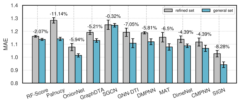
Figure 5. Performance improvements on PDBbind benchmark when training on general set.

In this section, we conduct experiments on two standard datasets to investigate the following research questions:

• RQ1. How does the proposed SIGN model perform compared against the state-of-the-art methods?

• RQ2. How does the generalizability of SIGN and competitors when trained on the larger but lower-quality dataset?

• RQ3. Do the spatial and interactive factors benefit the prediction?

• RQ4. How do the parameter settings (e.g., the cutoff distance and angle domain divisions) affect the prediction result?

5.1. Experiment Settings

5.1.1. Datasets.

We evaluate all models on the following public standard datasets for protein-ligand binding affinity prediction.

PDBbind is a well-known public dataset (Wang et al., 2005) in development which provides 3D binding structures of protein-ligand complexes with experimentally determined binding affinities (refer to Appendix A.2). In our experiment, we mainly use the PDBbind v2016 dataset, which is most frequently used in recent works (Stepniewska-Dziubinska et al., 2018; Zheng et al., 2019). Specifically, it includes three overlapping subsets, i.e., general, refined and core set. The general set contains all 13,283 protein-ligand complexes, while the 4,057 complexes in refined set are selected out of the general set with better quality. Moreover, the core set with 290 complexes serves as the highest quality benchmark for testing through a careful selection process (Su et al., 2018). Conveniently, we call the difference between the refined and core subsets, that is 3,767 complexes, as refined set of PDBbind in the following.

CSAR-HiQ is an additional benchmark dataset (Dunbar Jr et al., 2011), containing two subsets with 176 and 167 protein-ligand complexes. We use this external dataset from an independent source to further evaluate the generalization ability of models.

5.1.2. Setup.

Following (Ballester and Mitchell, 2010), we choose the refined set of PDBbind as our primary training data because there is considerable overlap between the full general set and CSAR-HiQ dataset. We randomly split the protein-ligand complexes in refined set with a ratio of 9:1 for training and validation. For testing sets, we use the core set and CSAR-HiQ set with removing the complexes present in refined set.

Since the lower-quality data of general set can still improve the performance of models (Li et al., 2015), we conduct the supplemental experiment on the full general set which is larger but of worse quality to analyze the generalizability of our model. As stated above, we can only evaluate the performance on the core set due to the overlapping problem of CSAR-HiQ dataset. Following (Stepniewska-Dziubinska et al., 2018; Zheng et al., 2019), we randomly select 1,000 complexes from refined set as the validating set. The remaining 11,993 complexes in general set are used for training.

5.1.3. Evaluation Metrics.

To comprehensively evaluate the model performance, following (Stepniewska-Dziubinska et al., 2018; Zheng et al., 2019), we use Root Mean Square Error (RMSE), Mean Absolute Error (MAE), Pearson’s correlation coefficient (R) and the standard deviation (SD) in regression to measure the prediction error. The detail is introduced in Appendix A.3.

5.1.4. Baselines.

We compare our proposed model with comparative methods including machine learning-based methods (LR, SVR, and RF-Score (Ballester and Mitchell, 2010)), CNN-based methods (Pafnucy (Stepniewska-Dziubinska et al., 2018) and OnionNet (Zheng et al., 2019)), and GNN models GraphDTA (Nguyen et al., 2020) for protein-ligand binding affinity prediction. Moreover, various state-of-the-art GNN-based models (SGCN (Danel et al., 2020), GNN-DTI (Lim et al., 2019), DMPNN (Yang et al., 2019), MAT (Maziarka et al., 2020), DimeNet (Klicpera et al., 2020), and CMPNN (Song et al., 2020)) which also consider the spatial information for molecular modeling are compared to evaluate the performance of SIGN. The details of experiment settings and baseline descriptions are provided in Appendix A.3 and A.4.

5.2. Performance Evaluation

5.2.1. Overall Comparison (RQ1).

We first compare our proposed SIGN with baseline approaches on two benchmark datasets. As shown in Table 2, the average and the standard deviation of four indicators for testing performance are reported across five random runs. In general, we can observe that SIGN achieves the best performance on two datasets, with 6.5% and 3.9% improvement of RMSE over the best baseline models on PDBbind and CSAR-HiQ datasets, respectively. We further have the following observations.

Among all baselines, GraphDTA methods show relatively poor performance due to the failure of considering the spatial structure and interactions between proteins and ligands. It indicates that simply modeling the molecular graph with protein sequence information is not capable of predicting structure-based protein-ligand binding affinity. By contrast, from the perspective of interaction modeling, the machine learning-based methods and OnionNet model take advantage of long-range interaction features and achieve better results. However, these data-driven approaches relying on feature engineering ignore the informative spatial structures of complexes and have limited generalization capability on the additional CSAR-HiQ dataset. From the perspective of spatial structural modeling, we find that SGCN and GNN-DTI which incorporate position and distance information exhibit considerable improvement over the vanilla GCN and GAT. Since SGCN takes atomic position coordinates as input directly, it will be easily affected by the rotation and translation of atoms, and the 3D CNN model Pafnucy suffers from a similar issue. Thus, the prediction results are not ideal. Despite leveraging a transformer-like attention mechanism to handle the spatial structure, MAT is not better than RF-Score and OnionNet, suggesting the importance of combining spatial and interactive information. The edge-oriented model CMPNN outperforms the above methods because it enhances DMPNN with communication while propagating the distance information, which shows the significance of node-edge message passing process. Although DimeNet can learn from angle information and perform slightly better, the performance is still not ideal due to its limited ability of modeling larger biomolecules. Our proposed SIGN can not only capture more comprehensive angle-enhanced structural information instead of just distance, but also handle interactions in the complex through multi-task learning framework. Therefore, SIGN is much effective for modeling the protein-ligand complex and can accurately predict the binding affinity.

5.2.2. Generalizability Comparison (RQ2).

There is increasing 3D structure-based protein-ligand data with binding affinity, whereas the amount of high-quality data in refined set is relatively small. Thus, the ability of utilizing more lower-quality data to improve performance shows the generalizability of model, which is another necessary measurement of performance evaluation. As introduced in Section 5.1.2, we conduct the extra experiment of generalizability on the general set of PDBbind dataset. As illustrated in Figure 5, we compare the proposed SIGN with major competitive baselines on two training sets. The results show that SIGN gets the lowest prediction error remarkably under both training settings. More importantly, our model improves the performance by around 8% when trained on the general set and it further expands the prediction advantage compared to baselines. Therefore, SIGN is proved to be more generalizable to more data in large quantity but poor quality.

5.2.3. Impact of Spatial and Interactive Factors (RQ3).

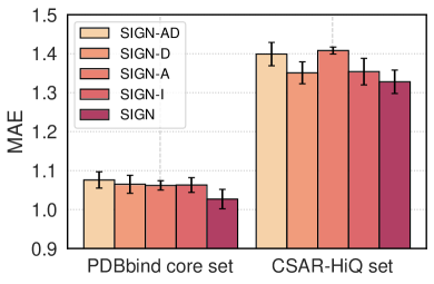
Figure 6. Contribution of spatial and interactive factors.

To verify the effectiveness of factors that influence the final performance, we compare SIGN with its variants on the two benchmarks.

• SIGN-AD uses the vanilla GAT layers for node-edge interaction without either angle or distance information.

• SIGN-D uses the vanilla GAT layer without distance information.

• SIGN-A uses the vanilla GAT layer without angle information.

• SIGN-I removes the interaction loss $\mathcal{L}_{z}$.

Figure 6 presents the comparison results on all metrics. As we can see, the proposed SIGN outperforms other variants, proving the necessity of handling the spatial and interactive information synergistically which is essential for protein-ligand binding affinity prediction. Specifically, SIGN-D and SIGN-A perform worse than SIGN since they can only capture the one-sided spatial structural information, i.e., distance or angle information in the complex. Furthermore, the prediction error of SIGN-AD is especially high among all variants. It indicates that modeling the complete spatial structure has a significant impact on performance improvement. The lack of long-range interactions in SIGN-I also leads to performance reduction, which confirms that only utilizing the spatial factors is insufficient and will lose the important interactive information.

5.2.4. Parameters Analysis (RQ4).

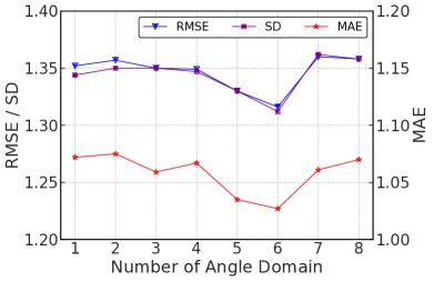
Figure 7. Parameter analysis on PDBbind core set.

As depicted in Figure 7, we investigate the performance variation for SIGN w.r.t several necessary hyper-parameters by varying each parameter while keeping others fixed as default settings. More results are in Appendix A.5.

Cutoff distance $\theta_{d}$. We analyze the effect of cutoff distance for complex graph construction when varying $\theta_{d}$ from 3 to 6. With the increase of $\theta_{d}$, more spatial information in the complex is available to our model and beneficial for learning complex representation better, which leads to dramatic performance improvements when $\theta_{d}\leq 5$ Å. After that, too long cutoff distance will introduce additional redundancies and degrade the performance.

Angle domain divisions $N$. To look deeper into the impact of angle information in our model, we divide the angle domains varying from 1 to 8. We can see that the model performs best when the number of angle domains is 5 or 6. Too fine-grained or coarse-grained divisions will result in performance degradation. One possible explanation is that too fine-grained divisions cannot provide distinguishable information in space while the angle domain at a too big granularity contains quite sparse atomic neighbors, both of which have an adverse effect on learning spatial information.

6. Conclusion

In this paper, we investigated how to improve the prediction of binding affinity between proteins and ligands. Specifically, we proposed a GNN-based model, SIGN, to learn the representations of protein-ligand complexes for better binding affinity prediction by leveraging the fine-grained structure and interaction information among atoms. Along this line, we designed the polar-inspired graph attention layers (PGAL) to integrate both distance and angle information for 3D spatial structure modeling. Also, to further improve the prediction performance, we introduced a well-designed pooling process along with a reconstruction learning task for interaction matrix. Finally, the experimental results on two benchmarks showed the effectiveness and the generalizability of the proposed model.

Appendix A Appendix

In the appendix, we first introduce the construction process of complex interaction graph. Then the details of experimental settings and baseline descriptions are given. Finally, we show the additional results of parameter analysis on another dataset. The pseudocode of SIGN training procedure is described in Algorithm 2. The implement our model based on PaddlePaddle. We train all models on 24 Intel CPUs and a Tesla V100 GPU with 32 GB memory. The code is available at: https://github.com/PaddlePaddle/PaddleHelix/tree/dev/apps/drug_target_interaction/sign.

A.1. Complex Interaction Graph Construction

As shown in Figure 2(a), there is no available intermolecular connection information between the ligand and its protein in the dataset. What’s more, the local covalent bonds in the original molecular graph cannot provide adequate 3D structure information. To include non-local correlations, here we aim to construct the spatial-based complex interaction graph. Since the size of a protein is much larger than that of a ligand, it’s unnecessary to build the complete protein structure in the complex graph, which might be noisy and time-consuming. Therefore, we apply a sampling-based process to construct the graph, which preserves the key structure of complex. The detail of the construction process is provided in algorithm 1. We first initialize the atom node set $\mathcal{V}$ with ligand’s atom set $\mathcal{V}^{L}$. Then the protein’s atoms which are close to the ligand from $\mathcal{V}^{P}$are selected to add into the atom node set $\mathcal{V}$. Finally, we update the complex edge set $\mathcal{E}$ by adding into the edges of atom pairs whose distances are smaller than the cutoff threshold $r_{\theta}$.

Input : The position matrix $M^{P}$  and node set $\mathcal{V}^{P}$of protein
The position matrix $M^{L}$  and node set $\mathcal{V}^{L}$  of ligand
The cutoff distance $r_{\theta}$

Output : The complex interaction graph $\mathcal{G}_{I}=<\mathcal{V},\mathcal{E}>$

1 Initialize $\mathcal{V}\leftarrow\mathcal{V}^{L}$, $\mathcal{E}\leftarrow\{\}$;

2 for atom node pair $(a_{i},\ a_{j})\in\mathcal{V}^{L}\times\mathcal{V}^{P}$ do

3       Calculate distance $d_{ij}\leftarrow|M^{L}(a_{i})-M^{P}(a_{j})|$;

4       if $d_{ij}\leq r_{\theta}$ then

5             Update node set $\mathcal{V}\leftarrow\mathcal{V}\cup\{a_{j}\}$;

6       end if

7      

8 end for

9Combined position matrix $M\leftarrow CONCAT(M^{L},M^{P})$;

10 for atom node pair $(a_{i},\ a_{j})\in\mathcal{V}\times\mathcal{V}$ do

11       Calculate distance $d_{ij}\leftarrow|M(a_{i})-M(a_{j})|$;

12       if $d_{ij}\leq r_{\theta}$ then

13             Update edge set $\mathcal{E}\leftarrow\mathcal{E}\cup\{e_{ij}=(a_{i},a_{j})\}$;

14       end if

15      

16 end for

return $\mathcal{V},\mathcal{E}$

Algorithm 1 Complex Interaction Graph Construction.

A.2. Instruction of the Binding Affinity

In biology experiments, the binding affinity between protein and ligand can be determined as the value $K_{d}$ (dissociation constant), $K_{i}$ (inhibition constant), or $IC_{50}$ (half inhibition concentration). In practice, the experimental binding affinity (i.e., the ground truth for the binding affinity prediction task) is expressed with the negative logarithm $pk_{a}$ of the determined value (e.g, $-logK_{d}$, $-logK_{i}$, or $-logIC_{50}$) on PDBbind and CSAR-HiQ datasets.

A.3. Experiment Details

A.3.1. Evaluation Metrics

We first detail the four metrics used in our experiment. Root Mean Square Error (RMSE), Mean Absolute Error (MAE) and Pearson correlation coefficient (R) are defined as:

(24) $$RMSE=\sqrt{\frac{1}{|\mathcal{D}|}\sum_{i=1}^{|\mathcal{D}|}(\hat{y}_{i}-y_{i})^{2}},\ MAE=\frac{1}{|\mathcal{D}|}\sum_{i=1}^{|\mathcal{D}|}|\hat{y}_{i}-y_{i}|$$

(25) $$R=\frac{\sum_{i=1}^{|\mathcal{D}|}(\hat{y}_{i}-\bar{\hat{y}})(y_{i}-\bar{y})}{\sqrt{\sum_{i=1}^{|\mathcal{D}|}(\hat{y}_{i}-\bar{\hat{y}})^{2}(y_{i}-\bar{y})^{2}}}$$

$\hat{y}_{i}$ and $y_{i}$ respectively represent the predicted and experimental binding affinity of the $i$-th complex in dataset $\mathcal{D}$. As introduced in (Stepniewska-Dziubinska et al., 2018), the standard deviation (SD) is defined as follows:

(26) $$SD=\sqrt{\frac{1}{|\mathcal{D}|-1}\sum_{i=1}^{|\mathcal{D}|}[y_{i}-(a+b\hat{y}_{i})]^{2}}$$

where $a$ and $b$ are the intercept and the slope of the regression line, respectively.

Input : Training set $\mathcal{D}$

Output : Trained model parameters $\theta$

1 Randomly initialize the parameter $\theta$ of SIGN;

2for iteration = 1, 2, … do

3       for each batch from training samples do

4             Calculate spatial relation embeddings $\bm{d}$ using Eq. (1);

5             for l = 1…L do

6                   Obtain edge embeddings $\bm{e}^{(l)}$ using Eq. (4)-(10);

7                   Obtain node embeddings $\bm{a}^{(l)}$ using Eq. (11)-(15);

8                  

9             end for

10            Build the interaction matrix $\bm{Z}$ using Eq. (16)-(17);

11             Estimate the interaction matrix $\tilde{\bm{Z}}$ using Eq. (18)-(19);

12             Calculate the interaction loss $\mathcal{L}_{z}$ using Eq. (20);

13             Calculate the prediction $\hat{y}$ using Eq. (21);

14             Calculate the prediction loss $\mathcal{L}_{a}$ using Eq. (22);

15             Update parameters $\theta$ according to the gradient of $\mathcal{L}$;

16            

17       end for

18      

19 end for

return $\theta$

Algorithm 2 Training Procedure for SIGN.

A.3.2. Input Graph and Features

For all GNN-based methods, we use the same input complex graph as introduced in Appendix A.1 for protein-ligand binding affinity prediction. For GraphDTA models, we input the protein sequence as well as the ligand molecular graph or our constructed complex graph. In this paper, we report the best result when using the complex graph as input. For 3D-CNN and GNN models, the atom features used according to (Stepniewska-Dziubinska et al., 2018) include atomic types, hybridization, the number of bonds with other heavy-atoms and hetero-atoms, atom properties such as aromaticity, and the partial charge. In total, 18 features are used to describe an atom. Considering the heterogeneity in the complex graph, we further extend atom features to a 36-dimension vector with zero-padding, where the 1st to 18th elements represent the features of ligand atoms and the 19th to 36th elements represent the features of protein atoms. As to edge features for edge-based GNN models, we combine the two atom features and encoded distance features between atoms as the input vector. In brief, we provide the same input complex graph and atomic features for our SIGN and all GNN-based baselines to make fair comparisons. For ML-based methods and OnionNet, they cannot take the complex graph or grid-like data as input and only receive the specific molecule-level features. We extract the input feature vectors based on the distance as described in their original papers (Ballester and Mitchell, 2010; Zheng et al., 2019). Note that these extracted features also reflect the structural information of complex in a global view.

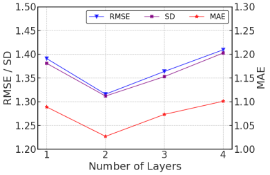
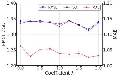
Figure 8. Parameter analysis on PDBbind core set.

A.3.3. Parameter Settings

For the proposed SIGN, we use Adam optimizer for model training with a learning rate of 0.001 and set the batch size as 32. The balancing hyper-parameter $\lambda$ is set to 1.75 according to the performance on validation set. We construct the complex graph and interaction matrix with cutoff-threshold $\theta_{d}=5Å$ and $\theta_{\rho}=12Å$ as suggested in (Muegge and Martin, 1999), respectively. The basic dimensions of node and edge embeddings are both set to 128. The number of buckets for spatial relation $b$ is set to 4 with the splitting granularity of 1Å. For PGAL layers, we set the number of attention heads $C$ to 4, the dropout rate to 0.2, and the number of angle domains $N$ to 6. For PiPool layer, there are 36 pooling blocks in total, where the two atomic type sets $S_{P}$ and $S_{L}$ are defined as stated in (Ballester and Mitchell, 2010).

For baseline models, we tune the parameters based on the default settings to get optimal performance. Specifically, the number of decision trees in RF-score is set to 100, the max-depth of trees is set to 5, the maximum number of features is set to 3 and the minimum number of samples required to split is set to 10. For the CNN-based models, we set the channels of three-layer 3D convolutions for Pafnucy as 64,128 and 256. For OnionNet, the number of input features is 3840 and there are 32, 64, and 128 filters in the three convolutional layers with the kernel size as 4. The maximum length of protein sequences is set to 1000 in GraphDTA. For GNN-based models, the number of filters in SGCN is set to 32 with the dimension as 36. We also apply the data augmentation process to ensure optimal performance. For fair comparison, the embedding dimension of other baselines is set to 128 (same as SIGN). For GNN-DTI, the initial $\mu$ and $\delta$ for distance learning in GAT layers are set to 4.0 and 1.0, respectively. For DimeNet, the number of spherical harmonics and radial basis functions are set to 4 and 3, respectively. We use two-layer interaction blocks and three-layer bilinear layers to make DimeNet work in our experiment. For DMPNN and CMPNN, the layer of edge-oriented message passing layers is set to 3 and we use MLP as the communication module in CMPNN. The weighting coefficients for self-attention, distance, and adjacency matrices in MAT are set to 0.3, 0.3, and 0.4, respectively.

A.4. Baseline Descriptions

We compare our SIGN model with the following methods to predict the protein-ligand binding affinity:

• ML-based methods include linear regression (LR), support vector regression (SVR), and random forest (RF). These methods take the inter-molecular interaction features introduced in RF-Score (Ballester and Mitchell, 2010) as input and predict the protein-ligand binding affinity.

• Pafnucy (Stepniewska-Dziubinska et al., 2018) is a representative 3D CNN-based model which can learn the spatial structure of protein-ligand complexes.

• OnionNet (Zheng et al., 2019) generates two-dimensional interaction features based on rotation-free element-pair contacts in complexes and adopts CNN to learn representations for prediction.

• GraphDTA (Nguyen et al., 2020) introduces GNN models to learn the complex graph and uses CNN to learn the protein sequence. It has four variants with different GNN models: GCN (Kipf and Welling, 2017), GAT (Veličković et al., 2018), GIN (Xu et al., 2019) and GAT-GCN which combines the former two models.

• SGCN (Danel et al., 2020) leverages node positions based on graph convolutional network, which directly utilizes atomic coordinates.

• GNN-DTI (Lim et al., 2019) is a distance-aware graph attention network with considering 3D structural information to learn the intermolecular interactions for protein-ligand complexes.

• DMPNN (Yang et al., 2019) is an edge-based message passing neural network. It can incorporate the spatial information between atoms by applying the aggregation process for edges.

• MAT (Maziarka et al., 2020) employs a molecule-augmented attention mechanism based on transformer for graph representation learning with using the inter-atomic distances.

• DimeNet (Klicpera et al., 2020) is a recent state-of-the-art model for small molecular graph learning using directional message passing scheme. Bessel functions are employed to encode the angle and distance information in graph neural network.

• CMPNN (Song et al., 2020) further develops DMPNN to build a communicative message passing scheme between nodes and edges for better molecular representation learning.

A.5. Additional Parameters Analysis

Number of PGAL layers $L$. As shown in Figure 8, we first present the influence of multi-hop propagation with stacking node-edge interaction layers from 1 to 4. We observe that increasing the number of layers would not always give rise to a better result. The model with one PGAL layer has limited ability to model high-order information in the complex. As a result of over-fitting, the performance of the model using more than 3 layers starts to degenerate gradually. Therefore, applying two interaction layers in SIGN is enough to capture sufficient spatial information.

Balancing coefficient $\lambda$. Moreover, we change the coefficient $\lambda$ to control the trade-off between the prediction loss and interaction loss. From the results, we observe that the performance first tends to get better with incorporating more interactive information for long-range dependencies, and then begins to drop off slightly. In general, our model is stable with varying coefficients and always achieves better performance than all baseline methods.

References

- (1)
- Allen et al. (2015) William J Allen, Trent E Balius, Sudipto Mukherjee, Scott R Brozell, Demetri T Moustakas, P Therese Lang, David A Case, Irwin D Kuntz, and Robert C Rizzo. 2015. DOCK 6: Impact of new features and current docking performance. Journal of computational chemistry 36, 15 (2015), 1132–1156.
- Ballester and Mitchell (2010) Pedro J Ballester and John BO Mitchell. 2010. A machine learning approach to predicting protein–ligand binding affinity with applications to molecular docking. Bioinformatics 26, 9 (2010), 1169–1175.
- Batool et al. (2019) Maria Batool, Bilal Ahmad, and Sangdun Choi. 2019. A structure-based drug discovery paradigm. International journal of molecular sciences 20, 11 (2019), 2783.
- Callaway (2020) Ewen Callaway. 2020. ’It will change everything’: DeepMind’s AI makes gigantic leap in solving protein structures. Nature (2020).
- Colwell (2018) Lucy J Colwell. 2018. Statistical and machine learning approaches to predicting protein–ligand interactions. Current opinion in structural biology 49 (2018), 123–128.
- Danel et al. (2020) Tomasz Danel, Przemysław Spurek, Jacek Tabor, Marek Śmieja, Łukasz Struski, Agnieszka Słowik, and Łukasz Maziarka. 2020. Spatial graph convolutional networks. In International Conference on Neural Information Processing. Springer, 668–675.
- Do et al. (2019) Kien Do, Truyen Tran, and Svetha Venkatesh. 2019. Graph transformation policy network for chemical reaction prediction. In SIGKDD. 750–760.
- Dunbar Jr et al. (2011) James B Dunbar Jr, Richard D Smith, Chao-Yie Yang, Peter Man-Un Ung, Katrina W Lexa, Nickolay A Khazanov, Jeanne A Stuckey, Shaomeng Wang, and Heather A Carlson. 2011. CSAR benchmark exercise of 2010: selection of the protein–ligand complexes. Journal of chemical information and modeling 51, 9 (2011), 2036–2046.
- Gohlke et al. (2000) Holger Gohlke, Manfred Hendlich, and Gerhard Klebe. 2000. Knowledge-based scoring function to predict protein-ligand interactions. Journal of molecular biology 295, 2 (2000), 337–356.
- Hao et al. (2020) Zhongkai Hao, Chengqiang Lu, Zhenya Huang, Hao Wang, Zheyuan Hu, Qi Liu, Enhong Chen, and Cheekong Lee. 2020. ASGN: An active semi-supervised graph neural network for molecular property prediction. In SIGKDD. 731–752.
- Jacob and Vert (2008) Laurent Jacob and Jean-Philippe Vert. 2008. Protein-ligand interaction prediction: an improved chemogenomics approach. Bioinformatics 24, 19 (2008), 2149–2156.
- Jain (2003) Ajay N Jain. 2003. Surflex: fully automatic flexible molecular docking using a molecular similarity-based search engine. Journal of medicinal chemistry 46, 4 (2003), 499–511.
- Jhoti and Leach (2007) Harren Jhoti and Andrew R Leach. 2007. Structure-based drug discovery. Vol. 1. Springer.
- Kinnings et al. (2011) Sarah L Kinnings, Nina Liu, Peter J Tonge, Richard M Jackson, Lei Xie, and Philip E Bourne. 2011. A machine learning-based method to improve docking scoring functions and its application to drug repurposing. Journal of chemical information and modeling 51, 2 (2011), 408–419.
- Kipf and Welling (2017) Thomas N. Kipf and Max Welling. 2017. Semi-Supervised Classification with Graph Convolutional Networks. In ICLR.
- Kitchen et al. (2004) Douglas B Kitchen, Hélène Decornez, John R Furr, and Jürgen Bajorath. 2004. Docking and scoring in virtual screening for drug discovery: methods and applications. Nature reviews Drug discovery 3, 11 (2004), 935–949.
- Klicpera et al. (2020) Johannes Klicpera, Janek Groß, and Stephan Günnemann. 2020. Directional Message Passing for Molecular Graphs. In ICLR.
- Leach et al. (2006) Andrew R Leach, Brian K Shoichet, and Catherine E Peishoff. 2006. Prediction of protein- ligand interactions. Docking and scoring: successes and gaps. Journal of medicinal chemistry 49, 20 (2006), 5851–5855.
- Leckband et al. (1992) DE Leckband, JN Israelachvili, FJ Schmitt, and W Knoll. 1992. Long-range attraction and molecular rearrangements in receptor-ligand interactions. Science 255, 5050 (1992), 1419–1421.
- Li et al. (2015) Hongjian Li, Kwong-Sak Leung, Man-Hon Wong, and Pedro J Ballester. 2015. Low-quality structural and interaction data improves binding affinity prediction via random forest. Molecules 20, 6 (2015), 10947–10962.
- Li and Shah (2017) Qingliang Li and Salim Shah. 2017. Structure-Based Virtual Screening. Methods in molecular biology (Clifton, N.J.) 1558 (2017), 111—124.
- Li et al. (2020) Shuangli Li, Jingbo Zhou, Tong Xu, Hao Liu, Xinjiang Lu, and Hui Xiong. 2020. Competitive Analysis for Points of Interest. In Proceedings of the 26th ACM SIGKDD International Conference on Knowledge Discovery & Data Mining. 1265–1274.
- Lim et al. (2019) Jaechang Lim, Seongok Ryu, Kyubyong Park, Yo Joong Choe, Jiyeon Ham, and Woo Youn Kim. 2019. Predicting drug–target interaction using a novel graph neural network with 3D structure-embedded graph representation. Journal of chemical information and modeling 59, 9 (2019), 3981–3988.
- Liu et al. (2021) Hao Liu, Jindong Han, Yanjie Fu, Jingbo Zhou, Xinjiang Lu, and Hui Xiong. 2021. Multi-Modal Transportation Recommendation with Unified Route Representation Learning. Proceedings of the VLDB Endowment 14, 3 (2021), 342–350.
- Liu et al. (2020) Yi Liu, Hao Yuan, Lei Cai, and Shuiwang Ji. 2020. Deep learning of high-order interactions for protein interface prediction. In SIGKDD. 679–687.
- Maziarka et al. (2020) Łukasz Maziarka, Tomasz Danel, Sławomir Mucha, Krzysztof Rataj, Jacek Tabor, and Stanisław Jastrz\kebski. 2020. Molecule Attention Transformer. arXiv preprint arXiv:2002.08264 (2020).
- Meng et al. (2011) Xuan-Yu Meng, Hong-Xing Zhang, Mihaly Mezei, and Meng Cui. 2011. Molecular docking: a powerful approach for structure-based drug discovery. Current computer-aided drug design 7, 2 (2011), 146–157.
- Moitessier et al. (2008) N Moitessier, P Englebienne, D Lee, J Lawandi, and CR Corbeil. 2008. Towards the development of universal, fast and highly accurate docking/scoring methods: a long way to go. British journal of pharmacology 153, S1 (2008), S7–S26.
- Muegge and Martin (1999) Ingo Muegge and Yvonne C Martin. 1999. A general and fast scoring function for protein- ligand interactions: a simplified potential approach. Journal of medicinal chemistry 42, 5 (1999), 791–804.
- Nguyen et al. (2020) Thin Nguyen, Hang Le, Thomas P Quinn, Tri Nguyen, Thuc Duy Le, and Svetha Venkatesh. 2020. GraphDTA: Predicting drug–target binding affinity with graph neural networks. Bioinformatics (10 2020). btaa921.
- Öztürk et al. (2018) Hakime Öztürk, Arzucan Özgür, and Elif Ozkirimli. 2018. DeepDTA: deep drug–target binding affinity prediction. Bioinformatics 34, 17 (2018), i821–i829.
- Ragoza et al. (2017) Matthew Ragoza, Joshua Hochuli, Elisa Idrobo, Jocelyn Sunseri, and David Ryan Koes. 2017. Protein–ligand scoring with convolutional neural networks. Journal of chemical information and modeling 57, 4 (2017), 942–957.
- Song et al. (2020) Ying Song, Shuangjia Zheng, Zhangming Niu, Zhang-Hua Fu, Yutong Lu, and Yuedong Yang. 2020. Communicative representation learning on attributed molecular graphs. In IJCAI. 2831–2838.
- Sousa et al. (2006) Sergio Filipe Sousa, Pedro Alexandrino Fernandes, and Maria Joao Ramos. 2006. Protein–ligand docking: current status and future challenges. Proteins: Structure, Function, and Bioinformatics 65, 1 (2006), 15–26.
- Stepniewska-Dziubinska et al. (2018) Marta M Stepniewska-Dziubinska, Piotr Zielenkiewicz, and Pawel Siedlecki. 2018. Development and evaluation of a deep learning model for protein–ligand binding affinity prediction. Bioinformatics 34, 21 (2018), 3666–3674.
- Su et al. (2018) Minyi Su, Qifan Yang, Yu Du, Guoqin Feng, Zhihai Liu, Yan Li, and Renxiao Wang. 2018. Comparative assessment of scoring functions: the CASF-2016 update. Journal of chemical information and modeling 59, 2 (2018), 895–913.
- Sun et al. (2020) Mengying Sun, Sendong Zhao, Coryandar Gilvary, Olivier Elemento, Jiayu Zhou, and Fei Wang. 2020. Graph convolutional networks for computational drug development and discovery. Briefings in bioinformatics 21, 3 (2020), 919–935.
- Trott and Olson (2010) Oleg Trott and Arthur J Olson. 2010. AutoDock Vina: improving the speed and accuracy of docking with a new scoring function, efficient optimization, and multithreading. Journal of computational chemistry 31, 2 (2010), 455–461.
- Veličković et al. (2018) Petar Veličković, Guillem Cucurull, Arantxa Casanova, Adriana Romero, Pietro Liò, and Yoshua Bengio. 2018. Graph Attention Networks. In ICLR.
- Wallach et al. (2015) Izhar Wallach, Michael Dzamba, and Abraham Heifets. 2015. AtomNet: a deep convolutional neural network for bioactivity prediction in structure-based drug discovery. arXiv preprint arXiv:1510.02855 (2015).
- Wang et al. (2005) Renxiao Wang, Xueliang Fang, Yipin Lu, Chao-Yie Yang, and Shaomeng Wang. 2005. The PDBbind database: methodologies and updates. Journal of medicinal chemistry 48, 12 (2005), 4111–4119.
- Wang et al. (2002) Renxiao Wang, Luhua Lai, and Shaomeng Wang. 2002. Further development and validation of empirical scoring functions for structure-based binding affinity prediction. Journal of computer-aided molecular design 16, 1 (2002), 11–26.
- Xu et al. (2019) Keyulu Xu, Weihua Hu, Jure Leskovec, and Stefanie Jegelka. 2019. How Powerful are Graph Neural Networks?. In ICLR.
- Yang et al. (2019) Kevin Yang, Kyle Swanson, Wengong Jin, Connor Coley, Philipp Eiden, Hua Gao, Angel Guzman-Perez, Timothy Hopper, Brian Kelley, Miriam Mathea, et al. 2019. Analyzing learned molecular representations for property prediction. Journal of chemical information and modeling 59, 8 (2019), 3370–3388.
- Zang and Wang (2020) Chengxi Zang and Fei Wang. 2020. MoFlow: an invertible flow model for generating molecular graphs. In SIGKDD. 617–626.
- Zheng et al. (2019) Liangzhen Zheng, Jingrong Fan, and Yuguang Mu. 2019. OnionNet: a Multiple-Layer Intermolecular-Contact-Based Convolutional Neural Network for Protein–Ligand Binding Affinity Prediction. ACS omega 4, 14 (2019), 15956–15965.
- Zheng et al. (2021) Zhi Zheng, Chao Wang, Tong Xu, Dazhong Shen, Penggang Qin, Baoxing Huai, Tongzhu Liu, and Enhong Chen. 2021. Drug Package Recommendation via Interaction-aware Graph Induction. arXiv preprint arXiv:2102.03577 (2021).
- Zhou et al. (2020) Jingbo Zhou, Shuangli Li, Liang Huang, Haoyi Xiong, Fan Wang, Tong Xu, Hui Xiong, and Dejing Dou. 2020. Distance-aware Molecule Graph Attention Network for Drug-Target Binding Affinity Prediction. arXiv preprint arXiv:2012.09624 (2020).