Robust Topology Optimization Using Variational Autoencoders

Abstract

Topology Optimization (TO) is the process of finding the optimal arrangement of materials within a design domain by minimizing a cost function, subject to some performance constraints. Robust topology optimization (RTO), as a class of TO problems, also incorporates the effect of input uncertainties, such as uncertainty in loading, boundary conditions, and material properties, and produces a design with the best average performance of the structure while reducing the response sensitivity to input uncertainties. It is computationally expensive to carry out RTO using finite element solvers due to the high dimensional nature of the design space which necessitates multiple iterations and the need to evaluate the probabilistic response using numerous samples. In this work, we use neural network surrogates to enable a faster solution approach via surrogate-based optimization. In particular, we build a Variational Autoencoder (VAE) to transform the the high dimensional design space into a low dimensional one, thus making the design space exploration more efficient. Furthermore, finite element solvers will be replaced by a neural network surrogate that predicts the probabilistic objective function. Also, to further facilitate the design exploration, we limit our search to a subspace, which consists of designs that are solutions to deterministic topology optimization problems under different realizations of input uncertainties. With these neural network approximations, a gradient-based optimization approach is formed to minimize the predicted objective function over the low dimensional design subspace. We demonstrate the effectiveness of the proposed approach on two compliance minimization problems: (1) the design of an L-bracket structure with uncertainty in loading angle, and (2) the design of a heat sink with varying load magnitude in the heat sources. Through these examples, we show that VAE performs well on learning the features of the design from minimal training data. Further, it also shows that converting the design space into a very low dimensional latent space makes the problem computationally efficient, and that the resulting gradient-based optimization algorithm produces optimal designs with lower robust compliances than those observed in the training set.

Keywords: Robust topology optimization, Variational Autoencoder, Deep neural networks, Shape parametrization.

1 INTRODUCTION

Topology Optimization is a rapidly expanding research area in various fields such as structural and industrial designs, mechanics, applied mathematics, and computer science [1]. Structural topology optimization seeks to determine the best distribution of a material within a prescribed design domain of a structure such that a cost function is minimized and certain performance constraints are satisfied. The pioneering numerical solutions to solve this problem was a homogenization approach proposed by Bendsoe and Kikuchi [4]. Since then, other solution approaches were developed including the density-based approach [5, 6, 7], level set approach [8, 9, 10], topological derivative method [11], phase field [12], and evolutionary approaches [13]. A widely used approach is the finite element based topology optimization method called SIMP (Solid Isotropic Material with Penalization for intermediate densities) [5, 14]. A detailed description of SIMP can be found in subsection 2.1.

The majority of works on structural topology optimization in the past two decades only consider deterministic performance. However, the performance of structures varies due to inherent uncertainties [3], mainly in loading [15, 16], boundary conditions [17], material properties [18, 20, 21] and geometry [22, 23]. In order to achieve robust and reliable designs, the effects of these uncertainties should be incorporated in the optimization process, giving rise to two types of topology optimization methods, namely Robust Topology Optimization (RTO) and Reliability Based Topology Optimization (RBTO). RTO methods attempt to maximize the deterministic performance of the structure while minimizing the sensitivity of the performance with respect to random parameters, resulting in a multi-objective optimization problem, capturing the impact of uncertainties in a qualitative sense. For an overview of robust optimization methods, the readers can refer to [18, 19]. On the other hand, in RBTO, introduced by Olhoff [24], reliability analysis is integrated into the element-based topology optimization method by adding a probabilistic constraint while keeping the objective function deterministic. Reliability-based topology optimization was further developed in recent years by various research groups [25, 26, 27]. An overview of RBTO methods can be found in [28, 29]. Some of the recent innovations in solving RBTO problems using deep learning and advanced sampling techniques can be found in [30, 31]. Topology optimization under uncertainties is still an open research area, with difficulties largely attributed to the high-dimensional property of design space which poses great challenges in uncertainty representation, propagation, and sensitivity analysis [18].

One of the major challenges of RTO is its computational expense attributed to the high dimensionality of design variables [32] and multiple iterations of optimizations [33]. This has led the researchers to study how data-driven machine learning algorithms can be used to address this issue. In design optimization, the application of deep learning has been explored in various problems [34], such as topology optimization [35, 36, 37, 38, 39], shape parametrization [40, 41], meta modeling [42, 43, 44], material design [45, 46, 47] and design preference [48].

Among the neural network models, convolutional neural network (CNN) models have been used for topology optimization with limited training data [49]. There has also been studies to predict the optimal designs under various input variables (e.g. loading magnitudes), where a feed forward neural network could be used to map the prescribed loading condition to the optimal design [50]. In order to improve the computational time, Yu [39] proposed a CNN-based encoder and decoder to generate a low resolution structure from a set of optimal topology designs. This low resolution structure is then upscaled using conditional Generative Adversarial Networks, thus avoiding Finite Element iterations. Guo [51] performed topology optimization on low dimensional latent space using variational autoencoder and style transfer. Cang [36] used active learning to improve the training of a neural network so that it would result in near optimal topologies.

Parametrization of design candidates using neural networks is another approach to achieve computational efficiency. It is an indirect design representation, where design variables are mapped to a typically low dimensional space, which could then be explored to find the best topology [51]. Since the parameterized mapping has lower dimension, it reduces the computational time significantly. In this approach, autoencoders has been used to parameterize the space of complex geometries [41]. However, autoencoders might produce infeasible geometries due to the gaps created in the latent space [52]. This could be addressed using variational autoencoders (VAE). Burnap [40] showed the possibility of parametrization of the 2D shape of an automobile using VAE. A detailed description of VAE and how it differs from autoencoders is given in subsection 2.4. It should be noted that the most of deep learning solution approaches for topology optimization were developed for deterministic problems and few studies have addressed robust topology optimization.

In this paper, we investigate how deep learning algorithms can facilitate the solution of robust topology optimization problems and shape parametrization. In particular, we focus on the compliance minimization problem, where the optimal design of the structure with loading uncertainty is identified. We have adopted a three stage approach to solve this problem. First, we parameterize the high dimensional geometry of the design candidates using a low dimensional representation obtained by VAEs. Secondly, we accelerate the cost (robust compliance) evaluation step in the optimization iterations by replacing the finite element solver with a fully connected deep neural network. Finally, we use gradient descent algorithm to find the optimal design on the low dimensional representation, minimizing the robust compliance. Training samples for both the neural networks are generated using SIMP or power law approach.

The remainder of this paper is organized as follows. A theoretical background on RTO and VAEs is presented in Section 2. Our proposed methodology for the robust topology optimization problem is then introduced in Section 3. Section 4 evaluates the performance of the proposed methodology when applied on a compliance minimization problem. Finally, Section 5 concludes the paper.

2 BACKGROUND

2.1 Deterministic Topology Optimization

Structural Topology Optimization can be defined as the arrangement of materials within a design domain to optimize the mechanical performance of the structure while accounting for design constraints [2]. In this paper, we restrict the discussion of the topology optimization problem to the well known compliance minimization design problem. The goal of this problem is to identify the topologies that store minimum strain energy under a set of applied loads, given a limited volume of material. Bendsoe [5], Zhou and Rozvany [7], and Mlejnek [6] proposed power-law or SIMP approach, where the design domain is discretized into elements called isotropic solid micro structures and the properties within these elements are assumed constant. According to Bendsoe [5], topology optimization involves determining, at an element level, whether there is material present or not. Thus, the density distribution of the material in the design domain, $\bm{\theta}$, is discretized into these elements, and the density of each element, $\theta_{\text{e}}$, is either 0 or 1 depending on whether material is present or not. However, in order to make the density distribution continuous, this density can vary from $\theta_{\text{min}}$ and 1, thus allowing intermediate densities for the elements. $\theta_{\text{min}}$ is the minimum allowable density for the elements ensuring the numerical stability of finite element analysis. For each element $e$, the density, $\theta_{\text{e}}$, and Young modulus of elasticity of the material, $E_{\text{0}}$, is related as $E(\theta_{\text{e}})=\theta_{e}^{p}E_{\text{0}}$, i.e. the power law. The penalty factor, $p$ assigns lower weight to the elements with intermediate densities, thus ensuring that the optimal topology moves towards solid black ($\theta_{\text{e}}=1$) or void white ($\theta_{\text{e}}=\theta_{\text{min}}$) design [53] .

Sigmund [54] provides a 99 line topology optimization code in MATLAB using the SIMP approach. Here, the design domain is considered to be rectangular and discretized by square finite elements with $n_{x}$ and $n_{y}$ being the number of elements in the horizontal and vertical directions. The topology optimization problem to minimize compliance using SIMP approach is written as

$$\underset{\bm{\theta}}{\text{minimize}} \mathrm{Q}(\bm{\theta})=U(\bm{\theta})^{T}K(\bm{\theta})U(\bm{\theta})$$ (1)

subject to $$\frac{V(\bm{\theta})}{V_{\text{0}}}=\alpha_{\text{v}}$$

$$K(\bm{\theta})U(\bm{\theta})=F_{\text{0}}$$

$$0<\bm{\theta}_{\text{min}}\leq\bm{\theta}\leq 1,$$

where $U$ and $F_{\text{0}}$ are the global displacement and force vectors, respectively, and $K$ is the global stiffness matrix. $\bm{\theta}_{\text{min}}$ is a vector of minimum densities, $V(\bm{\theta})$ and $V_{\text{0}}$ is the material volume and volume of the design domain, respectively, and $\alpha_{\text{v}}$ is the prescribed volume fraction with $0<\alpha_{\text{v}}\leq 1$.

The topology optimization problem described above is a deterministic one, as it aims to obtain the solution without taking into account the effects of uncertainties of input variables. The parameters or conditions that could be in general uncertain include the geometry, loading conditions, material properties, etc. In the next section, we present the formulation of a RTO problem which takes into account the impacts of these uncertainties.

2.2 Robust Topology Optimization

In RTO problems, a design is identified by minimizing a probabilistic form of the compliance. According to the original objective of RTO, we seek to solve a a two-objective optimization model which simultaneously minimizes the mean of the compliance and also its standard deviation. An efficient way to solve RTO is to combine the two objective functions into a single weighted function. For the sake of brevity, and in accordance with the examples in this paper, let us consider the RTO problem with uncertainty only in the loading. In particular, let $\bm{\theta}$ be the design variable and $\bm{\xi}$ be the random load. Then, the robust topology optimization formulation for minimizing the robust compliance, $Q_{\text{rob}}(\bm{\theta})$ can be written as [55]

$$\underset{\bm{\theta}}{\text{minimize}} \mathrm{Q}_{\text{rob}}(\bm{\theta})= \operatorname{\mathbb{E}}_{\bm{\xi}}\left[U(\bm{\theta},\bm{\xi})^{T}K(\bm{\theta})U(\bm{\theta},\bm{\xi})\right]+\lambda\ \left(\text{Var}_{\bm{\xi}}\left[U(\bm{\theta},\bm{\xi})^{T}K(\bm{\theta})U(\bm{\theta},\bm{\xi}))\right]\right)^{1/2}$$ (2)

subject to $$\frac{V(\bm{\theta})}{V_{\text{0}}}=\alpha_{\text{v}}$$

$$0<\bm{\theta}_{\text{min}}\leq\bm{\theta}\leq 1,$$

where $\operatorname{\mathbb{E}}_{\bm{\xi}}$ and $\text{Var}_{\bm{\xi}}$ are the expectation and variance operators with respect to the loading uncertainty $\bm{\xi}$. To calculate the compliance, the displacement for each realization of the random loading is calculated (predominantly using the finite element approach) by solving

$$K(\bm{\theta})\ U(\bm{\theta},\bm{\xi})=F_{\text{0}}(\bm{\xi}),\ \ \bm{\xi}\in S_{\bm{\xi}},$$

where $S_{\bm{\xi}}$ denotes the state space of random inputs. The constant $\lambda$ determines the balance between the mean and standard deviation; $\alpha_{\text{v}}$ is the prescribed volume fraction.

Robust topology optimization using finite element solvers are computationally expensive for high dimensional designs. In this study, we develop feed-forward fully-connected deep neural network surrogates to accelerate the response evaluations and VAEs to offer a low-dimensional representation for design variables $\bm{\theta}$.

2.3 Feed-forward fully-connected deep neural networks

Feed forward fully connected neural networks, or multi layer perceptrons (MLPs), are deep learning models which serve as a nonlinear mapping $\bm{y}=\mathcal{N}(\bm{x},\bm{\gamma})$, that approximates a target unknown function $\mathcal{N}^{*}(\bm{x})$. The model is built by learning the value of the neural network parameters, $\bm{\gamma}$, that results in the best function approximation. A fully connected neural network consists of a series of fully connected layers. A fully connected layer is a function from $\mathbb{R}^{\text{m}}$ to $\mathbb{R}^{\text{n}}$, and $\bm{x}\in\mathbb{R}^{\text{m}}$ represents the input and $\bm{y}\in\mathbb{R}^{\text{n}}$ is the $n$-dimensional model output. For instance, the output of a single hidden layer neural network, with $l$ nodes in the layer [56], can be calculated as

$$\mathbf{y}=\mathcal{A}(\mathbf{xW}_{\text{1}}+\mathbf{b_{\text{1}}})\mathbf{W_{\text{2}}}+\mathbf{b_{\text{2}}},$$ (3)

where $\mathcal{A}(.)$ is a non-linear function, known as the activation function, $\mathbf{W_{\text{1}}}$ and $\mathbf{W_{\text{2}}}$ are the weight matrices of size $m\times l$ and $l\times n$ and $\mathbf{b_{\text{1}}}$ and $\mathbf{b_{\text{2}}}$ are the bias vectors of size $1\times l$ and $1\times n$, respectively. A deep neural network has multiple hidden layers, where the output from the activation function from one hidden layer is transformed by new weight and bias values and fed to the next hidden layer [56]. A non-linear activation function enables the neural network to generate non-linear mappings from inputs to outputs. The most popular activation functions are sigmoid, tanh (Hyperbolic tangent) and ReLU (Rectified Linear Units). The ReLU activation function, one of the most widely used functions, has the form, $\mathcal{A}(x)=\max(0,x)$. Sigmoid function has the form, $\mathcal{A}(x)={1}/({1+\exp(-x)})$, and ranges between 0 and 1. The neural network architectures in the present study use ReLU to activate the hidden layers. The output layer of the Variational Autoencoder is activated by sigmoid function to ensure that the density values range between 0 and 1.

2.4 Variational Autoencoders

An autoencoder is a neural network model that learns a compact representation of a data (e.g. an image or a vector), while retaining its most important features. It consists of a pair of connected neural networks - an encoder and a decoder. The encoder network takes an input from a typically high-dimensional space and converts it into a lower dimensional representation known as the latent space. The decoder network takes a point from the latent space and reconstructs a corresponding output in the original space. The encoder and decoder neural networks are trained together and optimized via back-propagation[57]. In the context of structural topology, the training set includes $n$ topologies, $[\bm{\theta}_{1},\bm{\theta}_{2},\bm{\theta}_{3},...,\bm{\theta}_{n}]$. Using these samples, the training of the autoencoder is carried out by minimizing the reconstruction error [52],

$$L_{\text{reco}}=\displaystyle\sum_{i=1}^{n}\|\bm{\theta}_{i}-\hat{\bm{\theta}}_{i}\|^{2},$$ (4)

where $\bm{\theta}_{i}$ is the $i$-th topology sample and ${\hat{\bm{\theta}}}_{i}$ is its corresponding reconstructed topology, respectively. The hidden layers could be convolutional, fully connected or could take any other form depending on the task at hand. In this work, we have used fully connected deep neural networks for the encoder and decoder networks.

The fundamental problem with autoencoders is that the trained latent space may not be continuous, or may not allow easy interpolation[58]. If the latent space has discontinuities (e.g. gaps between clusters) and the topology that is generated by a sample from one of the gaps may be an unrealistic geometry. This is because, the autoencoder, during training, has never seen encoded vectors from that region of latent space. This challenge could be addressed by the use of Variational Autoencoder (VAE).

A VAE, like an autoencoder, consists of an encoder, a decoder and a loss function. The encoder neural network, denoted by $f(\cdot)$, encodes an input topology, $\bm{\theta}$, to a (random) latent variable $\bm{z}$, i.e. $\bm{z}=f(\bm{\theta})\sim q(\bm{z}|\bm{\theta})$. The decoder network of VAE, denoted by $g(\cdot)$, decodes a given (random) latent variable, $\bm{z}$, back to an image similar to the original input, i.e. $\bm{\hat{\theta}}=g(\bm{z})\sim p(\bm{\theta}|\bm{z})$. Here, $\bm{\hat{\theta}}$ is the vector of reconstructed images by the decoder network, generated from the latent vector, $\bm{z}$. Let the latent representation, $\bm{z}$, be sampled from the prior distribution, $p(\bm{z})$. The latent space is regularized for the purpose of continuity (two close points in latent space gives similar output) and completeness (the generated output should not be non-meaningful). To satisfy this, it is required to regularize both the covariance matrix and the mean of the latent space distribution[59]. This is done by enforcing the prior distribution to be a standard normal distribution, i.e., $p(\bm{z})\sim\mathcal{N}(0,1)$.

The loss function of VAE consists of a reconstruction loss term and a regularizer. Let $[\bm{\theta}_{1},\bm{\theta}_{2},\bm{\theta}_{3},...,\bm{\theta}_{n}]$, be the set of topology samples, then the total VAE loss is given by

$$L_{\text{VAE}}=\sum_{i=1}^{n}l_{i}$$ (5)

where $l_{i}$ is the loss function for the $i$th data point (sampled topology), given by

$$l_{i} =-\operatorname{\mathbb{E}}_{\bm{z}\sim q(\bm{z}\mid\bm{\theta}_{i})}[\log(p(\bm{\theta_{i}}\mid\bm{z}))]+\text{KL}(q(\bm{z}\mid\bm{\theta}_{i})\mid\mid p(\bm{z})).$$ (6)

The first term is the reconstruction loss, or expected negative log-likelihood of the $i$th data point. It measures how likely it is that the data point $\bm{\theta}_{i}$ is explained by the random variable $\bm{z}$. The prior distribution for the VAE latent variables, $p(\bm{z})$, is taken to be a standard normal distribution. The expectation in Equation 6 is taken with respect to $q(\bm{z}\mid\bm{\theta}_{i})$, which is referred to as the ‘encoder distribution’. In calculating the likelihood, we use this distribution instead of the prior $p(\bm{z})$ (which doesn’t depend on $\bm{\theta}$) in order to promote sampling from $\bm{z}$ values that are expected to have contribution to the training data. Otherwise, one may obtain many samples from the latent space for which the training data is improbable, i.e. $p(\bm{\theta}\mid\bm{z})=0$.

Since we use encoder distribution instead of the prior $p(\bm{z})$, in the derivation of the loss function, we will also obtain the second term in the left hand side of Equation 6, which serves as a regularizer. This term is the Kullback-Leibler (KL) divergence between the encoder distribution $q(\bm{z}\mid\bm{\theta})$ and the prior $p(\bm{z})$ and measures how much information is lost when distribution $q$ is instead of $p$. A detailed derivation of the loss function of VAE can be found in [59, 60].

During the training of VAE, the decoder randomly samples the latent vector, $\mathbf{z}$, from the encoder distribution, $\mathbf{z}\sim q(\mathbf{z})$. But, the back propagation cannot flow through random sampling and hence, a reparametrization technique is used, where $\mathbf{z}$ is approximated by the following normal distribution [52],

$$\bm{z}\sim\mathcal{N}(\bm{\mu},\text{diag}(\bm{\sigma}))$$ (7)

where $\bm{\mu}$ and $\bm{\sigma}$ are set to be the output vectors from the encoder network, $f$. An overview of the VAE neural network architecture is shown in Figure 1.

In the present study, the encoder network consists of input layer, which is the vectorized version of the input topology images, a number of fully connected hidden layers and the latent space layer as the output layer. The number of nodes in the latent space layer depends on the latent space dimension, $|\bm{z}|$. There are two outputs from the encoder network - vectors of $\bm{\mu}$ and $\bm{\sigma}$ values, which are the input to the decoder network. The decoder network, like the encoder, consists of an input layer, with size $|\bm{z}|$, and the output layer which gives the reconstructed/generated topology, and thus has the same number of nodes as the input layer of the encoder network. In this work, we use a train VAE as a means to map high dimensional topology data into a low dimensional space, and also map new samples in the latent space into newly generated topologies.

Figure 1: An overview of the neural network structure of a VAE with a two dimensional latent space. It consists of an encoder network and decoder network. The input of the encoder network is the image of a topology and the output of the decoder network is the corresponding reconstructed topology. The encoder maps the high dimensional input data to a low dimensional vector, $[z_{1},z_{2}]$, which becomes the input to the decoder network.

3 METHODOLOGY

Using the formulation in Eq. 2, the objective of the study is to find the optimal design variable, $\bm{\theta}^{*}$, which minimizes $Q_{\text{rob}}(\bm{\theta})$. We do so by solving the optimization problem minimizing a sample-based approximation of the robust compliance given by

$$\underset{\bm{\theta}}{\text{minimize}} \mathrm{Q}_{\text{rob}}(\bm{\theta})\approx \frac{1}{n}\sum_{i=1}^{n}Q_{i}(\bm{\theta})+\lambda\left({\frac{1}{n}\sum_{i=1}^{n}(Q_{i}(\bm{\theta})-\mu_{\text{Q}})^{2}}\right)^{1/2}$$ (8)

subject to $$\frac{V(\bm{\theta})}{V_{\text{0}}}=\alpha_{\text{v}}$$

$$0<\bm{\theta}_{\text{min}}\leq\bm{\theta}\leq 1,$$

where $Q_{i}(\bm{\theta})=U(\bm{\theta},\bm{\xi}_{i})^{T}K(\bm{\theta})U(\bm{\theta},\bm{\xi}_{i})$, is the deterministic compliance, calculated based on the global stiffness matrix $K(\bm{\theta})$ and the global displacement vectors for the $i^{\text{th}}$ realization of the random input parameter; and $\mu_{\text{Q}}:=\frac{1}{n}\sum_{i=1}^{n}Q_{i}(\bm{\theta})$.

The search space for the solution of this optimization problem is the set of all the designs $\bm{\theta}$, each evaluated at all the realizations of the random parameter, $\bm{\xi}$. Because of the high dimensional representation of topologies, it is computationally challenging to carry out optimization in this search space. As a remedy, we consider a subspace of the search space, which consists of only the deterministic designs that are optimal with respect to particular realizations of $\bm{\xi}$. To create this space, we undertake a supervised learning approach, and obtain these deterministic designs from the SIMP algorithm given various realizations of input. This search subspace ensures that we have a relatively good initial space of candidate designs, without having to run any RTO solver.

In particular, our RTO solution approach, shown in Figure 2, consists of three stages. The first stage is the parameterization of our search subspace to reduce the dimensionality of the design representations. There are a variety of approaches for doing this, a review of which could be found in [61]. In the present study, VAEs are used to represent the geometries in terms of latent space distribution, which could be then used to reconstruct the original designs. One of the main advantages of using VAE is the reduction in dimensionality, from thousands to as low as 2. The second stage is the fast estimation of the robust compliance for candidate designs using a feed forward fully connected compliance neural network surrogate. The final stage is finding the optimal design which minimizes the robust compliance using a gradient-based optimization process, which involves backpropagation through the compliance network and the decoder part of the VAE, as shown in Figure 2. In what follows, we provide details about these networks.

Figure 2: The complete neural network architecture for topology optimization. The top image shows the training of the VAE network and the compliance neural network surrogate. The bottom image shows how gradient descent is applied for finding the optimal design for the compliance minimization problem.

3.1 Neural Networks for Dimensionality Reduction and Robust Compliance Prediction

As illustrated in Figure 2, the first part of the solution approach is the dimensionality reduction of the designs using VAE. These designs are the input, $\bm{\theta}$, to the encoder network of VAE, $f(\cdot)$. The images used for training VAE are a sample of geometries from the search subspace, which are the deterministic optima obtained at various realizations of $\bm{\xi}$. The encoder network consists of an input layer, a number of fully connected hidden layers and an output layer, which are the mean and standard deviation values for the latent variable $\bm{z}$. ReLU function is used as the activation function for all the hidden layers. The decoder network, $D$, consists of an input layer, a number of fully connected hidden layers, an AVG (average) pooling layer and an output layer. The input layer has $|\bm{z}|$ number of nodes. ReLU function is used as the activation function for all the hidden layers.

The output of the last hidden layer, which has the same dimension as the input image,$\bm{\theta}$, is passed through an AVG pooling layer. The pooling layer acts as a design filter, to ensure that the reconstructed image does not have checker board pattern. It does this by replacing the pixel value with the average of its neighboring pixel values. The output of the AVG pooling layer is, then, passed through a sigmoid function to make sure all the pixel values are between 0 and 1 to get the final reconstructed image. Finally, the entire VAE network is trained by updating its weights and biases to reduce the loss function of Equation (6).

The second part of the solution is to have a computationally efficient method to calculate the robust compliance of the candidate designs, $Q_{\text{rob}}(\bm{\theta})$. This is done by training a compliance neural network surrogate, which is a feed forward fully connected deep neural network, consisting of an input layer, a number hidden layers and an output layer. Input layer has number of nodes equal to the dimension of the training image. Output layer is a single node which gives predicted robust compliance, $Q_{\text{NN}}(\bm{\theta})$. The loss function for the training of the network is the mean squared error between $Q_{\text{rob}}(\bm{\theta})$ and the output of the neural network, $Q_{\text{NN}}(\bm{\theta})$. ReLU function is used as the activation function for all the layers and Adam optimizer is used for the training of the neural network with a constant learning rate.

3.2 Gradient-based RTO via Low Dimensional Space

The final stage of the solution is to find the optimal design from the generated designs from VAE. One of the fundamental methods is the brute force method, where we generate various designs from the search space, compute $Q_{\text{NN}}$ using compliance neural network surrogate and find the design with the minimum compliance. However, this is not an efficient approach and would not guarantee that the design is the most optimal one. Therefore, we use a gradient-descent algorithm for finding the most optimal design for the topology optimization problem.

Using stochastic gradient descent on on the compliance surrogate, one can optimize the topology according to the robust compliance criterion. Specifically, at step $i+1$ of the gradient descent, we can use the following update rule

$${\bm{\theta}}_{\text{i+1}}={\bm{\theta}}_{\text{i}}-\eta\nabla{Q_{\text{NN}}}(\bm{\theta}_{\text{i}}),$$

where ${\bm{\theta}}_{\text{i}}$ and ${\bm{\theta}}_{\text{i+1}}$ are the designs at steps $i$ and $i+1$ of the gradient descent journey, and $\nabla{Q_{\text{NN}}}(\bm{\theta}_{\text{i}})$ is the gradient of the compliance calculated on the $i$th geometry.

This update rule is not efficient, however, as the topology $\bm{\theta}$ is typically high dimensional and this can significantly slow down the algorithm. To improve the computational speed and reduce the dimensionality of the input, we instead consider the lower network in Figure 2, which consists of the decoder part of the VAE and the compliance surrogate. Using this network, we compute the gradient of the robust compliance with respect to the latent space encoding of the geometry, i.e. $\bm{z}$. Therefore, the gradient descent update can be rewritten as

$${\bm{z}}_{\text{i+1}}={\bm{z}}_{\text{i}}-\eta\nabla{Q_{\text{NN}}}(\bm{z}_{\text{i}}),$$

and the dimension of the gradient calculation is reduced to $|\bm{z}|$. Using this update rule, we effectively search the lower dimensional latent space for the optimal $\bm{z}$. The gradient descent updates begin on a randomly selected initial point in the latent space. It is imperative to try multiple starting points to ensure that the algorithm does not converge to a local minima with a poor compliance.

So we effectively identify the robust design by solving the following unconstrained optimization

$$\underset{\bm{z}}{\text{minimize}}\ \ \mathrm{Q}_{\text{NN}}(\bm{z})=h\circ g\ (\bm{z}),$$ (9)

where $g(\cdot)$ is the decoder part of the VAE which serves as the generator of candidate designs, and $h(\cdot)$ is the approximate predictive model for robust compliance.

4 RESULTS

In this section, we demonstrate the effectiveness of our proposed methodology in solving the robust topology optimization in two problems - an L-shaped bracket with uncertainty in load angle, and a heat conduction problem with a heat sink with a fixed location but uncertain load magnitude.

4.1 L-bracket with loading uncertainty

As the first example, we consider an L-shaped structure with fixed boundary and a single point load. The applied load has a fixed magnitude but a known random angle. An example of a candidate topology is shown in Figure 3. The load angle is calculated as the angle from the downward vertical line in the counter clockwise direction and is considered to be uniformly distributed between 0 and $\pi$. In this example, the resolution of the images representing the topology is considered to be $100\times 100$, and therefore the input $\bm{\theta}$, defining the geometry of the structure, is a $n_{\bm{\theta}}=10,000$ dimensional vector. The random input $\bm{\xi}$ in this case is a single random variable (i.e. $n_{\xi}=1$), namely the load angle. The objective is to find the optimal design, $\bm{\theta}^{*}$, via finding the optimal $\bm{z}^{*}$, which minimizes the robust compliance of the structure, $Q_{\text{rob}}$, given the uncertain load angle.

Figure 3: An example of the structure used in our study. The top part of the L-shaped structure has a fixed boundary. The load is applied at a single point with uncertainty in loading angle, $\bm{\xi}$, calculated as the angle from downward vertical line in the counter clockwise direction.

4.1.1 Evaluation of the VAE reconstruction and generation

In the first step, in order to build the search subspace using VAE, we need to obtain the training data, which are deterministic optimal designs at various realizations of load angle calculated using the SIMP approach. In particular, we considered 1000 load angle samples between $0$ and $\pi$ and obtained the corresponding deterministic designs using the 88 line topology optimization code in Matlab [62]).

As a result, this data set includes 1000 topology samples, with each data point consisting of 100 $\times$ 100 pixels. Next, we need to train a VAE to encode these 10,000 dimensional topology data into a latent space with a much smaller dimensionality. In this work, we removed the 10 top-ranked topologies based on their compliances, i.e. the 10 geometries that yielded the 10 lowest robust compliance values. This was done in order to study whether the resulting search subspace is capable of encoding topologies that are better performing than those seen in the training set. Out of the rest 990 geometries, we used 90 images for testing and $n_{train}$ images for training, with $n_{\text{train}}=100,200,\cdots,900$ as will be explained later. Also, we considered various latent space dimensions, specifically $|\bm{z}|=2,5,10$, in order to study how the dimensionality of the latent space would impact the performance of the representation and the subsequent optimization process.

The training images are the input to the encoder network, which consists of an input layer, 7 fully connected hidden layers and an output layer. The output layer is the latent space layer. The number of nodes in the seven hidden layers are 5000, 2500, 1000, 500, 100, 50 and 10 respectively. Input layer has 10,000 nodes, same as the number of features from the input image (100$\times$ 100 pixels). The number of nodes in the latent space layer depends on the chosen latent space dimension, $|\bm{z}|$. ReLU function is used as the activation function for all the hidden layers.

The decoder network consists of an input layer, eight fully connected hidden layers, an AVG (average) pooling layer and an output layer. The input layer has $|\bm{z}|$ number of nodes. The eight hidden layers in the decoder network has number of nodes 10, 50, 100, 500, 1000, 2500, 5000 and 10000 respectively. ReLU function is used as the activation function for all the hidden layers. The output of the eighth hidden layer, which has the same dimension as the input image, is passed through an AVG pooling layer with $9\times 9$ window. The AVG pooling layer ensures that the output image does not have checkerboard pattern.

Figure 4 shows how different choice of $n_{\text{train}}$ impact the testing loss of VAE, for $|\bm{z}|=2$. We can observe that with $n_{\text{train}}=400,600$, the error converges more quickly compared to the case with $n_{\text{train}}=200$. However, their loss values do not vary much. In order to study the impact of latent space dimension, $|\bm{z}|$, on the performance of VAE representation, we trained the model for $|\bm{z}|=2,5,10$. Figure 5 shows how the testing loss of VAE for different values of $|\bm{z}|$, when training is done with $n_{\text{train}}=600$. It can be observed that $|\bm{z}|$ does not have a noticeable impact on the convergence of the training.

Figure 4: Total testing loss for various training sample sizes, $n_{\text{train}}$. Total loss is the sum of reconstruction error and KL Divergence. The results are shown for $|\bm{z}|=2$.

Figure 5: Total testing loss for various latent space dimensions, $|\bm{z}|$. Total loss used is the sum of reconstruction error and KL Divergence. The results are shown for $n_{\text{train}}=600$.

As samples for the results, Figure 6 shows four test images and their corresponding reconstructed images from VAE. As evident from the figure, the VAE reconstructs the original image with high accuracy. We can also generate new images, not present in the training or testing data set, by sampling from the prior distribution of $\bm{z}$, and feeding it to the decoder network. Figure 7 shows a sample of 16 images generated by sampling $\bm{z}$ from $N(0,\bm{I})$ for VAE with $n_{\text{train}}=600$. We can observe that the generated images are of good quality, closely resembling the overall structure of the training images, but with variation in the detailing of the design. A notable observation is that, even without imposing the volume fraction constraint of the optimization problem through the loss function, the network is able to learn this feature through training and is able to impose it on its output. In our experiments, only less than 1% of the generated images from VAE has volume fraction, $\alpha_{\text{v}}>0.4$, with maximum volume fraction less than 0.405.

(a) Images from the testing dataset

(b) Reconstructed images from NN_{unconstrained}

Figure 6: Comparison between the test images (top) with their corresponding reconstructed images from VAE (bottom).

Figure 7: A representative collection of topologies generated by the decoder network of the VAE, via sampling from the standard normal $\bm{z}$ with $|\bm{z}|=2$ and $n_{\text{train}}=600$ using VAE.

4.1.2 Evaluation of the compliance neural network surrogate

The compliance neural network surrogate, $h(\cdot)$, is a fully connected deep neural network with one input layer, seven hidden layers and an output layer. Input layer has 10,000 nodes (equal to the dimension of the topology images $\bm{\theta}$). The hidden layers have 5000, 2500, 1000, 500, 100, 50 and 10 nodes, respectively. Output layer is a single node which predicts the robust compliance value, $Q_{\text{NN}}$. Adam optimizer is used to minimize this loss function, with a constant learning rate of 1e-4. The compliance neural network is trained using the 1000 images generated using SIMP. The robust compliance values of the topologies are calculated using the quadrature method. A total of seven quadrature points, sampled between 0 and 1 and scaled to be in the range of the load angle, and corresponding quadrature weights are used for calculating the robust compliance. For each topology, the deterministic compliance values, $Q$, are calculated for load angles corresponding to each of the quadrature points and they are averaged using the corresponding quadrature weights to calculate the robust compliance, $Q_{\text{rob}}$. Figure 8 shows the accurate prediction of the compliance surrogate after only 100 training iterations.

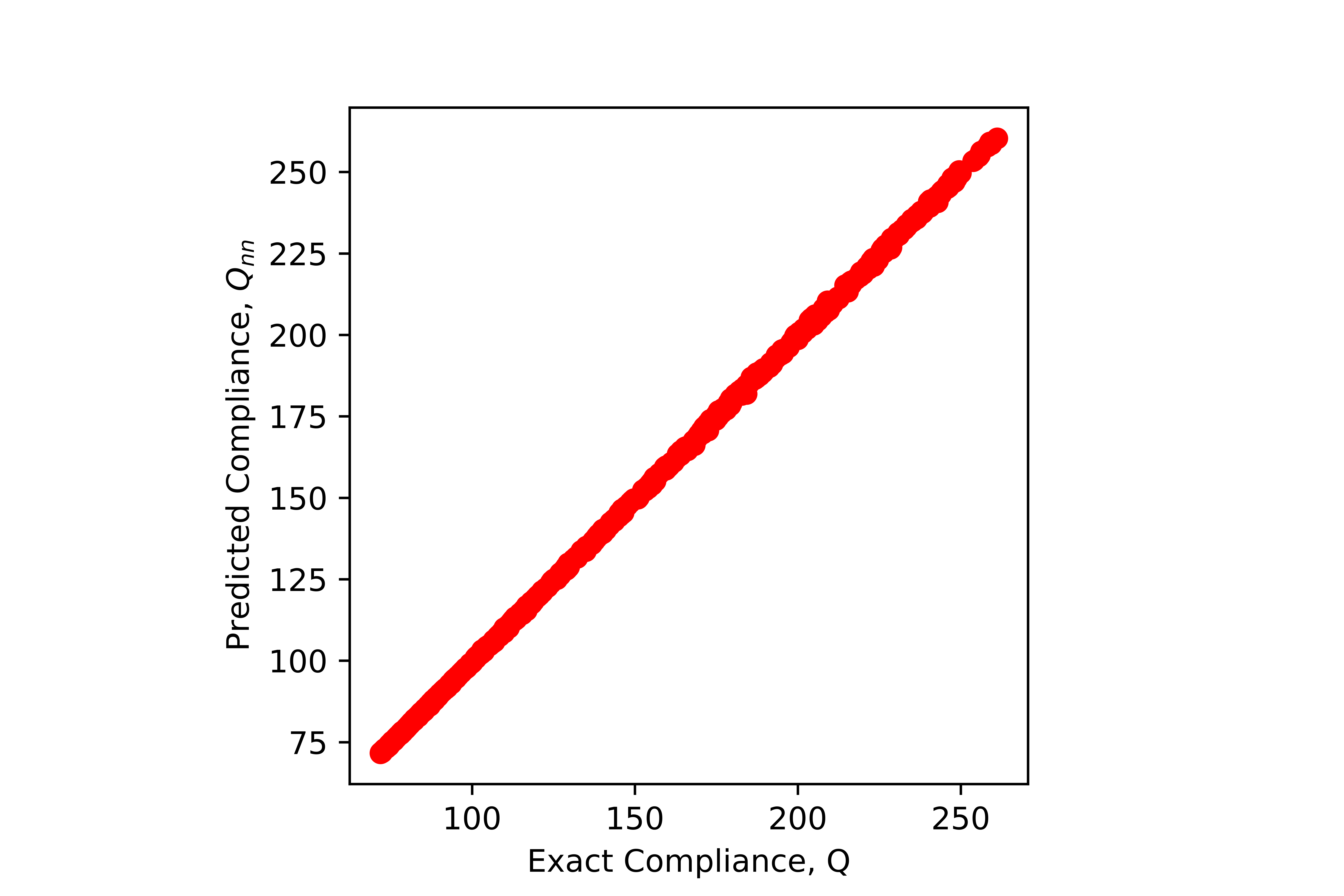
Figure 8: The comparison between the “exact” values of robust compliance, $Q_{rob}$, with the predicted robust compliance $Q_{\text{NN}}$. The training converged after 100 iterations where the loss function is the mean squared error between the “exact” robust compliance calculated using quadrature method and the predicted one.

4.1.3 Evaluation of the gradient descent optimization

Using the trained VAE and compliance surrogates, we solve the RTO problem by solving the unconstrained problem in Equation 9. This involves applying gradient descent algorithm in the latent space (as shown in Figure 2). One of the shortfalls of gradient descent is the possibility of designs to optimize to local minima instead of global minima. Figure 10 shows how starting at different $\bm{z}$ values can lead to different local minima. In order to avoid this and to start with a good initial design $\bm{z}_{0}$ , we use a brute-force approach where we draw a moderate number of $\bm{z}$ samples and evaluate their approximate robust compliance, $Q_{\text{NN}}$, and select the design with the lowest compliance as the initial point for the gradient descent step.

Figure 9 shows the optimal designs obtained through this process where 100 initial samples were used to determine the best initial design. Out of the 1000 deterministic designs obtained from SIMP, the best one had a robust compliance of $Q_{\text{rob}}=71.59$. As mentioned earlier, the top ten deterministic designs (based on the robust compliance value) are not included in the training of the VAE. Here, we have included the results of two VAEs trained with $n_{\text{train}}=200$ and $n_{\text{train}}=600$. Both the models had latent space dimension of $|\bm{z}|=2$, which showed the same performance levels compared to higher dimensions. The VAE with $n_{\text{train}}=200$ is computationally much faster to train and the resulting gradient descent produces a design that is better than the training samples. The VAE with $n_{\text{train}}=600$ produced the best design via the gradient descent approach, with $Q_{\text{rob}}=69.84$ which was smaller than $Q_{\text{rob}}=71.89$ observed in the training data. This design is better, in terms of the robust compliance, than the best design from the deterministic optimal space as well. Figure 10 shows the evolution of the gradient descent from the starting image to its optimal design. These results underscore the effectiveness of the approach to efficiently explore the search subspace and its capability to improve the design beyond the training set. It should however be noted that it cannot still outperform the best robust design obtained from SIMP mainly because a smaller subspace is being explored.

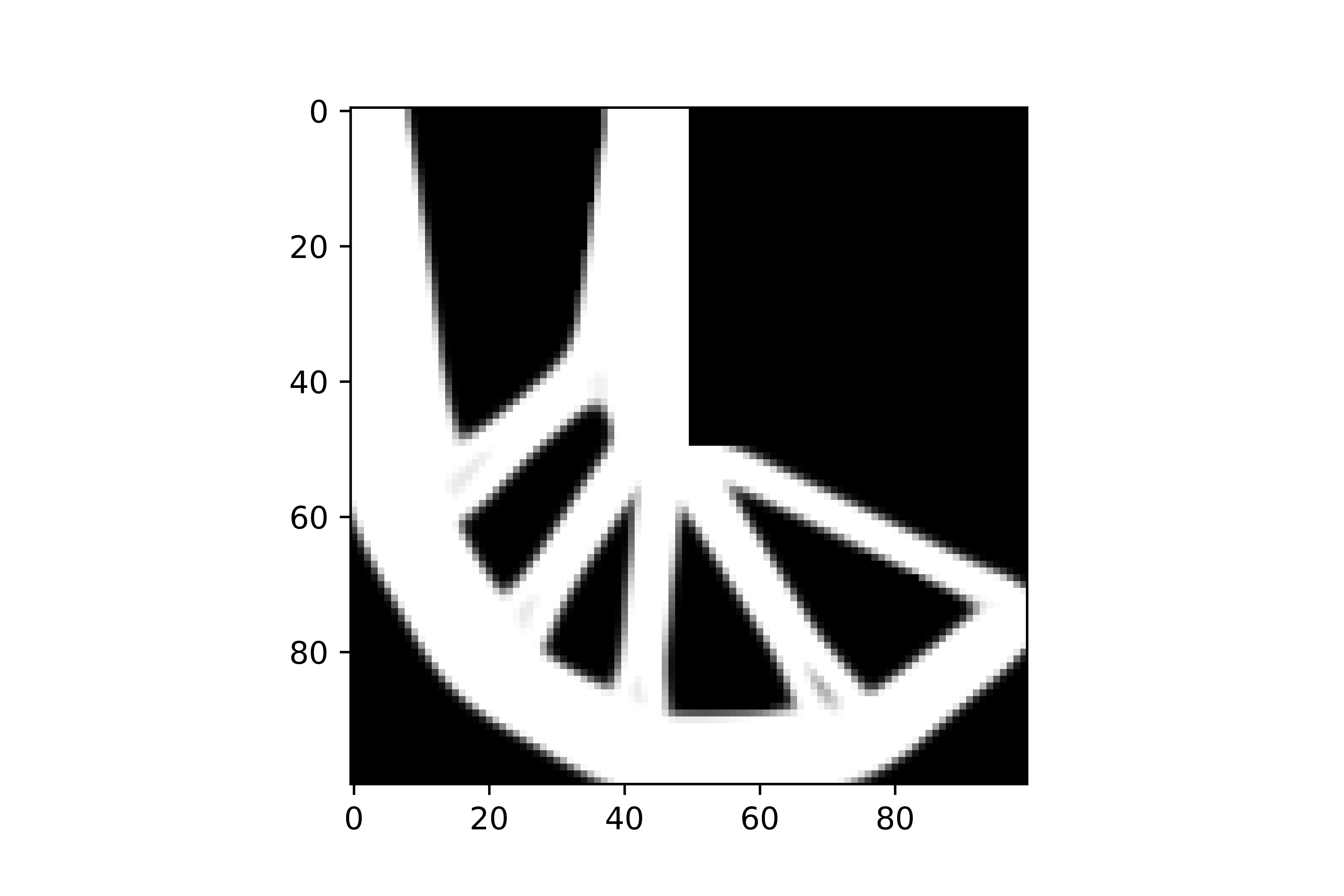
(a) Best design from the deterministic optima space, $Q_{\text{rob}}=71.59$

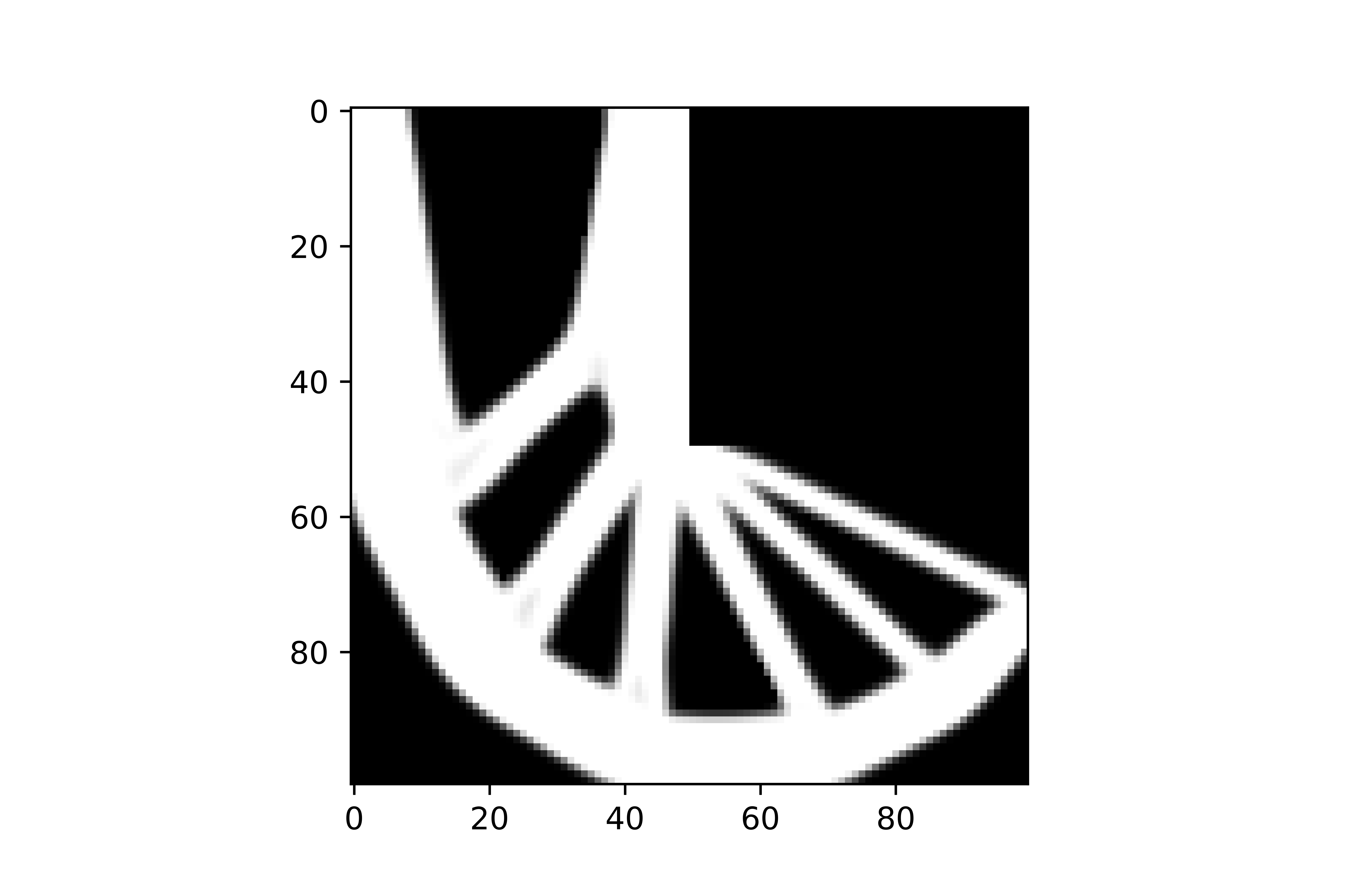
(b) Best design in the training data for $n_{\text{train}}=200$, $Q_{\text{rob}}=72.02$

(c) Best design in the training data for $n_{\text{train}}=600$, $Q_{\text{rob}}=71.89$

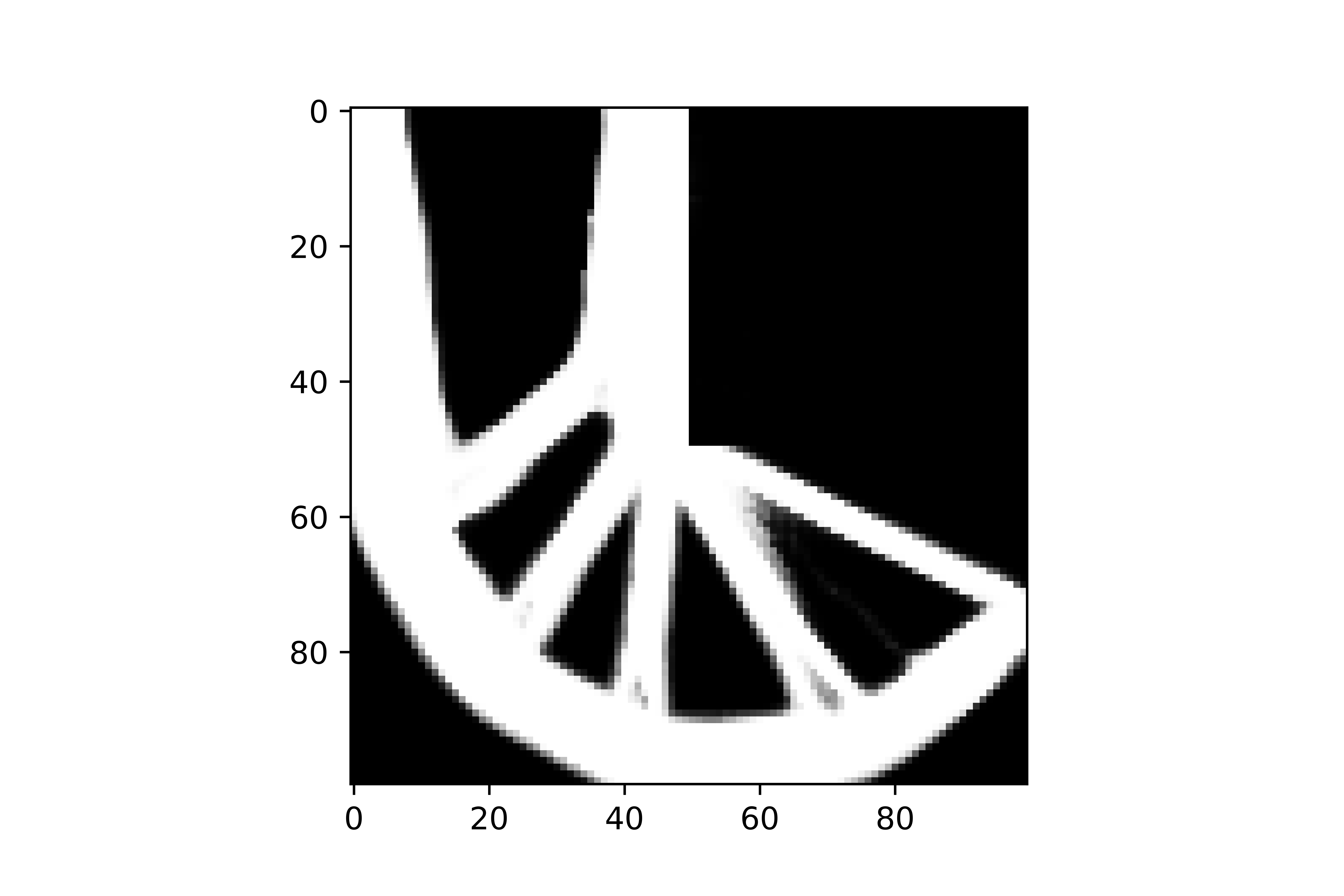
(d) Best design through gradient descent for $n_{\text{train}}=200$, $Q_{\text{rob}}=71.74$

(e) Best design via gradient descent for $n_{\text{train}}=600$, $Q_{\text{rob}}=69.84$

Figure 9: Comparison of the most optimal designs through various sources

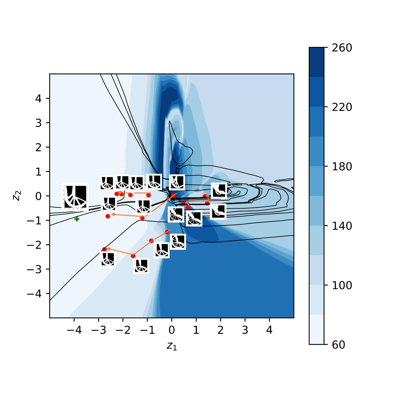
(a) Contour plot of compliance distribution

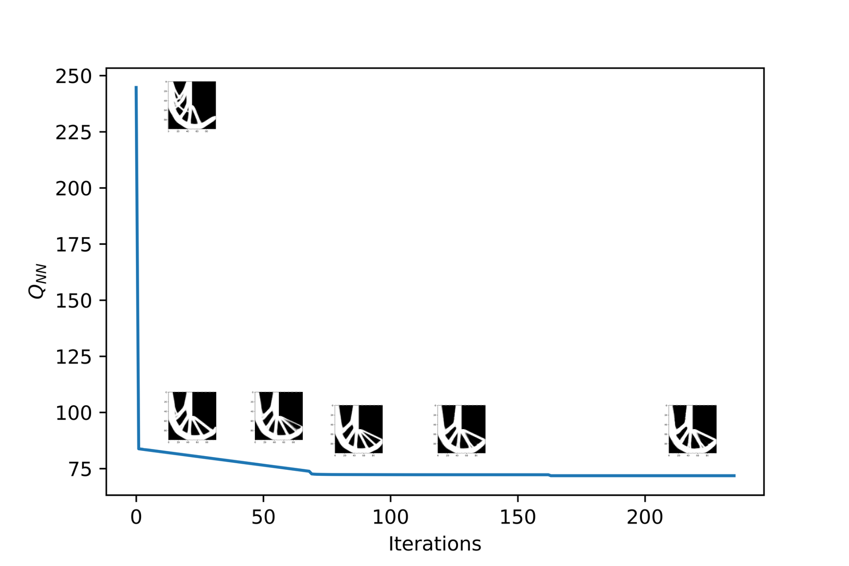
(b) Gradient descent evolution to the optimal design

Figure 10: Figure (a) shows a contour plot of robust compliance values in the latent space for $|\bm{z}|=2$ along with the gradient descent evolution of the designs from multiple starting points. The + sign indicates the location of the (global) optimal design. It can be observed that gradient descent could lead to local minima for certain starting points. Starting with a good $\bm{z}$ value can avoid falling into local minima. Figure (b) shows the gradient descent evolution from the starting image to the best design.

4.2 Heat Sink with loading uncertainty

The objective of the robust topology optimization of a heat conduction problem, in this study, is to minimize the robust thermal compliance, when subjected to distributed heating and includes one heat sink with fixed location and has varying load magnitude (i.e. heat source) [63]. The design domain for this problem is shown in Figure 11.

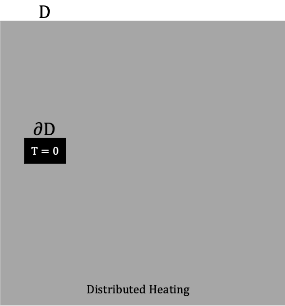
Figure 11: The design domain for the topology optimization of heat conduction problem.

The thermal compliance is calculated by solving the governing equation for the steady state heat conduction problem which can be re-written as

$$-\nabla(\mathbb{K}(\bm{x})\nabla T(\bm{x})) =f(\bm{x}),\,\,\, \forall\bm{x}\in D,$$ (10)

$$T(\bm{x}) =0,\ \ \ \forall\bm{x}\in\partial D,$$

where $D$ is the design domain, $\mathbb{K}$ is the thermal conductivity matrix, $f(\bm{x})$ is the given force function, and $T(\bm{x})$ is the temperature function. The temperature is calculated by solving the following finite element equilibrium equation

$$\bm{F}=\bm{K}\bm{T},$$ (11)

where $\bm{F}$ is the heat load vector, $\bm{K}$ is the symmetric heat conductivity matrix and $\bm{T}$ is the nodal temperature vector. Here, the load vector is parameterized with $\bm{F}=\bm{F}_{x}\cos(\xi)+\bm{F}_{y}\sin(\xi)$ where $\xi\sim U[0,\pi/2]$ is a uniform random variable, as the single source of uncertainty. The two deterministic coefficients $\bm{F}_{x}\in\mathbb{R}^{(n_{x}+1)^{2}}$ and $\bm{F}_{y}\in\mathbb{R}^{(n_{y}+1)^{2}}$ are set by drawing independent uniform realizations in each pixel. The deterministic thermal compliance is calculated as

$$Q(\bm{\theta})=\bm{F}^{T}\bm{T},$$ (12)

where $\bm{\theta}$ denotes the topology of the heat sink. The robust thermal compliance, $Q_{\text{rob}}$ is calculated using

$$Q_{\text{rob}}(\bm{\theta})=\mu_{\text{Q}}+\lambda\text{Var}_{\text{Q}}^{1/2},$$ (13)

where $\mu_{\text{Q}}$ and $\text{Var}_{\text{Q}}$ are the mean and variance of the deterministic thermal compliance vector. Thus, the robust topology optimization for the heat conduction problem can be written as

$$\underset{\bm{\theta}}{\text{minimize}} \mathrm{Q}_{\text{rob}}(\bm{\theta})$$ (14)

subject to $$\frac{V(\bm{\theta})}{V_{\text{0}}}=\alpha_{\text{v}}$$

$$0<\bm{\theta}_{\text{min}}\leq\bm{\theta}\leq 1.$$

In order to solve the robust thermal compliance minimization, the VAE is trained using a sample pool of 800 images of resolution $128\times 128$. Two additional hidden layers are added to the encoder and decoder networks of the previous example. The compliance neural network surrogate also has two additional hidden layers compared to that of L-bracket problem, to account for the increased resolution of the input images. Figure 12 shows a set of heat sink candidate designs randomly generated by the decoder part of the trained VAE.

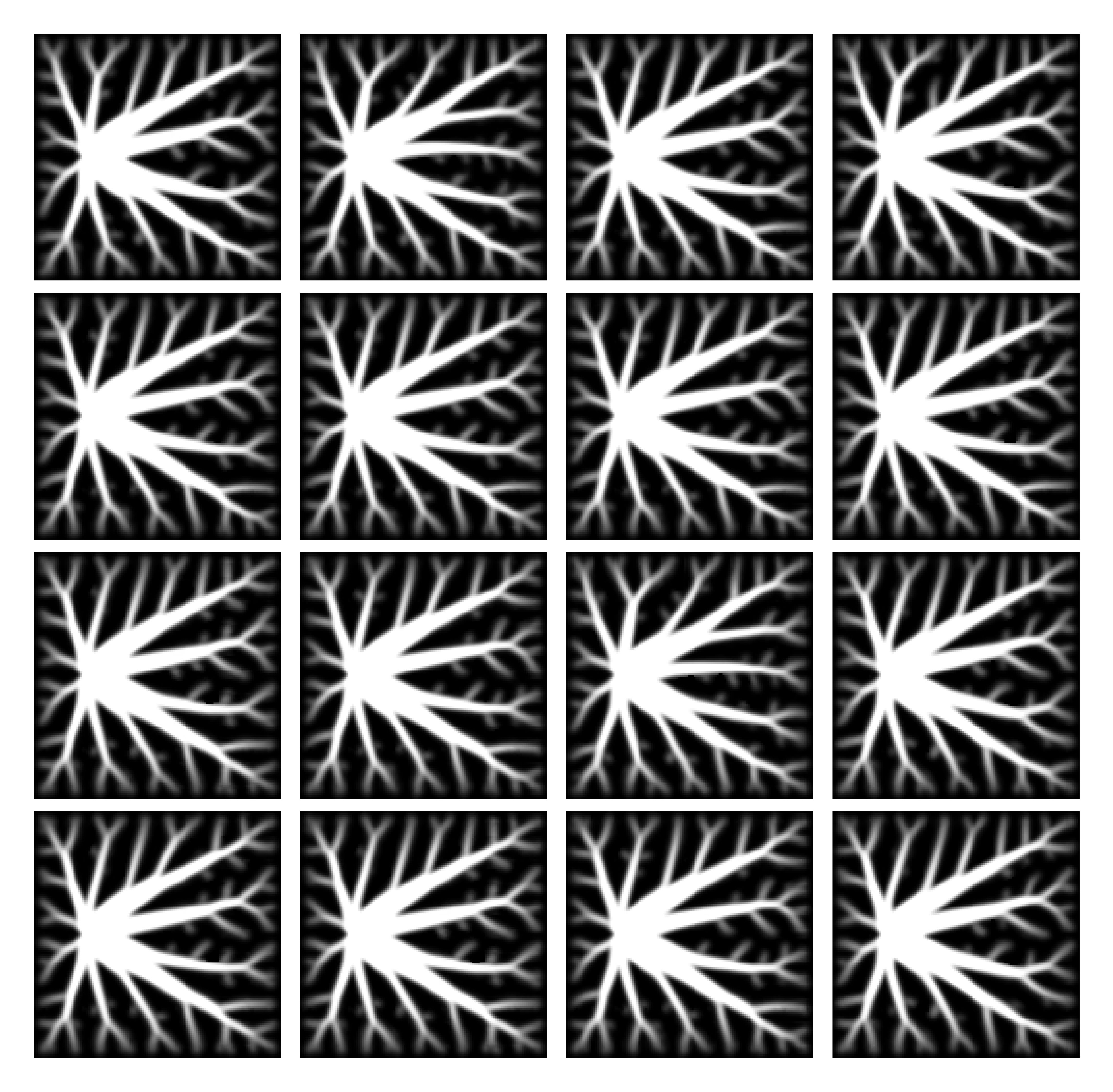
Figure 12: A sample of images generated by sample z values with $|\bm{z}|=2$ from standard normal distribution for $n_{train}=800$. The sampled z values are fed into the the decoder part of the VAE to generate these images.

Once the VAE and compliance neural networks are trained, we use the unconstrained optimization problem 9 via a gradient descent approach to find the optimal design for the heat sink. Figure 13 shows the trajectories of robust compliance and the corresponding initial and final designs. In this figure, we compare the solution from VAE with that from a finite element-based approach with the same initial topology. The robust compliance values are calculated using the quadrature method, similar to that of the L-bracket problem. It can be observed that gradient descent converges much faster (in less than 10 iterations) than finite element solution and is able to produce an optimal design with a lower robust compliance. Figure 14 shows the comparison of the best design found in the training set and the optimal design found via gradient descent algorithm. It can be observed that gradient descent gives a better design, in terms of robust compliance, compared to the samples in the training data. This is in accordance with our observations from the L-bracket example.

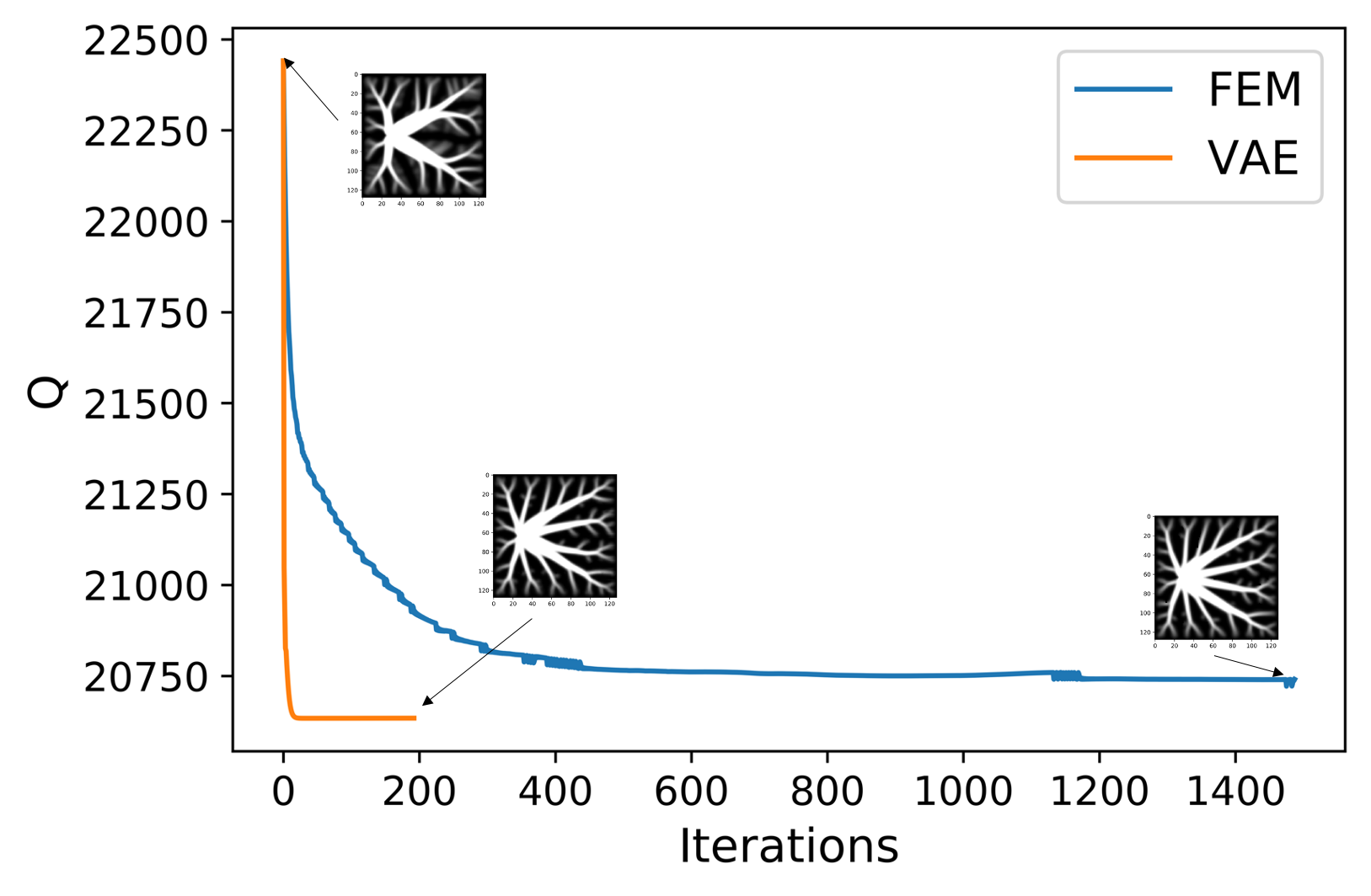
Figure 13: The evolution of the robust compliance via the gradient descent and the quadrature approach towards the optimal design for heat sink, using from the same starting image.

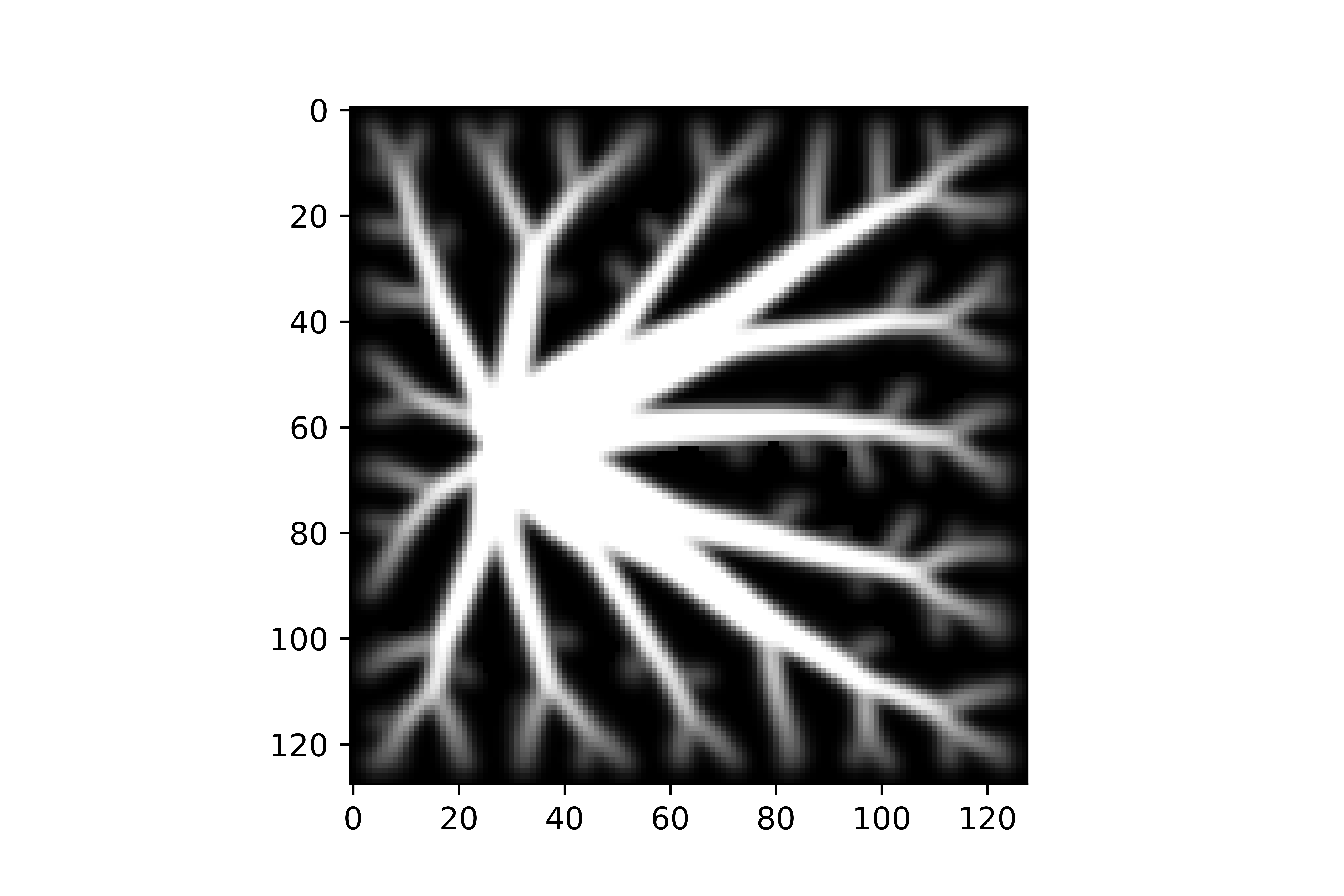
(a) Best design from training data, $Q=20,715$

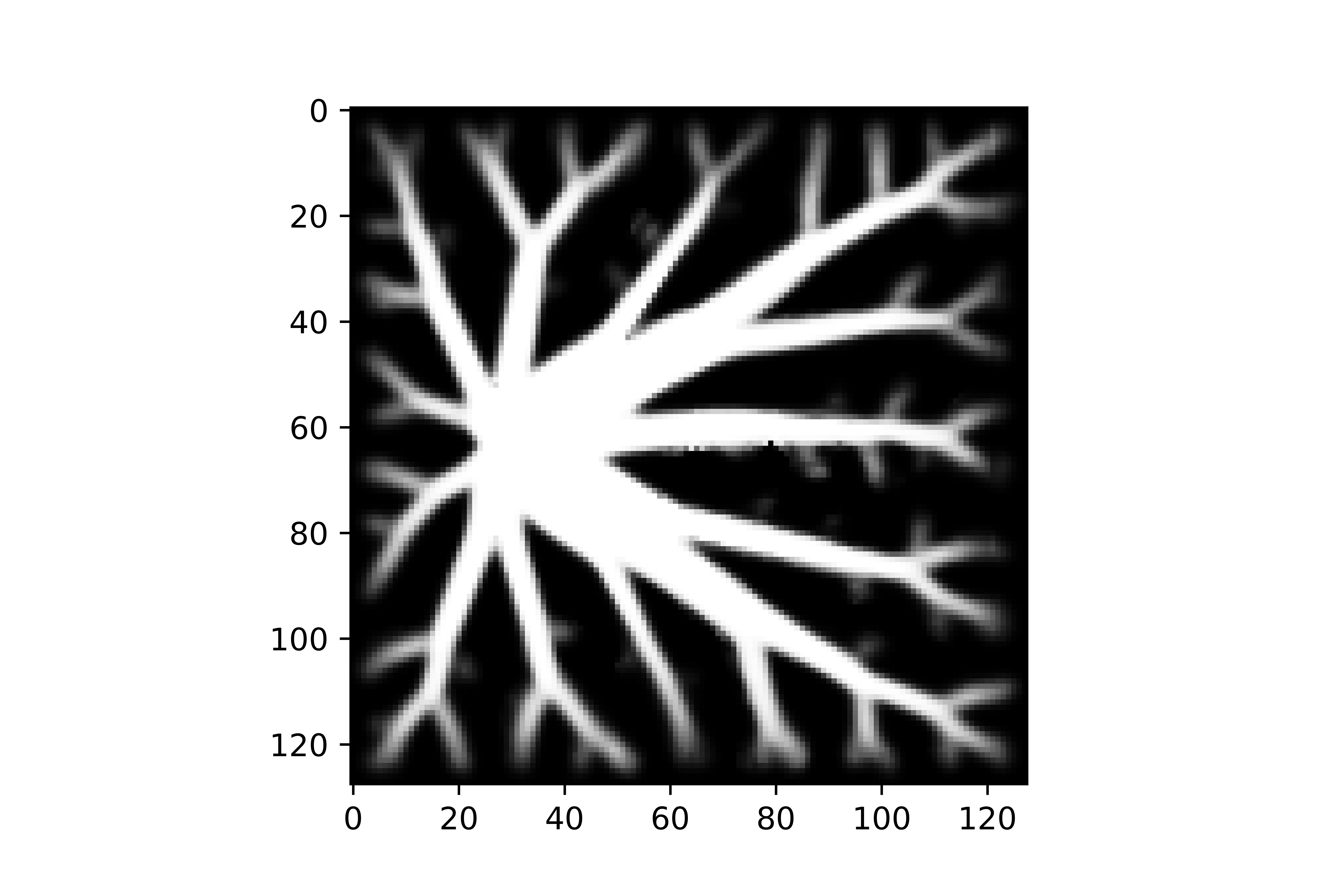
(b) Best design through gradient descent, $Q=20,637$

Figure 14: The identified designs for the heat sink.

5 CONCLUSION

Input uncertainties and computational challenges inherent in topology optimization approaches using finite element solvers motivate the utilization of deep learning algorithms to replace the bottle neck steps of the optimization process. In this paper, we studied how deep learning based techniques and neural networks can be used for an efficient parametrization of design topologies and also to provide an approximate forward model for the evaluation of robust compliance that can be easily differentiated and used in a gradient-based optimization. Using two examples, we highlighted how the proposed approach can offer computational efficiency with high accuracy. An important advantage of using deep learning in shape parametrization is its capability for automatic feature engineering/detection, using minimal amount of training data. This removes the need to explicitly impose the design constraints, such as volume fraction, in the loss function.

In this work, we used VAEs to turn the high dimensional optimization problem into a low dimensional one. Even though VAE was able to produce better designs than the training data, we could conclude that it can produce a robust optimal design that is better than what a finite element approach offers. The reason is that the quality of our optimal design is dependent on the search subspace, informed by the training data, which are the designs obtained from the deterministic optimization problem with different loading realizations. It should be noted that if the actual robust design has topology features that lie outside the search subspace, our gradient based approach may have limitations in reaching that specific topology. Therefore, as a next step, we are exploring the use of sub-optimal designs from SIMP for the training and evaluating if they can produce a design closer to the robust optimal design given the design constraints. This also points at the need for lower reliance on the training data for design generation. To this end, we are studying how we can replace a data driven neural network with a physics informed neural network, where design generation would be based on the governing physical equations, along with minimal training data. The other extensions to this work to be addressed in the future studies are (1) evaluating the structural integrity of the optimal design from the gradient descent process; and (2) incorporating the design constraints of the optimization problem in the neural network architecture.

References

- [1] Sigmund, Ole and Bondsgc, M.P. Topology optimization. State-of-the-Art and Future Perspectives, Copenhagen: Technical University of Denmark (DTU), 2003
- [2] De, S., Hampton, J., Maute, K., Doostan, A. Topology Optimization under Uncertainty using a Stochastic Gradient-based Approach. ArXiv, 1902.04562, 2019.
- [3] Keshavarzzadeh, V., Fernandez, F., Tortorelli, D.A. Topology optimization under uncertainty via non-intrusive polynomial chaos expansion. Computer Methods in Applied Mechanics and Engineering, 318: 120-147, 2017.
- [4] Bendsøe, M.P., Kikuchi, N. Generating optimal topologies in structural design using a homogenization method. Computer Methods in Applied Mechanics and Engineering, 71(2):197-224, 1988.
- [5] Bendsøe, M.P. Optimal shape design as a material distribution problem. Structural optimization, 1:193-202, 1989.
- [6] Mlejnek, H.P. Some aspects of the genesis of structures. Structural Optimization, 5:64-69, 1992.
- [7] Zhou, M., Rozvany, G.I.N. The COC algorithm, Part II: Topological, geometrical and generalized shape optimization. Computer Methods in Applied Mechanics and Engineering, 89(1-3):309-336, 1991.
- [8] Allaire, G., Jouve, F., Toader, A. A level-set method for shape optimization. Comptes Rendus Mathematique, 334(12):1125-1130, 2002.
- [9] Allaire, G., Jouve, F., Toader, A. Structural optimization using sensitivity analysis and a level-set method. Journal of Computational Physics, 194(1):363-393, 2004.
- [10] Wang, M.Y., Wang, X. Level Set Models for Structural Topology Optimization. DAC 2003, 2003.
- [11] Sokolowski, J., Żochowski, A. On the Topological Derivative in Shape Optimization. SIAM Journal on Control and Optimization, 37(4):1251-1272, 1999.
- [12] Bourdin, B., Chambolle, A. Design-Dependent Loads in Topology Optimization. ESAIM: Control, Optimisation and Calculus of Variations, 9:19-48, 2003.
- [13] Xie, Y.M., Steven, G.P. A simple evolutionary procedure for structural optimization. Computers & Structures, 49(5):885-896, 1993.
- [14] Rozvany, G.I.N., Zhou, M., Birker, T. Generalized shape optimization without homogenization. Structural Optimization, 4:250-252, 1992.
- [15] Dunning, P.D., Kim, H.A., Mullineux, G. Introducing loading uncertainty in topology optimization. AIAA Journal, 49 (4): 760-768, 2011.
- [16] Guest, J.K., Igusa, T. Structural optimization under uncertain loads and nodal locations. Computer Methods in Applied Mechanics and Engineering, 198(1): 116-124, 2008.
- [17] Guo, X., Zhang, W., Zhang, L. Robust structural topology optimization considering boundary uncertainties. Computer Methods in Applied Mechanics and Engineering, 253(1): 356-368, 2013.
- [18] Chen, S., Chen, W., Lee, S. Level set based robust shape and topology optimization under random field uncertainties. Structural and Multidisciplinary Optimization, 41: 507-524, 2010.
- [19] Beyer, H., Sendhoff, B. Robust optimization – A comprehensive survey. Computer Methods in Applied Mechanics and Engineering, 196(33-34): 3190-3218, 2007.
- [20] Guo, X., Bai, W., Zhang, W., Gao, X. Confidence structural robust design and optimization under stiffness and load uncertainties. Computer Methods in Applied Mechanics and Engineering, 198(41): 3378-3399, 2009.
- [21] Tootkaboni, M., Asadpoure, A., Guest, J.K. Topology optimization of continuum structures under uncertainty–a polynomial chaos approach. Computer Methods in Applied Mechanics and Engineering, 201: 263-275, 2012.
- [22] Chen, S., Chen, W. A new level-set based approach to shape and topology optimization under geometric uncertainty. Structural and Multidisciplinary Optimization, 44(1): 1-18, 2011.
- [23] Lazarov, B.S., Schevenels, M., Sigmund, O. Topology optimization with geometric uncertainties by perturbation techniques. International Journal for Numerical Methods in Engineering, 90(11): 1321-1336, 2012.
- [24] Kharmanda , G., Olhoff , N., Mohamed , A. Reliability-based topology optimization. Structural and Multidisciplinary Optimization, 26: 295-307, 2004.
- [25] Allen, M., Raulli, M., Maute, K., Frangopol, D.M. Reliability-based analysis and design optimization of electrostatically actuated MEMS. Computers & Structures, 82(13-14): 1007-1020, 2004.
- [26] Frangopol, D.M., Maute, K. Life-cycle reliability-based optimization of civil and aerospace structures. Computers & Structures, 81(7): 397-410, 2003.
- [27] Jung, H., Cho, S. Reliability-based topology optimization of geometrically nonlinear structures with loading and material uncertainties. Finite Elements in Analysis and Design, 41(3): 311-331, 2004.
- [28] Mozumder, C., Patel, N., Tillotson, D., Renaud, J., Tovar, A. An Investigation of Reliability-Based Topology Optimization. Session: MAO-28: Weight Management for Complex Systems, 2006.
- [29] Valdebenito, M.A., Schuëller, G.I. A survey on approaches for reliability-based optimization. Structural and Multidisciplinary Optimization, 42: 645-663, 2010.
- [30] Ates, G.C., Gorguluarslan, R.M. Two-stage convolutional encoder-decoder network to improve the performance and reliability of deep learning models for topology optimization. Structural and Multidisciplinary Optimization, 63: 1927–1950, 2021.
- [31] De, S., Maute, K., Doostan, A. Reliability-based Topology Optimization using Stochastic Gradients. 2021.
- [32] Diab, W.A., Koric, S., Sobh, N.A. Topology optimization of 2D structures with nonlinearities using deep learning. 2020.
- [33] Watts, S., Arrighi, W., Kudo, J., Tortorelli, D.A., White, D.A. Simple, accurate surrogate models of the elastic response of three-dimensional open truss micro-architectures with applications to multiscale topology design. Structural and Multidisciplinary Optimization, 60 : 1887-1920, 2019.
- [34] Oh, S., Jung, Y., Kim, S., Lee, I., Kang, N. Deep Generative Design: Integration of Topology Optimization and Generative Models. Journal of Mechanical Design, 141(11):1, 2019.
- [35] Banga, S., Gehani, H., Bhilare, S., Patel, S., Kara, L. 3D Topology Optimization using Convolutional Neural Networks. arXiv:1808.07440, 2018.
- [36] Cang, R., Yao, H., Ren, Y. One-shot generation of near-optimal topology through theory-driven machine learning. Computer-Aided Design, 109: 12-21, 2019.
- [37] Liu, C., Du, Z., Zhang, W., Guo, X. Machine Learning-Driven Real-Time Topology Optimization Under Moving Morphable Component-Based Framework. Journal of Applied Mechanics, 86:011004, 2019.
- [38] Sosnovik, I., Oseledets, I. Neural Networks for Topology Optimization. arXiv:1709.09578, 2017.
- [39] Yu, Y., Hur, T., Jung, J., Jang, I.G. Deep learning for determining a near-optimal topological design without any iteration. Structural and Multidisciplinary Optimization, 59: 787–799, 2019.
- [40] Burnap, A., Liu, Y., Pan, Y., Lee, H., Gonzalez, R., Papalambros, P.Y. Estimating and exploring the product form design space using deep generative models. ASME 2016 International Design Engineering Technical Conferences and Computers and Information in Engineering Conference, ACM, V02AT03A013- V02AT03A013, 2016.
- [41] Umetani, N. Exploring generative 3D shapes using autoencoder networks. SIGGRAPH Asia 2017 Technical Briefs, ACM, 24, 2017.
- [42] Farimani, A.B., Gomes, J., Pande, V.S. Deep learning the physics of transport phenomena. arXiv:1709.02432, 2017.
- [43] Guo, X., Li, W., Iorio, F. Convolutional neural networks for steady flow approximation. In Proceedings of the 22nd ACM SIGKDD International Conference on Knowledge Discovery and Data Mining, ACM, 481-490, 2016.
- [44] Tompson, J., Schlachter, K., Sprechmann, P., Perlin, K. Accelerating eulerian fluid simulation with convolutional networks. In Proceedings of the 34th International Conference on Machine Learning, JMLR, 70:3424-3433, 2017.
- [45] Yang, Z., Li, X., Brinson, L.C., Choudhary, A.N., Chen, W., Agrawal, A. Microstructural materials design via deep adversarial learning methodology. Journal of Mechanical Design, 140(11):111416, 2018.
- [46] Cang, R., Li, H., Yao, H., Jiao, Y., Ren, Y. Improving direct physical properties prediction of heterogeneous materials from imaging data via convolutional neural network and a morphology-aware generative model. Computational Materials Science, 150: 212-221, 2018.
- [47] Cang, R., Xu, Y., Chen, S., Liu, Y., Jiao, Y., Ren, M.Y. Microstructure representation and reconstruction of heterogeneous materials via deep belief network for computational material design. Journal of Mechanical Design, 139(7):071404, 2017.
- [48] Burnap, A., Pan, Y., Liu, Y., Ren, Y., Lee, H., Gonzalez, R., Papalambros, P.Y. Improving design preference prediction accuracy using feature learning. Journal of Mechanical Design, 138(7): 071404, 2016.
- [49] Gu, G.X., Chen, C.T., Buehler, M.J. De Novo Composite Design Based on Machine Learning Algorithme. Extreme Mech. Lett., 18:19-28, 2018.
- [50] Ulu, E., Zhang, R.S., Kara, L.B. A Data-Driven Investigation and Estimation of Optimal Topologies Under Variable Loading Configurations. Comput. Method Biomech.: Imaging Visualization, 4(2):61-72, 2016.
- [51] Guo, T., Lohan, D.J., Allison, J.T. An Indirect Design Representation for Topology Optimization Using Variational Autoencoder and Style Transfer. Structures, Structural Dynamics, and Materials Conference, 2018.
- [52] Understanding Variational Autoencoders (VAEs) https://towardsdatascience.com/understanding-variational-autoencoders-vaes-f70510919f73
- [53] SIMP methodology for topology optimization. http://help.solidworks.com/2019/english/solidworks/cworks/c_simp_method_topology.htm
- [54] Sigmund, O. A 99 line topology optimization code written in Matlab. Structural and Multidisciplinary Optimization, 21: 120-127, 2001.
- [55] Zhifang, F., Junpeng, Z., Chunjie, W. Robust Topology Optimization under Loading Uncertainty with Proportional Topology Optimization Method. Eighth International Conference on Measuring Technology and Mechatronics Automation (ICMTMA), Macau, 584-588, 2016.
- [56] Nabian, M.A., Meidani, H. A Deep Neural Network Surrogate for High-Dimensional Random Partial Differential Equations. Probabilistic Engineering Mechanics, 57: 14-22, 2019.
- [57] Wang, Y., Yao, H., Zhao, S. Auto-encoder based dimensionality reduction. Neurocomputing, 184: 232-242, 2016.
- [58] Goodfellow, I., Bengio, Y., Courville, A. Deep Learning MIT Press, 499-523, 2016.
- [59] Doersch, C. Tutorial on Variational Autoencoders. arXiv:1606.05908, 2016.
- [60] Kingma, D. P., Welling, M. An Introduction to Variational Autoencoders. Foundations and Trends in Machine Learning: 12(4) : 307-392, 2019.
- [61] Salunke, N.P., Juned Ahamad, R. A., Channiwala, S.A. Airfoil Parameterization Techniques: A Review. American Journal of Mechanical Engineering, 2(4): 99-102, 2014.
- [62] Andreassen, E., Clausen, A., Schevenels, M., Lazarov, B.S., Sigmund, O. Efficient topology optimization in MATLAB using 88 lines of code. Structural and Multidisciplinary Optimization, 43: 1-16, 2011.
- [63] Keshavarzzadeh, V., Alirezaei, M., Tasdizen, T., Kirby, R. M. Image-Based Multi resolution Topology Optimization Using Deep Disjunctive Normal Shape Model. Computer-Aided Design, 130 : 102947, 2020.