Non-locality of the Turbulent Electromotive Force

Abstract

The generation of large-scale magnetic fields ($\overline{\mathbf{B}}$) in astrophysical systems is driven by the mean turbulent electromotive force ($\overline{\mbox{\boldmath${\cal E}$}{}}$), the cross correlation between local fluctuations of velocity and magnetic fields. This can depend non-locally on $\overline{\mathbf{B}}$ through a convolution kernel $K_{ij}$. In a new approach to find $K_{ij}$, we directly fit the time series data of $\overline{\mbox{\boldmath${\cal E}$}{}}$ versus $\overline{\mathbf{B}}$ from a galactic dynamo simulation using singular value decomposition. We calculate the usual turbulent transport coefficients as moments of $K_{ij}$, show the importance of including non-locality over eddy length-scales to fully capture their amplitudes and that higher order corrections to the standard transport coefficients are small in the present case.

1 Introduction

A persistent theme applicable in many physical contexts is the influence of small-scale, or unresolved physics, on larger scales (Krause & Rädler, 1980; Bhat et al., 2016; Meneveau & Katz, 2000; Gotoh & Yeung, 2012; Aiyer et al., 2017; Baumann et al., 2012). This is also of crucial importance for understanding the origin of large-scale magnetic fields in stars and galaxies, ordered on scales larger than the turbulent motions. They are thought to be maintained by a mean field turbulent dynamo, through the combined action of helical turbulence and differential rotation. Their evolution is described by mean-field electrodynamics (Rädler, 1969; Moffatt, 1978; Krause & Rädler, 1980; Shukurov & Subramanian, 2021; Brandenburg & Subramanian, 2005), where the velocity field $\mathbf{U}$ and magnetic field $\mathbf{B}$ are decomposed as the sums of their mean or large-scale (with over-line) and fluctuating or small-scale parts, $\mathbf{U}=\overline{\mathbf{U}}+\mathbf{u}$ and $\mathbf{B}=\overline{\mathbf{B}}+\mathbf{b}$. The mean (or average) is often defined over a suitable domain such that the Reynolds’ averaging rules are satisfied. The evolution of $\overline{\mathbf{B}}$ is then determined by the averaged induction equation,

$$\frac{\partial\overline{\mathbf{B}}}{\partial t} =\nabla\times\left(\overline{\mathbf{U}}\times\overline{\mathbf{B}}+\overline{\mbox{\boldmath${\cal E}$}{}}-\eta_{m}\nabla\times\overline{\mathbf{B}}\right),$$ (1)

where $\eta_{m}$ is the microscopic diffusivity. Crucially, the generation of the large-scale or mean magnetic field (and its turbulent transport) is driven by a new contribution in Eq. (1), the mean turbulent electromotive force (EMF), $\overline{\mbox{\boldmath${\cal E}$}{}}=\overline{\mathbf{u}\times\mathbf{b}}$, which depends on the cross-correlation between the turbulent velocity and magnetic fields. The determination of $\overline{\mbox{\boldmath${\cal E}$}{}}$ in terms of the mean-fields themselves, either analytically using closure theory (Krause & Rädler, 1980; Pouquet et al., 1976; Dittrich et al., 1984; Shukurov & Subramanian, 2021; Blackman & Field, 2002; Rädler et al., 2003; Brandenburg & Subramanian, 2005) or in simulations, is the key to understand mean-field dynamos.

Several different approaches have been used so far to measure these coefficients directly from the MHD simulations in various contexts. Cattaneo & Hughes (1996), for instance, estimated the coefficients $\alpha_{ij}$, for a system in with uniform imposed mean magnetic field which generated the random magnetic fields. While Brandenburg & Sokoloff (2002) and Kowal et al. (2006), in an effort treat the additive noise in EMF more systematically, extracted these dynamo coefficients by fitting the various moments of magnetic fields (with EMF and themselves) with the data from direct simulations. Another method, developed for measuring the conductivity of solids, was adapted by Tobias & Cattaneo (2013) to determine the large-scale diffusivity of magnetic fields, in two-dimensional systems.

In a more systematic approach to estimate these coefficients at a fixed scale, the test-field method has also been developed (eg. Schrinner et al., 2005, 2007; Brandenburg, 2005). This method has now been used to extract the transport coefficients in various contexts, such as Supernova (SN) driven ISM turbulence, Convective turbulence in Solar and geodynamo simulations, accretion disc simulations etc. (eg. Gressel et al., 2008; Sur et al., 2008; Käpylä et al., 2009; Bendre et al., 2015; Gressel & Pessah, 2015; Bendre, 2016; Warnecke et al., 2018). The test-field method relies upon a notion that the fluctuating fields ($\mathbf{b}_{T}$) generated by a set of imposed passive test mean magnetic fields $\overline{\mathbf{B}}_{T}$ evolving with the turbulence ($\mathbf{u}$), contains all the information about dynamo coefficients. Components of the EMF associated with these test-fields ($\overline{\mathbf{u}\times\mathbf{b}_{T}}$) are then fitted with test-fields (and currents) to extract all the dynamo coefficients, at a scale of test magnetic fields. These $\mathbf{b}_{T}$ need to be reset to their initial values periodically to manage the exponentially growing noise in the determination of the transport coefficients.

Alternatively, a straightforward approach has been also adopted by Racine et al. (2011); Simard et al. (2016) where they fit the time series of EMF to those of mean-fields and currents using the singular value decomposition (SVD) algorithm, and obtain the dynamo coefficients in the simulations of convection driven stellar dynamos, as the least square solution. Advantage of such an approach (over the test-field) is that it depends on the actual magnetic fields from the simulations rather than a fixed-scale test-fields. A potential disadvantage is that the actual mean-fields are more noisy than the smooth "test-fields". In our earlier work (Bendre et al., 2020), we used this local SVD method on a galactic dynamo simulation and in Dhang et al. (2020) on a thick accretion disc simulation, with encouraging results. This motivates us to extend this method to also take the spatial non-locality of turbulent EMF into account.

This paper is structured as follows. In the following Sec.  2 we introduce both local and non-local turbulent transport coefficients. This is followed by Sec.  1 which describes the setup of direct numerical simulations (DNS) used in this work. The properties of the mean and fluctuating fields relevant for our analysis is outlined here and in Appendix  A. Sec.  4 describes the non-local SVD method for determining the transport coefficients. In Sec.  4 and Sec.  5 we discuss the outcomes of this analysis, followed by conclusions in Sec.  6.

2 Turbulent transport coefficients from $\overline{\mbox{\boldmath${\cal E}$}{}}$

A widely used local representation of the turbulent EMF, assumes that $\overline{\mbox{\boldmath${\cal E}$}{}}$ can be expanded in terms of the mean magnetic field and its derivative. In the current work, we use a planar, $xy$ average, to define mean-fields, and then the turbulent EMF can be written as

$$\overline{\mbox{\boldmath${\cal E}$}{}}_{i}(z,t)=\alpha_{ij}\overline{B}_{j}-\eta_{ij}\left(\nabla\times\overline{\mathbf{B}}\right)_{j}\,,$$ (2)

with the indices $i$ and $j$ representing either $x$ or $y$ components, and the mean-field having only a $z$ dependence. Here, $\alpha_{ij}$ and $\eta_{ij}$ are turbulent transport tensors. When Lorentz forces are small and in the isotropic limit, these tensors are diagonal; $\alpha_{ij}=\alpha_{0}\delta_{ij}$, $\eta_{ij}=\eta_{t}\delta_{ij}$. Then, in the limit of short correlation times, $\alpha_{0}$ or the $\alpha$ effect is proportional to the helicity of the turbulence and the turbulent diffusivity $\eta_{t}$ is proportional to its energy (Krause & Rädler, 1980; Brandenburg & Subramanian, 2005; Shukurov & Subramanian, 2021). Although, a number of different approaches have been used to estimate these coefficients even outside the isotropic limit, a majority assume this locality of the EMF. However, such an approximation is only valid when there is sufficient scale separation between the large-scale field and the turbulent velocity and ignores higher order derivatives of $\overline{B}_{i}$. In fact in disk galaxies, where the relevant ‘large’ scale is the height of the disk of order a few hundred  pc while the supernovae (SN) stirring scale is say 100 pc , the scale separation is very modest. This is mirrored in the simulations of the large-scale dynamo in the ISM (Bendre et al., 2015), where as we will see the scale of the mean-field is about 200 pc while the stirring scale is of order 50-100 pc . Thus it is important to decipher the range of validity of the locality assumption.

More generally $\overline{\mbox{\boldmath${\cal E}$}{}}$ can be be expressed in the form of a convolution with the mean-field itself (eg. Rädler, 1969; Brandenburg & Subramanian, 2005; Rädler, 2014; Brandenburg, 2018),

$$\overline{\mbox{\boldmath${\cal E}$}{}}_{i}\left(z,t\right)=\int_{-\infty}^{\infty}K_{ij}\left(z,\zeta,t\right)\,\overline{B}_{j}\left(z-\zeta,t\right)\,d\zeta\,.$$ (3)

This representation allows for the contribution of the mean magnetic field to the turbulent EMF in a non-local manner. For simplicity, we assume in this work that the time dependence is still local . Note that the convolution kernel $K_{ij}$ depends both on $z$ and a neighbourhood variable $\zeta$ separately, allowing for the inhomogeneity of magnetohydrodynamic turbulence in the general case. We will also see below that $K_{ij}$ falls off sufficiently rapidly with $\zeta$ that the limits of integration are effectively $\pm l/2$, where $l$ is order of the outer scale of turbulence. The more widely used local formulation, given by Eq. (2), can be recovered by Taylor expanding $\overline{B}_{j}$ in Eq. (3) about $z$, in powers of $\zeta$ and retaining the leading two terms.

$$\overline{\mbox{\boldmath${\cal E}$}{}}_{i}=\left(\int_{-\infty}^{\infty}K_{ij}(z,\zeta)\,d\zeta\right)\,\overline{B}_{j}(z)-\left(\int_{-\infty}^{\infty}K_{ij}\zeta\,d\zeta\right)\,\left(\frac{\partial\overline{B}_{j}}{\partial z}\right)_{\zeta=0}$$ (4)

Taking the solonoidity of mean-field into account, this allows the dynamo coefficients $\alpha_{ij}$ and $\eta_{ij}$ to be expressed in terms of the zeroth and first moments of $K_{ij}$ as

$$\begin{bmatrix}\alpha_{xx}&\alpha_{xy}\\ \alpha_{yx}&\alpha_{yy}\end{bmatrix}\ =\int^{+l/2}_{-l/2}\,\begin{bmatrix}K_{xx}&K_{xy}\\ K_{yx}&K_{yy}\end{bmatrix}\,d\zeta$$

$$\begin{bmatrix}\eta_{xx}&\eta_{xy}\\ \eta_{yx}&\eta_{yy}\end{bmatrix}\ =\int^{+l/2}_{-l/2}\,\begin{bmatrix}-K_{xy}&K_{xx}\\ -K_{yy}&K_{yx}\end{bmatrix}\,\zeta\,d\zeta\,.$$ (5)

Similarly, the subsequent higher order moments of the kernel multiply higher derivatives of $\overline{\mathbf{B}}$. The leading higher order corrections to $\alpha_{ij}$ which we denote by $\alpha^{h}_{ij}$ and $\eta_{ij}$ which we denote by $\eta^{h}_{ij}$ are,

$$\begin{bmatrix}\alpha^{h}_{xx}&\alpha^{h}_{xy}\\ \alpha^{h}_{yx}&\alpha^{h}_{yy}\end{bmatrix}= \int^{+l/2}_{-l/2}\begin{bmatrix}K_{xx}&K_{xy}\\ K_{yx}&K_{yy}\end{bmatrix}\zeta^{2}\,d\zeta$$

$$\begin{bmatrix}\eta^{h}_{xx}&\eta^{h}_{xy}\\ \eta^{h}_{yx}&\eta^{h}_{yy}\end{bmatrix}= \int^{+l/2}_{-l/2}\begin{bmatrix}-K_{xy}&K_{xx}\\ -K_{yy}&K_{yx}\end{bmatrix}\zeta^{3}\,d\zeta.$$ (6)

These multiply respectively the second and third derivatives of $\overline{B}_{j}$ in the Taylor expansion of Eq. (3). Our aim here is to compute $K_{ij}$ from the data of direct numerical simulations (DNS), examine the extent of its spatial non-locality and also derive in a novel manner, the dynamo coefficients as the moments of these components. For this we use a galactic dynamo simulation, (performed using the NIRVANA MHD code Ziegler (2008)), where supernovae (SN) introduced at randomly chosen points in the simulation box drive a multi-phase turbulent flow in the medium.

3 Description of the direct simulations

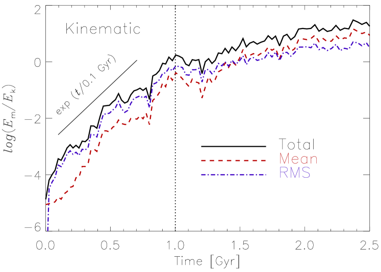
Figure 1: Time evolution of the various contributions of magnetic energy relative to (a nearly constant) turbulent kinetic energy is plotted here. Black-solid line corresponds to the total magnetic energy, red-dashed line the mean magnetic energy while the blue dot-dashed line shows the contribution of the fluctuating part of magnetic energy relative to the turbulent kinetic energy. The vertical dotted line delineates the kinematic from the dynamic phase of evolution and the slanted solid line shows the evolution expected for exponential growth of this energy ratio, for a growth rate of 100 Myr .

The details of the galactic dynamo simulations have been described in Bendre et al. (2015); Bendre (2016); Bendre et al. (2020); here we only summarize some features. Specifically, to have a reasonable comparison with the current determination of transport coefficients we use a run Q which has been analysed previously for this purpose using different methods, the test-field (TF) method (Bendre et al., 2015), a local linear regression method and a local version of the singular value decomposition (SVD) method (Bendre et al., 2020).

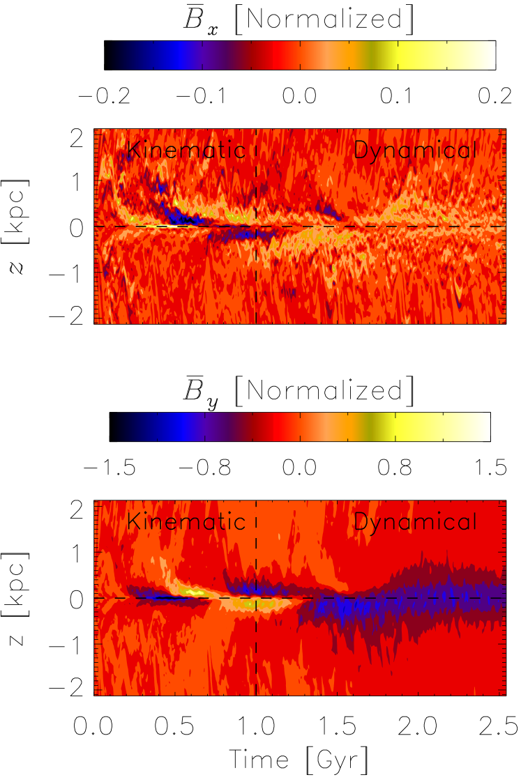
Figure 2: In the top panel we show the space-time evolution of the vertical profile of $\overline{{B}}_{x}$, along with a relevant color bar on the top. In the bottom panel the same is shown for the azimuthal component of $\overline{{B}_{y}}$. Color bars are normalized by the time-evolving square root of mean-field energy to scale out the growth of magnetic field components. Vertical dashed line mark roughly the end of initial kinematic phase, which can also be seen in Fig.  1.

The DNS model we use is a local Cartesian shearing box of ISM (with $L_{x}=L_{y}=0.8$ kpc , and -2.12 kpc to +2.12  kpc in the $z$ direction), split in $96\times 96\times 512$ grids with a resolution of $\sim 8.3$ pc . Shearing periodic boundary conditions are used in the radial ($x$) direction to incorporate the differential rotation. While the flat rotation curve is simulated by letting angular velocity scale as $\Omega\propto 1/R$ with the radius, with a value of $\Omega_{0}=100$  km s^-1  kpc ^-1 at the centre of the domain. In $z$ direction outflow conditions are used to let the gas escape, while preventing its inflow. Explicit values of kinematic viscosity ($5\times 10^{24}\rm{cm}^{2}\rm{s}^{-1}$) and magnetic diffusivity ($2\times 10^{24}\rm{cm}^{2}\rm{s}^{-1}$) are used to avoid having the dissipation controlled by the mesh itself, yielding a Prandtl number of the order of 2.5. SN explosions are simulated as expulsions of thermal energy at randomly chosen locations in the box at a rate of $\sim 7.5$ kpc ^-2 Myr ^-1. Furthermore the distribution of SN explosion locations is also scaled with the vertical profile of mass density. As an initial condition we use a vertically stratified density profile, such that the system is in a hydrostatic equilibrium, with a balance between gravitational and pressure gradient forces. This leads to a scale-height of $\sim 300$  pc for the density (and a midplane value of $10^{-24}$ g  cm^-3 ). Additionally, a piece-wise power law is also used to describe the temperature dependent radiative cooling. This, along with SN explosions, leads the plasma splitting into multiple thermal phases within a few  Myr , which roughly captures the ISM morphology.

The initial magnetic field is of a strength of about  $10^{-9}$ G  (about 3-4 orders of magnitude smaller than the equipartition strength). Both the total and mean magnetic field amplify exponentially with an e-folding time of $\sim 200$ Myr . The mean magnetic field goes through several reversals and parity changes until finally reaching to a large-scale mode vertically symmetric about the mid plane. Within about a $\,{\rm Gyr}\,$ they reach $\mu$G strengths, in equipartition with the turbulent kinetic energy density. Subsequently the magnetic energy continues to grow at about 5 times smaller growth rate. The time evolution of different magnetic energy density components and a space-time plot of $\overline{\mathbf{B}}(z,t)$ are shown in Fig.  1 and Fig.  2. The mean magnetic energy density and its space-time evolution, are also shown respectively in Fig. 9 and Fig. 10 of Bendre et al. (2020). An analysis of the properties of the fluctuating velocity and magnetic fields, relevant for understanding the extent of non-locality, is also given in Appendix  A

4 Determining the non-local kernel

To determine the components $K_{ij}$ using the SVD method we proceed as follows. We first extract the time series of $\overline{{B}}_{j}(z,t)$ and $\overline{\mbox{\boldmath${\cal E}$}{}}_{j}(z,t)=\overline{\left(\mathbf{u}\times\mathbf{b}\right)}_{j}$ at each $z$ and ranging from approximately 0 to 900 Myr in time, corresponding to the kinematic phase of the dynamo (comprising of 800 points in total). We then express Eq. (3) at any particular $z=z^{\prime}$ in the form of a discrete sum,

$$\overline{\mbox{\boldmath${\cal E}$}{}}_{i}(z^{\prime},t)=\sum_{n=-m}^{m}\,K_{ij}(z^{\prime},\zeta_{n},t)\,\overline{B}_{j}(z^{\prime}-\zeta_{n},t)\epsilon$$ (7)

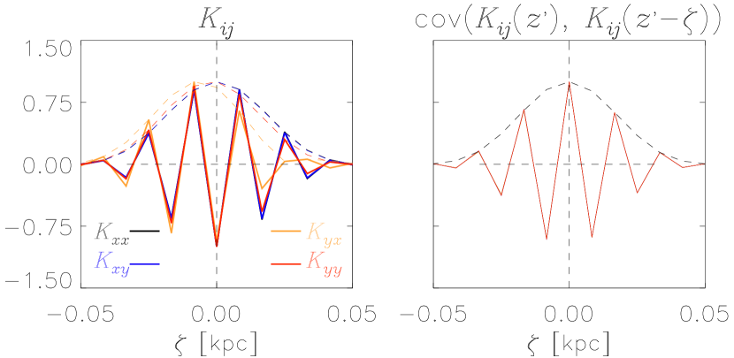
Figure 3: The left panel shows the normalized values of the convolution kernel $K_{ij}$ (solid lines) and its absolute value (dashed lines) at a representative $z^{\prime}=500$ pc . The right panel shows the normalized covariance of $K_{xx}$ (solid line) and its absolute value (dashed line) between the point $\zeta=0$ (also at $z^{\prime}=500$ pc ) and that at a neighbouring $\zeta$.

where $\zeta_{n}=n\epsilon$ denotes the location of mesh points in the local neighbourhood of and including $z^{\prime}$, with the index $n$ ranging from $-m$ to $+m$, and $\epsilon$ the size of the simulation mesh. The value of $m$ fixes the width of the local neighbourhood and it is expected that the coefficients $K_{ij}$ would vanish for a large enough $m$, such than $m\epsilon$ is larger than the eddy length-scales. We have explored vales of $m\leq 6$ equivalent of a local neighbourhood of about $-50$ to $50$ pc . This turns out to be sufficient as discussed below and seen from Fig.  3.

For $m=6$, Eq. (7) then represents a system of 2 equations in 26 unknowns (6 points on either sides of each $z=z^{\prime}$) which we solve by using a time series analysis. We assume that the coefficients $K_{ij}$ do not vary in time during the initial kinematic phase of the dynamo, when Lorentz forces are negligible which is justifiable as discussed in our previous analysis (Bendre et al., 2020). This allows us to express Eq. (7) at each $z=z^{\prime}$ and times $(t_{1},t_{2}\dots t_{N})$ as an over-determined system of linear equations between $\overline{\mbox{\boldmath${\cal E}$}{}}$ and $\overline{\mathbf{B}}$. To solve this system for $K_{ij}$ using SVD, we first write Eq. (7) in a matrix form, $\mathbf{y}_{i}=\mathbf{A}\cdot\mathbf{x}_{i}+\hat{\mathbf{n}}_{i}$ ($i$ is either $x$ or $y$), where the matrix $\hat{\mathbf{n}}_{i}$ represents an additive noise in the determination of the vector $\mathbf{y}_{i}$. Here

$$\centering\mathbf{y}_{i}^{\intercal}\@add@centering =\begin{bmatrix}\overline{\mbox{\boldmath${\cal E}$}{}}_{i}(z^{\prime},t_{1})&\overline{\mbox{\boldmath${\cal E}$}{}}_{i}(z^{\prime},t_{2})\ldots\overline{\mbox{\boldmath${\cal E}$}{}}_{i}(z^{\prime},t_{N})\end{bmatrix}$$

$$\mathbf{A}^{\intercal} =\begin{bmatrix}\overline{B}_{x}(z^{\prime}-6\epsilon,t_{1})&\overline{B}_{x}(z^{\prime}-6\epsilon,t_{2})&\ldots\overline{B}_{x}(z^{\prime}-6\epsilon,t_{N})\\ \vdots&\vdots&\vdots\\ \overline{B}_{x}(z^{\prime}+6\epsilon,t_{1})&\overline{B}_{x}(z^{\prime}+6\epsilon,t_{2})&\ldots\overline{B}_{x}(z^{\prime}+6\epsilon,t_{N})\\ \overline{B}_{y}(z^{\prime}-6\epsilon,t_{1})&\overline{B}_{y}(z^{\prime}-6\epsilon,t_{2})&\ldots\overline{B}_{y}(z^{\prime}-6\epsilon,t_{N})\\ \vdots&\vdots&\vdots\\ \overline{B}_{y}(z^{\prime}+6\epsilon,t_{1})&\overline{B}_{y}(z^{\prime}+6\epsilon,t_{2})&\ldots\overline{B}_{y}(z^{\prime}+6\epsilon,t_{N})\end{bmatrix}$$

$$\mathbf{x}_{i} =\begin{bmatrix}K_{ix}(z^{\prime},+6\epsilon)\\ \vdots\\ K_{ix}(z^{\prime},-6\epsilon)\\ K_{iy}(z^{\prime},+6\epsilon)\\ \vdots\\ K_{iy}(z^{\prime},-6\epsilon)\end{bmatrix}$$

and ${N=800}$ is the length of the time series. Furthermore, $\overline{\mathbf{B}}$ at the $m$ points outside the top and bottom of the boundaries is set to zero; however, adopting reflecting boundaries at the top and bottom, has negligible effect on the final results.

We find the least-square solution to the matrix relation $\mathbf{y}_{i}=\mathbf{A}\cdot\mathbf{x}_{i}+\hat{\mathbf{n}}_{i}$ by pseudo-inverting the design matrix $\mathbf{A}$ using the SVD algorithm. Specifically the matrix $\mathbf{A}$ is represented as a singular value decomposition $\mathbf{A}=\mbox{\boldmath${\cal U}$}{}\,\mathbf{w}^{-1}\,\mbox{\boldmath${\cal V}$}{}^{\intercal}$, where ${\cal U}$ and ${\cal V}$ are orthonormal matrices of dimension ($N\times 26$), and ($26\times 26$) while $\mathbf{w}$ is a $26\times 26$ diagonal matrix. The least-square solution, denoted by $\hat{\mathbf{x}}_{i}$, is then determined simply by, $\hat{\mathbf{x}}_{i}=\mbox{\boldmath${\cal V}$}{}\,\mathbf{w}\,\mbox{\boldmath${\cal U}$}{}^{\intercal}\,\mathbf{y}_{i}$ (Mandel, 1982; Press et al., 1992). Note that $\overline{\mbox{\boldmath${\cal E}$}{}}$ and $\overline{\mathbf{B}}$ grow exponentially as $\exp{(t/200{\rm Myr})}$ during the kinematic stage even as $K_{ij}$ remains constant. This growth is scaled out of $\mathbf{y}_{i}$ and the columns of $\mathbf{A}$ before implementing the SVD algorithm to find $\hat{\mathbf{x}}_{i}$, as in our earlier work (Bendre et al., 2020).

The SVD analysis also gives the full covariance matrix between the $l^{th}$ and $m^{th}$ element of $\hat{\mathbf{x}}_{i}$,

$$\mathrm{Cov}\Big{(}[\hat{\mathbf{x}}_{i}]_{l},\,[\hat{\mathbf{x}}_{i}]_{m}\Big{)} =\sum_{j=0}^{25}\frac{\mbox{\boldmath${\cal V}$}{}_{lj}\,\mbox{\boldmath${\cal V}$}{}_{mj}}{\mathbf{w}_{jj}^{2}}\,\sigma_{i}^{2}.$$ (8)

Here $\sigma_{i}$ is the $1\sigma$ variance associated the vector $\mathbf{y}_{i}$,

$$\sigma_{i}^{2}=\frac{1}{N}\left(\mathbf{y}_{i}-\mathbf{A}\hat{\mathbf{x}}_{i}\right)^{\intercal}\left(\mathbf{y}_{i}-\mathbf{A}\hat{\mathbf{x}}_{i}\right).$$ (9)

The diagonal ($l=m$) elements in Eq. (8) give the variance in the $l^{th}$ element in the vector of $\hat{\mathbf{x}}_{i}$ and so determines the $1\sigma$ errors in each component of the kernel $K_{ij}$. However, to determine the uncertainties in the various moments of the kernel (Eq. (5)), the fact that components $K_{ij}$ are correlated within the $\zeta$ neighbourhood also needs to be accounted for, and we use the square root of summation of SVD covariance matrix as a measure of uncertainty in the moments of kernel coefficients determined using least-square method. For example consider any of the turbulent transport coefficients, say $Z$, which is written as the sum $Z=\sum_{m=-6}^{6}z_{m}$. Then the variance $\mathrm{Var}(Z)=\sum_{m}\sum_{n}\mathrm{Cov}(z_{n},z_{m})$ and the measure of uncertainty in $Z$ can be calculated as $\sqrt{\mathrm{Var}(Z)}$.

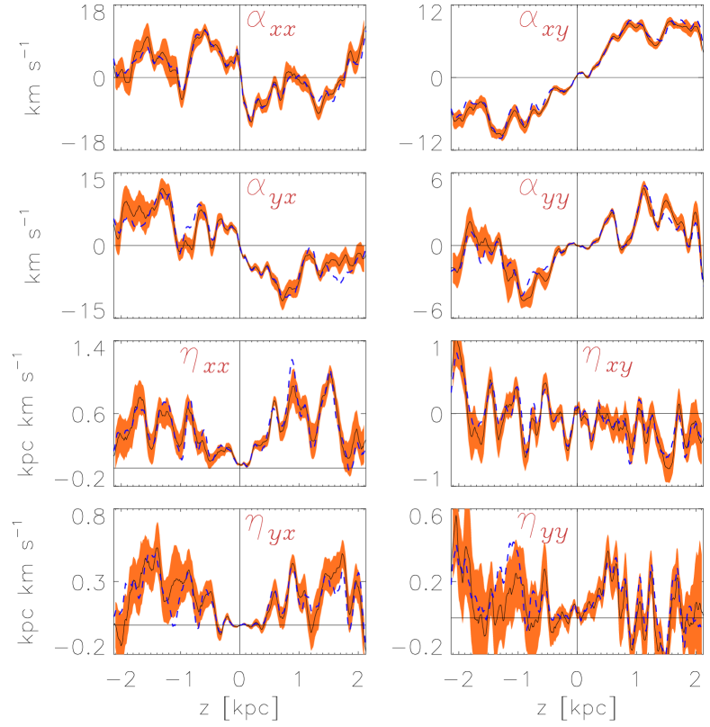
Figure 4: Blue-dashed lines show the vertical profiles of the zeroth and first moments of the kernel $K_{ij}$ calculated non-locally using Eq. (5) with the SVD method. We have adopted $m=6$, equivalent to the local neighbourhood of size $\pm 50$ pc . Shown in black-solid lines are the same profiles but calculated by applying the non-local SVD algorithm to nine different sections of time series $S_{1}$ to $S_{9}$ and averaging the outcomes. Orange shaded regions indicate a measure of uncertainty in these coefficients obtained from these realizations as described in the text.

In the left panel of Fig.  3 we show the normalized coefficients of the recovered convolution kernel $K_{ij}$ (solid lines) and their absolute values (dashed lines), as functions of $\zeta$ at a representative $z^{\prime}=500$ pc . We see that all coefficients drop to negligible values within $\zeta=\pm 50$ pc , which is also their approximate half widths. This scale is in fact of order of the correlation scale of interstellar medium turbulence in the simulations of Bendre et al. (2015) (see the discussion in Appendix  A) and also Hollins et al. (2017).

The right hand panel of Fig.  3 shows the normalised covariance (solid line) and its absolute value (dashed line) for $K_{xx}$, between its value at $\zeta=0$ (also at $z^{\prime}=500$ pc ) and that at an arbitrary neighbourhood point $\zeta$. Again, we see that these profiles too vanish smoothly at the boundaries of the chosen local neighbourhood. As the coefficients $K_{ij}(z^{\prime},\zeta)$ are correlated within the local neighbourhood, and determined only in the least-square sense, their amplitude at a particular $\zeta$ has correlated SVD variances. However, the extent of non-locality of $\overline{\mbox{\boldmath${\cal E}$}{}}$, is well constrained by the width of the dashed profiles in the left hand panel of Fig.  3.

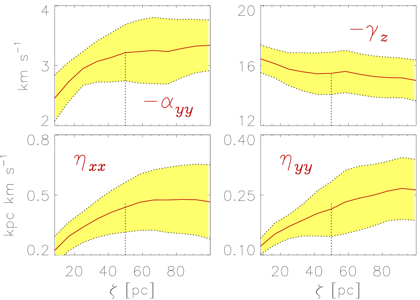
Figure 5: The solid red lines are various turbulent transport coefficients as functions of the half width of local neighbourhood (Fig.  4 corresponds to the width of 50 pc ). All the coefficients are averaged at the vertical location $z=1$ kpc $\pm 100$  pc , except for $\alpha_{yy}$ which is taken at $z=-1$ kpc $\pm 100$ pc , since its vertical profile has a fluctuation at around $\sim 0.8$  kpc , (eg. Fig.  4). Shaded in yellow are the regions corresponding to width of one mean absolute deviation. Dotted vertical lines at around 50 pc indicate the integral scale-length of turbulence.

5 turbulent transport coefficients

Once the kernel components $K_{ij}(z,\zeta)$ are determined, the transport coefficients $\alpha_{ij}$, $\eta_{ij}$, are obtained by calculating the first two moments of the kernel as in Eq. (5) after converting the integrals to discrete sums over $\zeta_{n}$ with $n$ ranging between $\pm m$. The vertical ($z$-dependent) profiles of these coefficients are shown in Fig.  4 as dashed lines. The SVD covariance in their determination, calculated from its variance as described above by summing over all the corresponding elements of the covariance matrix, turns out to be very small, less than $2-3\%$ of the coefficients themselves. This is both due to cancellations when summing over the signed covariances in $\sum_{m}\sum_{n}\mathrm{Cov}(z_{n},z_{m})$, and because the term $\sigma_{i}^{2}$ in Eq. (8) is small as it depends inversely on $N$. As an alternate direct estimate of uncertainty in these coefficients, we split the time series of $\overline{\mathbf{B}}$ and $\overline{\mbox{\boldmath${\cal E}$}{}}$ into nine different time series ($S_{1}$ to $S_{9}$) by extracting points that are about a correlation time apart (8 points in the time series) as in Bendre et al. (2020). We then use the SVD to determine $K_{ij}$ for each of these time series and compute its moments to determine $\alpha_{ij}$ and $\eta_{ij}$. The mean of these 9 realizations is shown as solid lines in Fig.  4 and it agrees well with that computed from the full series. The orange shaded regions in Fig.  4, indicate the square root of variance (in these nine realizations) divided by the number of realizations (see for example, Press et al. (1992)). We note that widening the size the of local neighbourhood amounts to the determination of more unknown $K_{ij}$’s in the system, which increases uncertainties in the determination of transport coefficients. Moreover, $\overline{\mbox{\boldmath${\cal E}$}{}}_{y}$ and $\overline{B}_{x}$ are noisier in the DNS compared to their counterparts, and therefore the coefficients $\alpha_{yx}$, $\eta_{xy}$ and $\eta_{yy}$, that depend on these two, are noisier compared to the other coefficients.

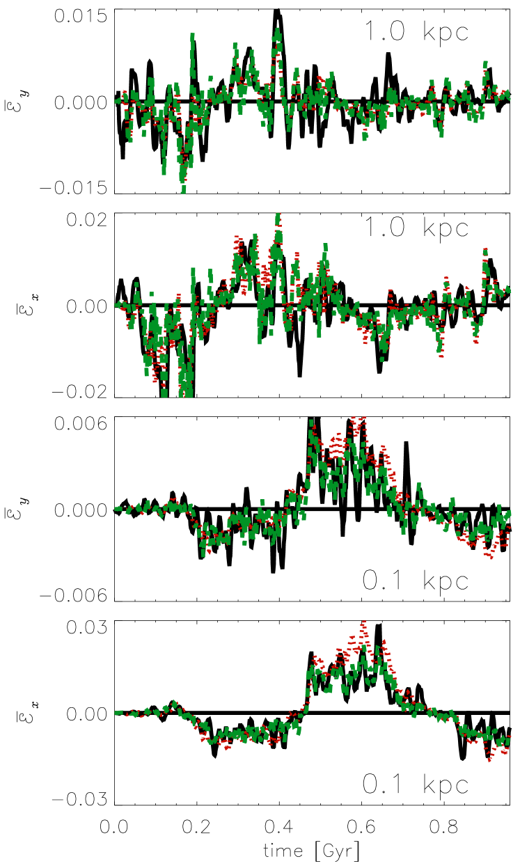
Figure 6: The black-solid lines show the time series of $x$ and $y$ components of EMF, as obtained from the DNS, at $z=1$ kpc (top two panels), while the bottom two panels show the same at $z=0.1$ kpc . The green-dashed lines show the same EMF time series but as reconstructed using Eq. (3), while the red-dotted lines show the EMF time series using only first two moments of the kernel (i.e. $\alpha_{ij}$ and $\eta_{ij}$). EMF components are expressed in the units of $\mu$ G  km s^-1 , and additionally we have scaled their time series with a factor $\exp{(-t/200{\rm Myr})}$ to account for the exponential growth of $\overline{\mbox{\boldmath${\cal E}$}{}}_{i}$.

The $z$-dependencies of turbulent coefficients in Fig.  4 are quite similar to their local determination in Bendre et al. (2020); however several of them, like $\eta_{ij}$ and $\alpha_{yy}$ have larger amplitudes. In fact we find that the vertical profiles of the dynamo coefficients determined adopting $m=1$ match very well with that determined from the same simulation using our previous local SVD analysis Bendre et al. (2020) (see e.g. Fig.  12(b)). To examine the importance of non-locality more carefully, we vary the size of local neighbourhood in Eq. (7), ranging from $m=1$ to 12 (about $\pm 8$ pc to $\pm 100$ pc ), and determine the components of $K_{ij}$ for each of those cases. The results are shown in Fig.  5 (as solid red lines), by averaging the coefficients at $z=1$ kpc $\pm 100$ pc , except for $\alpha_{yy}$ which is averaged over $z=-1$  kpc $\pm 100$ pc . Shaded in yellow are the regions corresponding to width of one mean absolute deviation. We see that $\alpha_{yy}$, crucial for the generation of $\overline{B}_{x}$ from $\overline{B}_{y}$, and the turbulent diffusion coefficients $\eta_{xx}$, $\eta_{yy}$ all increase with the size of neighbourhood until $m\sim 6$ (equivalent to $\sim\pm 50$ pc ), and stabilize thereafter (to the profiles shown in of Fig.  4). The turbulent diamagnetic pumping term $\gamma_{z}=(\alpha_{yx}-\alpha_{xy})/2$, which leads to a vertical advection of the mean-field also appears to stay constant with $m$ after initially decreasing up to $m\leq 6$. This indicates the importance of the non-local contributions included here, that are ignored when using Eq. (2) or too small a value of $m$ to compute the coefficients. The asymptotic values of these transport coefficients compare favorably with theoretical expectations for the galactic interstellar medium, and can lead to the large-scale dynamo action seen in this simulation, as already discussed in Bendre et al. (2020). The trends seen in Fig.  5 are also qualitatively consistent with Brandenburg et al. (2008); Rheinhardt & Brandenburg (2012b) and specifically the work of Gressel & Elstner (2020), where the scale dependence of the transport coefficients was obtained by varying the wave-number of test-fields (used to measure them) from $k=1$ (equivalent to the box size of $\sim 4$ kpc ) to $k=32$ (see also the discussion in Appendix  B). The present analysis, on the other hand, infers this dependence in a new direct approach by firstly using the actual mean-fields instead of test-fields, and also by increasing the width of the local neighbourhood, up from the grid size, to incorporate non-locality.

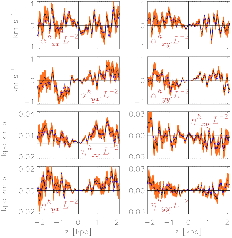
Figure 7: Shown in black-solid lines are vertical profiles of $\alpha^{h}_{ij}$ and $\eta^{h}_{ij}$ scaled with $L^{-2}$. These are determined by applying non-local SVD method to the time series $S_{1}$ to $S_{9}$, same as in the Fig.  4, and averaging the outcomes. Orange regions indicate the same measure of uncertainty as in Fig.  4. With blue-dashed lines same profiles are shown except they are calculated by taking the full time series into account.

Finally, in Fig.  6, we compare the time series of EMF components calculated directly from the DNS (black-solid line), with both the EMF reconstructed using Eq. (3) (and the recovered kernel coefficients $K_{ij}$) (green-dashed line), and also that using Eq. (2) (red-dotted line) which neglects higher order corrections to $\alpha_{ij}$ and $\eta_{ij}$. This is done at two representative locations. From Fig.  6, it is clear first that the non-local SVD method does indeed recover the EMF from the DNS reasonably well. Second, comparing the dashed and dotted lines in Fig.  6, we see that the inclusion of higher order terms does not significantly affect the determination of EMF, in the present galactic dynamo context. To see this explicitly, we compute $\alpha^{h}_{ij}$, and the hyper-diffusion correction $\eta^{h}_{ij}$ using Eq. (6) after converting it to discrete sums. In Fig.  7 we show these second and third moments of $K_{ij}$ in the same units as $\alpha_{ij}$ and $\eta_{ij}$. This has been done by dividing them by $L^{2}$, where $L=0.2$ kpc is of order of the scale over which the mean magnetic field varies. Note that we have not scaled these higher order coefficients by square of the integral scale of turbulence, since they get multiplied by the higher derivatives of mean magnetic field in the mean-field induction equation. It can be seen by comparing Fig.  7 with Fig.  4, that these higher order contributions are of order a few percent to ten percent of $\alpha_{ij}$ and $\eta_{ij}$. This can also be seen by comparing the $y$-range of the panels in these two figures. This is a small correction in the present case; however such contributions could be important in other contexts.

6 Conclusions

We have shown here that the turbulent EMF depends in a non-local manner on the mean magnetic field, and determined the corresponding non-local convolution kernel $K_{ij}(z,\zeta)$ which relates the two as in Eq. (3). This non-locality can emerge if there is only a modest scale separation between the scale of mean magnetic field and the driving scale, as obtains in both disk galaxies and in ISM simulations which realize a large-scale dynamo. We compute these non-local kernels using a new approach of least-square fitting directly the time-series data of the $\overline{\mbox{\boldmath${\cal E}$}{}}$ versus $\overline{\mathbf{B}}$, from a galactic dynamo simulation, using the SVD method. We show that the non-locality extends over eddy length-scales of order $\pm 50$ pc around any fiducial location and the reconstructed $\overline{\mbox{\boldmath${\cal E}$}{}}$ using Eq. (3) matches well with that obtained directly from the simulation. The lowest order moments of $K_{ij}$ over $\zeta$ give the standard local turbulent transport coefficients $\alpha_{ij}$ and $\eta_{ij}$, which however only converge when one accounts for the full extent of non-locality of $K_{ij}$. Higher order corrections to the standard transport coefficients are small in the present galactic dynamo simulation, but importantly, our method allows us to explicitly compute them. A caveat of the linear least-square fitting method using the SVD is that it requires $\mathbf{y}_{i}$ and $\mathbf{x}_{i}$ to vary over sufficiently large range (as in the present case). However, their advantages are many; of being able to use directly the simulation data without having to solve a set of auxiliary equations as in the test-field method, to handle additive noise $\hat{\mathbf{n}}$, and to determine the full covariance matrix of the of the fitted parameters. As we have shown here the method can also be generalized to determine the non-locality of transport coefficients. It would be of interest to test this method on other physical systems, not only in MHD and fluid turbulence but also in the context of any effective field theory, where subgrid physics affects larger scales.

Data Availability

The data underlying this article will be shared on reasonable request to the corresponding author.

Appendix A Properties of the ISM turbulence

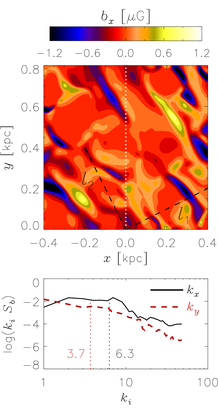
Figure 8: In the top panel we show contours of the $x$ component of fluctuating magnetic field with a corresponding color bar. While, in the bottom panel we plot the power per unit logarithmic interval in $k$-space of $\mathbf{b}$ as functions of $k_{x}$ with $k_{y}=1$ (black-solid line) and also as a function of $k_{y}$ with $k_{x}=1$ (red-dashed line). Vertical (dotted) lines below the curves indicate the average wavenumber of the spectra. The calculation is performed in 2 different directions since the field itself is anisotropic as can also be inferred from the contours.

It is of interest to determine the spectral and correlation properties of the turbulent velocity and magnetic fields which lead to the mean electromotive force. This will also aid in seeing the relevance of 50 pc scale appearing in the half widths of $K_{ij}(\zeta)$ and its connection to length-scales of the turbulence directly. We first analyze the two dimensional power spectra of $\mathbf{b}$ (and also for $\mathbf{u}$) over $xy$ planes at several different heights $z$. We define the power spectrum of a quantity $q(\boldsymbol{r})$ as,

$$S_{q}(k_{x},k_{y})=\left|\,\int_{\boldsymbol{r}}q(\boldsymbol{r})\exp{\left(-2\pi i\boldsymbol{k}\cdot\boldsymbol{r}\right)}\,d^{2}\boldsymbol{r}\,\right|^{2}$$ (10)

Where $\boldsymbol{r}$ is a vector in $xy$ plane, $\boldsymbol{k}$ a vector in $(k_{x},k_{y})$ plane and $q(\boldsymbol{r})$ can be any component of $\mathbf{b}(x,y)$ or $\mathbf{u}(x,y)$. The usual practice is then to define shell averaged 1-D spectra. However, the turbulence itself is anisotropic in the present case, due to the presence of differential shear. This may also be realized qualitatively just by noting the presence of elongated structures in the contours of both $b_{x}(x,y)$ and $u_{x}(x,y)$ shown in the top panels of Fig.  8 and Fig.  9 with two distinct integral-scales roughly along the direction shown by $l_{1}$ and $l_{2}$. Consequently, the power-spectra of $\mathbf{b}$ and $\mathbf{u}$ ($S_{b}$ and $S_{u}$, defined as the sum of the power spectra of their components) along these two directions yield different integral wave-numbers (larger along the direction of $l_{1}$). We show sections of the anisotropic 2-dimensional power spectrum of $\mathbf{b}$ and $\mathbf{u}$, in the bottom panels of Fig.  8 and Fig.  9 respectively. Specifically the solid lines show the power per unit logarithmic interval in $k$-space along $k_{x}$ with $k_{y}=1$ and the dashed lines along $k_{y}$ with $k_{x}=1$. This anisotropy is primarily the reason why refrain from computing the $k$-shell averaged power spectra over $(k_{x},k_{y})$ plane or the integral-scales using these power-spectra.

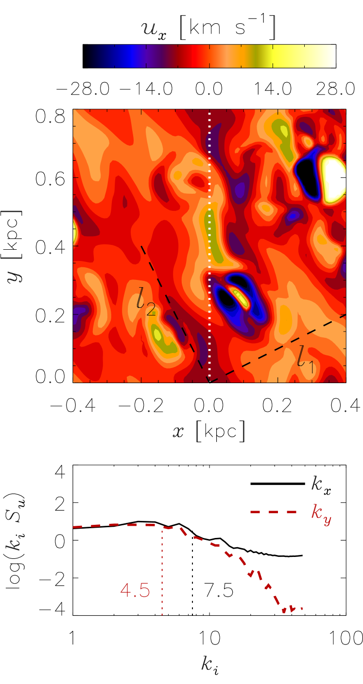
Figure 9: same as Fig.  8 but for $\mathbf{u}$

In order to compute the integral-scales of $\mathbf{b}$ and $\mathbf{u}$ along $l_{1}$ and $l_{2}$, we adopt an alternate approach. We calculate the two point correlation functions for $\mathbf{b}$ and $\mathbf{u}$ in $xy$ planes, $C_{b}$ and $C_{u}$, at various heights $z$, integral of which along any specific direction reflects the average correlation length-scale in that direction. The two point correlation function of $q(\boldsymbol{r})$ is given by the Fourier transform of the corresponding power-spectrum

$$C_{q}(\boldsymbol{R})=\,<q(\boldsymbol{r})\cdot q(\boldsymbol{r}^{\prime})>\,=\int_{\boldsymbol{k}}\,S_{q}(\boldsymbol{k})\exp{\left(2\pi i\boldsymbol{k}\cdot\boldsymbol{R}\right)}\,d^{2}\boldsymbol{k}\,,$$ (11)

where $\boldsymbol{R}=\boldsymbol{r}-\boldsymbol{r}^{\prime}$ is the relative position vector with components $(X,Y)$. Specifically, we define the correlation function of $\mathbf{b}$ to be $C_{b}(X,Y)=<\mathbf{b}(\boldsymbol{r})\cdot\mathbf{b}(\boldsymbol{r}^{\prime})>$ calculated by replacing $S_{q}$ in Eq. (11) by $S_{b}$, and correspondingly define $C_{u}(X,Y)$ for the velocity field $\boldsymbol{u}$. In the left hand panels of Fig.  10 and Fig.  11, we show as a contour plot, these correlations functions (normalized with respect to the value at origin), along with respective color bars. It can be seen that averaged correlation length (or the line integral of normalized correlation functions) along the direction $l_{1}$ and orthogonal direction $l_{2}$ are indeed different. In the bottom panel on the right hand side of each figure, we plot these correlation functions against length along $l_{1}$ (black-solid lines) and $l_{2}$ (red-dashed lines). We integrate the normalized $C_{b}$ and $C_{u}$ along $l_{1}$ and $l_{2}$ to compute the averaged correlation lengths in those directions and repeat this analysis at different heights ($z$). The top panel on the right-hand side (of Fig.  10 and Fig.  11) shows these averaged correlation lengths along $l_{1}$ (in black-solid lines) and $l_{2}$ in (red-dashed lines) as functions of $z$. They are $\sim 50$ pc and $\sim 100$ pc respectively, for both $\mathbf{b}$ and $\mathbf{u}$. This also yields magnetic Reynolds number $R_{m}$ of the order of 70-150 (the magnetic Prandtl number is $\sim 2.5$). A similar analysis is also performed to compute the correlation length-scales in the $z$ directions however assuming homogeneity in $z$ direction, despite the vertical stratification and they are $\sim 50$ pc , similar to that along $l_{1}$. These correlation lengths are consistent with the half widths of $K_{ij}(\zeta)$ inferred in Sec.  4 and the extent of non-locality in the transport coefficients found in Sec.  5.

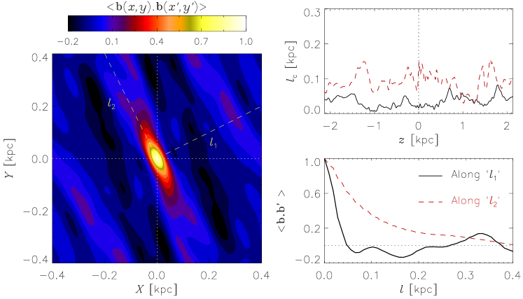
Figure 10: In the left hand panel we show the contour of the normalized 2-point correlation function $C_{b}(X,Y)/C_{b}(0,0)$, at $z=-0.8$ kpc , along with a corresponding color bar. Elliptical shape of the contour levels revels the statistical anisotropy of $\mathbf{b}$ due to shear. Integration of this function along a particular direction provides a correlation length-scale, $l_{c}$, along it. In the right hand lower panel we plot these normalized correlations along the direction $l_{1}$ (minor axis of the ellipse) with a black-solid line. While the red-dashed line indicates the same along the direction of $l_{2}$. In the upper half of right-hand panel these correlation lengths, along $l_{1}$ and $l_{2}$ are shown as the function of $z$, with a same color code.

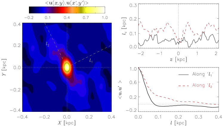
Figure 11: Same as Fig.  10 but for $\mathbf{u}$.

Appendix B Comparison with Test-Field and local SVD results

Data from the same model was also analysed with the test-field method previously and dynamo coefficients were obtained. Test-field which extends over the full $z$-extent of the simulation box (wavenumber $k=1$) was used in this analysis. The $z$ profiles of the coefficients thus obtained are presented in Fig.  12(a) for reference. To determine these, we have divided the kinematic phase (up to $\sim 1$ Gyr ) in nine independent time sections, and estimated the coefficients for each of these sections. Shown in Fig.  12(a) with black-solid lines are averages of these realizations, while the orange shaded regions correspond to the square root of the ratio of variance in these nine realizations and the number of realizations, determined the same way as in Fig.  4 and also in Press et al. (1992). Its comparison with the results from the local SVD method are discussed in Bendre et al. (2020).

As mentioned in Sec.  5 our non-local SVD calculations with a narrowest possible width of local neighborhood (with $m=1$, total 3 points) yield the same coefficients as from our local calculations. In Fig.  12(b) we plot these coefficients along with corresponding uncertainties in the determination. It appears that the coefficients $\alpha_{yy}(z)$ and $\gamma(z)$ are comparable with the outcomes of test-field method. The differences in the determination of other coefficients stem from the fact that the test-field method probes these coefficients at a fixed wavenumber of the test magnetic fields themselves, while in SVD the coefficients at all the scales spanned by mean fields are determined as a combination. Moreover, this set of coefficients does not uniquely determine the EMF and covariances associated with them, which we have discussed in Bendre et al. (2020).

Furthermore in Gressel & Elstner (2020), the authors have analyzed the scale dependence of dynamo coefficients by varying $k$, considering smaller test-field extent. They demonstrated that the smaller the scale of the test-field, the smaller the transport coefficients, approximately decreasing with $k$ as a Lorenztian. We note that the scale of the mean-field in the DNS is a few hundred  pc , which corresponds to larger $k$ and the test-field results are then consistent with our current non-local determination of these transport coefficients.

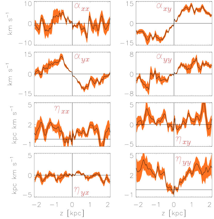
(a) Shown with black-solid lines are various dynamo coefficients for the same model as used in the main text, obtained using the test-field method, by dividing the whole time-series in nine sections and taking the averages of the outcomes. Shaded in orange are regions corresponding to uncertainties in these determinations obtained the same way as in Fig.  4

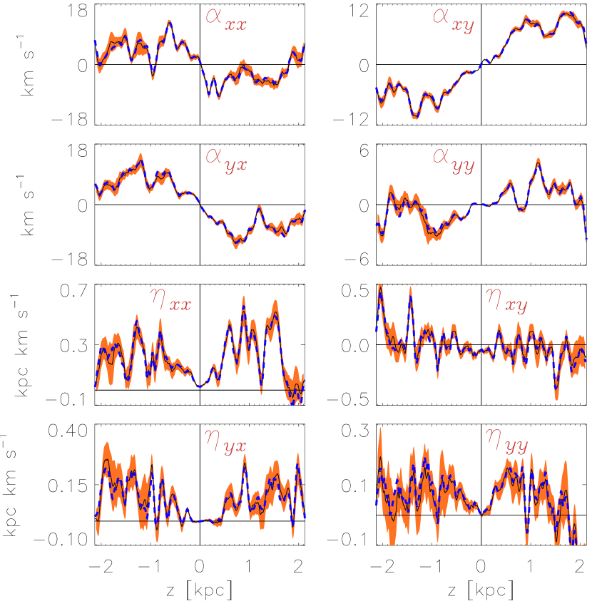
(b) Same as Fig.  4 but with $m=1$, i.e. three points in the local neighbourhood. The dashed-blue line indicate the same coefficients determined with our local version of SVD method discussed in Bendre et al. (2020).

References

- Aiyer et al. (2017) Aiyer A. K., Subramanian K., Bhat P., 2017, J. Fluid Mech., 824, 785
- Baumann et al. (2012) Baumann D., Nicolis A., Senatore L., Zaldarriaga M., 2012, Journal of Cosmology and Astroparticle Physics, 2012, 051
- Bendre (2016) Bendre A. B., 2016, doctoralthesis, Universität Potsdam
- Bendre et al. (2015) Bendre A., Gressel O., Elstner D., 2015, Astronomische Nachrichten, 336, 991
- Bendre et al. (2020) Bendre A. B., Subramanian K., Elstner D., Gressel O., 2020, MNRAS, 491, 3870
- Bhat et al. (2016) Bhat P., Subramanian K., Brandenburg A., 2016, MNRAS, 461, 240
- Blackman & Field (2002) Blackman E. G., Field G. B., 2002, Phys. Rev. Lett., 89, 265007
- Brandenburg (2005) Brandenburg A., 2005, Astronomische Nachrichten, 326, 787
- Brandenburg (2018) Brandenburg A., 2018, Journal of Plasma Physics, 84, 735840404
- Brandenburg & Sokoloff (2002) Brandenburg A., Sokoloff D., 2002, Geophys. Astrophys. Fluid Dyn., 96, 319
- Brandenburg & Subramanian (2005) Brandenburg A., Subramanian K., 2005, Physics Reports, 417, 1
- Brandenburg et al. (2008) Brandenburg A., Rädler K. H., Schrinner M., 2008, A&A, 482, 739
- Cattaneo & Hughes (1996) Cattaneo F., Hughes D. W., 1996, Phys. Rev. E, 54, R4532
- Dhang et al. (2020) Dhang P., Bendre A., Sharma P., Subramanian K., 2020, Monthly Notices of the Royal Astronomical Society, 494, 4854
- Dittrich et al. (1984) Dittrich P., Molchanov S. A., Sokoloff D. D., Ruzmaikin A. A., 1984, AN, 305, 119
- Gotoh & Yeung (2012) Gotoh T., Yeung P., 2012, Passive Scalar Transport in Turbulence: A Computational Perspective. Cambridge University Press, p. 87–131
- Gressel & Elstner (2020) Gressel O., Elstner D., 2020, MNRAS, 494, 1180
- Gressel & Pessah (2015) Gressel O., Pessah M. E., 2015, ApJ, 810, 59
- Gressel et al. (2008) Gressel O., Elstner D., Ziegler U., Rüdiger G., 2008, Astronomy and Astrophysics, 486, L35
- Hollins et al. (2017) Hollins J. F., Sarson G. R., Shukurov A., Fletcher A., Gent F. A., 2017, ApJ, 850, 4
- Hubbard & Brandenburg (2009) Hubbard A., Brandenburg A., 2009, ApJ, 706, 712
- Käpylä et al. (2009) Käpylä P. J., Korpi M. J., Brandenburg A., 2009, Astronomy and Astrophysics, 500, 633
- Kowal et al. (2006) Kowal G., Otmianowska-Mazur K., Hanasz M., 2006, A&A, 445, 915
- Krause & Rädler (1980) Krause F., Rädler K.-H., 1980, Mean-Field Magnetohydrodynamics and Dynamo Theory. Pergamon Press (also Akademie-Verlag: Berlin), Oxford
- Mandel (1982) Mandel J., 1982, The American Statistician, 36, 15
- Meneveau & Katz (2000) Meneveau C., Katz J., 2000, Annual Review of Fluid Mechanics, 32, 1
- Moffatt (1978) Moffatt H. K., 1978, Magnetic Field Generation in Electrically Conducting Fluids. Cambridge Univ. Press, Cambridge
- Pouquet et al. (1976) Pouquet A., Frisch U., Leorat J., 1976, J. Fluid Mech, 77, 321
- Press et al. (1992) Press W. H., Teukolsky S. A., Vetterling W. T., Flannery B. P., 1992, Numerical Recipes in C (2Nd Ed.): The Art of Scientific Computing. Cambridge University Press, New York, NY, USA
- Racine et al. (2011) Racine É., Charbonneau P., Ghizaru M., Bouchat A., Smolarkiewicz P. K., 2011, ApJ, 735, 46
- Rädler (1969) Rädler K.-H., 1969, Veroeffentlichungen der Geod. Geophys, 13, 131
- Rädler (2014) Rädler K. H., 2014, arXiv e-prints, p. arXiv:1402.6557
- Rädler et al. (2003) Rädler K.-H., Kleeorin N., Rogachevskii I., 2003, Geophys. Astrophys. Fluid Dyn., 97, 249
- Rheinhardt & Brandenburg (2012a) Rheinhardt M., Brandenburg A., 2012a, Astronomische Nachrichten, 333, 71
- Rheinhardt & Brandenburg (2012b) Rheinhardt M., Brandenburg A., 2012b, Astronomische Nachrichten, 333, 71
- Schrinner et al. (2005) Schrinner M., Rädler K.-H., Schmitt D., Rheinhardt M., Christensen U., 2005, Astronomische Nachrichten, 326, 245
- Schrinner et al. (2007) Schrinner M., Rädler K.-H., Schmitt D., Rheinhardt M., Christensen U. R., 2007, Geophysical and Astrophysical Fluid Dynamics, 101, 81
- Shukurov & Subramanian (2021) Shukurov A., Subramanian K., 2021, Astrophysical Magnetic Fields: From Galaxies to the Early Universe. Cambridge Univ. Press, Cambridge
- Simard et al. (2016) Simard C., Charbonneau P., Dubé C., 2016, Advances in Space Research, 58, 1522
- Sur et al. (2008) Sur S., Brandenburg A., Subramanian K., 2008, MNRAS, 385, L15
- Tobias & Cattaneo (2013) Tobias S. M., Cattaneo F., 2013, J. Fluid Mech., 717, 347
- Warnecke et al. (2018) Warnecke J., Rheinhardt M., Tuomisto S., Käpylä P. J., Käpylä M. J., Brandenburg A., 2018, A&A, 609, A51
- Ziegler (2008) Ziegler U., 2008, Computer Physics Communications, 179, 227