Implementing a new recovery scheme for primitive variables in the general relativistic magnetohydrodynamic code Spritz

Abstract

General relativistic magnetohydrodynamic (GRMHD) simulations represent a fundamental tool to probe various underlying mechanisms at play during binary neutron star (BNS) and neutron star (NS) - black hole (BH) mergers. Contemporary flux-conservative GRMHD codes numerically evolve a set of conservative equations based on ‘conserved’ variables which then need to be converted back into the fundamental (‘primitive’) variables. The corresponding conservative-to-primitive variable recovery procedure, based on root-finding algorithms, constitutes one of the core elements of such GRMHD codes. Recently, a new robust, accurate and efficient recovery scheme called RePrimAnd was introduced, which has demonstrated the ability to always converge to a unique solution. The scheme provides fine-grained error policies to handle invalid states caused by evolution errors, and also provides analytical bounds for the error of all primitive variables. In this work, we describe the technical aspects of implementing the RePrimAnd scheme into the GRMHD code Spritz. To check our implementation as well as to assess the various features of the scheme, we perform a number of GRMHD tests in three dimensions. Our tests, which include critical cases such as a NS collapse to a BH as well as the early evolution ($\sim\!50$ ms) of a Fishbone-Moncrief BH-accrection disk system, show that RePrimAnd is able to support magnetized, low density environments with magnetic-to-fluid pressure ratios as high as $10^{4}$, in situations where the previously used recovery scheme fails.

I Introduction

At the advent of multi-messenger astronomy with gravitational wave (GW) sources, compact binary coalescences involving at least one neutron star (NS) present a rich phenomenology with the potential to answer key open questions in astrophysics and fundamental physics. The coincident detection of GWs from the binary neutron star (BNS) merger GW170817 and the accompanying electromagnetic counterparts including a short gamma-ray burst (SGRB) and an optical/infrared kilonova (named GRB 170817A and AT2017gfo, respectively) offers a striking example Abbott et al. (2017a, b, c). This single event has cemented the connection between BNS mergers, SGRBs, and radioactively powered kilonovae and, at the same time, has led to the first GW-based constraints on the NS equation of state (EOS) and the Hubble constant (e.g., Lazzati et al. (2018); Mooley et al. (2018); Ghirlanda et al. (2019); Kasen et al. (2017); Pian et al. (2017); Abbott et al. (2019, 2017d, 2017b, 2020); see also, e.g., Ciolfi (2020a) and refs. therein).

General relativistic magnetohydrodynamic (GRMHD) simulations provide the essential framework necessary to investigate various astrophysical processes involved in BNS and NS-black hole (BH) mergers, including magnetic field effects as a fundamental element (e.g., Ciolfi (2020b); Ruiz et al. (2021) and refs. therein). In the past decade, various numerical relativity groups have successfully performed stable BNS or NS-BH merger simulations in GRMHD, covering a growing range of the parameter space and adding more and more key physical ingredients such as temperature and composition dependent tabulated EOS, neutrino radiation, and/or NS spin (e.g., Palenzuela et al. (2015); Paschalidis et al. (2015); Kawamura et al. (2016); Ciolfi et al. (2017); Most et al. (2019); Ruiz et al. (2019); Mösta et al. (2020); Ruiz et al. (2020); East et al. (2021); Most et al. (2021) and refs. therein).

Recently, we introduced a new publicly available GRMHD code called Spritz Cipolletta et al. (2020), built to work within the Einstein Toolkit infrastructure Löffler et al. (2012); Zilhão and Löffler (2013); Zachariah et al. (2021). We further improved and tested the code as described in Cipolletta et al. (2021). It now includes support for high-order numerical schemes, use of finite temperature tabulated EOS, as well as a ray-by-ray neutrino leakage scheme that is based on the ZelmaniLeak public code and which accounts for both neutrino cooling and heating O’Connor and Ott (2010); Ott et al. (2013).

In GRMHD codes like Spritz, the implementation of GRMHD equations is based on a flux-conservative formalism which evolves a set of “conserved” variables that need to be converted back to the “primitive” variables. The corresponding conservative-to-primitive (C2P) recovery procedure represents a central constituent of any GRMHD code. Since there is no generic analytical solution to the problem, codes resort to numerical root-finding procedures. However, finding a robust formulation of the problem is not straightforward. The C2P scheme is often an error-prone component of GRMHD codes that tends to fail in certain problematic regimes. A recent study Siegel et al. (2018) subjected available state of the art C2P schemes to a battery of test cases. It was found that the various schemes started failing at Lorentz factors 10–1000 even for zero magnetization, and that increasing magnetization tends to deteriorate the robustness further (see Fig. 3 in Siegel et al. (2018)). Moreover, schemes based on Newton-Raphson root solvers require an initial guess, and, as pointed out in Siegel et al. (2018), the robustness depends strongly on the accuracy of the initial guess. Since evolution schemes rely on previous timesteps for the initial guess, the robustness suffers further in highly dynamic regimes. The astrophysically important regime of low density regions within strong magnetic fields that occurs near merger remnants is therefore very problematic. In practice, evolution schemes artificially enforce a minimum density (since the evolution equations degenerate in vacuum) and the robustness of the C2P can be a limiting factor for this choice. Another frequent cause for recovery failures is when evolution errors result in unphysical states of the evolved variables.

In order to overcome such limitations, we recently designed a new C2P scheme Kastaun et al. (2021) and made a reference implementation publicly available Kastaun (2020) in form of a stand-alone library named RePrimAnd. This library offers a novel C2P algorithm (called RePrimAnd or RPA in the following) based on a formulation for which existence and uniqueness of the solution was proven mathematically. As a standalone version, the scheme has undergone rigorous testing and proven to be robust, accurate and efficient even in extremely problematic regimes Kastaun et al. (2021). The RePrimAnd library was already used successfully in a few BNS merger simulations Aguilera-Miret et al. (2020).

In this work, we incorporate the C2P implementation provided by the RePrimAnd library into the Spritz GRMHD code. Our primary goal is to test the interplay between the RePrimAnd C2P scheme and the evolution code, as well as to further enhance the capabilities of the Spritz code. Therefore, we subject the code to a set of increasingly demanding three dimensional test problems. As a by-product, the necessary simulations can also serve as additional tests of the evolution code itself, although our focus remains on the new C2P implementation. We present a direct comparison to the widely-used C2P scheme of Noble et al. (2006), which is based on a 2D Newton-Raphson root-finding technique. This scheme is already implemented in the public Spritz code Cipolletta et al. (2020). Throughout this article, we will refer to this implementation as ‘the Noble scheme’.

The use of the RePrimAnd scheme also enables the code to reliably recognize invalid states of the evolved variables, and to apply corrections for errors deemed harmless according to an explicit error-policy. We will discuss such policies employed in our tests.

The paper is organized as follows. In Sec. II, a short summary of the RePrimAnd scheme along with the steps taken to implement it into Spritz is provided. We describe the numerical setup and the results of our different 3D tests in Sec. III. Finally, we present our conclusions and outlook in Sec. IV. In Appendix A, we summarize additional 1D shocktube tests. Unless noted otherwise, we use geometric units $G=c=M_{\odot}=1$. We use two different dimensionless quantities to express the degree of magnetization. The ratio of magnetic pressure to fluid pressure in the comoving frame is denoted by $\beta^{-1}$, whereas $b$ denotes the ratio $B/\sqrt{W\rho}$, with Lorentz factor $W$, baryonic mass density $\rho$, and magnetic field strength in the Eulerian frame $B$.

II Recovery scheme implementation

In this section, we describe the aspects of the RePrimAnd scheme that are relevant for the integration into the Spritz code. For details of the recovery algorithm, we refer to Kastaun et al. (2021) (see Fig. 2 therein for a schematic overview).

The scheme yields the primitive variables defined as follows. In the fluid frame, $\rho$ denotes the baryonic mass density, $Y_{e}$ the electron fraction, $\rho_{E}$ the fluid contribution to the total energy density, $\epsilon=\frac{\rho_{E}}{\rho}-1$ the specific internal energy, $h=1+\epsilon+\frac{P}{\rho}$ the relativistic enthalpy, and $P$ the fluid pressure. In the Eulerian frame, $W$ is the fluids’ Lorentz factor, $v^{i}$ its 3-velocity, $B^{i}$ the magnetic field, and $E^{i}$ the electric field. The magnetic field is defined as $B^{\mu}=n_{\nu}{}^{*}F^{\mu\nu}$ in terms of the Faraday tensor $F^{\mu\nu}$, where the star denotes the dual and $n_{\nu}$ is the 4-velocity of the Eulerian observer.

As input the scheme expects the following “conserved” variables:

$$D =\sqrt{\gamma}\left[\rho W\right],$$ (1)

$$\tau =\sqrt{\gamma}\left[\rho W(hW-1)-P+\frac{1}{2}(E^{2}+B^{2})\right],$$ (2)

$$S_{i} =\sqrt{\gamma}\left[\rho W^{2}hv_{i}+\epsilon_{ijk}E^{j}B^{k}\right],$$ (3)

$$B^{i}_{c} =\sqrt{\gamma}\left[B^{i}\right],$$ (4)

$$Y_{E}^{c} =DY_{E},$$ (5)

where $\sqrt{\gamma}$ is the volume element of the 3-metric $g_{ij}$. Those variables are readily available in Spritz. $D,\tau,S_{i}$ are evolved variables. $B^{i}$ is not evolved, but is computed directly from the evolved vector potential $A_{\mu}$. The “tracer” variable $Y_{E}^{c}$ is evolved using a conservation-law formulation corresponding to advection of the electron fraction along fluid trajectories, with additional source terms in case neutrino transport is activated.

The RePrimAnd scheme is designed exclusively around the assumption of ideal MHD, which implies that the electric field is computed using

$$E^{i}=-\epsilon^{ijk}v_{j}B_{k}.$$ (6)

C2P schemes for ideal MHD are not compatible with evolutionary GRMHD codes which work beyond this simplified assumption. To include, for instance, the effects of resistivity, fundamentally changes the C2P problem and requires completely different C2P schemes. For further discussion, we refer to Palenzuela et al. (2009); Dionysopoulou et al. (2013); Ripperda et al. (2019); Wright and Hawke (2020).

The scheme further requires an EOS of the form $P(\rho,\epsilon,Y_{e})$, where EOS that do not consider the electron fraction are emulated by treating it as a dummy variable. Derivatives of the EOS are not used in any way by the RePrimAnd recovery scheme. It does however require a well defined validity region for the EOS in order to judge if a given combination of conserved variables is physically valid.

In short, the RePrimAnd scheme works by casting the recovery problem into a one-dimensional root-finding problem, choosing the independent variable as $\mu=(Wh)^{-1}$. The root is determined using a root-bracketing scheme that does not require derivatives. The scheme includes a prescription for the initial bracket. There is a mathematical proof that the root is unique and contained in the initial bracket Kastaun et al. (2021). Consequently, the RePrimAnd scheme does not require an initial guess, in contrast to other schemes such as the Noble scheme.

An important property of the system of nonlinear equations for computing the conserved from the primitive variables is that it can not always be inverted. There are combinations of conserved variables that do not correspond to any physically valid primitive variables. The RePrimAnd scheme is able to distinguish reliably between valid and invalid input, and even provides more fine-grained information about which constraints on the primitives are violated.

The RePrimAnd scheme offers various corrections that map invalid input back onto valid input (see Kastaun et al. (2021) for a complete list). These are optional and governed by a user-provided error policy. For any corrections, conservative and primitive variables are always kept consistent, recomputing the conservatives if necessary. It should be pointed out that the error policy and corrections are completely agnostic regarding the type of EOS. Spritz makes use of those optional corrections when using the RePrimAnd scheme.

The most frequent but harmless type of invalid input is given by specific internal energy that would have to be below the one for zero temperature. This is bound to happen when evolving zero-temperature initial data. The policy we adopt for this case is to change the evolved energy to the zero-temperature value.

Another correction concerns the NS surface. When the surface is moving, e.g. during NS oscillations, the density in a numerical cell at the surface can change drastically during a single timestep, leading in rare cases to extreme velocities and/or internal specific energy at densities near the atmosphere cutoff. To alleviate this problem, we employ a policy that limits the velocity by means of rescaling the momentum and also limits the specific internal energy (in this work we use limits $W\leq 100$ and $\epsilon\leq 50$). Since the problem should only occur near the surface of NSs but not in the interior, our policy is to treat larger values as an error if the density is above a threshold $\rho_{\rm strict}$ (in this work $\rho_{\rm strict}=3.95\times 10^{13}$ g/cm³, a few percent of the maximum density). We note that the problems at the NS surface are not specific to MHD but occur already for purely hydrodynamic simulations. For such simulations a similar error policy has been used in several earlier works, e.g. Galeazzi et al. (2013); Kastaun and Galeazzi (2015); Kastaun et al. (2016). We emphasize that the above corrections are not required to prevent C2P failures, in particular the velocity rescaling is employed after the C2P solution is found.

RePrimAnd allows to specify hard limits for the magnetic scale variable $b=B/\sqrt{W\rho}$, which are treated as error when exceeded (we stress that the magnetic field is never adjusted in any way). This merely serves as a safeguard to catch potential evolution errors that might otherwise go unnoticed, given the robustness of the C2P scheme. In our tests, we set this limit to $b_{\rm max}=100.0$, since such a large value would be unexpected. The limit was indeed never reached in any of our tests.

Another optional correction is to enforce the electron fraction to stay within the EOS validity range. This option is irrelevant for our tests since we do not include neutrino reactions and use EOS for which $Y_{e}$ is an unused dummy parameter.

When using the Noble scheme in Spritz instead of the RePrimAnd scheme, the above corrections are not applied. For example, the formulas defining the hybrid gamma-law or ideal gas EOS are applied to any value of specific energy when using the Noble scheme, whereas the EOS interface from the RePrimAnd library which is used in the new C2P enforces strict physical bounds even for analytic EOS. This implies that our comparisons between the two cases do not just compare the C2P scheme, but also the error policies. We will come back to this point.

In terms of the absolute error, it might even be advantageous to allow slightly negative temperatures. As discussed in Kastaun et al. (2021), the error distribution might be skewed by mapping negative temperatures to zero, causing more heating on average. However, applying different corrections for every type of EOS can jeopardize the reliability of the tests.

A special case for corrections concerns the interior of BHs. Since the center is always severely underresolved, the numerical discretization errors can become much larger, but at the same time, their impact is limited by the presence of the horizon. When using the RePrimAnd scheme, Spritz is therefore employing a different, more lenient error policy near the center of BHs. If the lapse function is below a given threshold, we enforce the aforementioned speed limit at any density (and also allow effectively unlimited values for $b$, although we have no indication that is necessary).

An important point concerns the artificial atmosphere that is required because the evolution scheme cannot handle vacuum. We employ the standard method of forcing the density to stay above a floor density $\rho_{\text{atmo}}$, and set the fluid velocity to zero when the density became smaller. Further, we chose to set the temperature to zero in the atmosphere. We note that a zero-velocity artificial atmosphere also has consequences for the magnetic field evolution because of the ideal MHD condition Eq. (6). Taking into account the evolution equations used in Spritz, one can see that both vector potential and magnetic fields remain frozen in regions covered by the atmosphere. The atmosphere is enforced by the C2P schemes in essentially the same way.

Another useful feature of the RePrimAnd recovery scheme is the availability of errors bounds for all primitive variables based on a single accuracy parameter $\Delta$, which can be prescribed by the user. The accuracy of individual primitive variables is derived by means of error propagation, with explicit formulas Eqs. (69)-(73) given in Kastaun et al. (2021). Of course, the above does not cover evolution errors. In our tests, we adopt a value $\Delta=10^{-8}$.

The scheme was subjected to exhaustive stand-alone tests in Kastaun et al. (2021), exploring a parameter space expected to cover all scenarios arising in BNS merger simulations. The variables most relevant for the shape of the root-solving master function are the Lorentz factor $W$ and a scale variable $b^{2}=B^{2}/(W\rho)$ for the magnetic field strength. The magnetic field becomes irrelevant for the root finding if $\mu b^{2}\ll 1$. The tests in Kastaun et al. (2021) covered the full parameter space within limits $W<1000,b<5,\epsilon<50$, without any errors. In terms of performance, the tests suggested a low average number of EOS calls ($<10$) for the parameter space of typical BNS simulations. We therefore expect a good performance of the algorithm. The computational costs in the context of our test simulations will be quantified in Sec. III.1.

The RePrimAnd scheme is implemented as a stand-alone C++ library called RePrimAnd Kastaun (2020). In order to employ the scheme with Spritz, we created a module for the Einstein Toolkit that integrates the RePrimAnd library, and added code to Spritz that makes use of the RePrimAnd C2P functionality.

The library also includes an EOS framework that provides a fully generic interface to different types of EOS. It currently implements the classical ideal gas EOS and the hybrid EOS (which combines an arbitrary cold EOS with a gamma-law thermal component). The extension to fully tabulated EOS mainly entails the handling of quality issues often encountered with nuclear physics tables and will be the topic of another work. The new EOS framework is only used by the new recovery algorithm, while Spritz itself still uses an EOS framework provided by Einstein Toolkit. One reason for this is that the evolution code does not take into account any EOS validity bounds during the reconstruction step. The new EOS framework strictly forbids invalid arguments, however. Making the reconstruction code aware of validity ranges would be a development task involving design decisions and tests completely unrelated to the primitive recovery we are studying in this work.

III Tests

In this section, we study the interplay between the novel C2P scheme and the numerical time evolution scheme, and ascertain the correct implementation of the interface between evolution code and the RePrimAnd library. To this end, we perform a series of demanding 3D tests in GRMHD, including physical conditions encountered in highly magnetized dynamical systems involving NSs and BHs. Those tests should be representative for BNS and NS-BH merger simulations, but are computationally less expensive. Additionally, we also carry out basic 1D shock tube tests with known solution up to high magnetization. These results can be found in Appendix A.

Our tests are employing simple analytic EOS, but we stress that the RePrimAnd scheme is completely agnostic to the type of EOS, provided that it respects thermodynamic and causality constraints. This is not true for the implementation of the Noble scheme in Spritz, which contains different code path depending on the type of EOS. The comparisons between the two schemes will therefore not necessarily generalize to any EOS. For all tests, we employ PPM reconstruction method, HLLE flux solver, and RK4 method for time-stepping with a Courant factor of 0.25. Unless stated otherwise, we evolve the vector potential using the algebraic gauge and no Kreiss-Oliger dissipation Kreiss and Oliger (1973) (different choices are discussed in Sec. III.5), and adopt BSSNOK formulation for spacetime evolution.

III.1 Neutron star with internal magnetic field

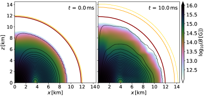
Figure 1: Meridional snapshots of the evolution of a magnetized nonrotating NS, where the RePrimAnd C2P scheme with ideal gas EOS is adopted. Black lines correspond to $A_{\phi}$ isocontours and reveal the geometry of the poloidal component of the magnetic field. The red line is the iso-density contour corresponding to 1% of the initial maximum density, whereas orange and yellow lines are the iso-density contours corresponding 100, and 5 times the artificial atmosphere density, respectively. The color scale indicates the magnetic field strength.

Our first test consists of evolving a nonrotating NS endowed with initial magnetic field confined to the NS interior. The test setup is the same as the one adopted in Cipolletta et al. (2020). To obtain initial data, we first solve the Tolman-Oppenheimer-Volkoff (TOV) equations Oppenheimer and Volkoff (1939); Tolman (1939) which describe the structure of a non-magnetized, static and spherically symmetric compact star in general relativity. As EOS, we use a polytrope $P(\rho)=K\rho^{\Gamma}$, with adiabatic index $\Gamma=2$ and polytropic constant $K=100$ (in geometric units). We consider a model with a central rest-mass density of $\rho=8.06\times 10^{14}$ g/cm³. This corresponds to a star with circumferential radius of about 12 km and a gravitational mass of about $1.4\,M_{\odot}$.

The magnetic field is then imposed onto the TOV configuration using an analytical prescription for the vector potential. The expression below corresponds to a field with dipolar structure confined inside the star:

$$\begin{split}A_{r}&=A_{\theta}=0\\ A_{\phi}&=A_{\mathrm{b}}\varpi^{2}{\rm max}\left(p-p_{\mathrm{cut}},0\right)^{n_{s}},\end{split}$$ (7)

where $A_{b}$ is a scaling factor, $\varpi$ denotes the cylindrical radius, $n_{s}=2$ represents the degree of differentiability of the field strength, and $p_{\mathrm{cut}}=0.04p_{\mathrm{max}}$ establishes the cut-off pressure, confining the magnetic field entirely inside the NS and within the region where gas pressure is $\geq 4\%$ of the maximum value $p_{\mathrm{max}}$. We chose $A_{b}$ such that the maximum magnetic field strength in the Eulerian frame is $10^{16}~{}\mathrm{G}$. While this field is rather strong compared to known magnetars, it is still not strong enough to significantly deform the star, as the magnetic energy is much smaller than the NS binding energy. We therefore leave matter distribution and spacetime metric unchanged.

We perform simulations for three different grid resolutions, i.e. low (LR), medium (MR) and high resolution (HR) using $(64)^{3}$, $(128)^{3}$ and $(256)^{3}$ grid-cells with grid spacing dx=$230.5$ m, dx=$461$ m and dx=$922$ m, respectively, in a uniform domain with $x$-, $y$- and $z$-coordinates lying in the range $[-29.5,29.5]$ km. Each simulation covers 10 ms of evolution employing the RePrimAnd primitive recovery scheme, and an atmosphere density floor set to $6.3\times 10^{6}$ g/cm³.

For the evolution, we employ two EOS implementations compatible with the initial data. One is the classical ideal gas defined by

$$P(\rho,\epsilon) =\rho\epsilon(\Gamma-1),$$ (8)

using $\Gamma=2$. The other is the hybrid gamma-law EOS defined by

$$P(\rho,\epsilon) =P_{c}(\rho)+(\epsilon-\epsilon_{c}(\rho))\rho(\Gamma_{\text{th}}-1),$$ (9)

where we use the initial data polytropic EOS for the zero-temperature curves of pressure, $P_{c}(\rho)$, and specific energy, $\epsilon_{c}(\rho)$, and further set $\Gamma_{\text{th}}=\Gamma=2$.

Evaluating the two expressions yields exactly the same EOS function $P(\rho,\epsilon)$, but there is a subtle difference regarding the definition of temperature and the validity range. When specifying an EOS as $P(\rho,\epsilon)$, there is an ambiguity about the definitions of entropy and temperature. We recall that for the classical ideal gas, the pressure and specific internal energy are proportional to the temperature, and the lower validity bound given by zero temperature is $\epsilon\geq 0$. For the hybrid EOS, the zero temperature curve is the polytrope and the lower validity bound is $\epsilon\geq\epsilon_{c}(\rho)$. The RePrimAnd C2P scheme enforces those validity ranges for ideal gas and hybrid EOS, which might introduce small differences between simulations using the two. The Noble scheme on the other hand does not enforce EOS validity ranges.

To assess the consequences, we perform simulations of the same initial data using either the ideal gas or the equivalent hybrid EOS. As long as the C2P functions correctly, we expect identical results for the Noble scheme and RePrimAnd in conjunction with the classical ideal gas EOS (assuming that the specific energy might drop below the polytrope but still remains positive). This point is relevant because not all types of EOS can be evaluated outside the physically meaningful range, most notably fully tabulated EOS. Without an EOS-agnostic policy regarding validity ranges, C2P schemes might behave differently for different types of EOS.

Fig. 1 shows snapshots of initial and final magnetic field strength and density contours, for the HR run with the RePrimAnd scheme. The low-density region at the surface is undergoing an expansion due to spurious heating, which is a typical behavior for evolution schemes near NS surfaces. In 10 ms, the magnetic field configuration also shows some variations, in particular in the outer portion of the NS (radii above $\simeq\!6$ km). We note that the simulation time span is of the order of the Alfvén timescale at this field strengths and thus field readjustments can occur, possibly triggered by the know instability of purely poloidal fields (e.g., Ciolfi et al. (2011) and refs. therein). The evolution of the normalized maximum rest-mass density $\rho_{\mathrm{max}}$ and maximum magnetic field strength $B_{\mathrm{max}}$ is reported in the top and bottom panels of Fig. 2, respectively, for all three resolutions.

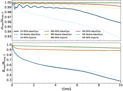
Figure 2: Evolution of normalized maximum rest-mass density (top) and magnetic field strength (bottom) for low (LR), medium (MR), and high resolution (HR) simulations, comparing also between the Noble C2P (dashed lines) scheme and the RePrimAnd (RPA) scheme, the latter either in conjunction with the ideal gas EOS (solid lines) or the hybrid EOS (dotted lines).

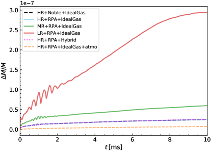
Figure 3: Relative change in total baryonic mass for the different tests with Noble and RePrimAnd schemes.

The maximum density $\rho_{\mathrm{max}}$ shows oscillations which are decaying while the system settles toward a numerical equilibrium. As we will show later, those oscillations correspond to oscillation modes expected from perturbation theory. With increasing resolution, the initial excitation amplitude decreases. In addition, $\rho_{\mathrm{max}}$ and $B_{\mathrm{max}}$ exhibit a continuous drift, which we attribute to numerical evolution errors (compare also Baiotti et al. (2005)). With increasing resolution, such a drift clearly decreases.

To assess the overall convergence behavior, we consider the time evolution of maximum density, maximum magnetic field strength, and minimum lapse function. Using the $L_{2}$ norms over time of the differences between high and medium resolution and between medium and low resolution, we find an average convergence order around 2.5 for the density, 2.7 for the magnetic field, and 3.1 for the lapse. At the finite resolutions used here, this is typical behavior for such simulations, which employ numerical schemes with different convergence orders for spacetime and magnetohydrodynamic parts.

Comparing the results obtained with the Noble scheme and the RePrimAnd scheme in conjunction with the ideal gas evolution EOS, we observe an exact match. Both schemes are equally capable to handle this test case.

Comparing between the RePrimAnd scheme with ideal gas and equivalent hybrid EOS, we find a somewhat larger drift for the latter. The only difference in the evolution is that for the hybrid EOS, the specific energy is mapped back to the value given by the polytropic cold EOS when evolution errors cause it to fall below. Hence, the correction only increases the internal energy. We conclude that on average, enforcing the validity range slightly increases the spurious heating. Enforcing the validity range might seem like a drawback, but should be weighted against consistent behavior for any type of EOS.

Since the artificial atmosphere is also handled by the C2P implementations, it is important to validate the conservation of total baryonic mass. Fig. 3 shows the total baryonic mass, comparing the different resolutions for the RePrimAnd case, the RePrimAnd and Noble schemes at high resolution, and the RePrimAnd case with ideal gas and hybrid EOS. For completeness, we compare two different measures for the mass, including and excluding the artificial atmosphere contribution. Both the Noble and RePrimAnd implementations meet the expectations for mass conservation, and agree exactly for the case of ideal gas (for all resolutions). The enforcing of validity bounds for the hybrid EOS does not have an impact on mass conservation, as expected.

In Fig. 4, we plot the power spectrum of the maximum rest-mass density evolution. As one can see, the spectra obtained with the RePrimAnd and Noble schemes are identical. Further, the spectrum shows clear peaks that are located at frequencies of the radial NS oscillation modes, predicted in Font et al. (2000) using a 2D perturbative code. The oscillations of maximum density visible in Fig. 2 thus correspond to NS oscillations excited by the deviation of initial data from equilibrium.

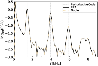
Figure 4: Fourier transform of the maximum rest-mass density evolution normalised to the amplitude of first frequency peak, for both the RePrimAnd and Noble schemes. The dash-dotted vertical lines represent the normal mode frequencies computed independently via a perturbative code as reported in Font et al. (2000).

Finally, we assess the computational costs of the two C2P implementations. Using the timing functionality available in the Einstein Toolkit, we find that both schemes use about $2.5\%$ of the total computational time. For the test at hand, the C2P is not a computational bottleneck of the Spritz code, and the computational efficiency of both schemes is similar. We note that the fraction spent in the C2P might increase significantly when using a much slower type of EOS, for example an interpolation table using temperature as one independent variable (see also the discussion in Kastaun et al. (2021)).

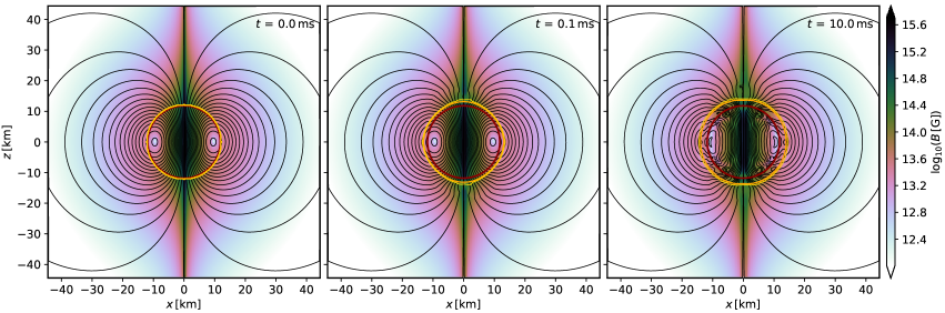
Figure 5: Results for the test case of a nonrotating NS endowed with an external dipolar magnetic field, evolved with the RePrimAnd C2P scheme and using a low artificial atmosphere density of $6.3\times 10^{5}$ g/cm³. The black lines are isocontours of the vector potential component $A_{\phi}$. Rest mass density contours in red, orange and yellow are illustrated in the same fashion as done in Fig. 1.

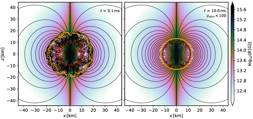
Figure 6: Results for the external dipole test obtained with the Noble C2P scheme. Left: Same as the middle panel of Fig. 5, but showing the instability developing when adopting the Noble scheme. Right: Snapshot after $10$ ms evolution with the Noble C2P scheme when using an artificial atmosphere density of $6.3\times 10^{7}$ g/cm³, enlarged by a factor 100 compared to the RePrimAnd simulation results shown in the right panel of Fig. 5.

III.2 Neutron star with extended dipolar magnetic field

A critical aspect for any primitive variable recovery scheme for MHD is the ability to handle high magnetizations in low density regimes. While the RePrimAnd scheme has proven to be robust and reliable when dealing with extremely high magnetisations in pointwise (i.e. single fluid element) tests (see Kastaun et al. (2021) for details), more delicate dynamical tests involving high magnetizations together with a nontrivial global evolution represent the next necessary step for a full validation in view of future BNS merger simulations.

Here, we simulate the same nonrotating NS model as reported in Sec. III.1, but now endowed with a dipole magnetic field also extending outside its surface. In detail, the initial magnetic field is set up employing a vector potential of the form (also used in Mösta et al. (2020))

$$\begin{split}A_{r}&=A_{\theta}=0,\\ A_{\phi}&=B_{0}\frac{r^{3}_{0}}{r^{3}+r^{3}_{0}}r\sin\theta,\end{split}$$ (10)

where $B_{0}\!=\!10^{15}$ G (corresponding to a maximum magnetic field strength of $\simeq 6.6\times 10^{15}$ G), and we assume $r_{0}=12$ km.

We perform a simulation using the RePrimAnd scheme together with the ideal gas EOS. The grid domain extends up to 44.3 km in all cartesian directions, with grid spacing of $dx\simeq 231$ m (corresponding to the high resolution introduced in the previous Section). In order to make the test more demanding, we chose a very low artificial atmosphere density of $6.3\times 10^{5}$ g/cm³.

We evolved the system up to $10$ ms without encountering any problems. Most importantly, the RePrimAnd C2P scheme worked robustly even in the low-density regions outside the NS, where the magnetic-to-fluid pressure ratio $\beta^{-1}$ reaches large values up to $\sim 10^{4}$. Fig. 5 shows three snapshots of the magnetic field strength in the meridional plane, along with vector potential and rest-mass density contours. Apart from some small drift due to normal evolution errors, the field structure remains stable.

When evolving the same configuration using the Noble scheme, the simulation develops strong instabilities after only $\simeq 0.1$ ms. These instabilities first appear shortly outside the NS surface in the polar region, where the magnetic field strength is largest. Subsequently, they spread around the rest of the star. As shown in the left panel of Fig. 6, the magnetic field in the outer layers of the NS becomes highly disordered and even the density isocontours reveal a very complex, unexpected dynamics that ultimately leads to failures in spacetime evolution. The exact mechanism behind the instability is unknown. One possible explanation is that the inaccuracies of the Noble C2P solution might be larger in the parameter space of the affected regime and then interact with the evolution scheme in an unstable manner. Since the Noble scheme depends on initial guesses from the evolution, such effects would be difficult to reproduce in standalone tests such as Siegel et al. (2018).

When the atmosphere floor density is increased by a factor of 100, the simulation performs well also with the Noble scheme, as shown in the right panel of Fig. 6. Further tests show that increasing the atmosphere density by an intermediate factor 10 is not sufficient and still leads to an early failure. We therefore attribute the failure to the magnetization, which is maximal at lowest density and hence reduced by increasing the atmosphere density.

When using the Noble scheme with 100 times larger atmosphere, the overall results (NS surface aside) are very similar to the RePrimAnd case with the original low density atmosphere. Fig. 7 compares the evolution of maximum rest-mass density $\rho_{\mathrm{max}}$ (top panel), central magnetic field strength $B_{\mathrm{c}}$ (middle panel), and total magnetic energy (bottom panel) for the two cases.

The tests clearly show that the RePrimAnd C2P scheme increases the robustness of the Spritz code when dealing with magnetic-to-fluid pressure ratios at least up to $\beta^{-1}\sim 10^{4}$, compared to the Noble scheme used previously. We stress that our study is not testing the accuracy of the numerical evolution in highly magnetized low-density regions, and point out that evolving such regions more accurately might require specialized evolution schemes incorporating the force-free approximation and/or resistive MHD. However, it is already a big advantage that the presence of such regimes is not causing a failure of the whole simulation.

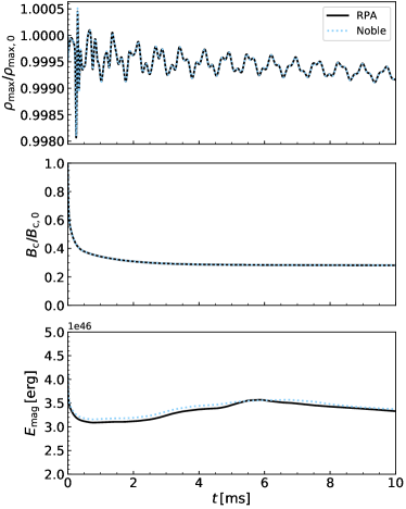
Figure 7: Evolution of normalized maximum rest-mass density (top), normalized magnetic field strength at the center (middle), and magnetic energy (bottom) for the case of a nonrotating NS endowed with extended dipolar magnetic field, evolved with the RePrimAnd C2P scheme and artificial atmosphere density of $\rho_{\mathrm{atm}}=6.3\times 10^{5}$ g/cm³ or with the Noble C2P scheme and $\rho_{\mathrm{atm}}=6.3\times 10^{7}$ g/cm³.

III.3 Rotating magnetized neutron star

Moving to a more demanding test, we now consider a uniformly rotating NS with magnetic field extending outside the star. The initial data are generated using the Hydro_RNSID module of the Einstein toolkit. Our model employs a $\Gamma=2$ polytropic EOS with $K=100$ (in units $c=G=M_{\odot}=1$), a central density $\rho_{\rm c}\simeq 6.87\times 10^{14}$ g/cm³ and a polar-to-equatorial radius ratio of 0.8744. This produces a uniformly rotating NS on the stable branch with a gravitational mass of 1.4 $M_{\odot}$, an equatorial radius of 15.65 km, and a rotation rate of 500 Hz.

We add an extended dipolar magnetic field on the NS in the same way as done in Sec. III.2. The magnetic dipole axis coincides with the rotational axis. Different to Sec. III.2, we do not add the magnetic field to the initial data, but evolve the non-magnetized initial data for 10 ms before imposing the magnetic field. The motivation for this choice is to obtain a test case that is representative for the application to binary neutron star mergers using an approach similar to, e.g., Ruiz et al. (2016), where the extended magnetic field is added to the NSs during the last orbits before merger.

After 10 ms of evolution without magnetic field, the NS is surrounded by a hot, low-density cloud of matter. Such diffuse halos are a typical effect of perturbations near the NS surface initially triggered by numerical evolution errors. This expansion of the outer layers, along with the interaction with the artificial atmosphere, also leads to strong differential rotation in the corresponding regions. For the actual test, we then evolve the magnetized system for another 10 ms. The atmosphere floor density is again set to a low value of $6.3\times 10^{5}$ g/cm³.

For this test, we also use ‘box-in-box’ mesh refinement with four refinement levels. The coarsest(finest) computational grid extends up to $\simeq 591(74)$ km in all Cartesian directions, and the finest grid spacing is $dx=461$ m, which is twice as large as the grid spacing used in the previous test. This setting gives about 26 grid points along the NS radius. The test allows us to validate the correct interplay between the implementation of the new C2P scheme in Spritz and the mesh refinement.

Fig. 8 shows the magnetic field strength on the meridional plane along with selected isocontours of rest-mass density, both at 10 ms (time at which the field is added) and 20 ms (final simulation time).

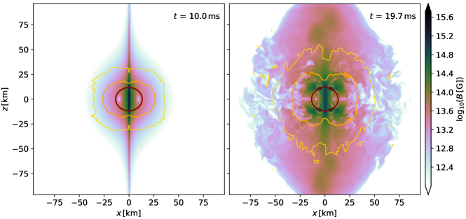
Figure 8: Meridional view of a magnetized rotating NS, evolved using the RePrimAnd C2P scheme. Color scale indicates the magnetic field strength and the iso-density contours are the same as in Fig. 1. Left panel shows the time at which an extended dipolar magnetic field is imposed (10 ms), while the right panel shows the system towards the end of the simulation.

Right after the field is imposed, it starts to get distorted by the motion of the low density material surrounding the NS bulk. Differential rotation leads to magnetic winding and the appearance of a toroidal component. The resulting magnetic pressure gradients contribute to the expansion of the outer layers of the NS and of the surrounding matter.

In Fig. 9, we plot the field line structure close to the star towards the end of the simulation, using the visualization method developed in Kawamura et al. (2016) but focusing more on the regions near the NS and rotation axis.

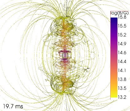
Figure 9: Three dimensional magnetic field structure of the system shown in right panel of Fig. 8. A sphere of radius 10 km is added in the center to give a spatial scale reference.

Along the spin axis and up to about 100 km from the center, we observe the twisting of magnetic field lines. At large distances, within the artificial atmosphere, the original dipolar structure remains frozen (see Sec. II). We stress that a proper treatment of those outer regions would require a force-free evolution, which is not currently implemented in Spritz.

During the whole simulation, the RePrimAnd C2P scheme experienced no difficulties while handling the high magnetizations present in the low density regions, where the magnetic-to-fluid pressure ratio reaches $\sim\!10^{4}$.

III.4 Rotating magnetized neutron star collapse

Our next test case consists of evolving the collapse of a magnetized differentially rotating hypermassive NS to a BH. Even though the gauge conditions avoid the physical singularity, the center of BHs is challenging for numerical evolution schemes. The purpose of the test is not just to demonstrate the robustness of the C2P scheme under the conditions encountered during BH formation, but also to validate that the interplay between our policy for corrections and the time evolution scheme results in a stable evolution of a BH with matter. As described in Sec. II, we evolve the BH interior without excision, but employ a C2P policy near the center that effectively limits the velocity and specific energy.

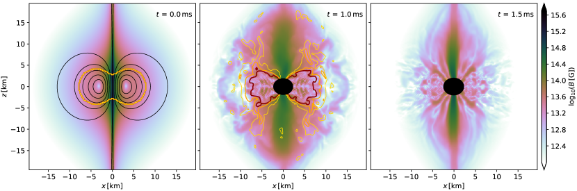
Figure 10: Meridional snapshots of magnetic field strength for the magnetized rotating NS collapse simulation, evolved using the RePrimAnd C2P scheme. The iso-density contours in red, orange, and yellow correspond to 5, 3 and 1.5 times the artificial atmosphere density, respectively. The left panel, referring to the initial setup, shows also the magnetic field geometry as $A_{\phi}$ isocontours (black). The middle and right panels refer to 1 and 1.5 ms of evolution, respectively. The $A_{\phi}$ isocontours are not shown in the last two panels as their disordered structure overcrowds the regions of interest we want to show. The black area marks the apparent horizon of the BH.

For this test, we adopt the dynamically unstable axisymmetric model A2 of Giacomazzo et al. (2011), which consists of a hypermassive NS close to collapse. It employs a polytropic EOS with $\Gamma=2$ and $K=100$. The model has a gravitational mass of $M\simeq 2.228\,M_{\odot}$ and a central rest-mass density of $\rho_{\rm c}\simeq 1.892\times 10^{15}$ g/cm³. The model follows the “j-constant law” of differential rotation, with differential rotation parameter $\hat{A}=1$ (see Giacomazzo et al. (2011) for details) and central angular velocity $\Omega_{\rm c}\simeq 44\,\mathrm{Rad}/\mathrm{ms}$. The resulting ratio of the polar to the equatorial coordinate radii is $r_{\rm p}/r_{\rm e}=0.33$.

The non-magnetized model is constructed using the Hydro_RNSID module of the Einstein Toolkit. On top of this initial configuration, we add an extended dipolar magnetic field in the same fashion as done in Sec. III.2, with $B_{0}=10^{15}$ G. However, in this case we choose $r_{0}=4$ km.

The computational grid setup is the one described in Sec. III.3, supplemented with an additional inner refinement level that has a grid spacing of $dx\simeq 230.5$ m and which extends up to $[-37,+37]$ km in all three directions. The system is evolved with Spritz, employing the RePrimAnd C2P scheme together with an ideal gas EOS with $\Gamma=2$. The atmosphere floor density is again set to $6.3\times 10^{5}$ g/cm³.

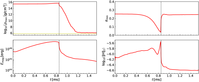
Figure 11: Evolution of maximum rest-mass density normalized to the initial value (top-left), total magnetic energy (bottom-left), minimum of lapse (top-right), and L2 norm of the Hamiltonian constraint (bottom-right). Once the BH is formed, the interior of the apparent horizon is excluded for the computation of these quantities. The vertical black (dashed) line in all panels marks the time at which the apparent horizon is found in the simulation, while the horizontal yellow line in the top-left panel represents the floor density.

We evolve the system for around 1.5 ms, which is sufficient to capture the collapse of the hypermassive star and the formation of the BH. Prior to collapse (occurring at $\simeq\!0.84$ ms), the outer layers of the NS tend to expand due to spurious heating, while the central core is slightly contracting. The initially ordered and purely poloidal magnetic field is wound up by differential rotation, which creates a toroidal component and amplifies the overall field strength. At the same time, the field becomes more disordered within the expanding outer layers of the NS, due to the irregular fluid motion. After BH formation, matter is rapidly absorbed and the magnetic field is also dragged along by the in-falling material. Fig. 10 illustrates the magnetic field strength at the initial, intermediate, and final times of the simulation. Throughout the simulation, we do not find any significant artifacts in magnetic field at the refinement level jumps.

The above dynamics is reflected in the time evolution of maximum rest-mass density $\rho_{\rm max}$, total magnetic energy $E_{\rm mag}$, minimum lapse $\alpha_{\rm min}$, and $L_{2}$-norm of the Hamiltonian constraint $H$, which are shown in Fig. 11. Note that once the BH has formed, the interior of the apparent horizon is excluded from those measures.

We conclude that the RePrimAnd scheme can be used for scenarios involving BH formation, most notably BNS and NS-BH mergers. Moreover, the robustness and flexibility in applying corrections allows to evolve BHs in GRMHD schemes without applying any form of excision in the center of the BH.

III.5 Fishbone-Moncrief BH-accretion disk

For our final 3D test of the RePrimAnd scheme, we simulate a magnetized accretion disk surrounding a Kerr BH, based on the equilibrium torus solutions proposed by Fishbone and Moncrief (1976). A BH-disk system is one of the typical outcomes of BNS/NS-BH mergers (e.g., Paschalidis et al. (2015); Ciolfi et al. (2017); Foucart et al. (2019); Shibata and Hotokezaka (2019); Bernuzzi et al. (2020); Bernuzzi (2020); Ruiz et al. (2020); Kastaun and Ohme (2021)) and model investigations of such systems probe the underlying mechanisms that govern the dynamics of the plasma accretion, post-merger disk winds that contribute to kilonova emission, as well as launching of relativistic jets. Such a system has also been widely used as a standard test case for different evolution codes and schemes Gammie et al. (2003); Noble et al. (2006, 2009); Porth et al. (2017); Janiuk et al. (2018); Ripperda et al. (2019); Murguia-Berthier et al. (2021). In our case, evolving such a configuration allows another crucial check on the robustness of the RePrimAnd scheme when dealing with accretion onto a BH and MHD turbulence.

The initial data for spacetime and hydrodynamic variables is built using the FishboneMoncriefID thorn of the Einstein Toolkit Löffler et al. (2012); Zilhão and Löffler (2013), which has been adapted to work with Spritz . The public version of thorn was also used, e.g., to setup the IllinoisGRMHD Etienne et al. (2015) simulations in the code comparison reported in Porth et al. (2019). For the initial data, we use a polytropic EOS with $\Gamma=4/3$ and $K\simeq 0.156$, while for the evolution we use an ideal gas EOS with $\Gamma=4/3$. We set the initial Kerr BH mass to $2.7\,M_{\odot}$ and its dimensionless spin parameter to $a=0.9$. This results in an equatorial BH horizon radius of about 7.8 km in simulation coordinates. The inner edge of the torus is located at a coordinate radius $r_{in}\approx 24\,$km, and the maximum density (9.76$\times 10^{11}$ g/cm³) is reached at coordinate radius $r_{max}\approx 48\,$km. This matter configuration is then complemented by a purely poloidal magnetic field confined inside the torus, using expression Eq. (7), and choosing an initial maximum magnetic field strength of $10^{14}$ G, which corresponds to an initial magnetic-to-fluid pressure ratio $\beta^{-1}$ of about $2\times 10^{-4}$. As before, the atmosphere floor density is set to $6.3\times 10^{5}$ g/cm³ for the entire domain.

For this test, we use a fixed spacetime metric that is not evolved in time. The metric we use has a coordinate singularity at the origin. Nevertheless, we evolve the magnetohydrodynamic equations in the full domain. In order to avoid singular values, we place the numerical grid such that the origin is located at the corners of the adjacent cells on the finest refinement level, and never at a cell center. Still, the large gradients that spacetime-related variables exhibit near the origin pose a challenging test for the robustness of the code.

We employ fixed ‘box-in-box’ mesh refinement, using a computational grid hierarchy with five cubical refinement levels. The coarsest level extends up to $528\,$km and the finest one up to $33\,$km, with a resolution of $\sim 531.6$ m. For the chosen grid hierarchy, some mesh refinement boundaries are crossing the disk. This could be avoided in a production setting, but as test case facilitates the observation of potential artifacts.

Related to the potentially problematic mesh refinement boundaries and BH center, we test several evolution options. One is to employ the algebraic gauge condition Etienne et al. (2012, 2010) for the vector potential, but without using any artificial numerical dissipation. Next, we use the generalized Lorenz gauge (see Eq. (29) of Cipolletta et al. (2020)) still without dissipation. Finally, we use the generalized Lorenz gauge while applying Kreiss-Oliger dissipation Kreiss and Oliger (1973) to the evolved vector and scalar potentials. In particular, we use the Dissipation module of the Einstein Toolkit, with dissipation order $p=5$ and dissipation strength parameter $\epsilon_{\text{diss}}=0.1$, which is a typical value used in other works (see, for e.g., Kawamura et al. (2016); Ciolfi et al. (2017, 2019)).

For the test case at hand, the use of the algebraic gauge leads to numerical instabilities at the mesh refinement boundaries inside the disk. This seems related solely to the evolution, whereas the C2P algorithm was not causing any problems. As an additional cross-check, we verified that the same behavior arises when using the Noble C2P scheme. The evolution using Lorenz gauge without dissipation shows high-frequency noise at the refinement boundaries, as well as numerical instabilities near the origin . Again, the C2P algorithm was not causing problems.

When using the Lorenz gauge with dissipation, we obtain a stable evolution without artifacts near the mesh refinement boundaries. We evolve this case for about 50 ms. The rest-mass density distribution at initial and final time is shown in Fig. 12.

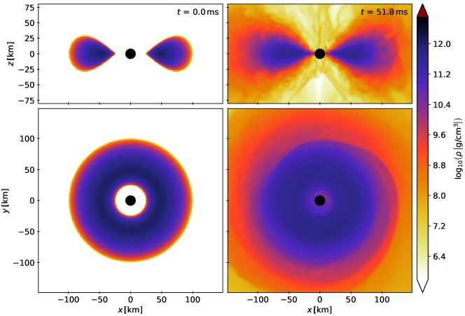
Figure 12: Initial and final time snapshots of the rest-mass density in the meridional (top-row) and equatorial (bottom-row) planes for the magnetized Fishbone-Moncrief BH-accretion disk test. The apparent horizon is depicted in black.

Within the first few ms, disk matter starts to fall into the BH, in part channeled along the BH spin axis, while the inner edge of the disk moves closer and closer to the horizon on the equatorial plane. At the same time, the outer layers of the disk begin to expand and the initial sharp outer edge of the disk is lost in favor of a layer of low density material gradually spreading up to larger and larger distances. At the end of the simulation ($\sim\!50$ ms), after the initial transient phase, it looks as if the system is starting to adjust towards a quasi-stationary configuration. The latter condition would however be fully achieved only via longer simulations, as reported in the literature (see, e.g., Porth et al. (2019)).

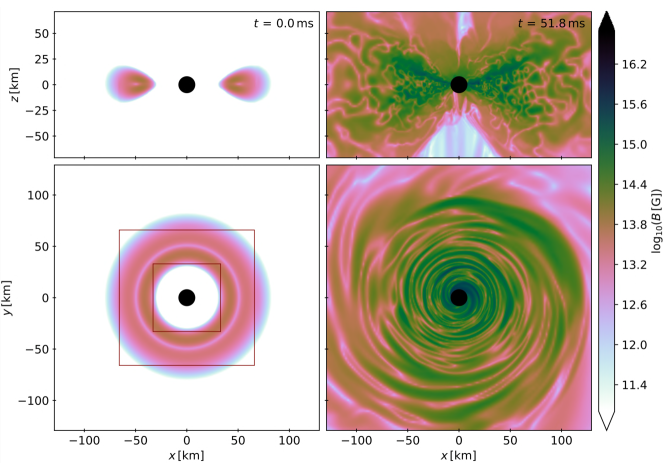
Figure 13: Initial and final time snapshots of the magnetic field strength within the meridional (top-row) and equatorial (bottom-row) planes, for the magnetized Fishbone-Moncrief BH-accretion disk test. The apparent horizon is depicted in black. In the lower left panel, we also highlight the mesh-refinement boundaries (red).

Fig. 13 illustrates the magnetic field strength at the initial and final time frames. For comparison, we draw the locations of the mesh refinement boundaries in one panel, illustrating that there are no significant artifacts present until the end of simulation. During the evolution, magnetic fields get dragged along with the fluid into the BH horizon as shown in the right-panels of Fig. 13. Moreover, the magnetic field within the disk undergoes a strong amplification, particularly in the toroidal component, induced by the differential rotation and shear in the disk. The maximum magnetic field strength grows by about two orders of magnitude in 50 ms, aided by magnetic winding, and potentially the development of the magneto-rotational instability (MRI). Using $\lambda_{\rm MRI}\approx(2\pi/\Omega)\times B/\sqrt{4\pi\rho}$ as an estimate for the wavelength of the fastest growing mode, we find that at 50 ms it is resolved by 10–100 grid points in most of the disk, with local growth timescales of order 1–10 ms. Overall, magnetic energy grows by around three orders of magnitude as shown in Fig. 14, and $\beta^{-1}$ increases more than the maximum field strength, reaching values up to 100. The reason is that the regions of low density above and below the disk become increasingly permeated by strong fields.

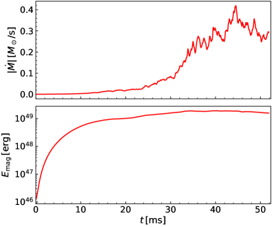
Figure 14: Time evolution of the mass accretion rate (top-panel) and total magnetic energy (bottom-panel) for the magnetized Fishbone-Moncrief BH-accretion disk test.

The top panel of Fig. 14 shows the mass accretion rate, computed from the mass flux penetrating the horizon (in detail, we consider the mass flow rate through a spherical surface of radius $\sim\!7.83$ km that is slightly larger than the BH). We find that after $10$–$12$ ms, the accretion rate starts to rapidly grow and the increase continues up to a maximum reached around 45 ms. Towards the end of the simulation, we observe first hints of saturation and what appears to be the beginning of a decreasing trend. We note that on longer timescales, a jet might form as well. The current test should not be regarded as representative for this scenario, since it would involve magnetizations, temperatures, and velocities that exceed those reached here.

For comparison, we repeated the test with the same setup, but employing the Noble C2P implementation of the Spritz code. We observed instabilities similarly to the results shown in Sec. III.2, as well as outright C2P failures, which occur within $1\,\mathrm{m}\mathrm{s}$. Those problems occur in a region extending outside the horizon, including the inner edge of the disk. When increasing the atmosphere density to 10 (100) times the one used for RePrimAnd test, similar failures occur within $5(11)\,\mathrm{m}\mathrm{s}$.

In conclusion, our RePrimAnd scheme implementation functions well in the regimes encountered within the first 50 ms of evolution of the chosen magnetized Fishbone-Moncrief BH-accretion disk setup, for a floor density as low as $6.3\times 10^{5}$ g/cm³ and a (rather low) finest resolution of $\sim\!530$ m. It is more reliable than the old C2P implementation, which failed such a test. The RePrimAnd scheme is also functioning robustly in the presence of numerical instabilities in the evolution itself, caused by other effects such as coordinate singularities. The physical setup in this test is representative for science runs involving long-term evolution of post-merger accretion disks around BHs before (or without) jet formation.

IV Conclusions and Outlook

In this work, we implement our new primitive variable recovery scheme RePrimAnd Kastaun et al. (2021) in the GRMHD code Spritz. We perform a number of demanding 3D GRMHD tests representative for astrophysical scenarios, including binary neutron star mergers and BH formation. In addition, we carried out various 1D shock tube tests with known solution up to high magnetization. Those tests validate the correctness of the implementation as well as the stability of the interplay of the evolution scheme with the recovery scheme. We also discuss important technical details regarding the treatment of invalid states, validity bounds of the EOS, and the evolution inside BHs without use of excision.

When evolving a TOV configuration with magnetic field confined entirely inside the star, the field evolution is well-behaved and our resolution study shows equivalent results for test cases using the RePrimAnd scheme and the commonly used scheme of Noble et al. Noble et al. (2006), establishing an important consistency check.

Next, we consider the same TOV configuration, but with an initial dipolar magnetic field extending also outside the NS surface. This test shows the ability of the RePrimAnd scheme to handle magnetized, low density environments with magnetic-to-fluid pressure ratios reaching $\sim\!10^{4}$. In particular, we find that the RePrimAnd scheme performs well for the extremely low artificial atmosphere density of $6.3\times 10^{5}$ g/cm³ used in this test. In contrast, we find that the Noble scheme fails unless the floor density is increased by at least two orders of magnitude.

In another test, we start from a non-magnetized uniformly rotating NS and add the same extended dipolar field after 10 ms, then evolve the system for another 10 ms. At the time the magnetic field is added, the outermost layers of the star have expanded and are no longer uniformly rotating. Such a differential rotation winds up the field, generating a growing toroidal component, while at larger distances the dipolar field structure remains essentially unaffected. The RePrimAnd scheme shows again efficient handling of magnetic-to-fluid pressure ratios as high as $\sim\!10^{4}$. Additionally, this test case ascertains correct behavior when employing mesh-refinement.

The crucial test case of a magnetized differentially rotating NS collapsing to a rotating BH successfully proves the robust performance of the scheme also in highly dynamical conditions and for highly magnetized environments around BHs. Moreover, it shows that the scheme is not causing problems when evolving the interior of the BH without excision. This test is fundamental for NS-NS/NS-BH merger simulations that involve a BH merger remnant surrounded by a magnetized disk, and in particular for studies related to development of magnetically driven relativistic jets by such BH-disk systems.

As our final 3D test, we simulate an accreting BH-disk system, starting from a Fishbone-Moncrief equilibrium solution where a poloidal magnetic field was added inside the disk. The system is evolved for 50 ms, long enough to show the first signs of saturation in the growth of the accretion rate. We also observe strong magnetic field amplification, most likely caused by a mixture of magnetic winding and the development of the magneto-rotational instability. As a side-effect, this setup also investigates the interplay between numerical evolution scheme and mesh-refinement with refinement boundaries intersecting the disk. We find that artifacts can be avoided by using the generalized Lorenz gauge together with Kreiss-Oliger dissipation. As in the previous test, we evolve the BH interior without excision. Instead, we exploit the flexibility offered be the RePrimAnd scheme regarding the handling of extreme or invalid states, by employing different policies inside and outside the BH. Also in this test, the new primitive recovery scheme is not causing any problems.

Building on the proven robustness of the RePrimAnd scheme, we are currently working on providing support for using the new scheme in Spritz also with a fully-tabulated, composition and temperature dependent EOS. In the near future, we plan to use this additional upgrade of the scheme to perform magnetized BNS or NS-BH merger simulations as well as long-term BH-disk simulations with microphysical EOS and including an approximate treatment of neutrino radiation.

Appendix A Shock tube tests

In the following, we describe the results of basic 1D shock tube tests. Since the exact solution is known for those tests, they are ideal to validate the basic correctness of the full evolution code. Our focus is on the robustness of the recovery schemes as used in the evolution code. For a general discussion of the accuracy of the numerical evolution scheme in shock tube problems, we refer to Cipolletta et al. (2020) and the references therein. Here, we compare results obtained both using the Noble recovery scheme and the new RePrimAnd scheme.

First, we repeat a series of tests known as Balsara problems 1–5 Balsara (2001), which have already been carried out with older Spritz code versions in Cipolletta et al. (2020). These tests use an ideal gas EOS. We set the artificial atmosphere to much lower values than encountered in the simulations. When using the RePrimAnd recovery, we also effectively disable the optional corrections (using a low value for $\rho_{\rm strict}$). Balsara tests 1 to 4 are evolved until a time $t=0.4$ and Balsara 5 up to $t=0.55$ using 1600 grid points in the domain extending from -0.5 to 0.5 along x-direction.

We find no significant differences between results with Noble and RePrimAnd schemes and neither scheme develops problems. The solution matches the exact solution (obtained via the code presented in Giacomazzo and Rezzolla (2006)) as well as expected for such tests (see Cipolletta et al. (2020)). We note that the Balsara tests only reach a magnetization of $\beta^{-1}{\approx}500$.

To test the code in a more demanding regime with higher magnetization, we created two new shock tube configurations labeled A and B in the following. The parameters are reported in Table 1. Both use an ideal gas EOS with $\Gamma=5/3$ and are evolved up to time $t=0.4$ using 1600 grid points with the domain extension $[-0.5,0.5]$ along x-direction. Configuration A reaches a magnetization $\beta^{-1}=1.6\times 10^{4}$, and configuration B an even higher value $10^{5}$.

The results for the two recovery schemes are shown in Figure 15. For test A, the plots show exact matches between the two schemes, and typical deviations from the exact solution. In contrast, we find significant differences between the schemes for test B. The reason is that the Noble scheme occasionally fails to converge and then falls back to the use of a polytropic EOS instead of the correct ideal gas EOS. In some instances, even the fallback approximation fails to converge, and non-converged results are used. The RePrimAnd scheme did not experience any problems with the stronger magnetization of this test. Correspondingly, the solution is closer to the exact one in the affected regime.

Test:	A		B
	L	R	L	R
$\rho$	0.1	0.1	0.1	0.1
$p$	10.0	0.1	10.0	0.1
$v^{x}$	0.01	-0.01	0.01	-0.01
$v^{y}$	0.0	0.0	0.0	0.0
$v^{z}$	0.0	0.0	0.0	0.0
$B^{x}$	0.0	0.0	0.0	0.0
$B^{y}$	40.0	40.0	100.0	100.0
$B^{z}$	40.0	40.0	100.0	100.0

Table 1: Parameters for shock tube tests A and B. Columns L and R refer to left and right states, and the shock propagates along the $x$-axis.

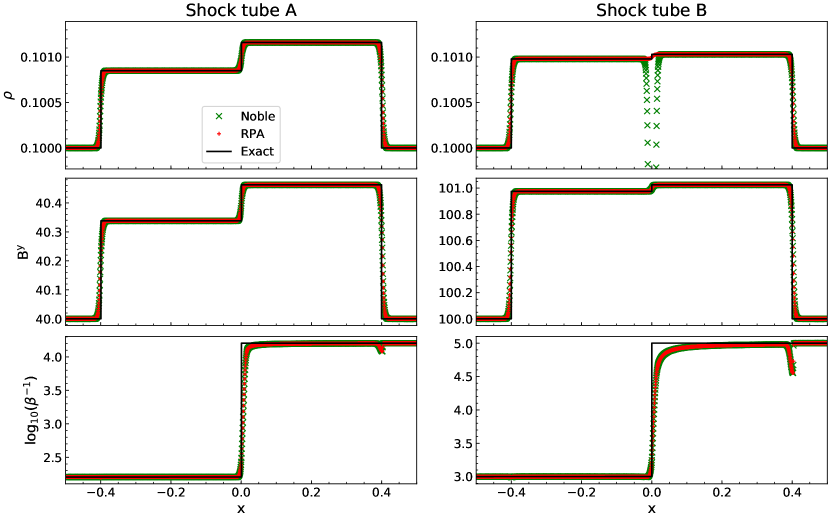
Figure 15: Shock profiles at time $t=0.4$ for test cases A and B from Table 1, evolved while using the RePrimAnd and Noble C2P schemes, in comparison to the exact solution computed using the code of Giacomazzo and Rezzolla (2006).

References

- Abbott et al. (2017a) B. P. Abbott, R. Abbott, T. D. Abbott, F. Acernese, K. Ackley, C. Adams, T. Adams, P. Addesso, R. X. Adhikari, V. B. Adya, and et al., Phys. Rev. Lett. 119, 161101 (2017a), arXiv:1710.05832 [gr-qc] .
- Abbott et al. (2017b) B. P. Abbott, R. Abbott, T. D. Abbott, F. Acernese, K. Ackley, C. Adams, T. Adams, P. Addesso, R. X. Adhikari, V. B. Adya, and et al., Astrophys. J. Lett. 848, L13 (2017b), arXiv:1710.05834 [astro-ph.HE] .
- Abbott et al. (2017c) B. P. Abbott, R. Abbott, T. D. Abbott, F. Acernese, K. Ackley, C. Adams, T. Adams, P. Addesso, R. X. Adhikari, V. B. Adya, and et al., Astrophys. J. Lett. 848, L12 (2017c), arXiv:1710.05833 [astro-ph.HE] .
- Lazzati et al. (2018) D. Lazzati, R. Perna, B. J. Morsony, D. Lopez-Camara, M. Cantiello, R. Ciolfi, B. Giacomazzo, and J. C. Workman, Phys. Rev. Lett. 120, 241103 (2018), arXiv:1712.03237 [astro-ph.HE] .
- Mooley et al. (2018) K. P. Mooley, A. T. Deller, O. Gottlieb, E. Nakar, G. Hallinan, S. Bourke, D. A. Frail, A. Horesh, A. Corsi, and K. Hotokezaka, Nature 561, 355 (2018), arXiv:1806.09693 [astro-ph.HE] .
- Ghirlanda et al. (2019) G. Ghirlanda, O. S. Salafia, Z. Paragi, M. Giroletti, J. Yang, B. Marcote, J. Blanchard, I. Agudo, T. An, M. G. Bernardini, and et al., Science 363, 968 (2019), arXiv:1808.00469 [astro-ph.HE] .
- Kasen et al. (2017) D. Kasen, B. Metzger, J. Barnes, E. Quataert, and E. Ramirez-Ruiz, Nature 551, 80 (2017), arXiv:1710.05463 [astro-ph.HE] .
- Pian et al. (2017) E. Pian, P. D’Avanzo, S. Benetti, M. Branchesi, E. Brocato, S. Campana, E. Cappellaro, S. Covino, V. D’Elia, J. P. U. Fynbo, and et al., Nature 551, 67 (2017), arXiv:1710.05858 [astro-ph.HE] .
- Abbott et al. (2019) B. P. Abbott, R. Abbott, T. D. Abbott, F. Acernese, K. Ackley, C. Adams, T. Adams, P. Addesso, R. X. Adhikari, V. B. Adya, and et al., Phys. Rev. X 9, 011001 (2019), arXiv:1805.11579 [gr-qc] .
- Abbott et al. (2017d) B. P. Abbott, R. Abbott, T. D. Abbott, F. Acernese, K. Ackley, C. Adams, T. Adams, P. Addesso, R. X. Adhikari, V. B. Adya, and et al., Nature 551, 85 (2017d), arXiv:1710.05835 .
- Abbott et al. (2020) B. P. Abbott et al., Class. Quantum Grav. 37, 045006 (2020).
- Ciolfi (2020a) R. Ciolfi, Front. Astron. Sp. Sci. 7, 27 (2020a), arXiv:2005.02964 [astro-ph.HE] .
- Ciolfi (2020b) R. Ciolfi, Gen. Rel. Grav. 52, 59 (2020b), arXiv:2003.07572 [astro-ph.HE] .
- Ruiz et al. (2021) M. Ruiz, S. L. Shapiro, and A. Tsokaros, Frontiers in Astronomy and Space Sciences 8, 39 (2021).
- Palenzuela et al. (2015) C. Palenzuela, S. L. Liebling, D. Neilsen, L. Lehner, O. L. Caballero, E. O’Connor, and M. Anderson, Phys. Rev. D 92, 044045 (2015), arXiv:1505.01607 [gr-qc] .
- Paschalidis et al. (2015) V. Paschalidis, M. Ruiz, and S. L. Shapiro, The Astrophysical Journal Letters 806, L14 (2015).
- Kawamura et al. (2016) T. Kawamura, B. Giacomazzo, W. Kastaun, R. Ciolfi, A. Endrizzi, L. Baiotti, and R. Perna, Phys. Rev. D 94, 064012 (2016).
- Ciolfi et al. (2017) R. Ciolfi, W. Kastaun, B. Giacomazzo, A. Endrizzi, D. M. Siegel, and R. Perna, Phys. Rev. D 95, 063016 (2017), arXiv:1701.08738 [astro-ph.HE] .
- Most et al. (2019) E. R. Most, L. J. Papenfort, and L. Rezzolla, Mon. Not. R. Astron. Soc. 490, 3588 (2019), arXiv:1907.10328 [astro-ph.HE] .
- Ruiz et al. (2019) M. Ruiz, A. Tsokaros, V. Paschalidis, and S. L. Shapiro, Phys. Rev. D 99, 084032 (2019), arXiv:1902.08636 [astro-ph.HE] .
- Mösta et al. (2020) P. Mösta, D. Radice, R. Haas, E. Schnetter, and S. Bernuzzi, Astrophys. J. Lett. 901, L37 (2020), arXiv:2003.06043 [astro-ph.HE] .
- Ruiz et al. (2020) M. Ruiz, V. Paschalidis, A. Tsokaros, and S. L. Shapiro, Phys. Rev. D 102, 124077 (2020), arXiv:2011.08863 [astro-ph.HE] .
- East et al. (2021) W. E. East, L. Lehner, S. L. Liebling, and C. Palenzuela, arXiv preprint arXiv:2101.12214 (2021).
- Most et al. (2021) E. R. Most, L. J. Papenfort, S. D. Tootle, and L. Rezzolla, Monthly Notices of the Royal Astronomical Society 506, 3511 (2021), https://academic.oup.com/mnras/article-pdf/506/3/3511/39354872/stab1824.pdf .
- Giacomazzo et al. (2020) B. Giacomazzo, F. Cipolletta, J. Kalinani, R. Ciolfi, L. Sala, B. Giudici, and E. Giangrandi, “The spritz code,” (2020).
- Cipolletta et al. (2020) F. Cipolletta, J. V. Kalinani, B. Giacomazzo, and R. Ciolfi, Class. Quantum Grav. 37, 135010 (2020), arXiv:1912.04794 [astro-ph.HE] .
- Löffler et al. (2012) F. Löffler, J. Faber, E. Bentivegna, T. Bode, P. Diener, R. Haas, I. Hinder, B. C. Mundim, C. D. Ott, E. Schnetter, and et al., Class. and Quantum Grav. 29, 115001 (2012), arXiv:1111.3344 [gr-qc] .
- Zilhão and Löffler (2013) M. Zilhão and F. Löffler, Int. J. Mod. Phys. A 28, 1340014-126 (2013), arXiv:1305.5299 [gr-qc] .
- Zachariah et al. (2021) E. Zachariah, B. Steven R., D. Peter, G. William E., G.-L. Miguel, H. Roland, K. Atul, A. Miguel, A. Daniela, A. Gabrielle, A. Marcus, B.-H. Maria, B. Luca, B. Werner, B. Eloisa, B. Sebastiano, B. Tanja, B. Gabriele, B. Brockton, B. Bernd, C. Manuela, C. Federico, C. Giovanni, C. Samuel, D. P. Roberto, D. Harry, D. Rion, D. Nils, E. Matthew, E. K. Yaakoub, F. Joshua, F. Toni, F. Joachim, G. Bruno, G. Tom, G. Carsten, H. Ian, H. Scott, H. Ian, H. E. A., H. Sascha, I. Sai, J. Daniel, K. Thorsten, K. Andrew, K. Michael, L. Pablo, L. Gerd, L. Frank, M. Joan, M. Lars, M. Andre, M. M. Jonah, M. Mark, M. Philipp, M. Pedro, M. Bruno, N. Andrea, C. N. Scott, O. Christian, P. Ravi, P. Denis, R. David, R. Thomas, R. Christian, R. Luciano, R. David, R. Matei, S. Lorenzo, A. S. Jascha, S. Erik, S. Bernard, S. Ed, S. Eric, S. John, S. Ken, S. Ulrich, S. Nikolaos, S. Wai-Mo, S. Bela, T. Ryoji, T. Michael, T. Jonathan, T. Malcolm, T. Aaryn, W. Paul, W. Mew-Bing, W. Barry, W. Leonardo, W. Helvi, Z. Miguel, Z. Burkhard, and Z. Yosef, “The einstein toolkit,” (2021).
- Cipolletta et al. (2021) F. Cipolletta, J. V. Kalinani, E. Giangrandi, B. Giacomazzo, R. Ciolfi, L. Sala, and B. Giudici, Class. Quant. Grav. 38, 085021 (2021), arXiv:2012.10174 [astro-ph.HE] .
- O’Connor and Ott (2010) E. O’Connor and C. D. Ott, Class. and Quantum Grav. 27, 114103 (2010), arXiv:0912.2393 [astro-ph.HE] .
- Ott et al. (2013) C. D. Ott, E. Abdikamalov, P. Mösta, R. Haas, S. Drasco, E. P. O’Connor, C. Reisswig, C. A. Meakin, and E. Schnetter, Astrophys. J. 768, 115 (2013), arXiv:1210.6674 [astro-ph.HE] .
- Siegel et al. (2018) D. M. Siegel, P. Mösta, D. Desai, and S. Wu, Astrophys. J. 859, 71 (2018), arXiv:1712.07538 [astro-ph.HE] .
- Kastaun et al. (2021) W. Kastaun, J. V. Kalinani, and R. Ciolfi, Phys. Rev. D 103, 023018 (2021), arXiv:2005.01821 [gr-qc] .
- Kastaun (2020) W. Kastaun, “Reprimand: Version 1.1,” (2020).
- Aguilera-Miret et al. (2020) R. Aguilera-Miret, D. Viganò, F. Carrasco, B. Miñano, and C. Palenzuela, Phys. Rev. D 102, 103006 (2020), arXiv:2009.06669 [gr-qc] .
- Noble et al. (2006) S. C. Noble, C. F. Gammie, J. C. McKinney, and L. Del Zanna, Astrophys. J. 641, 626 (2006), arXiv:astro-ph/0512420 [astro-ph] .
- Palenzuela et al. (2009) C. Palenzuela, L. Lehner, O. Reula, and L. Rezzolla, Monthly Notices of the Royal Astronomical Society 394, 1727 (2009).
- Dionysopoulou et al. (2013) K. Dionysopoulou, D. Alic, C. Palenzuela, L. Rezzolla, and B. Giacomazzo, Phys. Rev. D 88, 044020 (2013), arXiv:1208.3487 [gr-qc] .
- Ripperda et al. (2019) B. Ripperda, F. Bacchini, O. Porth, E. R. Most, H. Olivares, A. Nathanail, L. Rezzolla, J. Teunissen, and R. Keppens, The Astrophysical Journal Supplement Series 244, 10 (2019).
- Wright and Hawke (2020) A. J. Wright and I. Hawke, Monthly Notices of the Royal Astronomical Society 491, 5510 (2020), arXiv:1906.03150 [physics.plasm-ph] .
- Galeazzi et al. (2013) F. Galeazzi, W. Kastaun, L. Rezzolla, and J. A. Font, Phys. Rev. D 88, 064009 (2013), arXiv:1306.4953 [gr-qc] .
- Kastaun and Galeazzi (2015) W. Kastaun and F. Galeazzi, Phys. Rev. D 91, 064027 (2015).
- Kastaun et al. (2016) W. Kastaun, R. Ciolfi, and B. Giacomazzo, Phys. Rev. D 94, 044060 (2016), arXiv:1607.02186 [astro-ph.HE] .
- Kreiss and Oliger (1973) H.-O. Kreiss and J. Oliger, Methods for the approximate solution of time dependent problems, 10 (International Council of Scientific Unions, World Meteorological Organization, 1973).
- Oppenheimer and Volkoff (1939) J. R. Oppenheimer and G. M. Volkoff, Phys. Rev. 55, 374 (1939).
- Tolman (1939) R. C. Tolman, Phys. Rev. 55, 364 (1939).
- Ciolfi et al. (2011) R. Ciolfi, S. K. Lander, G. M. Manca, and L. Rezzolla, Astrophys. J. Lett. 736, L6 (2011), arXiv:1105.3971 [gr-qc] .
- Baiotti et al. (2005) L. Baiotti, I. Hawke, P. J. Montero, F. Löffler, L. Rezzolla, N. Stergioulas, J. A. Font, and E. Seidel, Phys. Rev. D 71, 024035 (2005), arXiv:gr-qc/0403029 [gr-qc] .
- Font et al. (2000) J. A. Font, N. Stergioulas, and K. D. Kokkotas, Mon. Not. R. Astron. Soc. 313, 678 (2000), arXiv:gr-qc/9908010 [gr-qc] .
- Ruiz et al. (2016) M. Ruiz, R. N. Lang, V. Paschalidis, and S. L. Shapiro, Astrophys. J. Lett. 824, L6 (2016), arXiv:1604.02455 [astro-ph.HE] .
- Kiuchi et al. (2012) K. Kiuchi, K. Kyutoku, and M. Shibata, Phys. Rev. D 86, 064008 (2012), arXiv:1207.6444 [astro-ph.HE] .
- Giacomazzo et al. (2011) B. Giacomazzo, L. Rezzolla, and N. Stergioulas, Phys. Rev. D 84, 024022 (2011).
- Fishbone and Moncrief (1976) L. G. Fishbone and V. Moncrief, The Astrophysical Journal 207, 962 (1976).
- Foucart et al. (2019) F. Foucart, M. D. Duez, L. E. Kidder, S. M. Nissanke, H. P. Pfeiffer, and M. A. Scheel, Phys. Rev. D 99, 103025 (2019), arXiv:1903.09166 [astro-ph.HE] .
- Shibata and Hotokezaka (2019) M. Shibata and K. Hotokezaka, Annual Review of Nuclear and Particle Science 69, 41 (2019), arXiv:1908.02350 [astro-ph.HE] .
- Bernuzzi et al. (2020) S. Bernuzzi, M. Breschi, B. Daszuta, A. Endrizzi, D. Logoteta, V. Nedora, A. Perego, D. Radice, F. Schianchi, F. Zappa, et al., Monthly Notices of the Royal Astronomical Society 497, 1488 (2020).
- Bernuzzi (2020) S. Bernuzzi, General Relativity and Gravitation 52, 108 (2020), arXiv:2004.06419 [astro-ph.HE] .
- Kastaun and Ohme (2021) W. Kastaun and F. Ohme, arXiv preprint arXiv:2103.01586 (2021).
- Gammie et al. (2003) C. F. Gammie, J. C. McKinney, and G. Tóth, Astrophys. J. 589, 444 (2003), arXiv:astro-ph/0301509 [astro-ph] .
- Noble et al. (2009) S. C. Noble, J. H. Krolik, and J. F. Hawley, Astrophys. J. 692, 411 (2009), arXiv:0808.3140 [astro-ph] .
- Porth et al. (2017) O. Porth, H. Olivares, Y. Mizuno, Z. Younsi, L. Rezzolla, M. Moscibrodzka, H. Falcke, and M. Kramer, Computational Astrophysics and Cosmology 4, 1 (2017), arXiv:1611.09720 [gr-qc] .
- Janiuk et al. (2018) A. Janiuk, K. Sapountzis, J. Mortier, and I. Janiuk, arXiv e-prints , arXiv:1805.11305 (2018), arXiv:1805.11305 [astro-ph.HE] .
- Murguia-Berthier et al. (2021) A. Murguia-Berthier, S. C. Noble, L. F. Roberts, E. Ramirez-Ruiz, L. R. Werneck, M. Kolacki, Z. B. Etienne, M. Avara, M. Campanelli, R. Ciolfi, F. Cipolletta, B. Drachler, L. Ennoggi, J. Faber, G. Fiacco, B. Giacomazzo, T. Gupte, T. Ha, B. J. Kelly, J. H. Krolik, F. G. Lopez Armengol, B. Margalit, T. Moon, R. O’Shaughnessy, J. M. Rueda-Becerril, J. Schnittman, Y. Zenati, and Y. Zlochower, arXiv e-prints (2021), arXiv:2106.05356 [astro-ph.HE] .
- Etienne et al. (2015) Z. B. Etienne, V. Paschalidis, R. Haas, P. Mösta, and S. L. Shapiro, Classical and Quantum Gravity 32, 175009 (2015).
- Porth et al. (2019) O. Porth, K. Chatterjee, R. Narayan, C. F. Gammie, Y. Mizuno, P. Anninos, J. G. Baker, M. Bugli, C.-k. Chan, J. Davelaar, et al., The Astrophysical Journal Supplement Series 243, 26 (2019).
- Etienne et al. (2012) Z. B. Etienne, V. Paschalidis, Y. T. Liu, and S. L. Shapiro, Phys. Rev. D 85, 024013 (2012), arXiv:1110.4633 [astro-ph.HE] .
- Etienne et al. (2010) Z. B. Etienne, Y. T. Liu, and S. L. Shapiro, Phys. Rev. D 82, 084031 (2010), arXiv:1007.2848 [astro-ph.HE] .
- Ciolfi et al. (2019) R. Ciolfi, W. Kastaun, J. V. Kalinani, and B. Giacomazzo, Phys. Rev. D 100, 023005 (2019), arXiv:1904.10222 [astro-ph.HE] .
- Balsara (2001) D. Balsara, ApJS 132, 83 (2001).
- Giacomazzo and Rezzolla (2006) B. Giacomazzo and L. Rezzolla, J. Fluid Mech. 562, 223 (2006).