Phase transitions in 3D Ising model with cluster weight by Monte Carlo method

Abstract

A cluster weight Ising model is proposed by introducing an additional cluster weight in the partition function of the traditional Ising model. It is equivalent to the O($n$) loop model or $n$-component face cubic loop model on the two-dimensional lattice, but on the three-dimensional lattice, it is still not very clear whether or not these models have the same universality. In order to simulate the cluster weight Ising model and search for new universality class, we apply a cluster algorithm, by combining the color-assignation and the Swendsen-Wang methods. The dynamical exponent for the absolute magnetization is estimated to be $z=0.45(3)$ at $n=1.5$, consistent with that by the traditional Swendsen-Wang methods. The numerical estimation of the thermal exponent $y_{t}$ and magnetic exponent $y_{m}$, show that the universalities of the two models on the three dimensional lattice are different. We obtain the global phase diagram containing paramagnetic and ferromagnetic phases. The phase transition between the two phases are second order at $1\leq n<n_{c}$ and first order at $n\geq n_{c}$, where $n_{c}\approx 2$. The scaling dimension $y_{t}$ equals to the system dimension $d$ when the first order transition occurs. Our results are helpful in the understanding of some traditional statistical mechanics models.

I Introduction

A basic task in statistical physics is revealing the universalities of a many theoretical models describing the common properties of different kinds of materials. The most original and standard model in statistical physics is the Ising model, proposed by Ising in the year 1925[1]. The model was generalized to a large variety of models, such as the O($n$) spin model initially defined by Stanley [2] as $n$-component spins interacting in an isotropic way. Another interesting model is the $n$-component face cubic model, which is usually defined as a Hamiltonian containing two nearest-neighbor interactions between $n$-component spins that point to the faces of an $n$-dimensional hypercube [3, 4]. Face cubic model’s counterpart model is a corner cubic model with spins pointing to the corners instead of faces of the hypercube [4, 5].

The critical properties of the O($n$) spin model and $n$-component face cubic model have been studied and compared extensively in the language of graph by expanding the partition function in power and integrating the spin variables. The O($n$) spin model should be able to be mapped to loop model [6, 7, 8], where the parameter $n$ is not restricted to integers. Similar mapping exists from $n$-component face cubic model to the so called cubic-loop model named by Ref. [9] or Eulerian bond-cubic model [10, 11], as each vertex (site) connects even number of bonds. On the square lattice, in the range $1\leq n<2$, the O($n$) loop model and $n$-component face cubic model [10] belong to the same universality class, and the critical exponents are expected to be obtained by mapping the model to Coulomb gas model  [12]. The difference of the two models start at $n=2$ because the O(2) spin model undergoes a Berezinskii-Kosterlitz-Thouless(BKT) transition  [13, 14, 15] while $n$-component face cubic model undergoes a second-order transition  [10]. For $n>2$ on the square lattice, there is no physical phase transition for O($n$) loop model  [16, 17], but the face cubic loop model undergoes a first-order transition  [18]. In three-dimensions, O($n$) symmetry can lead to continuous transitions at very large $n$  [20, 19], while the cubic symmetry makes the transition discontinuous when $n>{n_{c}}$ with $n_{c}\approx 2.89$  [21].

In order to access the rich critical properties of loop model, the local updates of Monte Carlo simulation is performed although it is a difficult and interesting task due to the non-local weight in the partition sum of the model [16]. To solve this problem, a cluster algorithm combining the tricks of Swendsen-Wang algorithm  [22] and ‘coloring method’ is proposed by Deng et al  [23]. In this algorithm, the microstate (configuration) of the loop model is represented by the configuration of Ising spins, the loops are regarded as the domain walls [24, 25] of the Ising clusters. However, a problems arises naturally, such representation is only applicable in two dimensional honeycomb lattices because there is no loop intersection phenomenon; in three dimensions with maximum coordination number 3, due to the special topology, the loop model was simulated in a way of resorting to other methods, for instance, the worm algorithm [27, 26].

In this paper, we pay special attention to the Ising representation. In fact, the two dimensional loop model can be regarded as an Ising model with cluster weight, which we will explain in detail in the next section. Generalization of such a ‘cluster weighted Ising’ (CWI) model to three dimension is applicable and straight forward, and the cluster algorithm is still applicable for it. We will investigate this model by Monte Carlo simulations, and compare its critical properties with the results from the loop models [10, 20].

The outline of this work is as follows. Section II introduces the loop model and the Ising representation on the honeycomb and cubic lattices, the proposed CWI model. The difficulty of simulating the loop model in non-planar graphs is also described. Section III describes the cluster-update algorithm and several sampled observables in our Monte Carlo simulations. Numerical results are then presented in Sec. IV. The global phase diagram are shown and the critical exponents for the first-order and second-order transitions are presented. The efficiency of the algorithm and how to get the error bars are also discussed. Conclusive comments are made in Sec. V.

II Ising model with a cluster weight

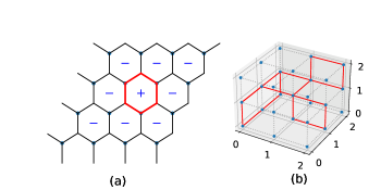
Figure 1: (Color online) (a) On a honeycomb lattice, a loop denoted by red bonds forms with the number of clusters $n_{c}=2$ and and the number of loops $l=1$ (b) For the cubic lattices, the graph may not satisfy the the planarity, required by the relationship $n_{c}=l+1$.

Starting at the partition function of the loop model,

$$Z_{\text{loop}}=\sum_{G}x^{b}n^{l},$$ (1)

where $l$ is the number of loops. The loop configuration on the honeycomb lattice can be represented by the Ising configuration on the triangular lattice (dual lattice of the honeycomb lattice), and the loops are just the domain walls [24, 25] of the Ising clusters. The number of the Ising clusters $n_{c}$ is just the number of loops $l$ plus 1, namely $n_{c}=l+1$.

For the honeycomb lattices, intersecting loops does not emerge as shown in Fig. 1 (a). The reason is that each configuration consists Eulerian-bond graph, “Eulerian“ means each site (vertex) is connected to even number of bonds.

However, for the square lattice, similar to the cubic lattice show in Fig. 1 (b), loop intersecting will occur. This will cause difficulties in counting the number of loop during simulations. Not only square lattice, any lattices with degree more than 3 will cause such confusion. Namely, each site connects more than 3 sites.

One way to solve such a question is not using the term “number of loops” in Eq (1) because such a quantity is not well defined on graphs with degree above 3. The correct term is “cyclomatic number”, defined to be the minimum number of edges required to be deleted from a graph in order to obtain a forest [28]. The value of “cyclomatic number” is $l=e-n+1$, where $e$ and $n$ are the numbers of bonds and the sites in the lattices, respectively. On graphs of maximum degree 3, the cyclomatic number does indeed count the number of loops $l$.

On the other hand, even using the definition of “cyclomatic number” $l$, the relation $n_{c}=l+1$ still holds for the square and honeycomb lattices, but this is only true for planar graphs. The requirement of planarity is very crucial. For the cubic lattices, the graph may not satisfy the requirement.

Here, we propose to performing direct research in the language of Ising clusters in the dual lattices rather than loop language. The partition function of the CWI model proposed reads,

$$Z_{\text{CWI}}=\sum_{\{S_{i}\}}\exp(-H)n^{n_{c}},$$ (2)

with the reduced Hamiltonian of the well known Ising model,

$$H=-K\sum\limits_{<i,j>}S_{i}S_{j},$$ (3)

where $K=J/k_{B}T$. The term $n^{n_{c}}$ is factor of cluster weight, and $n_{c}$ is the number of Ising clusters in the configurations and $n$ is a real number. The clusters are formulated by the connected spins with same directions.

The exploration of the CWI model will help to understand the loop model. By doing similar work like the low temperature expansion [29], the above model can be transformed into the loop model with the relation $x=\exp(-2K)$ between the parameters $x$ and $K$. The study of the CWI model will helps to understand $n$-component face cubic model [10, 9, 11], whose partition is which can transformed into a loop model.

III Algorithm and observables

The algorithm to simulate this model is as follows:

1. Initialize randomly assigned configuration.

2. Construct the Ising clusters: for a pair neighborhood sites $i$ and $j$ , if $S_{i}=S_{j}$, then absorb site $j$ into to the cluster.

3. Assign each Ising cluster with a green color(active) with a probability of $1/n$, but for a cluster with a red color(inactive) with a probability of $1-1/n$.

4. Construct the Swendsen-Wang clusters: for the site $i$, add its neighborhood site $j$ into the cluster according the rules as follows:

   1. No matter what the statuses of the spins on the sites $i$ and $j$ are, the only consideration is the color assigned on the sites. If one site in the site $i$ and $j$ is in red, then absorb the site $j$ into the cluster absolutely.

   2. If both sites $i$ and $j$ are in green, then absorb site $j$ into to the cluster with a probability of $p=1-e^{-2K}$ if $S_{i}=S_{j}$.

5. Flip the clusters with a probability $1/2$.

This algorithm is precisely introduced in Ref [23]. In this paper, we only apply it to non-planar graphs. Meanwhile, it would be worth mentioning that there is no particular reason to use Swendsen-Wang algorithm for the Ising updates on the active subgraph in step 4. Actually, “any” valid Ising Monte Carlo method would suffice, such as worm algorithm  [30], or Sweeny algorithm [31], or dynamic connectivity checking algorithm  [32].

Considered that we assign the clusters by red color (inactive) with a probability of $1-1/n$, and hence the algorithm we used only works for $n\geq 1$ even though the CWI model is well defined for any $n>0$.

With the help of Monte Carlo algorithm introduced before, the sampled observables include the magnetization $m$, the magnetic susceptibility $\chi$, the specific heat $C_{V}$ and the Binder ratio $Q$, which are defined as follows

$$m = \mathcal{\langle|M|\rangle},$$ (4)

$$Q = {\langle\mathcal{M}^{2}\rangle}^{2}/{\langle\mathcal{M}^{4}\rangle},$$ (5)

$$\chi = \frac{L^{3}}{k_{B}T}[{\langle\mathcal{M}^{2}\rangle}-{\langle\mathcal{M}\rangle}^{2}],$$ (6)

$$C_{V} = \frac{1}{{k_{B}}T^{2}}[{\langle E^{2}\rangle}-{\langle E\rangle}^{2}],$$ (7)

with ${M}$ defined as

$$\mathcal{M}={\sum_{i}S_{i}}/{L^{3}}.$$ (8)

The previous physical quantities have their scaling behavior as a function of the system size $L$ and the thermodynamic temperature $T$:

$$m= L^{y_{m}-d}[m_{0}+a_{1}(T-T_{c})L^{y_{t}}+a_{2}(T-T_{c})^{2}L^{2{y_{t}}}$$ (9)

$$+\cdots+b_{1}L^{y_{1}}+b_{2}L^{y_{2}}+\cdots],$$

$$Q= Q_{0}+e_{1}(T-T_{c})L^{y_{t}}+e_{2}(T-T_{c})^{2}L^{2{y_{t}}}$$ (10)

$$+\cdots+f_{1}L^{y_{1}}+f_{2}L^{y_{2}}+\cdots,$$

where ${T_{c}}$ is the critical temperature, ${y_{t}}$ is the thermal exponent, ${y_{m}}$ is the magnetic exponent, $d$ is the space dimension and ${y_{1}}$, ${y_{2}}$,$\cdots$, are negative correction-to-scaling exponents. The expansion coefficients $a_{i}$, $b_{i}$, $e_{i}$, $f_{i}$, ($i$ = 1, 2,$\cdots$) emerging in the two scaling functions, in general, are different.

The fitting function in Eq. (9) describes how $m$ depends on the expansion coefficients, and at the critical points, the function is reduced to

$$m=L^{y_{m}-d}(m_{0}+b_{1}L^{y_{1}}+b_{2}L^{y_{2}}+\cdots),$$ (11)

which will be used to determine the exponent ${y_{m}}$.

IV Results

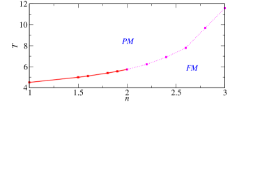
Figure 2: (Color online) The global phase diagram in the plane $T_{c}$ .vs. $n$, containing FM and PM phase. The dashed (solid) lines denote first (second order) transition.

Firstly, by the algorithm describing in Sec. III, we perform a Monte Carlo simulation of the CWI model on the 3D lattice. The first $10^{5}-10^{6}$ MC steps of simulation is performed in order to let the system reaches equilibrium states. Then ${10}^{5}$ samples in each thread (totally 100 threads) are taken to calculate each quantity for the system size $16{\leq}L{\leq}144$. The estimated auto correlation time $\tau_{int}$ is about $L^{0.45(3)}$ explained in Sec. IV.4. Therefore there are enough independent samples in the total $10^{7}$ samples. To obtain ${T_{c}}$ and ${y_{t}}$, we perform a finite-size scaling analysis of $Q$ for various system sizes near ${T_{c}}$. At $T_{c}$, $y_{m}$ is calculated.

IV.1 Global phase diagram and exponents

To verify our method and results, we first simulate the model with $n=1$ on the 3D lattice equivalent to the 3D Ising model, whose critical point is known at $T_{c}=4.5110(3)$ [33]. Our result $T_{c}$=4.5115(1) from the Binder ratio $Q$ according to Eq. (10) is consistent with results in Ref. [33]. Apart from the critical points, $y_{t}$ and $y_{m}$ are also very consistent with the results in Ref. [20]. We obtain $y_{t}=1.584(4)$ while $y_{t}$ takes value of $1.588(2)$ in Ref. [20].

The numerical exponents ${y_{t}}$ and ${y_{m}}$ at the critical points are listed in Table 1 for different values of $n$. The numerical estimation of $y_{t}$ and $y_{m}$ are different from with values in Ref [20] for $n$ = 1.5.

Table 1: Comparison of the numerical exponents with those in Ref [20]. The critical temperature ${T_{c}}$, the thermal exponent ${y_{t}}$ and the magnetic exponent ${y_{m}}$ for different values of $n$. The estimated errors in the last decimal place are shown between parentheses.

$n$	$T_{c}$	$y_{t}$	$y_{t}$$\rightarrow$Ref [20]	$y_{m}$	$y_{m}$$\rightarrow$Ref [20]
1.0	4.5115(1)	1.584(4)	1.588(2)	2.487(1)	2.483(3)
1.5	4.99912(5)	1.639(6)	1.538(4)	2.400(5)	2.482(3)
1.6	5.12147(5)	1.71(5)	-	2.34(2)	-
2.0	5.7514(2)	2.95(5)	1.488(3)	-	-

Fig. 2 shows the global phase diagram containing paramagnetic (PM) phase and ferromagnetic (FM) phase, where the dashed line denotes the first order transition in the range $n_{c}\leq n<3$ and the solid line represents the second order transition in the range $1<n<n_{c}$, where $n_{c}\approx 2$.

To summary, for $n>1$ on the 3D lattice, the universalities of the CWI model and the O($n$) loop model are different.

IV.2 $n=1,1.5$, detailed analysis

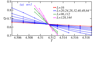
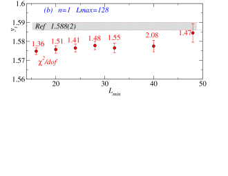
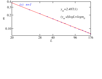
Figure 3: (Color online) (a) Binder ratio $Q$ .vs. $T$ at $n=1$ with different sizes. The critical point is ${T_{c}}=4.5115(1)$, and $Q_{0}=0.62(4)$. (b) $y_{t}$ .vs. $L_{min}$. The values of $\chi^{2}/dof$ are labeled. (c)The log-log plot of the magnetization $m$ .vs. $L$.

For $n=1$, the CWI model is reduced to the pure Ising model, which has been simulated in a higher precision by Ref [34]. It provides a good reference to check our result. To perform Levenberg-Marquardt(LM) least-squares fit [35], the weighted distance between data points and fitting function is defined as $\Delta_{i}=Q(T_{i};\{a_{n}\})-Q_{i}$, where ${a_{n}}$ is the parameter to be fitted including the exponents $y_{t}$, $y_{1}$, $y_{2}$, the coefficients $e_{1}$, $e_{2}$, $f_{1}$, $f_{2}$ and other quantities $Q_{0}$ and $T_{c}$. In practical, the error, i.e., standard deviation $\sigma_{i}$ of the data points $Q_{i}$ is divided aiming to minimise the quadratic distance,

$$\chi^{2}=\sum_{i=1}^{N}\frac{\Delta_{i}^{2}}{\sigma_{i}^{2}}=\sum_{i=1}^{N}\frac{[Q(T_{i};\{a_{n}\})-Q_{i}]^{2}}{\sigma_{i}^{2}}.$$ (12)

Figure 3(a) show the lines $Q$ .vs. $T$ in the regimes of $T_{c}$ in the range $4.506<T<4.518$ with various system sizes from $L=16-144$. Using the data $Q$ .vs. $T$ beginning with different values of $L_{min}=16,\cdots,48$ and the fixed maximum size $L_{max}=144$, the critical temperature is obtained as $T_{c}=4.5115(1)$, which is consistent with a more precise value $1/T_{c}=0.221654626(5)$ [34].

In Fig. 3 (b), the red symbols $y_{t}$ is obtained by fitting the terms including one corrected term $f_{1}L^{y_{1}}$. Increasing $L_{min}$, $y_{t}$ gradually converges to a value $y_{t}=1.584(4)$ consistent to the known result $y_{t}=1.588(2)$  [20] within the error bars when $L_{min}=48$. The goodness of fit $\chi^{2}$ per degree is distributed in an acceptable range between 1.36 and 2.08. In Fig. 3 (c), the magnetic exponent $y_{m}=2.487(1)$ is consistent with the results $y_{m}=2.483(3)$ in Ref [20] according to Eq. (9).

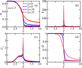
Figure 4: (Color online) (a) $m$ (b) ${\chi}$ (c) ${C_{V}}$ (d) $Q$ .vs. $T$ at $n=1.5$ in the range $0<T<10$, with different sizes $L=4,8,16$ and $32$, respectively.

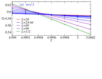
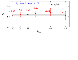
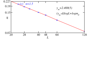
Figure 5: (Color online) (a)The Binder ratio $Q$ versus $T$ at $n=1.5$ with different sizes. (b) $y_{t}$ versus $L_{min}$. (c) The log-log plot of $m$ versus $L$.

For $n=1.5$, to get the the regime of the critical point, Figure 4 shows the magnetization $m$, the magnetic susceptibility ${\chi}$, the specific heat ${C_{V}}$ and the Binder ratio $Q$ as a function of $T$ with different system sizes $L=4,8,16$ and $32$. From the position of peaks and jumps, $T_{c}$ is around 5.

Precise $T_{c}$ is obtained by fitting Eq. (10). In Fig. 5(a), $Q~{}.vs.~{}T$ is calculated in a very narrow region ${4.9990<T<5.0002}$ with many different sizes $L=4-144$ and the the precise critical point is obtained at ${T_{c}}$=4.99912(5) by the LM algorithm. Correspondingly, the thermal exponent is ${y_{t}}$=1.639(6). This value is obtain by calcuate the average of $y_{t}$ through different $L_{min}$, the $\chi^{2}/dof$ is also shown in Fig. 5(b). The obtained $y_{t}$ is different from ${y_{t}}$=1.538(4) in Ref. [20]. This means that CWI model is not in the same universality as the pure loop model  [20].

Figure 5(c) shows the log-log plot $m$ versus system size $L$, i.e., $\log(m)=(y_{m}-d)\log(L)+\log(m_{0})$ for $n=1.5$ of the CWI model. The fitted result $y_{m}=2.400(5)$ is different from 2.482(3) in the last two significant digits.

IV.3 $n=2,3$, a first-order phase transition

We gradually increase $n$ in the range $2\leq n<3$. Since first-order transitions are difficult to study, we first consider simulating significantly larger $n$ values, which should be safely in the strongly first-order regime. The methods used are ploting the hysteresis and histogram of $m$ and $E$ [44, 45, 46], and check whether or not the exponent of $y_{t}$ equals to $d$. For $n=2$, histogram and fitting of Eq. (10) are used. The results by different methods check for each other.

IV.3.1 $n=3$

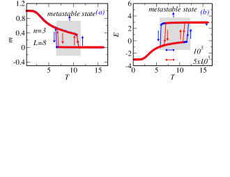
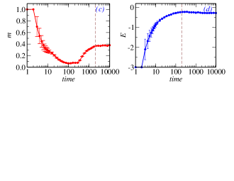
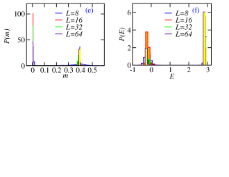
Figure 6: (Color online) (a) Hysteresis loop of the quantity $E$ .vs. $T$ (b) the quantity $Q$ .vs. $T$ (c) $m$ (d) $E$ vs. MC time at $T=10$. (e) Double-peak distributions of $m$ at $n=3$, with different sizes $L$ =8, 16, 32 and 64. (f) Double-peak distributions of $E$ at $n=3$, with different sizes $L$ =8, 16, 32 and 64 for $T=$11.8, 11.7, 11.6 and $11.3$.

To show the signature of a first-order transition for sufficiently large $n=3$, we draw the hysteresis loops of the energy and magnetization in Fig. 6(a) in the range $0<T<15$. The expression for the energy $E$ is

$$E=\frac{[-J\sum_{\langle i,j\rangle}S_{i}S_{j}-{n_{c}}\log(n)]}{L^{3}},$$ (13)

where $n_{c}$ is the number of Ising clusters in a spin configuration. The hysteresis loops have been observed both in classical Baxter-Wu model [36] and the site random cluster model [40], as well as quantum systems [37, 38, 39], which means that there is an obvious first-order phase transition [41, 42].

Although SW algorithm has a global update advantage, but it still has slow mixing for a first-order transition regime proved by Ref. [43], which can be used to form a closed hysteresis loop. Initializing with the temperature $T=0$, we increase $T$ as well as sample the energy per site $E$. In the simulation of a given value of “$T$”, we treat the spin configuration of the completed simulation, as the (new) initial configuration of the simulation of next value of “$T$”. After $T$ exceeds $T_{c}$ by a small value, the energy per site $E$ jumps to a higher value. We decrease $T$ in the same way with regards to the initialization of configurations. A closed hysteresis loop shapes when $T$ becomes smaller than $T_{c}$. We repeat these steps in a similar fashion for $m$, and the loop is shown in Fig. 6(b).

The hysteresis loops are caused by the fact that the lifetimes of the meta-stable states are much longer than the time intervals between temperature variations [36], and simulation and the measurements are taken from meta-stable states, marked by the gray area.

To confirm above statement, the quantity $\textless m(t)\textgreater=\frac{1}{t}\sum_{l=1}^{t}m(l)$ is also measured, where $m(l)$ is the observable $m$ observed at time $l$ in the Monte Carlo simulations. $E(t)$ is defined in the same way. As shown in Fig. 6 (c) and (d), $m(t)$ and $E(t)$ converge to 0.38013(1) and -0.27634(2) respectively, which are belong to the values of one metastable state.

For an infinite system with size $L\rightarrow\infty$, there will be a discontinuity at $T_{c}$ of order parameter $m$  [41]. For a finite system, the probability $p(m)$ is approximated by two Gaussian curves [42]. As shown in Figs. 7 (e) and (f), there are clearly double-peak structures at sizes $L=$ 32 and 64 for the histogram of $m$ and $E$. The sharp double-peak at $n=3$ is indicative of sufficiently strong first-order transition.

IV.3.2 $n=2$

Theoretically, for a first order transition, the fitting of Eq. (10) can not help determine $T_{c}$[41]. However, when finite system sizes are small and the temperatures become very close to $T_{c}$, Eq. (10) is used here to determine $y_{t}$. Figure 7(a) show the lines $Q$ .vs. $T$ in the regimes of $T_{c}$ in the range $5.7502<T<5.7532$ with various system sizes from $L=16-48$. By performing the LM algorithm, the values of goodness of fit $\chi^{2}/dof$ are acceptable and the values are shown in Figs 7(b). By sum over $y_{t}$ with different values of $L_{m}in$, the average $y_{t}$ is obtained as 2.95(5) indicating the scaling dimension $y_{t}$ equals to the space dimension $d$, i.e., $y_{t}=d$. This result is consistent with the conclusions in Refs [44, 45, 46].

In Figs 7 (c) and (d), the double-peak distributions of $m$ and $E$ at $n=2$ are shown, with different sizes $L$=32, 64, 96 for $T=$5.755, 5.7518 and 5.7516. Increasing the system sizes, the peaks become sharper representing that a first-order transition occurs.

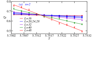
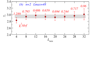
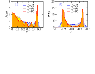
Figure 7: (Color online) (a)The Binder ratio $Q$ versus $T$ at $n=2$ with different sizes. (b) $y_{t}$ versus $L_{min}$. (c) Double-peak distributions of $m$ at $n=2$, with different sizes $L$=32, 64, 96. (d) Double-peak distributions of $E$ at $n=2$, with different sizes $L$=32, 64, 96 for $T=$5.755, 5.7518 and 5.7516.

IV.4 Autocorrelation function

The algorithm has a little critical slowing down phenomenon. This phenomena can be judged by autocorrelation time $\tau_{int}$, which can identify the number of MC steps required between two configurations before they can be considered statistically independent [47].

For the quantity absolute magnetism $M=|\mathcal{M}|$, the integrated autocorrelation function $A_{M}(t)$ is defined as:

$$A_{M}(t)=\frac{\langle M_{k}M_{k+t}\rangle-\langle M_{k}\rangle^{2}}{\langle M_{k}^{2}\rangle-\langle M_{k}\rangle^{2}}$$ (14)

and the integrated accucorrelation time $\tau_{int}$ is defined as

$$\tau_{int}=\frac{1}{2}+\sum_{t=0}^{\infty}A_{M}(t)$$ (15)

In Figs. 8(a) and (b), the autocorrelation function $A_{m}(t)$ for the $M$ decays almost purely exponentially on MC time (a linear decay on the linear-log scale). Close to $T_{c}=0.499912$, $A_{M}(t)$ grows with $L$ while it decreases with $L$ when the temperature deviates away from $T_{c}$.

As shown in Fig. 8(c), the integrated autocorrelation time $\tau_{int}$ behaviors in the way like $L^{z}$ at $T=T_{c}$ where the dynamical exponent $z=0.45(3)$ and the error bar in the parentheses is the systematic error due to corrections to scaling [48]. This value of $z$ is consistent (within error bar) with the result 0.443±0.005±0.030 of a “susceptibility-like” observable, or 0.459±0.005±0.025 of a “energy like” observable from Ref. [48] studying the three dimensional Ising model by the SW algorithm [22]. The algorithm we used for $n=1.5$ is as efficient as the SW algorithm.

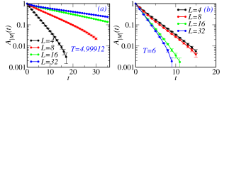
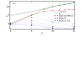
Figure 8: (Color online) $A_{M}(t)$ versus $t$ for $n=1.5$ CWI model with different sizes at (a) $T=T_{c}$ (b) $T=6>T_{c}$. (c) $\tau_{int}$ versus $L$ at different temperatures. The exponent $z$ is fitted to be $z=0.45(3)$.

IV.5 Error bar analysis

The programs are run in 100 threads (bins), and in each thread (bin) different seed of random number generator is used. The first $10^{5}-10^{6}$ MC steps of simulations are run without measuring any quantities allowing the systems to reach the stage of equilibrium. $10^{7}$ times of sampling are performed in the equilibrium states and the mean values of the quantities are collected from each bin.

For example, the quantity $m$ is average from many bins according to $m=\frac{1}{nbin}\sum_{b=1}^{nbin}\overline{m}_{b}$, where $\overline{m}_{b}$, $b=1,\cdots,nbin$ are computed over each bin. The error bar $\sigma$ is calculated according to

$$\sigma=\sqrt{\frac{1}{nbin(nbin-1)}\sum_{b=1}^{nbin}(\overline{m}_{b}-m)^{2}}$$ (16)

The quoted error bar corresponds to one standard deviation (i.e., confidence level $\approx 68\%$).

The error bars of the fitted exponents are estimated by the diagonal elements of the covariance matrix $[C]=[\alpha]^{-1}$, where $\alpha$ is defined by [35]

$$\alpha_{kl}=\sum_{i=1}^{N}\frac{1}{\sigma_{i}^{2}}\left[\frac{\partial Q(T_{i};\{a_{n}\})}{\partial a_{k}}\frac{\partial Q(T_{i};\{a_{n}\})}{\partial a_{l}}\right]$$ (17)

V Discussion and conclusion

It should be noted that, loop model can be obtained as a high-temperature expansion of various cubic models, such as both face and corner cubic model  [4], in which the spins point to the corners of an $n$-dimensional hypercube, but it also arises as a high temperature expansion of the O($n$) vector spin model in certain settings. The descriptor cubic or O($n$) refers to a symmetry of the spin Hamiltonian, and has no immediate interpretation in the loop language. Furthermore, the face cubic and corner cubic models can both be related to this same loop model but can have entirely different phase transitions [4].

In conclusion, we have proposed a cluster weight Ising (CWI) model, composed of an Ising model with an additional cluster weight in the partition function with respect to the traditional Ising model. In order to simulate the CWI model, we apply an efficient cluster algorithm by combining the color-assignation and the Swendsen-Wang method. The algorithm has almost the same efficiency as the Swendsen-Wang method, i.e., the dynamical exponent for the absolute magnetization $z=0.45(3)$ at $n=1.5$ is consistent with that of the traditional Swendsen-Wang method.

Second order transitions emerges with $1\leq n<n_{c}$ and first order transitions occur when $n\geq n_{c}$ ($n_{c}\approx 2$) of the CWI model on the 3D lattices, and the universalities of our CWI model and the loop model [20] are completely different. The first-order transition is verified by the signatures of hysteresis, double-peak structure of histograms for the order parameters, and the value of the critical exponent $y_{t}=d$. Our results can be helpful in the understanding of traditional statistical models.

References

- [1] E. Ising, Beitrag zur theorie des ferromagnetismus, Z. Phys. 31, 253 (1925).
- [2] H. E. Stanley, Dependence of Critical Properties on Dimensionality of Spins , Phys. Rev. Lett. 20, 589 (1968).
- [3] D. Kim and P. M. Levy, Critical behavior of thr cubic model, Phys. Revs. B. 12, 5105(1975).
- [4] B. Nienhuis, E. K. Riedel and M. Schick, Critical behavior of the n-component cubic model and the Ashkin-Teller fixed line, Phys. Rev. B. 27, 5625(1983).
- [5] K. Nagai, Phase diagrams of the corner cubic Heisenberg model and its site-diluted version on a triangular lattice: Renormalization-group treatment, Phys. Rev. B. 31, 1570 (1984).
- [6] A. M. P. Silva, A. M. J. Schakel, and G. L. Vasconcelos, Critical line of the O() loop model on the square lattice, Phys. Rev. E 88, 021301 (2013).
- [7] W. A. Guo, H. W. J. Blöte, and B. Nienhuis, Phase diagram of a loop on the square lattice, Int. J. Mod. Phys. C 10, 301 (1999).
- [8] Z. Fu, W. A. Guo, and H. W. J. Blöte, Ising-like transitions in the O() loop model on the square lattice, Phys. Rev. E 87, 052118 (2013).
- [9] W. A. Guo, X. F. Qian, H. W. J. Blöte, and F. Y. Wu, Critical line of an n-component cubic model, Phys. Rev. E 73, 026104 (2006).
- [10] C. X. Ding, G. Y. Yao, S. Li, Y. J. Deng, and W. A. Guo, Universal critical properties of the Eulerian bond-cubic model, Chin. Phys. B 20, 070504 (2011).
- [11] C. X. Ding, W. A. Guo, and Y. J. Deng, Ising-like phase transition of an n-component Eulerian face-cubic model, Phys. Rev. E 88, 052125 (2013).
- [12] B. Nienhuis, Exact critical point and critical exponents of O() models in two dimensions, Phys. Rev. Lett. 49, 1062 (1982).
- [13] V. L. Berezinskii, Destruction of long-range order in one-dimensional and two-dimensional systems having a continuous symmetry group . classical systems, Sov. Phys. JETP 32(3), 493 (1971).
- [14] J. M. Kosterlitz and D. J. Thouless, Ordering, metastability and phase transitions in two-dimensional systems, J. Phys. C 5, L124 (1972).
- [15] J. M. Kosterlitz, The critical properties of the two-dimensional xy model, J. Phys. C 7, 1046 (1974).
- [16] C. X. Ding, X. F. Qian, Y. J. Deng and H. W. J. Blöte, Geometric properties of two-dimensional O() loop configurations, J. Phys. A: Math. Theor. 40, 3305(2007).
- [17] W. A. Guo, H. W. J. Blöte, and F. Y. Wu, Phase transition in the Honeycomb O() model, Phys. Rev. Lett. 85, 3874 (2000).
- [18] H. W. J. Blöte and M. P. Nightingale, The temperature exponent of the -component cubic model, Physica A 129 , 1 (1984).
- [19] C. X. Ding, H. W. J. Blöte, and Y. J. Deng, Emergent O() symmetry in a series of 3D Potts models, Phys. Rev. B. 94, 104402 (2016).
- [20] Q. Q. Liu, Y. J. Deng, T. M. Garoni, and H. W. J. Blöte, The O() loop model on a three-dimensional lattice, Nucl. Phys. B 859, 107 (2012).
- [21] J. M. Carmona, A. Pelissetto, and E. Vicari, N-component Ginzburg-Landau Hamiltonian with cubic anisotropy: A six-loop study, Phys. Rev. B 61, 15136 (2000).
- [22] R. H. Swendsen, J. S. Wang, Nonuniversal critical dynamics in Monte Carlo simulations, Phys. Rev. Lett. 58 86 (1987).
- [23] Y. J. Deng, T. M. Garoni, W. A. Guo, H. W. J. Blöte, and A. D. Sokal, Cluster simulations of loop models on two-dimensional lattices, Phys. Rev. Lett. 98, 120601 (2007).
- [24] J. Dubail, J. L. Jacobsen, and H. Saleur, Critical exponents of domain walls in the two-dimensional Potts model, J. Phys. A: Math. Theor. 43, 482002 (2010).
- [25] C. X. Ding, X. F. Qian, Y. J. Deng, W. A. Guo, and H. W. J. Blöte, Geometric properties of two-dimensional O() loop configurations, J. Phys. A: Math. Theor. 40, 3305 (2007).
- [26] Q. Q. Liu, Y. J. Deng, and T. M. Garoni, Worm Monte Carlo study of the honeycomb-lattice loop model, Nucl. Phys. B 846, 283 (2011).
- [27] Y. D. Xu, Q. Q. Liu, and Y. J. Deng, Monte Carlo study of the universal area distribution of clusters in the honeycomb O() loop model, Chin. Phys. B 21, 070211 (2012).
- [28] K. J. Cohn, Cyclomatic numbers of planar graphs, Discrete. Math. 178, 245 (1998).
- [29] G. Bhanot, M. Creutz, and J. Lacki, Low-temperature expasion for the Ising model, Phys. Rev. Lett. 69, 1841 (1992).
- [30] N. Prokofiev’ev, B. Svistunov, Worm Algorithms for Classical Models, Phys. Rev. Lett. 87,160601 (2001).
- [31] M. Sweeny, Monte Carlo study of weighted percolation clusters relevant to the Potts models, Phys. Rev. B. 27, 4445(1983). M. Sweeny, Monte Carlo study of weighted percolation clusters relevant to the Potts models, Phys. Rev. B. 27, 4445(1983).
- [32] E. M. Elçi and M. Weigel, Dynamic connectivity algorithms for Monte Carlo simulations of the random-cluster model, J Phys Conf Ser, 510 012013 (2014).
- [33] K. Binder and E. Luijten, Monte carlo tests of renormalization-group predictions for critical phenomena in Ising models, Phys. Rep. 344, 179 (2001).
- [34] A. M. Ferrenberg, J. H. Xu, D. P. Landau, Pushing the limits of Monte Carlo simulations for the three-dimensional Ising model, Phys. Rev. E. 97,043301 (2018).
- [35] D. W. Marquardt, An algorithm for least-squares estimation of nonlinear parameters, J. Soc. Indust. Appl. Math. 11(2), 431 (1963).
- [36] Y. J. Deng, W. A. Guo, J. R. Heringa, H. W. J. Blöte, and B. Nienhuis, Phase transitions in self-dual generalizations of the Baxter-Wu model, Nucl. Phys. B 827, 406 (2010).
- [37] W. Z. Zhang, R. X. Yin, and Y. C. Wang, Pair supersolid with atom-pair hopping on the state-dependent triangular lattice, Phys. Rev. B 88, 174515 (2013).
- [38] W. Z. Zhang, R. Li, W. X. Zhang, C. B. Duan, and T. C. Scott, Trimer superfluid induced by photoassociation on the state-dependent optical lattice, Phys. Rev. A 90, 033622 (2014).
- [39] W. Z. Zhang, Y. Yang, L. J. Guo, C. X. Ding, and T. C. Scott, Trimer superfluid and supersolid on two-dimensional optical lattices, Phys. Rev. A 91, 033613 (2015).
- [40] S. S. Wang, W. Z. Zhang, and C. X. Ding, Percolation of the site Random-Cluster model by Monte Carlo method, Phys. Rev. E 92, 022127 (2015).
- [41] D. P. Landau and K. Binder, A Guide to Monte Carlo Simulations in Statistical Physics (Cambridge University Press, 2006).
- [42] K. Binder and D. P. Landau, Finite-size scaling at first-order phase transitions, Phys. Rev. B 30, 1477 (1984).
- [43] V. K. Gore and M. R. Jerrum, The Swendsen-Wang process does not always mix rapidly, J. Stat. Phys. 97, 67(1999).
- [44] M. E. Fisher and A. N. Berker, Scaling for first-order phase transitions in thermodynamic and finite systems, Phys. Rev. B 26, 2507 (1982).
- [45] K. Vollmayr, J. D. Reger, M. Scheucher, and K. Binder, Finite size effects at thermally-driven first order phase transitions: A phenomenological theory of the order parameter distribution, Z. Phys. B 91, 113 (1991).
- [46] J. Lee and J. M. Kosterlitz, Finite-size scaling and Monte Carlo simulations of first-order phase transitions, Phys. Rev. B 43, 3265 (1991).
- [47] A. W. Sandvik, Computational Studies of Quantum Spin Systems, AIP. Conf. Proc. 1297, 135(2010).
- [48] G. Ossola and A. D. Sokal, Dynamic critical behavior of the Swendsen-Wang algorithm for the three - dimensional Ising model, Nucl. Phys. B. 99, 110601 (2007).