Scalable Molecular GW Calculations: Valence and Core Spectra

Abstract

We present a scalable implementation of the $GW$ approximation using Gaussian atomic orbitals to study the valence and core ionization spectroscopies of molecules. The implementation of the standard spectral decomposition approach to the screened Coulomb interaction, as well as a contour deformation method are described. We have implemented both of these approaches using the robust variational fitting approximation to the four-center electron repulsion integrals. We have utilized the MINRES solver with the contour deformation approach to reduce the computational scaling by one order of magnitude. A complex heuristic in the quasiparticle equation solver further allows a speed-up of the computation of core and semi-core ionization energies. Benchmark tests using the GW100 and CORE65 datasets and the carbon 1s binding energy of the well-studied ethyl trifluoroacetate, or ESCA molecule, were performed to validate the accuracy of our implementation. We also demonstrate and discuss the parallel performance and computational scaling of our implementation using a range of water clusters of increasing size.

1 Introduction

Many-body perturbation theory (MBPT) has been extensively demonstrated^{1, 2, 3} over the years as a worthy alternative to density functional theory (DFT). This has resulted in a number of useful approximations that are widely used in solid-state physics and quantum chemistry. Specifically, within the framework of MBPT, the $GW$ approximation to the self-energy $\Sigma$⁴, has been used with considerable success over the last three decades and has widespread reputation as an accurate and efficient method for the prediction of band-structures in solids. In recent years there has been growing interest in the $GW$ method applied to molecular and finite systems (see reviews 5, 6, 7, 8, 9, 10 and references therein).

The $GW$ quasi-particle energies, unlike the Kohn-Sham (KS) single-particle energies, can be used to calculate properties associated with charged excitations (i.e. electron addition and removal) that can be compared to photoemission and inverse-photoemission spectroscopy. Other key features include the absence of empirical parameters, ab initio inclusion of dynamical electron correlation, appropriate long range behavior of the electron-hole interaction and a well-defined physical meaning of the quasi-particle energies. In addition, the moderate computational cost of the $GW$ approach, between DFT and traditional quantum chemistry correlated approaches, makes it an attractive first-principles theory for charged excitation energies. The $GW$ quasi-particle energies also serve as a starting point to describe neutral transitions (for example, optical and x-ray absorption spectroscopies) via the Bethe-Salpeter (BSE) formalism ¹¹, which introduces electron-hole interaction effects at the same level of theory.

The simplest and most popular form of the $GW$ approximation is the first-order $G_{0}W_{0}$ approach, which is performed as a post-processing or one-shot step to a KS (local, semilocal, hybrid or pure Hartree-Fock (HF)) reference calculation. Here, the non-interacting Green’s function $G$ is diagonal in the KS (or HF) eigenstate basis, and only the diagonal matrix elements of the self-energy are needed to evaluate the quasi-particle energy corrections to first order. Some of the issues (for example, the KS or HF reference dependence) of the one-shot approach can be improved with different levels of refinement, such as the eigenvalue (ev) self-consistent approaches where the quasi-particle eigenvalues are used to iteratively update the Green’s Function $G$ (ev$GW_{0}$) or both $G$ and $W$ (ev$GW$) or the more complex self-consistent (sc) approaches, where both the orbitals and quasi-particle eigenvalues are calculated and iterated to self-consistency in $G$ (sc$GW_{0}$) or both $G$ and $W$ (sc$GW$), respectively.^{12, 13, 14} Consequently, the $GW$ approximation is now an integral part of electronic structure theory and is available in many widely used electronic structure codes like Turbomole ^{15, 16, 17, 18}, FHI-Aims ¹⁹ , CP2K ^{20, 21}, ADF ²², molGW ²³, BerkeleyGW²⁴, Quantum ESPRESSO^{25, 26, 27, 28}, Abinit²⁹, VASP^{30, 31, 32, 33}, Yambo ^{34, 35}, WEST³⁶, Elk ³⁷, PySCF ^{38, 39}, GPAW^{40, 41, 42}, WIEN2k ^{43, 44, 45}, Questaal ⁴⁶, Spex ⁴⁷.

In this paper, we describe our implementation of the $GW$ approximation based on the software infrastructure of the open-source NWChem computational chemistry program ⁴⁸ within the Gaussian basis set framework for molecular and finite systems. Our implementation can use either the spectral decomposition (SD) or the contour-deformation (CD) methods. Both approaches are suitable to describe valence and core ionization spectra. The rest of the paper is organized as follows: For completeness, in Section 2, we describe the theoretical framework of the $GW$ approximation and the theoretical background of both of the approaches we have implemented to obtain the screened Coulomb interaction. Section 3 describes the details of the implementation, with special emphasis on the contour deformation approach. Section 4 shows benchmark results for both core and valence ionizations by comparing with the GW100 ⁴⁹ and CORE65⁵⁰ datasets as well as computations of the carbon 1s binding energies of the ESCA molecule. Parallel scalability is presented and discussed in Section 5. Finally, a brief summary and outlook is presented in Section 6.

2 Theory

2.1 Overview of the Hedin Equations and Derivation of the $GW$ Approximation

The central object of the $GW$ theory is the one-particle Green’s function $G$ describing particle and hole scattering in the interacting many-body system. Formally $G$ is defined in terms of time-ordered products of creation ($\hat{\psi}^{\dagger}$) and annihilation ($\hat{\psi}$) operators in the Heisenberg representation ²

$$iG(1,2) =\langle\Psi_{0}|T[\hat{\psi}_{H}(1)\hat{\psi}^{\dagger}_{H}(2)]|\Psi_{0}\rangle$$

$$=\theta(t_{1}-t_{2})\langle\Psi_{0}|\hat{\psi}_{H}(1)\hat{\psi}^{\dagger}_{H}(2)|\Psi_{0}\rangle-\theta(t_{2}-t_{1})\langle\Psi_{0}|\hat{\psi}^{\dagger}_{H}(2)\hat{\psi}_{H}(1)|\Psi_{0}\rangle$$

where $|\Psi_{0}\rangle$ is an exact ground state satisfying the time-independent Schrödinger equation $H|\Psi_{0}\rangle=E_{0}|\Psi_{0}\rangle$, $i=1,2,...$ refers to a combined space-time coordinate $(r_{i},t_{i})$ and $\theta$ is the Heaviside step function under the half maximum convention. For simplicity, spin variables have been omitted in the above definition. The $GW$ approximation can be derived from the Hedin’s equations⁴ by substituting the vertex function $\Gamma$ with the product of the two delta functions $\Gamma(1,2,3)=\delta(1-2)\delta(2-3)$ which amounts to the first order approximation to the self-energy $\Sigma$ in terms of the screened Coulomb potential $W$:

$$\Sigma(1,2) =iG(1,2)W(1,2^{+}),$$ (1)

where “+” indicates chronological ordering (e.g. $t_{1}^{+}=t_{1}+\eta$, $\eta\to 0$). From a physical standpoint $W$ describes the interaction between dynamically screened quasi-particles as reflected in its definition in terms of the inverse dielectric function $\epsilon^{-1}(1,2)$ and bare Coulomb potential $v(1,2)=\delta(t_{1}-t_{2})\frac{1}{|r_{1}-r_{2}|}$ (assuming instantaneous and spin-independent interaction in the non-relativistic case)

$$W(1,2)=\int d3\epsilon^{-1}(1,3)v(3,2).$$ (2)

It can be shown that $W$ satisfies a Dyson-like equation

$$W(1,2) =v(1,2)+\int d(34)v(1,3)P(3,4)W(4,2),$$ (3)

connecting it to the irreducible polarizability $P$ describing the density response with respect to the total potential (accounting for both induced and external contributions):

$$P(1,2) =-iG(1,2)G(2,1^{+})$$ (4)

Along with the Dyson equation for the interacting Green’s function (in terms of the Hartree Green’s function, $G_{H}$)

$$G(1,2) =G_{H}(1,2)+\int d(34)G_{H}(1,3)\Sigma(3,4)G(4,2)$$ (5)

equations 1, 4, and 3 form the basis of $GW$ approach. The crux of $GW$ is the evaluation of the screened Coulomb interaction $W(1,2)$ which can, in principle, be obtained by solving Eq. 3. In practical applications it is more efficient to express $W$ in terms of the reducible polarizability, or density response function, $\chi$ describing the perturbation of the electronic density by a time- dependent external potential:

$$\chi(1,2)=P(1,2)+\int d(34)P(1,3)v(3,4)\chi(4,2)$$ (6)

Combining the above equation with 3 one effectively obtains a closed form expression for $W$ in terms of $\chi$ the high quality approximations which are available in standard electronic structure packages:

$$W(1,2) =v(1,2)+\int d(34)v(1,3)\chi(3,4)v(4,2)$$ (7)

In the non-relativistic case Eq. 7 can be further simplified:

$$W(1,2) =v(r_{1},r_{2})\delta(t_{1}-t_{2})+\int d(r_{3}r_{4})v(r_{1},r_{3})\chi(r_{3},r_{4};t_{1}-t_{2})v(r_{4},r_{2})$$ (8)

In the frequency domain the equation for the self-energy is transformed as follows:

$$\Sigma(r_{1},r_{2},\omega)=\frac{i}{2\pi}\int_{-\infty}^{+\infty}e^{i\xi\eta}G(r_{1},r_{2},\omega+\xi)W(r_{1},r_{2},\xi)d\xi,$$ (9)

under the usual assumption of $\eta\to 0^{+}$. Combining the previous equation with the expression for screened Coulomb interaction one obtains:

$$\Sigma(r_{1},r_{2},\omega)=\frac{i}{2\pi}v(r_{1},r_{2})\int_{-\infty}^{+\infty}e^{i\xi\eta}G(r_{1},r_{2},\omega+\xi)d\xi\ +$$

$$\frac{i}{2\pi}\int_{-\infty}^{+\infty}d\xi\int d(r_{3}r_{4})e^{i\xi\eta}G(r_{1},r_{2},\omega+\xi)v(r_{1},r_{3})\chi(r_{3},r_{4};\xi)v(r_{4},r_{2})$$ (10)

where the first contribution can be readily recognized as an exchange part of the self-energy since $-\rho(r_{1},r_{2})=\frac{i}{2\pi}\int_{-\infty}^{+\infty}e^{i\xi\eta}G(r_{1},r_{2},\xi)d\xi$ is the one particle density matrix.

2.2 Spectral Decomposition

One way of obtaining $\Sigma(\omega)$ is via the spectral decomposition (SD) of the density response function $\chi$ in the random phase approximation (RPA):

$$\chi(r_{1},r_{2},\omega)=\sum\limits_{s}n_{s}(r_{1})n_{s}(r_{2})\left(\frac{1}{\omega-\Omega_{s}+i\eta}-\frac{1}{\omega+\Omega_{s}-i\eta}\right)$$ (11)

where $n_{s}$ are transition densities and $\Omega_{s}$ are the charge-neutral excitations. These can be obtained by solving the Casida equations:

$$\begin{bmatrix}A&B\\ -B&-A\end{bmatrix}\begin{bmatrix}X_{s}\\ Y_{s}\end{bmatrix}=\Omega_{s}\begin{bmatrix}X_{s}\\ Y_{s}\end{bmatrix},$$ (12)

where, for closed-shells, $A_{ia,jb}=\delta_{ij}\delta_{ab}(\epsilon_{a}-\epsilon_{i})+2(ia|jb)$, $B_{ia,jb}=2(ia|bj)$. The open-shell equations can be written by explicitly exposing the spin blocks as

$$\begin{bmatrix}A_{\uparrow\uparrow}&B_{\uparrow\uparrow}&B_{\uparrow\downarrow}&B_{\uparrow\downarrow}\\ -B_{\uparrow\uparrow}&-A_{\uparrow\uparrow}&-B_{\uparrow\downarrow}&-B_{\uparrow\downarrow}\\ B_{\downarrow\uparrow}&B_{\downarrow\uparrow}&A_{\downarrow\downarrow}&B_{\downarrow\downarrow}\\ -B_{\downarrow\uparrow}&-B_{\downarrow\uparrow}&-B_{\downarrow\downarrow}&-A_{\downarrow\downarrow}\end{bmatrix}\begin{bmatrix}X_{\uparrow}^{s}\\ Y_{\uparrow}^{s}\\ X_{\downarrow}^{s}\\ Y_{\downarrow}^{s}\end{bmatrix}=\Omega_{s}\begin{bmatrix}X_{\uparrow}^{s}\\ Y_{\uparrow}^{s}\\ X_{\downarrow}^{s}\\ Y_{\downarrow}^{s}\end{bmatrix},$$ (13)

and where $A_{ia\sigma,jb\sigma}=\delta_{ij}\delta_{ab}(\epsilon_{a\sigma}-\epsilon_{i\sigma})+\left(ia\sigma\big{|}jb\sigma\right)$ and $B_{ia\sigma_{1},jb\sigma_{2}}=\left(ia\sigma_{1}\big{|}jb\sigma_{2}\right)$.

The matrix elements of $W$ in the orbital product basis are then expressed in terms of the full set of eigenvectors $(X_{s},Y_{s})$ and corresponding neutral excitation energies $\Omega_{s}$:

$$W_{mn\sigma_{1},op\sigma_{2}}(\omega)=(mn\sigma_{1}|op\sigma_{2})+\sum_{s}\omega_{mn\sigma_{1}}^{s}\omega_{op\sigma_{2}}^{s}\times\big{(}\frac{1}{\omega-\Omega_{s}+i\eta}-\frac{1}{\omega+\Omega_{s}-i\eta}\big{)},$$ (14)

where $\omega_{mn\sigma}^{s}=\sum_{ia\sigma}(mn\sigma_{1}|ia\sigma)(X_{ia\sigma}^{s}+Y_{ia\sigma}^{s})$. Eq. 14 is a key component of the spectral decomposition approach and often serves as a starting point for deriving approximate $GW$ and BSE methods. In particular, the matrix elements of the self-energy can be directly obtained by contracting $W_{mn\sigma_{1},op\sigma_{2}}(\omega)$ with the KS Green’s function:

$$G_{\sigma\sigma\prime}^{KS}(r_{1},r_{2},\omega)=\delta_{\sigma\sigma\prime}\sum_{k}\frac{\phi_{k\sigma}(r_{1})\phi_{k\sigma}^{*}(r_{2})}{\omega-\epsilon_{k\sigma}+i\eta\times sign(\epsilon_{k\sigma}-\mu)}$$ (15)

with $\mu$ being the Fermi-level of the system.

Integration is performed by closing the contour in the upper half of the complex plane such that

$$\int_{-\infty}^{+\infty}\frac{d\xi e^{i\xi\eta}}{(\xi+\omega-\epsilon_{k\sigma}+i\eta\times sign(\epsilon_{k\sigma}-\mu))(\xi-\Omega_{s}+i\eta)}=\begin{cases}0&\mbox{if }\epsilon_{k\sigma}>\mu\\ -\frac{2\pi i}{\omega-\epsilon_{k\sigma}+\Omega_{s}-2i\eta}&\mbox{otherwise }\end{cases}$$

$$\int_{-\infty}^{+\infty}\frac{d\xi e^{i\xi\eta}}{(\xi+\omega-\epsilon_{k\sigma}+i\eta\times sign(\epsilon_{k\sigma}-\mu))(\xi+\Omega_{s}-i\eta)}=\begin{cases}\frac{2\pi i}{\omega-\epsilon_{k\sigma}-\Omega_{s}+2i\eta}&\mbox{if }\epsilon_{k\sigma}>\mu\\ 0&\mbox{otherwise }\end{cases}$$

The final expression for the self-energy in terms of tensor contractions is presented below:

$$\Sigma_{nn\sigma}(\omega)=\frac{i}{2\pi}\int_{-\infty}^{+\infty}d\xi e^{i\xi\eta}\sum\limits_{i}\frac{W_{ni\sigma,in\sigma}(\xi)}{\xi+\omega-\epsilon_{i\sigma}-i\eta}+\sum\limits_{a}\frac{W_{na\sigma,an\sigma}(\xi)}{\xi+\omega-\epsilon_{a\sigma}+i\eta}$$ (16)

$$=-\sum\limits_{i}(ni\sigma|in\sigma)+\sum\limits_{is}\frac{\omega_{ni\sigma}^{s}\omega_{in\sigma}^{s}}{\omega-\epsilon_{i\sigma}+\Omega_{s}-2i\eta}+\sum\limits_{as}\frac{\omega_{na\sigma}^{s}\omega_{an\sigma}^{s}}{\omega-\epsilon_{a\sigma}-\Omega_{s}+2i\eta}$$ (17)

The most expensive part of the spectral decomposition approach is the computation of the neutral excitations $\Omega_{s}$ and the associated eigenvectors $X_{s}$ and $Y_{s}$, which formally scales as $\mathcal{O}(N^{6})$. One way of avoiding this steep computational cost is by means of the contour-deformation technique described below.

2.3 Contour Deformation

Instead of using the density response function $\chi$ in order to obtain the screened Coulomb interaction, the contour deformation (CD) approach uses the independent-particle irreducible polarizability $\chi_{0}$, which has a simple sum-over-states representation ^{51, 52}. However, the integration in Eq. 10 can no longer be solved analytically. Following Ref. 53, the self-energy is decomposed as

$$\Sigma(r_{1},r_{2},\omega)=R(r_{1},r_{2},\omega)-I(r_{1},r_{2},\omega)$$ (18)

where the contour integral $R(r_{1},r_{2},\omega)$ and the integral over the imaginary axis $I(r_{1},r_{2},\omega)$ are defined as

$$R(r_{1},r_{2},\omega):=\frac{i}{2\pi}\oint d\xi\>G(r_{1},r_{2},\omega+\xi)W(r_{1},r_{2},\xi)$$ (19)

$$I(r_{1},r_{2},\omega):=\frac{1}{2\pi}\int\limits_{-\infty}^{\infty}d\xi\>G(r_{1},r_{2},\omega+i\xi)W(r_{1},r_{2},i\xi)$$ (20)

The contour integral is evaluated using the residue theorem by choosing the contours in such a way that only the poles of $G_{0}$ are enclosed, yielding

$$R(r_{1},r_{2},\omega)= - \sum\limits_{i}\phi_{i}(r_{1})\phi_{i}(r_{2})W(r_{1},r_{2},\epsilon_{i}-\omega+i\eta)\theta(\epsilon_{i}-\omega)$$ (21)

$$+ \sum\limits_{a}\phi_{a}(r_{1})\phi_{a}(r_{2})W(r_{1},r_{2},\epsilon_{a}-\omega-i\eta)\theta(\omega-\epsilon_{a})$$

The integral over the imaginary axis $I(r_{1},r_{2},\omega)$ is obtained by inserting Eq. 15 into Eq. 20,

$$I(r_{1},r_{2},\omega)=\frac{1}{2\pi}\sum\limits_{m}\int\limits_{-\infty}^{\infty}d\xi\frac{\phi_{m}(r_{1})\phi_{m}(r_{2})W(r_{1},r_{2},i\xi)}{\omega+i\xi-\epsilon_{m}+sign(\epsilon_{k}-\mu)}\;,$$ (22)

The diagonal matrix elements for the self-energy in the MO basis are then obtained as

$$\Sigma_{nn\sigma}(\omega) = -\sum\limits_{i}W_{ni\sigma,ni\sigma}(\epsilon_{i\sigma}-\omega+i\eta)\theta(\epsilon_{i\sigma}-\omega)$$ (23)

$$+\sum\limits_{a}W_{na\sigma,na\sigma}(\epsilon_{a\sigma}-\omega-i\eta)\theta(\omega-\epsilon_{a\sigma})$$

$$-\frac{1}{2\pi}\sum\limits_{m}\int\limits_{-\infty}^{\infty}d\xi\frac{W_{nm\sigma,nm\sigma}(i\xi)}{i\xi-\epsilon_{m\sigma}+sign(\epsilon_{k}-\mu)}$$

$$= R_{nn\sigma}(\omega)-I_{nn\sigma}(\omega)$$ (24)

3 Implementation

3.1 Variational Fitting Approximation

We have implemented the $GW$ and $evGW$ methods using the robust variational fitting (RVF) technique ^{54, 55, 56}. Within RVF, the two-particle four-center electron repulsion integral (ERI)

$$\left(ai\big{|}bj\right):=\iint d(r_{1}r_{2})\phi_{a}(r_{1})\phi_{i}(r_{1})v(r_{1},r_{2})\phi_{b}(r_{2})\phi_{j}(r_{2})$$ (25)

is approximated as

$$\left(ai\big{|}bj\right)\approx\left(\widetilde{ai}\big{|}bj\right)+\left(ai\big{|}\widetilde{bj}\right)-\left(\widetilde{ai}\big{|}\widetilde{bj}\right)$$ (26)

with

$$\widetilde{\phi_{i}(r)\phi_{a}(r)}:=\sum\limits_{P}C_{ia}^{P}f_{P}(r)$$ (27)

and $f_{P}(r)$ an atom-centered auxiliary function. The fitting coefficients $C_{ia}^{P}$ are obtained by minimizing the squared norm, $\tau_{ia}^{2}$, of the residual

$$\Delta_{ia}(r):=\phi_{i}(r)\phi_{a}(r)-\widetilde{\phi_{i}(r)\phi_{a}(r)}$$ (28)

in a given metric $\Omega(r_{1},r_{2})$. The minimization can be further constrained to preserve the charge carried by the orbital product $\phi_{i}(r)\phi_{a}(r)$.

The choice of the metric influences the size of the auxiliary basis set needed to achieve certain accuracy, the number of non-negligible ERIs, and the speed in which the ERIs are obtained. Typical metrics include Coulomb, $v(r_{1},r_{2})$, short-ranged Coulomb, $v(r_{1},r_{2})\mathrm{erfc}(\mu r_{12})$, truncated Coulomb $v(r_{1},r_{2})\theta(r_{C}-r_{12})$, and overlap, $\delta(r_{1},r_{2})$. The Coulomb metric yields the highest accuracy achievable with a given auxiliary basis set at the expense of more non-negligible ERIs. In contrast, the overlap metric is the least accurate but sparsest one.

Note that Eq. 26 reduces to the standard resolution-of-the-identity (RI) ⁵⁷ formula only when the fitting coefficients $C_{ia}^{P}$ are obtained via an unconstrained fit. This distinction is crucial since, in general, the error in approximating $\left(ia\big{|}jb\right)$ introduced by the RI approximation is linear in $\tau_{ia}$ and $\tau_{jb}$, while that of RVF is bilinear $\tau_{ia}\tau_{jb}$ ^{56, 58}.

Local fitting procedures, either using a local metric or restricting the centers which contribute auxiliary functions to describe a given orbital pair, have been recently used in $GW$ implementations ^{20, 22, 59} in order to obtain a low-scaling $GW$ algorithm. Although the variational instabilities ^{60, 58} associated to the local fitting approaches are not expected to be of importance in $GW$ calculations (it is not variational), we believe care is warranted, especially for the description of core and semi-core states obtained with the contour-deformation approach (see below).

As a consequence, our implementation will use the unconstrained global RVF in Coulomb metric. Furthermore, we will assume that the auxiliary basis set is orthonormal in the same Coulomb metric, i.e.

$$\bar{f}_{P}(r)=\sum\limits_{Q}\left(P\big{|}Q\right)^{-1/2}f_{Q}(r)$$ (29)

As a result, the four-center ERI

$$\left(ai\big{|}bj\right)=\sum\limits_{P}\left(ai\big{|}P\right)\left(P\big{|}bj\right)+\mathcal{O}(\tau_{ai}\tau_{bj})$$ (30)

3.2 Spectral Decomposition

The implementation of the spectral decomposition approach follows the usual transformation⁶¹ of the Casida equations from a $2N_{occ}N_{vir}$ non-Hermitian eigenvalue problem to an $N_{occ}N_{vir}$ Hermitian one of the form

$$\left(\mathbf{A}-\mathbf{B}\right)^{1/2}\left(\mathbf{A}+\mathbf{B}\right)\left(\mathbf{A}-\mathbf{B}\right)^{1/2}\mathbf{T}=\Omega^{2}\mathbf{T}$$ (31)

where

$$\mathbf{T}=\left(\mathbf{A}-\mathbf{B}\right)^{-1/2}\left(\mathbf{X}+\mathbf{Y}\right)$$ (32)

In the RPA, $\left(\mathbf{A}-\mathbf{B}\right)$ is diagonal and consists only of the KS eigenvalue differences between the occupied and virtual spaces. The elements of $(\mathbf{A}+\mathbf{B})$ are obtained using the RVF approximation as

$$A_{ia,jb}+B_{ia,jb}=\delta_{ia}\delta_{jb}\left(\epsilon_{a}-\epsilon_{i}\right)+4\sum\limits_{P}\left(ia\big{|}P\right)\left(P\big{|}jb\right)$$ (33)

Once $\mathbf{X}+\mathbf{Y}$ is in hand, the matrix elements of the screened Coulomb operator can be obtained as

$$W_{mn,pq}(\omega)=\sum\limits_{P}\left(mn\big{|}P\right)\left(P\big{|}pq\right)+\sum\limits_{s}w_{mn}^{s}w_{pq}^{s}\left(\frac{1}{\omega-\Omega_{s}+i\eta}-\frac{1}{\omega+\Omega_{s}-i\eta}\right)$$ (34)

where

$$w_{mn}^{s}=\sum\limits_{ia}\sum\limits_{P}\left(mn\big{|}P\right)\left(P\big{|}ia\right)\left(X_{ia}^{s}+Y_{ia}^{s}\right)$$ (35)

Since the largest portion of memory goes into the diagonalization, it is almost guaranteed that the two sets of three-center ERIs, untransformed and contracted with the excitation vectors, can fit in memory. The final step is to obtain the matrix elements of the self-energy operator as

$$\Sigma_{nn}(\omega)=\sum\limits_{i}\sum\limits_{s}\frac{w_{in}^{s}w_{in}^{s}}{\omega-\epsilon_{i}+\Omega_{s}-i\eta}+\sum\limits_{a}\sum\limits_{s}\frac{w_{an}^{s}w_{an}^{s}}{\omega-\epsilon_{a}-\Omega_{s}+i\eta}$$ (36)

3.3 Contour Deformation

The final expressions are obtained by using the RVF approximation to obtain the matrix elements of the screened Coulomb operator

$$W_{mn\sigma,mn\sigma}(\omega)=\sum\limits_{P,Q}\left(mn\sigma\big{|}P\right)\left[\mathbf{1}-\bm{\Pi}(\omega)\right]_{PQ}^{-1}\left(Q\big{|}mn\sigma\right)$$ (37)

and inserting them into Eqs. 21 and 22. Here, $\bf{\Pi}(\omega)$ corresponds to the representation of the polarizability in the auxiliary basis

$$\Pi_{PQ}(\omega)=\sum\limits_{\sigma}\sum\limits_{i,a}\left(P\big{|}ia\sigma\right)\left[\frac{1}{\omega-\epsilon_{a\sigma}+\epsilon_{i\sigma}+i\eta}+\frac{1}{-\omega-\epsilon_{a\sigma}+\epsilon_{i\sigma}+i\eta}\right]\left(ia\sigma\big{|}Q\right)$$ (38)

and $\bm{\epsilon}(\omega)=\mathbf{1}-\bf{\Pi}(\omega)$ is the representation of the dielectric matrix in the same basis. The previous equation follows from the assumption that the irreducible polarizability $P$ is equal to the independent particle response function $\chi^{KS}$ or, equivalently, from the random-phase approximation.

The integral over the imaginary axis,

$$I_{nn\sigma}(\omega)=-\frac{1}{2\pi}\int\limits_{-\infty}^{\infty}d\xi\sum\limits_{m}\sum\limits_{P,Q}\frac{\left(nm\sigma\big{|}P\right)\left[\bm{\epsilon}(i\xi)\right]^{-1}_{PQ}\left(Q\big{|}mn\sigma\right)}{\omega+i\xi-\epsilon_{m\sigma}+i\eta\times\mathit{sign}(\epsilon_{m}-\mu)}$$ (39)

is computed numerically using a modified Gauss-Legendre grid ⁶² with 200 points ⁵³. The dielectric matrices appearing in Eq. 39, depend on purely imaginary frequencies, are Hermitian positive-definite ¹⁷ and do not depend on the particular states $\phi_{m}$ or $\phi_{n}$. As a consequence, all screened Coulomb matrix elements

$$W_{mn\sigma,mn\sigma}(i\xi)=\sum\limits_{P,Q}\left(nm\sigma\big{|}P\right)\left[\bm{\epsilon}(i\xi)\right]^{-1}_{PQ}\left(Q\big{|}mn\sigma\right)$$ (40)

can be pre-computed in a very efficient manner. In the actual implementation we use the rectangular full packed ⁶³ subroutines implemented in LAPACK ⁶⁴.

The residue term,

$$R_{nn\sigma}(\omega)= - \sum\limits_{i}\sum\limits_{P,Q}\left(ni\sigma\big{|}P\right)\left[\bm{\epsilon}(\varepsilon_{i}-\omega+i\eta)\right]^{-1}_{PQ}\left(Q\big{|}in\sigma\right)\theta(\varepsilon_{i}-\omega)$$ (41)

$$+ \sum\limits_{a}\sum\limits_{P,Q}\left(na\sigma\big{|}P\right)\left[\bm{\epsilon}(\varepsilon_{a}-\omega-i\eta)\right]^{-1}_{PQ}\left(Q\big{|}an\sigma\right)\theta(\omega-\varepsilon_{a})$$

requires a slightly different approach since the dynamic dielectric matrices depend both on the real frequencies $\omega$ as well as on the eigenstates energies. The $\mathcal{O}(N^{5})$ scaling of this step–$N_{\mathrm{occ}}^{2}\times N_{\mathrm{vir}}\times N_{\mathrm{aux}}^{2}$ for the core states–is given by the explicit computation of such matrices. Avoiding the explicit computation of the dielectric matrices thus becomes very important.

In order to do so, we use the minimal residual (MINRES) ⁶⁵ or the Eirola-Nevanlinna (EN) ⁶⁶ iterative solvers for indefinite matrices. The EN solver was previously used by one of us to solve linear equation systems ⁶⁷ closely related to Eq. 41. However, the equations in CD-$GW$ are symmetric, which allows for the use of the more efficient MINRES solver. The use of either iterative solver reduces the scaling by one order of magnitude, provided that the number of steps needed to reach the solution is much smaller than the number of auxiliary functions.

The actual implementation defaults to MINRES with a maximum of 25 iterations and a $5\times 10^{-5}$ convergence threshold on the residual norm. If the norm is still larger than $10^{-4}$ after 25 iterations, an indication of very slow convergence, the dielectric matrix is actually built and the solution is obtained via the Bunch-Kaufman factorization ⁶⁸. This switch can be adjusted depending on the size of the ERI tensor in order to ensure that the fastest approach is always used.

The pseudocode for the CD-$GW$ implementation is shown in Algorithm 1. Note that, as stated above, the computation of the matrices $\left[\mathbf{1}-\bm{\Pi}(\omega)\right]^{-1}$ is avoided as much as possible by using MINRES to obtain $\left[\mathbf{1}-\bm{\Pi}(\omega)\right]^{-1}\mathbf{R}_{mn}$ without even explicitly building the $\bm{\Pi}$ matrices. A very important aspect in the overall efficiency of the code is the $\omega$ step described in the next subsection.

Compute DFT ground state to calculate eigenvectors $\mathbf{C}$ and eigenvalues $\bm{\varepsilon}$

Initialization

       Read $\mathbf{C}$ and $\bm{\varepsilon}$

       Compute and transform $\left(\mu\nu\big{|}P\right)\rightarrow\left(m\nu\big{|}P\right)\rightarrow\left(mn\big{|}P\right)=E_{mn,P}$ for all $P$’s assigned to the processor

       Redistribute ERIs by MO pairs

       Orthonormalize ERIs as $\mathbf{R}=\mathbf{L}^{-1}\mathbf{E}$

       Compute and transform $\left(\mu|v_{xc}\,\nu\right)\rightarrow\left(n|v_{xc}n\right)=V_{nn}^{xc}$

       Compute $\Sigma_{n,n}^{x}=\left(n|\Sigma^{x}|n\right)=-\sum_{i}^{occ}\sum_{k}|\left(k||in\right)|^{2}$

       Set $\Sigma_{n,n}^{old}=V_{nn}^{xc}$

      

end

CD-$GW$

       for $iter=0$,$maxeviter$ do

             Compute energy differences $\omega_{ia}=\epsilon_{i}-\epsilon_{a}$

             forall $\omega^{\prime}\in$ imaginary grid do

                   Compute $W_{mn,mn}(\mathrm{i}\omega^{\prime})=\mathbf{R}_{mn}^{T}\;\left[\mathbf{1}-\bm{\Pi}(\mathrm{i}\omega^{\prime})\right]^{-1}\;\mathbf{R}_{mn}$

                  

             end forall

            

             for $n\in$ quasiparticle energies requested do

                   while not converged do

                         Update $\Sigma_{n,n}\leftarrow-\sum_{g}\sum_{m}^{all}z_{g}W_{mn,mn}(\mathrm{i}\omega^{\prime}_{g})\;\left(\omega-\epsilon_{m}\right)/\left(\omega_{g}^{\prime 2}+\left(\omega-\epsilon_{m}\right)^{2}\right)$ and its derivative

                         forall $|\epsilon_{m}|\leqslant|\omega|$ do

                               Set $f_{m}=\mathrm{sgn}(\omega)\;\theta\left(\mathrm{sgn}(\omega)\,(\omega-\epsilon_{m})\right)$

                               Update $\Sigma_{n,n}^{c}(\omega)\leftarrow f_{m}\mathbf{R}_{mn}^{T}\left[\mathbf{1}-\bm{\Pi}(\epsilon_{m}-\omega)\right]^{-1}\mathbf{R}_{mn}$ and its derivative

                              

                         end forall

                        

                         Compute $\Sigma_{n,n}^{c}(\omega)$, $\partial_{\omega}\Sigma_{n,n}^{c}(\omega)$

                         Update $\omega$ according to solver

                        

                   end while

                  

                   Set $\epsilon_{n}^{QP}=\omega$

                   Set $\Sigma_{n,n}^{old}=\Sigma(\omega)$

                  

             end for

            

             Update $\bm{\epsilon}=\bm{\epsilon}^{QP}$

            

       end for

      

      

end

Algorithm 1 Contour Deformation (CD) $GW$

3.4 Solution of the Quasiparticle Equations

In the $GW$ approximation, the exchange-correlation operator of the underlying mean-field theory gets replaced by the non-locala and dynamical self-energy operator. Therefore, the corrections to the mean-field orbital energies $\varepsilon_{k\sigma}$ are given by:

$$\epsilon_{k\sigma}^{QP}=\epsilon_{k\sigma}+\operatorname{Re}\Sigma_{kk\sigma}(\epsilon_{k\sigma}^{QP})-V_{kk\sigma}^{xc}$$ (42)

These so-called quasiparticle equations must be solved self-consistently for a given $G$ and $W$.

Eq. 42 can be solved using one of several approaches. A graphical solution can be obtained by computing the self-energy on a fine grid of real frequencies in the region were the solution is expected. An iterative optimizer, like the the Newton or Nelder-Mead algorithms ⁶⁹ among others, might also be used to find one of the–possibly many–fixed-points of Eq. 42. Finally, a so-called linearized approximation, which is formally equivalent to one step of Newton’s method, has also been successfully used for valence states, but has important failures for core or semi-core states ⁵³.

For the spectral decomposition approach, the most computationally demanding parts are the diagonalization of the Casida-like Eq. 12 and the subsequent contraction of the ERIs with the obtained eigenvectors, with $\mathcal{O}(N^{6})$ and $\mathcal{O}(N^{5})$ formal scalings, respectively. Fortunately, both steps are frequency-independent.

In contrast, the most demanding tasks of the contour-deformation approach are frequency-dependent. In particular, building and inverting the dielectric matrices $\mathbf{1}-\bm{\Pi}(\xi)$ for all residues scale as $\mathcal{O}(N^{5})$ for core states.

Different solvers are used for the spectral decomposition and the contour-deformation approaches due to the aforementioned intrinsic computational differences. A graphical solver is used by default when the user requests the spectral decomposition approach, whereas an iterative solver based on Newton’s method is used when the contour-deformation approach is requested.

In order to further minimize the number of frequency dependent self-energies ($\Sigma(\omega)$) evaluated in CD-$GW$, the Newton method has been complemented as follows. The first step is always an scaled residual

$$f(\xi)=\varepsilon_{k\sigma}+\operatorname{Re}\Sigma_{kk\sigma}(\xi)-V_{kk\sigma}^{xc}-\xi$$ (43)

in order to avoid computing the derivative $\partial_{\xi}\operatorname{Re}\Sigma_{kk\sigma}(\xi)$ near a pole of $G_{KS}$. Further steps are decided depending on the value the value of the so-called renormalization factor

$$Z=-\left(\frac{\partial f(\xi)}{\partial\xi}\right)^{-1}$$ (44)

and whether the solution has been bracketed or not. A bracket is found whenever $f(\xi)$ changes sign, or when $f(\xi)$ keeps the same sign but its magnitude increases between consecutive steps (this is often a sign of a skipped solution).

default preamble= before typesetting nodes= !r.replace by=[, coordinate, append] , where n children=0 tier=word, diamond, aspect=2, , where level=0 if n=1 edge label=node[pos=.2, above] Y, edge label=node[pos=.2, above] N, , for tree= edge+=thick, -Latex, math content, s sep’+=0.25cm, draw, thick, edge path’= (!u) -— (.parent), [iter=0, tikz=[Latex-, thick] (.north) –++ (0,1); [ Scaled residual ] [ Z ⩾0.3 [ Newton ] [ Bracketed? [ Golden section ] [ Z ⩾0.1 [ Scaled Newton ] [ Scaled residual ] ] ] ] ]

Figure 1: Iterative solver step selection tree.

Figure 1 shows the decision tree used to obtain the step size and direction. The scaling factor for the scaled Newton step is set to $0.7$, while the scaling factor for the scaled residual step adapts to the actual magnitude of the residual but is never larger than $0.1$. We have noticed that in many cases where $Z<0.3$, the Newton algorithm leads to slow convergence of the quasiparticle equations. One way to alleviate this issue is to switch to the golden-section search when the solution has been bracketed and $Z<0.3$, as shown in Figure 1.

In order to further minimize the number of frequencies probed, we have added an additional layer. In a large molecule with many nuclei of the same type, the quasiparticle energies will tend to be clustered around several small regions. Once a solution for one state inside each cluster is found, a very good initial guess for the rest of the states of that cluster is in hand. This initial guess can be used either to define a relevant region to search for a graphical solution, or to start the iterative solver for a new quasiparticle within the cluster.

4 Results

4.1 Valence Spectra

In order to assess the correctness of the current implementation, $G_{0}W_{0}$@PBE/def2-QZVP HOMO and LUMO energies from the GW100 benchmark set ⁴⁹ were compared to reference values obtained from the GW100 GitHub repository ⁷⁰.

Figure 2 shows correlation plots for all 100 vertical ionization potentials using two different auxiliary basis sets: def2-universal-jkfit ⁷¹ (JKFIT) and def2-qzvp-rifit⁷² (RIFIT). The former is smaller and designed for Coulomb and exact-exchange fitting, while the latter is designed for correlation calculations. The same auxiliary basis set was used for the ground-state calculation as well as the subsequent $GW$ calculation. The results obtained in this work with the RIFIT auxiliary set are on top of the Turbomole reference using the same auxiliary set published in the GW100 GitHub repository ⁷⁰. We also show MolGW results obtained with an automatically generated auxiliary set and published in the same repository.

The JKFIT auxiliary set yields almost the same accuracy as the larger RIFIT one except for the helium atom, where a large 0.30 eV deviation can be observed. This deviation was already noted in the original GW100 manuscript (Ref. 49), with an undisclosed auxiliary set. This issue is already present in the ground-state KS reference, where the JKFIT occupied eigenvalue deviates by the same amount from a calculation without RVF.

Overall, if the analytical full-frequency results from Turbomole are taken as reference, the JKFIT auxiliary basis leads to a mean absolute error (MAE) of 23 meV, while the RIFIT cuts the error in half to only 10 meV (compare to 13 meV MAE for MolGW).

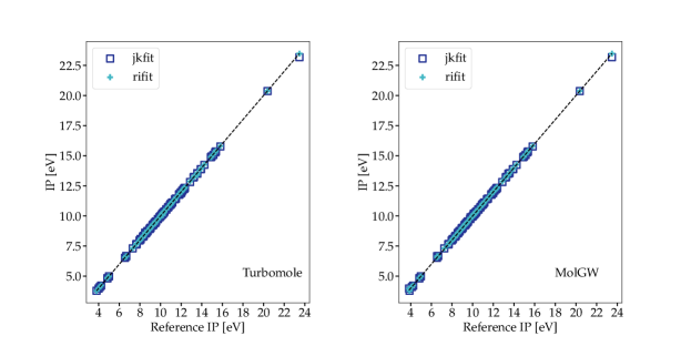
Figure 2: Comparison between the $G_{0}W_{0}$@PBE vertical ionization potentials computed with the current implementation and two other codes. Results from Turbomole and MolGW were obtained from the GW100 GitHub repository ⁷⁰ and correspond to the entries “TM v7.0 def2-QZVP RIK” and “Mv2.A def2-QZVP cc-pVQZ-RI (first peak)”. All values in eV.

Similar to the ionization potential plots, Figure 3 shows correlation plots for the computed vertical electron affinities. The outliers seen in Figure 3 correspond to the xenon atom in the Turbomole plot, and to the fluorine dimer in the MolGW plot. Interestingly, Turbomole and MolGW also differ between each other in these two cases. The MAEs worsen to 58 meV, 66 meV, and 73 meV, for JKFIT, RIFIT and MolGW, respectively.

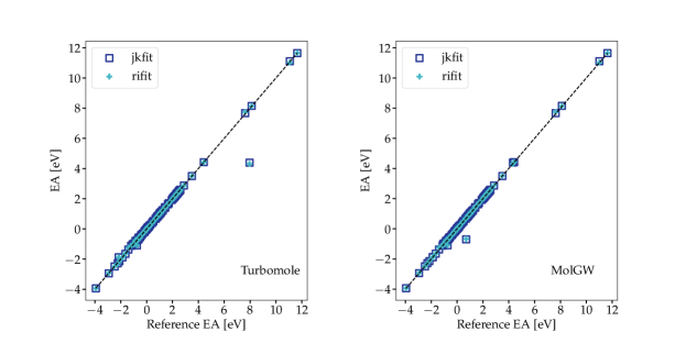
Figure 3: Comparison between the $G_{0}W_{0}$@PBE vertical electron affinities computed with the current implementation and two other codes. Results from Turbomole were taken from Ref. ⁴⁹. MolGW results were obtained from the GW100 GitHub repository ⁷⁰ and correspond to the entry “Mv2.B_def2-QZVP_auto_firstpeak”. All values in eV.

4.2 Core Spectra

The accuracy of the core-level was assessed using the CORE65 benchmark set from Golze et al. ⁵⁰. The CORE65 set contains 32 small inorganic and organic molecules with up to 14 atoms. We present comparisons to the non-relativistic results at the ev$GW_{0}$@PBE, $G_{0}W_{0}$@PBEh (see Supporting Information of Ref. 50), $G_{0}W_{0}$@PBE0, and ev$GW$@PBE0 levels of theory. All calculations used the cc-pvtz basis set and the JKFIT auxiliary basis. Here, PBEh ⁷³ refers to the hybrid functional with 45% Hartree-Fock (HF) exchange, and PBE0 ^{74, 75} to the functional with 25% HF exchange. Figures 4 and 5 show correlation plots for the aforementioned cases (see Supporting Information for individual results.)

The correlation shown for the results obtained using the PBE GGA functional is not close to linearity. This might be explained by the difficulty to find the exact same solution along the whole ev$GW_{0}$ self-consistent cycle between the two different solvers, as there are many very close solutions for the quasiparticle equations of such states^{53, 50}. In fact, our experience indicates that small energy differences ($\sim\mu$ eV) might lead our own solver to different solutions, and that these differences sometimes disappear during the ev$GW_{0}$ and ev$G_{0}W_{0}$ cycles. Nevertheless, the perfect correlation seen in the PBEh core results, as well as the very good agreement in the valence region, reassures us about the soundness of our implementation. The large fraction of HF exchange in the hybrid PBEh functional facilitates the identification of a single solution for each quasiparticle equation ^{53, 50}, leading to the expected match between codes.

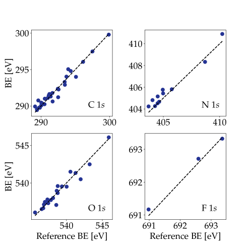
Figure 4: Correlation plot of the CORE65 ev$GW_{0}$@PBE/cc-pvtz binding energies obtained with the current implementation and from Ref. 50. The dashed lines indicate an exact match.

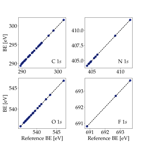
Figure 5: Correlation plot of the CORE65 $G_{0}W_{0}$@PBEh/cc-pvtz binding energies obtained with the current implementation and from Ref. 50. The dashed lines indicate an exact match.

Including 25% HF exchange, as in the PBE0 functional, does not completely resolve the multiple solution issues in the core region, but it does help to reduce the number of tightly clustered peaks. Another drawback of using a low percentage of HF exchange is that the one-shot $G_{0}W_{0}$ binding energies are still not good enough to avoid doing the more expensive ev$GW$ procedure (see Supporting Information), while the SCF step is as expensive as any other hybrid functional with larger fraction of HF exchange.

4.2.1 ESCA Molecule

Ethyl trifluoroacetate, also known as the ESCA molecule ⁷⁶, shows extreme chemical shifts in its carbon 1s (C 1s) binding energies and has been an important reference system since the dawn of photoelectron spectroscopy ⁷⁷. Previous computational studies involving the C 1s binding energies of the ESCA molecule have been performed using the $\Delta$SCF method ^{77, 78, 79, 80, 81}, but we could not find any core-level $GW$ studies reported for this molecule.

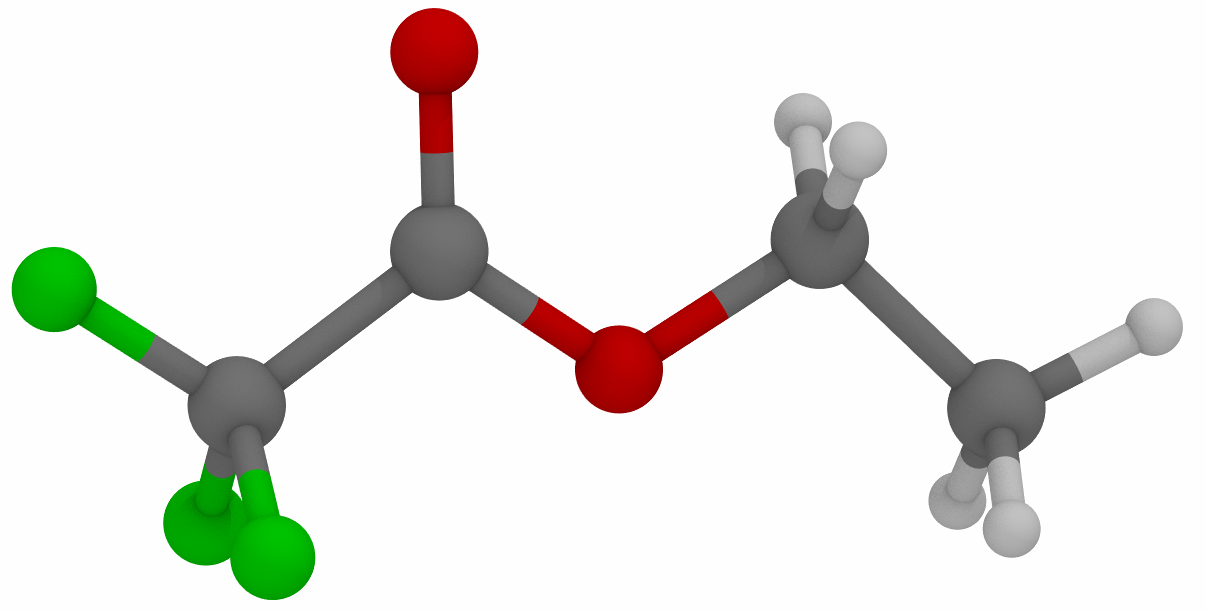
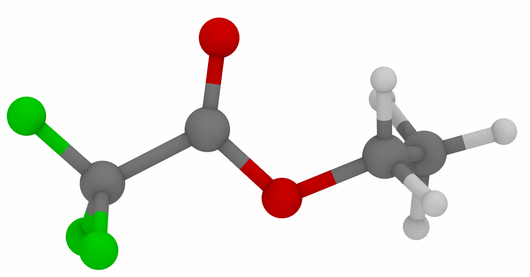
Figure 6: Ethyl trifluoroacetate in the anti-anti conformation (left) and anti-gauche conformation (right).

Table 1: Core-level binding energies of ethyl trifluoroacetate. Experimental results with respect to the vacuum level ⁷⁷. All values in eV.

C 1s peak	Experimental	ev$GW_{0}$	ev$GW_{0}$	ev$GW_{0}$	$G_{0}W_{0}$
		PBE	r2SCAN-L	r2SCAN	PBEh
CH3	291.47	289.03	290.62	291.79	291.46
CH2	293.19	291.70	292.87	293.48	293.42
CO2	295.80	293.95	295.24	296.23	296.43
CF3	298.93	297.48	298.55	299.41	299.64

Table 1 shows the absolute binding energies of the four C 1s states of the ESCA molecule. The experimental results were taken from the high-resolution photoelectron spectrum of Travnikova and cols.⁷⁷ The computed binding energies are weighted averages of the two conformations found in a gas-phase electron diffraction spectrum⁸² and shown in Figure 6.

All calculations used the experimental geometries, the pcSseg-3 quadruple-$\zeta$ basis set from Jensen⁸³ and the def2-universal-jkfit auxiliary basis set. A larger auxiliary basis set adapted to the pcSseg-3 basis using an automatic generator⁸⁴ does not change the quality of the results.

Previously, Fouda and Besley found that the pcSseg-$n$ family converges faster to the basis set limit in DFT calculations of core-electron spectroscopies.⁸⁵ We also found that the pcSseg-$n$ family describes both core and valence ionizations more uniformly than the very recent ccX-$n$Z family⁸⁶.

Four density functional approximations– PBE, r²SCAN⁸⁷, r²SCAN-L⁸⁸, and PBEh–were used to evaluate the starting points obtained from the three major exchange-correlation approximation families. No relativistic corrections were included.

Clearly, the ev$GW_{0}$@r²SCAN method yields the best overall agreement with experiment, with $G_{0}W_{0}$@PBEh results closely following. Even so, $G_{0}W_{0}$@PBEh is the method of choice because it leads to single solutions for the C 1s states. At the other end, we find the binding energies obtained with ev$GW_{0}$@r²SCAN-L and ev$GW_{0}$@PBE underbind the C 1s states but, as expected, ev$GW_{0}$@r²SCAN-L energies fall in between those of ev$GW_{0}$PBE and ev$GW_{0}$@r²SCAN, respectively. Comparisons with the $\Delta$-SCF method are presented in the Supporting Information.

5 Parallel Performance

The parallel performance and computational scaling of the CD-$G_{0}W_{0}$ implementation are assessed using water clusters with 5, 10, 15, and 20 molecules published in the Cambridge Cluster Database⁸⁹. The molecular structures of these clusters are shown in Figure 7. All calculations presented in this subsection use the def2-QZVP/def2-universal-jkfit combination of orbital and auxiliary basis sets without exploiting molecular symmetry.

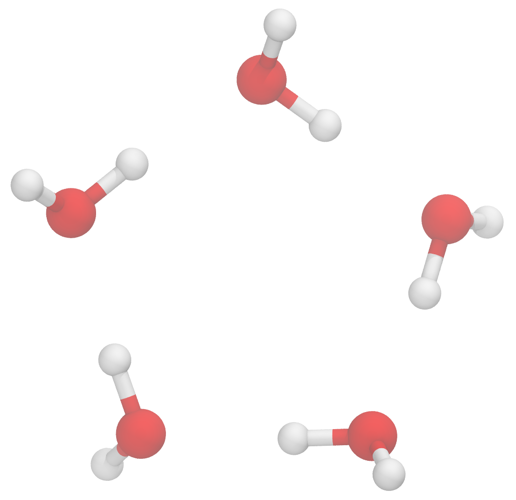
(a) (H2O)_5

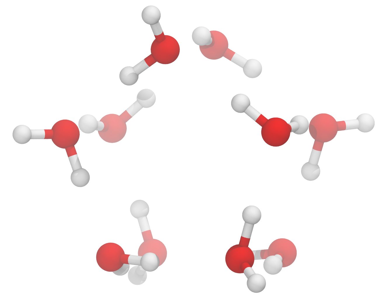
(b) (H2O)10

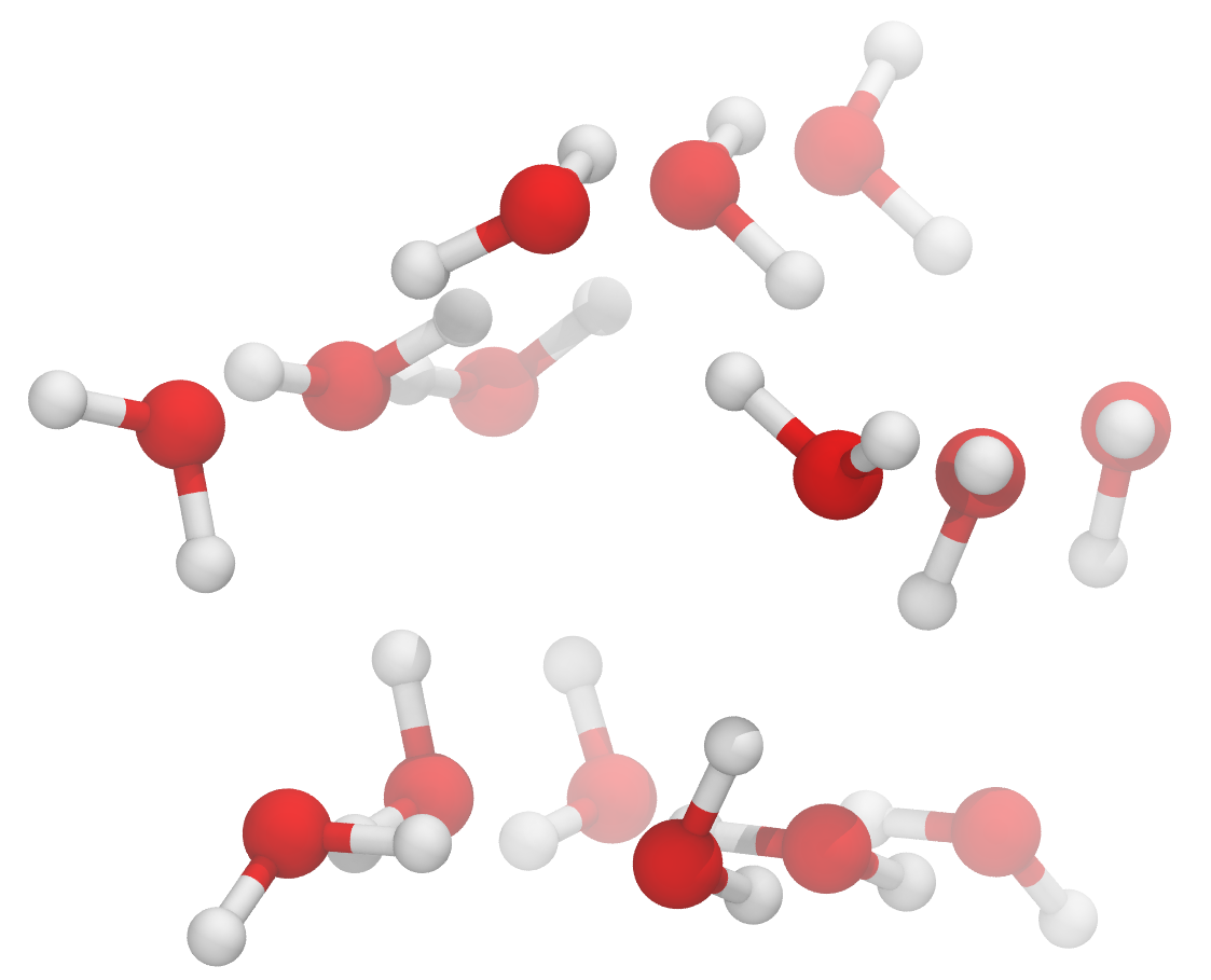
(c) (H2O)15

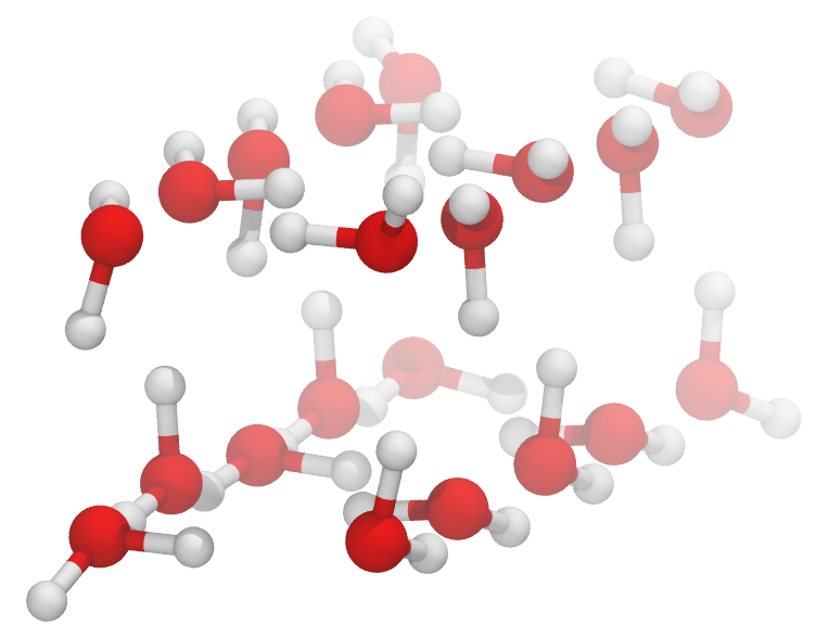
(d) (H2O)_20

Figure 7: Water cluster structures used to evaluate the computational performance of the CD-$G_{0}W_{0}$ method.

Each computational node used consists of 2 18-core sockets for a total of 36 Intel Xeon Gold 6254 cores per node with up to 384 GB of memory. However, we used a maximum of 32 cores per node.

The stacked bars in Figure 8 show the wall clock time, in seconds, needed to obtain the $G_{0}W_{0}$@PBE energies of the 5 highest occupied states of (H2O)20. Each bar is divided in four sections in order to reflect the time spent in the most demanding parts of the CD-$G_{0}W_{0}$ implementation. These tasks are 1) ERIs computation, 2) the exchange-correlation matrix elements, 3) the screened-Coulomb matrix elements on the imaginary grid $W(i\omega)$, and 4) the computation of the residue term $R_{nn}(\omega)$. Figure 8 also shows three categories per processor count, that depend on the number of OpenMP threads used per MPI rank. There are several things to mention about Figure 8. First, the ERIs and $V_{xc}$ tasks make little use of OpenMP parallelization, thus the their relative times become larger as the number of OpenMP threads increases. In contrast, both $W(i\omega)$ and $R_{nn}(\omega)$ benefit from the OpenMP parallelization. The overall result is, in general, a lower execution time for the hybrid OpenMP+MPI approach. It is also worth noting that both $W(i\omega)$ and $R_{nn}(\omega)$ tasks have roughly the same computational demand when a few valence energies are sought. This is the expected behavior since both tasks have the same $\mathcal{O}(N^{4})$ asymptotic scaling for valence states. However, the computation of core energies dramatically shift the computational burden to $R_{nn}(\omega)$, as this task has an $\mathcal{O}(N^{5})$ scaling for a core level. As a result, the overall scaling of CD-$G_{0}W_{0}$ can be as high as $N_{core}N_{vir}N_{occ}^{2}N_{aux}^{2}$ when all $N_{core}$ energies are computed.

The use of the MINRES solver changes the worst scaling to $N_{core}N_{vir}N_{occ}^{2}N_{aux}$. MINRES is therefore an important tool that contributes to the efficiency of the code. Unfortunately, MINRES can sometimes converge rather slowly. For such cases, the Bunch-Kaufman $LDL^{T}$ factorization might be more efficient. Our benchmarks showed that O $2s$ states are problematic for MINRES, and take most of the total $G_{0}W_{0}$ time. Switching to the $LDL^{T}$ factorization mildly improves the situation, but the observed scaling still comes in between $N^{5}$ and $N^{6}$ when the full spectrum is computed.

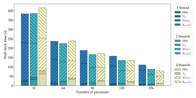
Figure 8: Wall clock time, in seconds, needed to obtain the 5 highest occupied states of the (H2O)20 cluster with the $G_{0}W_{0}$@PBE method.

This scaling can be inferred from Figure 9, which shows the wall clock times needed to obtain all the occupied spectrum of the water clusters. The execution time increases about 38 times going from (H2O)10 to (H2O)20, which implies an $N^{5.25}$ scaling. Figure 9 also shows that the scalability of the code is greatly enhanced by using the hybrid OpenMP+MPI parallelization.

As noted previously, O $2s$ states mostly determine the overall efficiency of the code in this benchmark. The use of the $LDL^{T}$ factorization carries with it both a computation and a communication penalty as compared to MINRES. We do not have a parallel $LDL^{T}$ factorization at hand to resolve this bottleneck. Still, substituting it with a parallel $LU$ factorization does not show a computational advantage for these system sizes.

Several optimized BLAS libraries do have threaded versions of the $LDL^{T}$ factorization. As a consequence, the hybrid OpenMP+MPI is generally the method of choice since it reduces both the internode communication and the time spent factorizing $\left[\mathbf{1}-\bm{\Pi}(\epsilon_{m}-\omega)\right]^{-1}$.

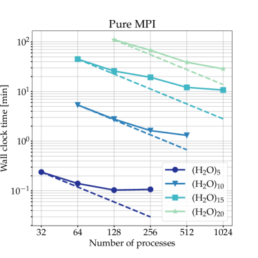
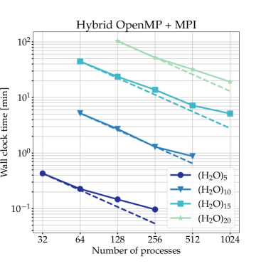
Figure 9: Scaling test with respect to the total number of processes using $G_{0}W_{0}$@PBEh to obtain the full occupied spectrum of (H2O)20. Four OpenMP threads were used for the hybrid approach and the dashed lines indicate ideal parallelization with respect to the 32-core case.

The performance of the spectral decomposition implementation hinges on the performance of the diagonalizer used. We have linked our code to the very efficient ELPA library ^{90, 91} version 2020.11.001 and used the 2-stage solver with the AVX-512 kernel ⁹². The CD-$GW$ implementation turned out to be always faster than the spectral decomposition when a few valence energies are requested. On the other hand, calculations requiring the full occupied spectrum can be faster with the spectral decomposition method up to a certain system size. The crossing point occurs at around 15 water molecules when PBE is used as the starting point, and at around 10 water molecules for PBEh. An additional disadvantage of the spectral decomposition implementation, besides its unfavorable $\mathcal{O}(N^{6})$ scaling, is that the memory scales as $2N_{occ}^{2}N_{vir}^{2}$. More often than not, the lack of memory impedes the use of the spectral decomposition method.

6 Summary

We have presented and validated a scalable and efficient all-electron $GW$ implementation using Gaussian atomic orbitals to study the valence and core ionization spectroscopies of molecular systems. Our implementation is based on the software infrastructure of the open-source NWChem quantum chemistry package. Specifically, we have implemented the spectral decomposition and contour deformation approaches using the robust variational fitting (RVF) approximation to the four-center electron repulsion integrals. The spectral decomposition approach is linked to the ELPA library for fast eigendecomposition of the Casida matrix, while the contour deformation approach uses the MINRES solver to obtain the action of the inverse dielectric matrices on any given vector. The former approach allows the fast computation of core-level spectroscopy in small molecules with up to 40 atoms, while the latter allows the computation of ionization spectra of molecules with a few hundreds of atoms in reasonable amounts of time.

To validate the accuracy of our implementation, extensive benchmark tests using the GW100 and CORE65 datasets and computations of the carbon 1s binding energy of the well-studied ethyl trifluoroacetate or ESCA molecule were performed. For the ESCA molecule, we compared the $GW$ predictions of the carbon 1s binding energy using four density functional approximations with experiment.

As a next step of the software development process, we plan to extract our $GW$ implementation to form a stand-alone domain specific library so that it can be interfaced with any Gaussian basis set based molecular DFT code. The interface will require as input from the DFT code the molecular orbitals and eigenvalue; this can be accomplished by using a variety of data formats (for example, the Molden format⁹³).

Extensions to compute neutral excitation spectra based on the BSE formalism are also under development within this framework.

The authors acknowledge funding from the Center for Scalable and Predictive methods for Excitation and Correlated phenomena (SPEC), which is funded by the U.S. Department of Energy (DOE), Office of Science, Office of Basic Energy Sciences, the Division of Chemical Sciences, Geosciences, and Biosciences. This research also benefited from computational resources provided by EMSL, a DOE Office of Science User Facility sponsored by the Office of Biological and Environmental Research and located at the Pacific Northwest National Laboratory (PNNL). PNNL is operated by Battelle Memorial Institute for the United States Department of Energy under DOE contract number DE-AC05-76RL1830. This research used resources of the National Energy Research Scientific Computing Center (NERSC), a U.S. Department of Energy Office of Science User Facility located at Lawrence Berkeley National Laboratory, operated under Contract No. DE-AC02-05CH11231.

• CORE65 benchmark results at the nonrelativistic ev$GW_{0}$@PBE, $G_{0}W_{0}$@PBEh, $G_{0}W_{0}$@PBE0, and ev$GW_{0}$@PBE0 levels.

• GW100 results for vertical ionization potentials and electron affinities at the $G_{0}W_{0}$@PBE level.

• Comparison of core-level binding energies for ethyl-trifluoroacetate using $\Delta$-HF, $\Delta$-PBEh, and $G_{0}W_{0}$@PBEh.

References

- Szabo and Ostlund 1996 Szabo, A.; Ostlund, N. Modern Quantum Chemistry: Introduction to Advanced Electronic Structure Theory; Dover Publications, Mineola, NY, 1996
- Fetter and Walecka 2003 Fetter, A. L.; Walecka, J. D. Quantum Theory of Many-Particle Systems; Dover Publications, Mineola, NY, 2003
- Shavitt and Bartlett 2009 Shavitt, I.; Bartlett, R. J. Many-body methods in chemistry and physics: MBPT and coupled-cluster theory; Cambridge University Press, 2009
- Hedin 1965 Hedin, L. New method for calculating the one-particle Green’s function with application to the electron-gas problem. Physical Review 1965, 139, A796
- Aryasetiawan and Gunnarsson 1998 Aryasetiawan, F.; Gunnarsson, O. The GW method. Reports on Progress in Physics 1998, 61, 237
- Onida et al. 2002 Onida, G.; Reining, L.; Rubio, A. Electronic excitations: density-functional versus many-body Green’s-function approaches. Reviews of modern physics 2002, 74, 601
- Leng et al. 2016 Leng, X.; Jin, F.; Wei, M.; Ma, Y. GW method and Bethe-Salpeter equation for calculating electronic excitations. Wiley Interdisciplinary Reviews: Computational Molecular Science 2016, 6, 532–550
- Cancés et al. 2016 Cancés, E.; Gontier, D.; Stoltz, G. A mathematical analysis of the GW0 method for computing electronic excited energies of molecules. Reviews in Mathematical Physics 2016, 28, 1650008
- Reining 2018 Reining, L. The GW approximation: content, successes and limitations. Wiley Interdisciplinary Reviews: Computational Molecular Science 2018, 8, e1344
- Golze et al. 2019 Golze, D.; Dvorak, M.; Rinke, P. The GW compendium: A practical guide to theoretical photoemission spectroscopy. Frontiers in chemistry 2019, 7, 377
- Salpeter and Bethe 1951 Salpeter, E. E.; Bethe, H. A. A relativistic equation for bound-state problems. Physical Review 1951, 84, 1232
- Faleev et al. 2004 Faleev, S. V.; Van Schilfgaarde, M.; Kotani, T. All-Electron Self-Consistent G W Approximation: Application to Si, MnO, and NiO. Physical review letters 2004, 93, 126406
- Stan et al. 2009 Stan, A.; Dahlen, N. E.; Van Leeuwen, R. Levels of self-consistency in the GW approximation. The Journal of chemical physics 2009, 130, 114105
- Caruso et al. 2012 Caruso, F.; Rinke, P.; Ren, X.; Scheffler, M.; Rubio, A. Unified description of ground and excited states of finite systems: The self-consistent G W approach. Physical Review B 2012, 86, 081102
- van Setten et al. 2013 van Setten, M. J.; Weigend, F.; Evers, F. The -method for quantum chemistry applications: Theory and Implementation. Journal of Chemical Theory and Computation 2013, 9, 232–246
- Kaplan et al. 2016 Kaplan, F.; Harding, M.; Seiler, C.; Weigend, F.; Evers, F.; van Setten, M. J. Quasi-particle self-consistent calculations. Journal of Chemical Theory and Computation 2016, 12, 2528–2541
- Holzer and Klopper 2019 Holzer, C.; Klopper, W. Ionized, electron-attached, and excited states of molecular systems with spin-orbit coupling: Two-component and Bethe-Salpeter implementations. The Journal of Chemical Physics 2019, 150, 204116
- Balasubramani et al. 2020 Balasubramani, S. G.; Chen, G. P.; Coriani, S.; Diedenhofen, M.; Frank, M. S.; Franzke, Y. J.; Furche, F.; Grotjahn, R.; Harding, M. E.; Hättig, C. et al. TURBOMOLE: Modular program suite for ab initio quantum-chemical and condensed-matter simulations. The Journal of Chemical Physics 2020, 152, 184107
- Caruso et al. 2013 Caruso, F.; Rinke, P.; Ren, X.; Rubio, A.; Scheffler, M. Self-consistent : All-electron implementation with localized basis functions. Physical Review B 2013, 88, 075105
- Wilhelm et al. 2018 Wilhelm, J.; Golze, D.; Talirz, L.; Hutter, J.; Pignedoli, C. A. Toward calculations on thousands of atoms. The Journal of Physical Chemistry Letters 2018, 9, 306–312
- Kühne et al. 2020 Kühne, T. D.; Iannuzzi, M.; Del Ben, M.; Rybkin, V. V.; Seewald, P.; Stein, F.; Laino, T.; Khaliullin, R. Z.; Schütt, O.; Schiffmann, F. et al. CP2K: An electronic structure and molecular dynamics software package - Quickstep: Efficient and accurate electronic structure calculations. The Journal of Chemical Physics 2020, 152, 194103
- Förster and Visscher 2020 Förster, A.; Visscher, L. Low-order scaling by pair atomic density fitting. Journal of Chemical Theory and Computation 2020, 16, 7381–7399
- Bruneval et al. 2016 Bruneval, F.; Rangel, T.; Hamed, S. M.; Shao, M.; Yang, C.; Neaton, J. B. molgw 1: Many-body perturbation theory software for atoms, molecules, and clusters. Computer Physics Communications 2016, 208, 149–161
- Deslippe et al. 2012 Deslippe, J.; Samsonidze, G.; Strubbe, D. A.; Jain, M.; Cohen, M. L.; Louie, S. G. BerkeleyGW: A massively parallel computer package for the calculation of the quasiparticle and optical properties of materials and nanostructures. Computer Physics Communications 2012, 183, 1269
- Gianozzi et al. 2009 Gianozzi, P.; Baroni, S.; Bonini, N.; Calandra, M.; Car, R.; Cavazzoni, C.; Ceresoli, D.; Chiarotti, G. L.; Cococcioni, M.; Dabo, I. et al. Quantum ESPRESSO: a modular and open-source software project for quantum simulations of materials. Journal of Physics: Condensed Matter 2009, 21, 395502
- Gianozzi et al. 2017 Gianozzi, P.; Andreussi, O.; Brumme, T.; Bunau, O.; Buongiorno Nardelli, M.; Calandra, M.; Car, R.; Cavazzoni, C.; Ceresoli, D.; Cococcioni, M. et al. Advanced capabilities for materials modellin with Quantum ESPRESSO. Journal of Physics: Condensed Matter 2017, 29, 465901
- Umari et al. 2009 Umari, P.; Stenuit, G.; Baroni, S. Optimal representation of the polarization propagator for large-scale calculations. Physical Review B 2009, 79, 201104(R)
- Umari et al. 2010 Umari, P.; Stenuit, G.; Baroni, S. GW quasiparticle spectra from occupied states only. Physical Review B 2010, 81, 115104
- Gonze et al. 2020 Gonze, X.; Amadon, B.; Antonius, G.; Arnardi, F.; Baguet, L.; Beuken, J.-M.; Bieder, J.; Bottin, F.; Bouchet, J.; Bousquet, E. et al. The Abinit project: Impact, environment and recent developments. Computer Physics Communications 2020, 248, 107042
- Kresse and Hafner 1993 Kresse, G.; Hafner, J. Ab initio molecular dynamics for liquid metals. Physical Review B 1993, 47, 558(R)
- Kresse and Hafner 1994 Kresse, G.; Hafner, J. Ab initio molecular-dynamics simulation of liquid-metal-amorphous-semiconductor transition in germanium. Physical Review B 1994, 49, 14251
- Kresse and Furthmüller 1996 Kresse, G.; Furthmüller, J. Efficiency of ab-initio total energy calculations for metals and semiconductors using a plane-wave basis set. Computational Materials Science 1996, 6, 15–50
- Kresse and Furthmüller 1996 Kresse, G.; Furthmüller, J. Efficient iterative schemes for ab initio total-energy calculations using a plane-wave basis set. Physical Review B 1996, 54, 11169
- Marini et al. 2009 Marini, A.; Hogan, C.; GRüning, M.; Varsano, D. yambo: An ab initio tool for excited state calculations. Computer Physics Communications 2009, 180, 1392
- Sangalli et al. 2019 Sangalli, D.; Ferretti, A.; Miranda, H.; Attaccalite, C.; Marri, I.; Cannuccia, E.; Melo, P.; Marsili, M.; Paleari, F.; Marrazzo, A. Many-body perturbation theory calculations using the yambo code. Journal of Physics: Condensed Matter 2019, 31, 325902
- Govoni and Galli 2015 Govoni, M.; Galli, G. Large scale GW calculations. Journal of Chemical Theory and Computation 2015, 11, 2680–2696
- 37 The Elk Code. http://elk.sourceforge.net/
- Sun et al. 2018 Sun, Q.; Berkelbach, T. C.; Blunt, N. S.; Booth, G. H.; Guo, S.; Li, Z.; Liu, J.; McClain, J. D.; Sayfutyarova, E. R.; Sharma, S. et al. PySCF: the Python-based simulations of chemistry framework. WIREs Computational Molecular Science 2018, 8, e1340
- Sun et al. 2020 Sun, Q.; Zhang, X.; Banerjee, S.; Bao, P.; Barbry, M.; Blunt, N. S.; Bogdanov, N. A.; Booth, G. H.; Chen, J.; Cui, Z.-H. et al. Recent developments in the PySCF program package. The Journal of Chemical Physics 2020, 153, 024109
- Mortensen et al. 2005 Mortensen, J. J.; Hansen, L. B.; Jacobsen, K. W. Real-space grid implementation of the projector augmented wave method. Physical Review B 2005, 71, 035109
- Enkovaara et al. 2010 Enkovaara, J.; Rostgaard, C.; Mortensen, J. J.; Chen, J.; Dułak, M.; Ferrighi, L.; Gavnholt, J.; Glinsvad, C.; Haikola, V.; Hansen, H. A. et al. Electronic structure calculations with GPAW: a real-space implementation of the projector augmented wave method. Journal of Physics: Condensed Matter 2010, 22, 253202
- Hüser et al. 2013 Hüser, F.; Olsen, T.; Thygesen, K. S. Quasiparticle GW calculations for solids, molecules, and two-dimensional materials. Physical Review B 2013, 87, 235132
- 43 Blaha, P.; Schwarz, K.; Tran, F.; Laskowski, R.; Madsen, G. K. H.; Marks, L. D. WIEN2k: An APW+lo program for calculating the properties of solids. The Journal of Chemical Physics 152, 074101
- Jiang et al. 2013 Jiang, H.; Gómez-Abal, R. I.; Li, X.-Z.; Meisenbichler, C.; Ambrosch-Draxl, C.; Scheffler, M. FHI-gap: A code based on the all-electron augmented plane wave method. Computer Physics Communications 2013, 184, 348–366
- Jianh and Blaha 2016 Jianh, H.; Blaha, P. with linearized augmented plane waves extended by high-energy local orbitals. Physical Review B 2016, 93, 115203
- Pashov et al. 2020 Pashov, D.; Acharya, S.; Lambrecht, W. R. L.; Jackson, J.; Belaschenko, K. D.; Chantis, A.; Jamet, F.; van Schilfgaarde, M. Questaal, A package of electronic structure methods based on the linear muffin-tin orbital technique. Computer Physics Communications 2020, 249, 107065
- Friedrich et al. 2010 Friedrich, C.; Blügel, S.; Schindlmayr, A. Efficient implementation of the approximation within the all-electron FLAPW method. Physical Review B 2010, 81, 125102
- Aprà et al. 2020 Aprà, E.; Bylaska, E. J.; de Jong, W. A.; Govind, N.; Kowalski, K.; Straatsma, T. P.; Valiev, M.; van Dam, H. J. J.; Alexeev, Y.; Anchell, J. et al. NWChem: Past, present, and future. The Journal of Chemical Physics 2020, 152, 184102
- van Setten et al. 2015 van Setten, M. J.; Caruso, F.; Sharifzadeh, S.; Ren, X.; Scheffler, M.; Liu, F.; Lischner, J.; Lin, L.; Deslippe, J. R.; Louie, S. G. et al. 100: Benchmarking for molecular systems. Journal of Chemical Theory and Computation 2015, 11, 5665
- Golze et al. 2020 Golze, D.; Keller, L.; Rinke, P. Accurate absolute and relative core-level binding energies from . Journal of Physical Chemistry Letters 2020, 11, 1840
- Adler 1962 Adler, S. L. Quantum theory of the dielectric constant in real solids. Physical Review 1962, 126, 413
- Wiser 1963 Wiser, N. Dielectric constant with local field effect included. Physical Review 1963, 129, 62
- Golze et al. 2018 Golze, D.; Wilhelm, J.; van Setten, M. J.; Rinke, P. Core-level binding energies from : An efficient full-frequency approach within a localized basis. Journal of Chemical Theory and Computation 2018, 14, 4856–4869
- Whitten 1973 Whitten, J. L. Coulombic potential energy integrals and approximations. The Journal of Chemical Physics 1973, 58, 4496
- Dunlap et al. 1979 Dunlap, B. I.; Connolly, J. W. D.; Sabin, J. R. On some approximations in applications of theory. The Journal of Chemical Physics 1979, 71, 3396
- Dunlap 2000 Dunlap, B. I. Robust and variational fitting: Removing the four-center integrals from center stage in quantum chemistry. Journal of Molecular Structure: THEOCHEM 2000, 529, 37–40
- Vahtras et al. 1993 Vahtras, O.; Almlöf, J.; Feyereisen, M. W. Integral approximations for LCAO-SCF calculations. Chemical Physics Letters 1993, 213, 514–518
- Wirz et al. 2017 Wirz, L. N.; Reine, S. S.; Pedersen, T. B. On resolution-of-the-identity electron repulsion integral approximations and variational stability. Journal of Chemical Theory and Computation 2017, 13, 4897–4906
- Wilhelm et al. 2021 Wilhelm, J.; Seewald, P.; Golze, D. Low-scaling with benchmark accuracy and application to phosphorene nanosheets. Journal of Chemical Theory and Computation 2021, 17, 1662–1677
- Merlot et al. 2013 Merlot, P.; Kjærgaard, T.; Helgaker, T.; Lindh, R.; Aquilante, F.; Reine, S.; Pedersen, T. B. Attractive electron-electron interactions within robust local fitting approximations. Journal of Computational Chemistry 2013, 34, 1486–1496
- Bau 1996 Treatment of electronic excitations within the adiabatic approximation of time dependent density functional theory. Chemical Physics Letters 1996, 256, 454–464
- Ren et al. 2012 Ren, X.; Rinke, P.; Blum, V.; Wieferink, J.; Tkatchenko, A.; Sanfilippo, A.; Reuter, K.; Scheffler, M. Resolution-of-the-identity approach to Hartree-Fock, hybrid density functionals, RPA, MP2 and with numeric atom-centered orbital basis functions. New Journal of Physics 2012, 14, 053020
- Gustavson et al. 2010 Gustavson, F. G.; Waśniewski, J.; Dongarra, J. J.; Langou, J. Rectangular full packed format for Cholesky’s algorithm: factorization, solution, and inversion. ACM Transactions on mathematical software 2010, 37, 1–21
- Anderson et al. 1999 Anderson, E.; Bai, Z.; Bischof, C.; Blackford, S.; Demmel, J.; Dongarra, J.; Du Croz, J.; Greenbaum, A.; Hammarling, S.; McKenney, A. et al. LAPACK Users’ Guide, 3rd ed.; Society for Industrial and Applied Mathematics: Philadelphia, PA, 1999
- Paige and Saunders 1975 Paige, C. C.; Saunders, M. A. Solution of sparse indefinite systems of linear equations. SIAM Journal of Numerical Analysis 1975, 12, 617–629
- Eirola and Nevanlinna 1989 Eirola, T.; Nevanlinna, O. Accelerating with rank-one updates. Linear Algebra and its Applications 1989, 121, 511–520
- Mejía-Rodríguez et al. 2015 Mejía-Rodríguez, D.; Delgado Venegas, R. I.; Calaminici, P.; Köster, A. Robust and efficient auxiliary density perturbation theory. Journal of Chemical Theory and Computation 2015, 11, 1493–1500
- Bunch and Kaufman 1977 Bunch, J. R.; Kaufman, L. Some stable methods for calculating inertia and solving symmetric linear systems. Mathematics of Computation 1977, 31, 163–179
- Nelder and Mead 1965 Nelder, J. A.; Mead, R. A simplex method for function minimization. Computer Journal 1965, 7, 308–313
- 70 van Setten, M. GW100. https://www.github.com/setten/GW100, [Online; accessed 09-March-2021]
- Weigend 2008 Weigend, F. Hartree-Fock exchange fitting basis for H to Rn. Journal of Computational Chemistry 2008, 29, 167–175
- Hättig 2005 Hättig, C. Optimization of auxiliary basis sets for RI-MP2 and RI-CC2 calculations: Core-valence and quintuple- basis sets for H to Ar and QZVPP basis sets for Li to Kr. Physical Chemistry Chemical Physics 2005, 7, 59–66
- Atalla et al. 2013 Atalla, V.; Yoon, M.; Caruso, F.; Rinke, P.; Scheffler, M. Hybrid density functional theory meets quasiparticle calculations: A consistent electronic structure approach. Physical Review B 2013, 88, 165122
- Perdew et al. 1996 Perdew, J. P.; Ernzerhof, M.; Burke, K. Rationale for mixing exact exchange with density functional approximations. The Journal of Chemical Physics 1996, 105, 9982
- Adamo and Barone 1999 Adamo, C.; Barone, V. Toward reliable density functional methods without adjustable parameters: The PBE0 model. The Journal of Chemical Physics 1999, 110, 6158
- Siegbahn et al. 1967 Siegbahn, K.; Nordling, C.; Fahlman, A.; Nordberg, R.; Hamrin, K.; Hedman, J.; Johansson, G.; Bergmark, T.; Karlsson, S.-E.; Lindgren, I. et al. ESCA, Atomic Molecular and Solid State Structure Studied by Means of Electron Spectroscopy; Almqvist and Wiksells: Uppsala, Sweden, 1967
- Travnikova et al. 2012 Travnikova, O.; Børve, K. J.; Patanen, M.; Söderström, J.; Miron, C.; Sæthre, L. J.; Mårtensson, N.; Svensson, S. The ESCA molecule–Historical remarks and new results. Journal of Electron Spectroscopy and Related Phenomena 2012, 185, 191–197
- Van den Bossche et al. 2014 Van den Bossche, M.; Martin, N. M.; Gustafson, J.; Hakanoglu, C.; Weaver, J. F.; Lundgren, E.; Grönbeck, H. Effects of non-local exchange on core level shifts for gas-phase and adbosrbed molecules. The Journal of Chemical Physics 2014, 141, 034706
- Delesma et al. 2017 Delesma, F. A.; Van Den Bossche, M.; Grönbeck, H.; Calaminici, P.; Köster, A. M.; Pettersson, L. G. M. A chemical view x-ray photoelectron spectroscopy: the ESCA molecule and surface-to-bulk XPS shifts. ChemPhysChem 2017, 19, 169–174
- Travnikova et al. 2019 Travnikova, O.; Patanen, M.; Söderström, J.; Lindbald, A.; Kas, J. J.; Vila, F. D.; Céolin, D.; Marchenko, T.; Goldstejn, G.; Guillemin, R. et al. Energy-dependent relative cross-sections in carbon 1s photoionization: Separation of direct shake and inelestic scattering effects in single molecules. The Journal of Physical Chemistry A 2019, 123, 7619–7636
- Klein et al. 2021 Klein, B. P.; Hall, S. J.; Maurer, R. J. The nuts and bolts of core-hole constrained ab initio simulation for -shell x-ray photoemission and absorption spectra. Journal of Physics: Condensed Matter 2021, 33, 154005
- Defonsi Lestard et al. 2010 Defonsi Lestard, M. E.; Tuttolomondo, M. E.; Wann, D. A.; Robertson, H. E.; Rankin, D. W.; Altabef, A. B. Experimental and theoretical structure and vibrational analysis of ethyl trifluoroacetate, \ceCF3CO2CH2CH3. Journal of Raman Spectroscopy 2010, 41, 1357–1368
- Jensen 2008 Jensen, F. Basis set convergence of nuclear magnetic shielding constants calculated by density functional methods. Journal of Chemical Theory and Computation 2008, 4, 719–727
- Stoychev et al. 2017 Stoychev, G. L.; Auer, A. A.; Neese, F. Automatic generation of auxiliary basis sets. Journal of Chemical Theory and Computation 2017, 13, 554–562
- Fouda and Besley 2018 Fouda, A. E. A.; Besley, N. A. Assessment of basis sets for density functional theory-based calculations of core-electron spectroscopies. Theoretical Chemistry Accounts 2018, 137, 6
- Ambroise et al. 2021 Ambroise, M. A.; Dreuw, A.; Jensen, F. Probing basis set requirements for calculating core ionization and core excitation spectra using correlated wave function methods. Journal of Chemical Theory and Computation 2021, 17, 2832–2842
- Furness et al. 2020 Furness, J. W.; Kaplan, A. D.; Ning, J.; Perdew, J. P.; Sun, J. Accurate and numerically efficient r2SCAN meta-generalized gradient approximation. The Journal of Physical Chemistry Letters 2020, 11, 8208–8215
- Mejia-Rodriguez and Trickey 2020 Mejia-Rodriguez, D.; Trickey, S. B. Meta-GGA performance in solids at almost GGA cost. Physical Review B 2020, 102, 121109(R)
- Maheshwary et al. 2001 Maheshwary, S.; Patel, N.; Sathyamurthi, N.; Kulkarni, A. D.; Gadre, S. R. Structure and stability of water clusters \ce(H2O)_n, : An ab initio investigation. The Journal of Physical Chemistry A 2001, 105, 10525–10537
- Auckenthaler et al. 2011 Auckenthaler, T.; Blum, V.; Bungartz, H.-J.; Huckle, T.; Johanni, R.; Krämer, L.; Lang, B.; Lederer, H.; Willems, P. R. Parallel solution of partial symmetric eigenvalue problems from electronic structure calculations. Parallel Computing 2011, 37, 783–794
- Marek et al. 2014 Marek, A.; Blum, V.; Johanni, R.; Havu, V.; Lang, B.; Auckenthaler, T.; Heinecke, A.; Bungartz, H.-J.; Lederer, H. The ELPA library: scalable parallel eigenvalue solutions for electronic structure theory and computational science. Journal of Physics: Condensed Matter 2014, 26, 213201
- Kus et al. 2019 Kus, P.; Marek, A.; Koecher, S. S.; Kowalski, H.-H.; Carbogno, C.; Scheurer, C.; Reuter, K.; Scheffler, M.; Lederer, H. Optimizations of the eigenvaluesolvers in the ELPA library. Parallel Computing 2019, 85, 167–177
- Schaftenaar et al. 2017 Schaftenaar, G.; Vlieg, E.; Vriend, G. Molden 2.0: quantum chemistry meets proteins. Journal of Computer-Aided Molecular Design 2017, 31, 789–800