Designing a Location Trace Anonymization Contest

Abstract.

For a better understanding of anonymization methods for location traces, we have designed and held a location trace anonymization contest that deals with a long trace (400 events per user) and fine-grained locations (1024 regions). In our contest, each team anonymizes her original traces, and then the other teams perform privacy attacks against the anonymized traces. In other words, both defense and attack compete together, which is close to what happens in real life. Prior to our contest, we show that re-identification alone is insufficient as a privacy risk and that trace inference should be added as an additional risk. Specifically, we show an example of anonymization that is perfectly secure against re-identification and is not secure against trace inference. Based on this, our contest evaluates both the re-identification risk and trace inference risk and analyzes their relationship. Through our contest, we show several findings in a situation where both defense and attack compete together. In particular, we show that an anonymization method secure against trace inference is also secure against re-identification under the presence of appropriate pseudonymization. We also report defense and attack algorithms that won first place, and analyze the utility of anonymized traces submitted by teams in various applications such as POI recommendation and geo-data analysis.

1. Introduction

Location-based services (LBS) such as POI (Point of Interest) search, route finding, and POI recommendation (Cheng et al., 2013; Feng et al., 2015; Liu et al., 2017) have been widely used in recent years. For example, a smartphone or in-car navigation system may repeatedly send a user’s location to an LBS provider to receive services such as route finding and POI recommendation. The sequence of locations is called a location trace. With the spread of such services, a large amount of location traces are accumulating in a data center of the LBS provider. These traces can be provided to a third party to perform various geo-data analysis tasks such as mining popular POIs (Zheng et al., 2009), auto-tagging POI categories (e.g., restaurants, hotels) (Do and Gatica-Perez, 2013; Ye et al., 2011), and modeling human mobility patterns (Liu et al., 2013; Song et al., 2006).

However, the disclosure of location traces raises a serious privacy concern (on leaks of sensitive data). For example, there is a risk that the traces are used to infer sensitive social relationships (Bilogrevic et al., 2013; Eagle et al., 2009) or hospitals visited by users. Some studies have shown that even if the traces are pseudonymized, original user IDs can be re-identified with high probability (Gambs et al., 2014; Mulder et al., 2008; Murakami, 2017). This fact indicates that the pseudonymization alone is not sufficient and anonymization is necessary before providing traces to a third party. In the context of location traces, anonymization consists of location obfuscation (e.g., adding noise, generalization, and deleting some locations) and pseudonymization.

Finding an appropriate anonymization method for location traces is extremely challenging. For example, each location in a trace can be highly correlated with the other locations. Consequently, an anonymization mechanism based on differential privacy (DP) (Dwork, 2006; Dwork and Roth, 2014) might not guarantee high privacy and utility (usefulness of the anonymized data for LBS or geo-data analysis). More specifically, consider releasing location traces (Andrés et al., 2013; Meehan and Chaudhuri, 2021; Xiao and Xiong, 2015) or aggregate time-series (time-dependent population distribution) (Pyrgelis et al., 2017). It is well known that DP with a small privacy budget $\varepsilon$ (e.g., $\varepsilon=0.1$ or $1$ (Li et al., 2016)) provides strong privacy against adversaries with arbitrary background knowledge. However, DP might result in no meaningful privacy guarantees or poor utility for long traces (Andrés et al., 2013; Pyrgelis et al., 2017) (unless we limit the adversary’s background knowledge (Meehan and Chaudhuri, 2021; Xiao and Xiong, 2015)), as $\varepsilon$ in DP tends to increase with increase in the trace length. Thus, there is still no conclusive answer on how to appropriately anonymize location traces, which motivates our objective of designing a contest.

Location Trace Anonymization Contest.  To better understand anonymization methods for traces, we have designed and held a location trace anonymization contest called PWS (Privacy Workshop) Cup 2019 (PWS, 2019). Our contest has two phases: anonymization phase and privacy attack phase. In the anonymization phase, each team anonymizes her original traces. Then in the privacy attack phase, the other teams obtain the anonymized traces and perform privacy attacks against the anonymized traces. Based on this, we evaluate privacy and utility of the anonymized traces for each team. In other words, we model the problem of finding an appropriate anonymization method as a battle between a designer of the anonymization method (each team) and adversaries (the other teams). One promising feature of our contest is that both defense and attack compete together, which is close to what happens in real life.

The significance of a location trace anonymization contest is not limited to finding appropriate anonymization methods. For example, it is useful for an educational purpose – everyone can join the contest to understand the importance of anonymization (e.g., why the pseudonymization alone is not sufficient) or to improve her own anonymization skill.

However, designing a location trace anonymization contest poses great challenges. In particular, an in-depth understanding of privacy risks is crucial for finding better anonymization methods. Below, we explain this issue in more detail.

Privacy Risks.  Privacy risks have been extensively studied over the past two decades (Aggarwal and Yu, 2008; Torra, 2017). In particular, re-identification (or de-anonymization) has been acknowledged as a major risk in the privacy literature. Re-identification refers to matching anonymized data with publicly available information or auxiliary data to discover the individual to which the data belongs (Re-identification — CROS - European Commission, 2019). In the literature on location privacy, re-identification is defined as a problem of mapping anonymized or pseudonymized traces to the corresponding user IDs (Gambs et al., 2014; Mulder et al., 2008; Murakami, 2017; Shokri et al., 2011). It has been demonstrated that re-identification attacks are very effective for apparently anonymized data, such as medical records in the Group Insurance Commission (GIC) (Sweeney, 2002) and the Netflix Prize dataset (Narayanan and Shmatikov, 2008). Re-identification of data subjects is also acknowledged as a major risk in data protection laws, such as General Data Protection Regulation (GDPR) (The EU General Data Protection Regulation (2016), GDPR; Maldoff, 2016).

Attribute inference, which infers attributes of an individual, is another major privacy risk. In particular, it is known that some attributes may be inferred without re-identifying records (Torra, 2017; Garfinkel, 2015). Its famous example is an attribute inference attack against $k$-anonymity (Machanavajjhala et al., 2006). $k$-anonymity guarantees that every record is indistinguishable from at least $k-1$ other records with respect to quasi-identifiers (e.g., ZIP code and birth date). Thus, an adversary who knows only quasi-identifiers cannot re-identify a record with a probability larger than $1/k$. However, if the $k$ records have the same sensitive attribute (e.g., cancer), an adversary who knows a patient’s quasi-identifiers can infer her sensitive attribute without re-identifying her record. This attack is called the homogeneity attack and motivates the notion of $l$-diversity (Machanavajjhala et al., 2006). Similarly, Shokri et al. (Shokri et al., 2011) show that $k$-anonymity for location traces is vulnerable to attribute inference attacks, where the attribute is a location in this case.

In this paper, we provide stronger evidence that re-identification alone is not sufficient as a privacy risk – we provide an example of anonymization that is perfectly secure against re-identification and is not secure against attribute inference. Specifically, we show that the cheating anonymization (Kikuchi et al., 2016a) (or excessive anonymization (Nojima et al., 2018)), which excessively anonymizes each record, has this property.

In location traces, the cheating anonymization can be explained as follows. Consider a dataset in Figure 1. In this example, there are three users ($v_{1}$, $v_{2}$, and $v_{3}$) and four types of discrete locations ($x_{1}$, $x_{2}$, $x_{3}$, and $x_{4}$). We excessively add noise to their original traces so that obfuscated traces of users $v_{1}$, $v_{2}$, and $v_{3}$ are the same as the original traces of users $v_{2}$, $v_{3}$, and $v_{1}$, respectively. Note that this is location obfuscation rather than pseudonymization. Then we pseudonymize these traces so that pseudonyms $10001$, $10002$, and $10003$ correspond to $v_{1}$, $v_{2}$, and $v_{3}$, respectively.

Figure 1. Cheating anonymization.

This anonymization is seemingly insecure because it just shuffles the original traces in the same way as pseudonymization. However, this anonymization is secure against re-identification, unlike pseudonymization. To show this, consider an adversary who knows the original traces or any other traces highly correlated with the original traces. This adversary would re-identify $10001$, $10002$, and $10003$ as $v_{2}$, $v_{3}$, and $v_{1}$, respectively. However, $10001$, $10002$, and $10003$ actually correspond to $v_{1}$, $v_{2}$, and $v_{3}$, respectively, as explained above. Therefore, this re-identification attack fails – the re-identification rate is $\frac{0}{3}$. This is caused by the fact that we excessively obfuscate the locations so that the shuffling occurs before pseudonymization. Note that this shuffling can be viewed as a random permutation of user IDs before pseudonymization. Thus, the cheating anonymization is perfectly secure against re-identification in that the anonymized traces provide no information about user IDs; i.e., the adversary cannot find which permutation is correct.

Although the security of the cheating anonymization against re-identification is explained in (Kikuchi et al., 2016a; Nojima et al., 2018), the security of this method against attribute inference has not been explored. Therefore, prior to our contest, we evaluate the privacy of the cheating anonymization against attribute inference through experiments. Our experimental results show that the cheating anonymization is not secure against a trace inference attack (a.k.a. tracking attack (Shokri et al., 2011)), which infers the whole locations in the original traces. In other words, we show that the adversary can recover the original traces from anonymized traces without re-identifying them. Note that $k$-anonymity is not perfectly secure against re-identification unless $k$ is equal to the total number of records. In contrast, the cheating anonymization is perfectly secure against re-identification, as explained above. Thus, our experimental results strongly demonstrate that re-identification alone is insufficient as a privacy risk and that trace inference should be added as an additional risk.

Our Contest.  Based on our experimental results, our contest evaluates both the re-identification risk and trace inference risk and analyzes their relationship. In particular, since we know that the security against re-identification does not imply the security against trace inference, we pose the following question: Does the security against trace inference imply the security against re-identification? Through our contest, we show that the answer is yes under the presence of appropriate pseudonymization.

We also show other findings based on our contest. First, we explain how the best defense and attack algorithms that won first place in our contest are effective compared to existing algorithms such as (Bettini et al., 2009; Chow and Mokbel, 2011; Gedik and Liu, 2008; Gambs et al., 2014; Mulder et al., 2008; Murakami, 2017; Murakami et al., 2017; Shokri et al., 2011). Second, we show that anonymized traces submitted by teams are useful for various applications such as POI recommendation (Cheng et al., 2013; Feng et al., 2015; Liu et al., 2017) and geo-data analysis.

Our Contributions.  Our contributions are as follows:

• Through experiments, we show that there exists an algorithm perfectly secure against re-identification and not secure against trace inference.

• Based on our experimental results, we design and hold a location trace anonymization contest that evaluates both the re-identification and trace inference risks. Through our contest, we show that an anonymization method secure against trace inference is also secure against re-identification under the presence of appropriate pseudonymization. This finding is important because it provides a guideline on how to anonymize traces so that they are secure against both re-identification and attribute (trace) inference. We also report the best defense and attack algorithms in our contest and analyze their utility in various applications such as POI recommendation and geo-data analysis.

Basic Notations.  Let $\mathbb{N}$, $\mathbb{Z}_{\geq 0}$, and $\mathbb{R}$ be the set of natural numbers, non-negative integers, and real numbers, respectively. For $a\in\mathbb{N}$, let $[a]=\{1,2,\cdots,a\}$. Let $\tau\in\mathbb{N}$ be the number of teams in a contest. For $t\in[\tau]$, let $P_{t}$ be the $t$-th team. We use these notations throughout this paper.

2. Related Work

Re-identification and Attribute Inference.  Re-identification has been acknowledged as a major risk in the privacy literature and data protection laws, such as GDPR (The EU General Data Protection Regulation (2016), GDPR; Maldoff, 2016). Famous examples of re-identification attacks include Sweeney’s attack against medical records (Sweeney, 2002) and Narayanan-Shmatikov’s attack against the Netflix Prize dataset (Narayanan and Shmatikov, 2008). Re-identification has also been studied in location privacy (Gambs et al., 2014; Mulder et al., 2008; Murakami, 2017; de Montjoye et al., 2013). For example, de Montjoye et al. (de Montjoye et al., 2013) show that three (resp. four) locations in a trace are enough to uniquely characterize about $80\%$ (resp. $95\%$) of users amongst one and a half million users. This indicates that we need to sacrifice the utility (e.g., delete almost all locations from a trace) to prevent re-identification in the maximum-knowledge attacker model (Domingo-Ferrer et al., 2015), where the adversary knows the entire original traces as background knowledge. Some studies (Gambs et al., 2014; Mulder et al., 2008; Murakami, 2017) show that re-identification still poses a threat in the partial-knowledge attacker model (Ruiz et al., 2018; Murakami and Takahashi, 2021), where the adversary does not know the entire original traces.

The relationship between re-identification and attribute inference has also been studied in the literature. As explained in Section 1, the homogeneity attack (Machanavajjhala et al., 2006) against $k$-anonymity is one of the most famous examples of “attribute inference without re-identification.” The vulnerability of $k$-anonymity to location inference is also shown in (Shokri et al., 2011). We strengthen these results by showing the existence of algorithms perfectly secure against re-identification and not secure against trace inference.

There is also a trivial example of “re-identification without attribute inference” (Torra, 2017). Specifically, let us consider the maximum-knowledge attacker who knows all attributes of users. This attacker can easily re-identify the users, as explained above. However, the attacker does not infer or newly obtain any attribute, as she already knows all attributes. In other words, we cannot evaluate the attribute inference risk in the maximum-knowledge attacker model.

In addition, although the maximum-knowledge attacker model is the worst-case model, it is unrealistic and overly pessimistic. Thus, we follow a threat model in (Gambs et al., 2014; Mulder et al., 2008; Pyrgelis et al., 2017, 2018; Shokri et al., 2011) and separate the background knowledge of the adversaries from the original traces, i.e., partial-knowledge attacker model. In this model, it is unclear whether the security against attribute (trace) inference implies the security against re-identification. Thus, we explore this question through a contest where both defense and attack compete together.

Anonymization Contest.  We also note that some anonymization contests have been held over a decade (Jordon et al., 2020; Kikuchi et al., 2016a, b; NIST 2018 Differential Privacy Synthetic Data Challenge, 2018; NIST 2020 Differential Privacy Temporal Map Challenge, 2020). The contests in (Jordon et al., 2020; Kikuchi et al., 2016a, b; NIST 2018 Differential Privacy Synthetic Data Challenge, 2018) do not deal with location traces ((Kikuchi et al., 2016a, b; NIST 2018 Differential Privacy Synthetic Data Challenge, 2018) use microdata, and (Jordon et al., 2020) uses clinical data). From October 2020 to June 2021 (after our contest in 2019), NIST held the Differential Privacy Temporal Map Challenge (NIST 2020 Differential Privacy Temporal Map Challenge, 2020). In this contest, participants compete for a DP algorithm for a sequence of location events over three sprints using public datasets. This contest deals with a small sequence of events per individual (e.g., $7$ events in sprint 2) or coarse-grained locations (e.g., $78$ regions in sprint 3).

Our contest substantially differs from this contest in that participants anonymize a long trace ($400$ events per individual) with fine-grained locations ($1024$ regions) in our contest. In this case, it is very difficult to release long traces under DP with a small $\varepsilon$ (Andrés et al., 2013; Pyrgelis et al., 2017), as described in Section 1. Therefore, we measure the privacy via the accuracy of re-identification or trace inference as in (Gambs et al., 2014; Murakami, 2017; Shokri et al., 2011). Our contest is also different from (NIST 2020 Differential Privacy Temporal Map Challenge, 2020) in that ours evaluates both the re-identification and trace inference risks and analyzes the relationship between the two risks.

3. Design of a Location Trace Anonymization Contest

This section explains the design of our location trace anonymization contest. First, Section 3.1 explains the purpose of our contest. Then, Section 3.2 describes the overview of our contest. Section 3.3 explains datasets used in our contest. Finally, Section 3.4 describes the details of our contest.

3.1. Purpose

As described in Section 1, a location trace anonymization contest is useful for technical and educational purposes. The main technical purpose is to find better trace anonymization methods in terms of privacy and utility. For privacy risks, two types of information disclosure are known: identity disclosure and attribute disclosure (Torra, 2017). Identity disclosure is caused by re-identification (Torra, 2017), which finds a mapping between anonymized/pseudonymized traces and user IDs in the case of location traces. Attribute (location) disclosure is caused by trace inference (Shokri et al., 2011), which infers the whole locations in the original traces from anonymized traces. Therefore, it is desirable for trace anonymization methods to have security against both re-identification and trace inference.

Taking this into account, we pose the following questions for a technical purpose:

RQ1.:

Is an anonymization method that has security against re-identification also secure against trace inference?

RQ2.:

Is an anonymization method that has security against trace inference also secure against re-identification?

In Section 4, we show that the answer to the first question RQ1 is not always yes by showing a counterexample – the cheating anonymization (Kikuchi et al., 2016a) is perfectly secure against re-identification but not secure against trace inference.

Thus, the remaining question is the second one RQ2. Note that if we do not appropriately pseudonymize traces, we can find a trivial counterexample for this. As an extreme example, assume that we delete all (or almost all) locations in the original traces and pseudonymize each trace so that a pseudonym includes the corresponding user ID (e.g., pseudonyms of $v_{1}$ and $v_{2}$ are “10001-$v_{1}$” and “10002-$v_{2}$”, respectively). Clearly, such anonymization is secure against trace inference but not secure against re-identification.

However, finding an answer to RQ2 becomes non-trivial when we appropriately pseudonymize (randomly shuffle) traces. If the answer to RQ2 is yes, it has a significant implication for trace anonymization. Specifically, it provides a guideline on how to anonymize traces so that they are secure against the two attacks – one promising approach is to make traces secure against trace inference because it also implies security against re-identification. However, empirical evidence (or a counterexample) for the yes-answer to RQ2 has not been established in the literature, especially in a situation where both defense and attack compete together.

Thus, we design our contest to find an answer to RQ2 under the presence of appropriate pseudonymization.

3.2. Overview of Our Contest

We design our contest to achieve the purpose explained above. Figure 2 shows its overview.

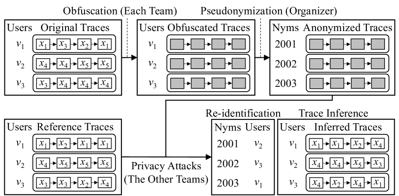
Figure 2. Overview of our contest. Gray squares represent that locations are obfuscated.

First of all, an organizer in our contest performs pseudonymization (which is important but technically trivial) in place of each team to guarantee that pseudonymization is appropriately done. Thus, each team obfuscates traces and sends the traces to the organizer. Then the organizer pseudonymizes the traces, i.e., randomly shuffles the traces and adds pseudonyms.

Each team obfuscates its original traces so that its anonymized traces are secure against trace inference while keeping high utility. Then the other teams attempt both re-identification and trace inference against the anonymized traces. Here, we follow a threat model in the previous work (Gambs et al., 2014; Mulder et al., 2008; Pyrgelis et al., 2017, 2018; Shokri et al., 2011), where the adversary’s background knowledge is separated from the original traces. Specifically, the other teams perform the re-identification and trace inference attacks using reference traces, which are separated from the original traces. Note that they do not know the original traces, i.e., the partial-knowledge attacker model (Ruiz et al., 2018; Murakami and Takahashi, 2021). The reference traces are, for example, traces of the same users on different days. The users may disclose the reference traces via geo-social network services, or the adversary may obtain the reference traces by observing the users in person. The reference traces play a role as background knowledge of the adversary.

For each team, we evaluate the following three scores: utility score, re-identification privacy score, and trace inference privacy score. Every score takes a value between $0$ and $1$ (higher is better). We regard an anonymized trace as valid (resp. invalid) if its utility score is larger than or equal to (resp. below) a pre-determined threshold. For an invalid trace, we set its privacy scores to $0$.

Then we give the best anonymization award to a team that achieves the highest trace inference privacy score. We also give the best re-identification (resp. trace inference) award to a team that contributes the most in lowering re-identification (resp. trace inference) privacy scores for the other teams.

The best anonymization award motivates each team to anonymize traces so that they are secure against trace inference. The other two awards motivate each team to make every effort to attack them in terms of both re-identification and trace inference. Consequently, we can see whether anonymized traces intended to have security against trace inference are also secure against re-identification.

Remark 1.  Note that each team competes for privacy while satisfying the utility requirement in our contest. Each team does not compete for utility while satisfying the privacy requirement, because we would like to investigate the relationship between two privacy risks: re-identification and trace inference.

Remark 2.  It is also possible to design a contest that releases aggregate location time-series (time-dependent population distributions) (Pyrgelis et al., 2018). Our contest follows a general location privacy framework in (Shokri et al., 2011) and releases anonymized traces. This is because the anonymized traces are useful for a very wide range of applications such as POI recommendation (Liu et al., 2017) and geo-data analysis, as shown in Section 5.5.

Remark 3.  As described in Section 2, the attacker can be divided into two types: partial-knowledge attacker (Ruiz et al., 2018; Murakami and Takahashi, 2021) and maximum-knowledge attacker (Domingo-Ferrer et al., 2015). Clearly, the maximum-knowledge attacker is stronger than the partial-knowledge attacker. Our contest focuses on the partial-knowledge attacker model for two reasons. First, the maximum-knowledge attacker model is overly pessimistic; e.g., we need to sacrifice the utility to prevent re-identification in this model (de Montjoye et al., 2013). Second, we cannot evaluate the attribute inference risk in the maximum-knowledge attacker model, as described in Section 2.

Regarding privacy metrics, we can consider the following two types, depending on how to quantify the total risk: average metrics and worst-case metrics. The average metrics consider an average risk over all users, and their examples include the re-identification rate (Gambs et al., 2014; Mulder et al., 2008; Murakami et al., 2021) and the adversary’s expected error (Shokri et al., 2011). In contrast, the worst-case metrics consider a worst-case risk, and their examples include DP (Dwork and Roth, 2014) and its variants (Desfontaines and Pejó, 2020). The worst-case metrics are stronger than the average metrics.

As will be explained later, our contest uses the average metrics – our re-identification and trace inference privacy scores are based on the re-identification rate and the adversary’s expected error, respectively. This is because the worst-case metrics such as DP might result in no meaningful privacy guarantees or poor utility for long traces (Andrés et al., 2013; Pyrgelis et al., 2017), as described in Section 1. Our contest considers DP out of scope in that it does not use DP as a privacy metric. We also note that we do not systematically evaluate actual privacy-utility trade-offs of existing DP algorithms when releasing long traces, which could be an interesting avenue for future work.

3.3. Datasets

Dataset Issue in the Partial-Knowledge Attacker Model.  As described in Section 3.2, our contest assumes the partial-knowledge attacker model, where the adversary does not know the original traces and has reference traces separated from the original ones. In this case, it is challenging to prepare a contest dataset.

Specifically, the challenge in the partial-knowledge attacker model is that public datasets (e.g., (Zheng et al., 2010; Cho et al., 2011; Nightley and Center for Spatial Information Science at the University of Tokyo (2014), CSIS; Yang et al., 2019)) cannot be directly used for a contest. This issue comes from the fact that everyone can access public datasets. In other words, if we use a public dataset for a contest, then every team would know the original traces of the other teams, which leads to the maximum-knowledge attacker model. It is also difficult to directly use a private dataset in a company due to privacy concerns.

One might think that the organizer can use a public dataset by setting a rule that submissions (obfuscated traces) must not include knowledge from the public dataset. However, this is an unrealistic solution because we cannot detect the rule violation. Specifically, we cannot verify whether or not submissions include knowledge from the public dataset, unless we accurately extract information about the public dataset from the submissions, e.g., membership inference (Jayaraman and Evans, 2019; Shokri et al., 2017). The same applies to the case when the submissions are machine learning models, hyperparameters, or architectures – they can be trained from a public dataset to provide better classification accuracy (Bergstra and Bengio, 2012; Elsken et al., 2019), and we cannot detect the rule violation unless we accurately extract the public dataset from them.

One might also think that the organizer can use a public dataset without announcing which public dataset it is. This is also unrealistic for two reasons. First, the number of public datasets is limited. Therefore, each team can easily obtain the public dataset corresponding to reference traces of other teams. In other words, it is very difficult (or impossible) to hide which public dataset is used. Second, we cannot detect the rule violation (i.e., the use of the public dataset corresponding to reference traces), as explained above.

A lot of existing work (Bindschaedler and Shokri, 2016; Chen et al., 2012a, b; Chow and Golle, 2009; He et al., 2015; Kido et al., 2005; Murakami et al., 2021; You et al., 2007) proposes location synthesizers, which take location traces (called training traces) as input and output synthetic traces. However, they cannot be used for our contest. Specifically, most of them (Chen et al., 2012a, b; Chow and Golle, 2009; He et al., 2015; Kido et al., 2005; You et al., 2007) generate synthetic traces based on parameters common to all users and do not provide user-specific features; e.g., someone lives in Manhattan, and another one commutes by train. Note that the user-specific features are necessary for an anonymization contest because otherwise, the adversary cannot re-identify traces. In other words, the adversary needs some user-specific features as background knowledge to re-identify traces.

A handful of existing synthesizers (Bindschaedler and Shokri, 2016; Murakami et al., 2021) preserve the user-specific features. However, both (Bindschaedler and Shokri, 2016) and (Murakami et al., 2021) generate traces so that the $i$-th synthetic trace preserves the user-specific feature of the $i$-th training trace. Thus, if the organizer uses a public dataset as training traces and discloses synthetic traces, each team can obtain the corresponding training traces in the public dataset. Note that even if the organizer shuffles synthetic traces or generates multiple traces per training trace, each team may link each synthetic trace with the corresponding training trace via re-identification to obtain better background knowledge. For example, it is reported in (Murakami et al., 2021) that the synthetic traces in (Bindschaedler and Shokri, 2016) can be easily re-identified (re-identification rate $=80$ to $90\%$) when they preserve statistical information about the training traces. In addition, the synthesizers in (Bindschaedler and Shokri, 2016; Murakami et al., 2021) do not provide strong theoretical privacy guarantees such as DP (Dwork, 2006; Dwork and Roth, 2014) when a private dataset is used as training traces.

Therefore, neither public datasets, private datasets, nor existing location synthesizers can be used for our contest.

Location Synthesizer with Diversity.  To address the dataset issue explained above, we introduce a location synthesizer that takes training traces as input and outputs different synthetic traces for each team. Figure 3 shows its overview. In a nutshell, our location synthesizer randomly generates traces of virtual users who are different from users in the input dataset (called training users), as indicated by different colors in Figure 3. The virtual users for each team are also different from the virtual users for the other teams.

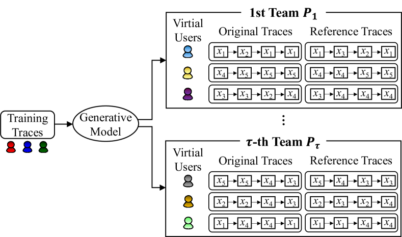
Figure 3. Overview of our location synthesizer.

In our location synthesizer, each virtual user has her own user-specific feature (e.g., live in Manhattan, commute by train) represented as a multi-dimensional vector. We call it a feature vector. We synthesize each user’s trace based on the feature vector. Consequently, each team’s synthetic traces have different features than those of training traces and the other teams’ synthetic traces. We call this diversity of synthetic traces. The diversity prevents the $t$-th team $P_{t}$ from linking the other teams’ reference traces with training traces or $P_{t}$’s original traces to obtain better background knowledge. The organizer does not disclose each team’s original traces or feature vectors to the other teams. Thus, each team does not know the original traces of the other teams, i.e., the partial-knowledge attacker model.

We extend the location synthesizer in (Murakami et al., 2021), which preserves various statistical features of training traces (e.g., distribution of visit-fractions (Do and Gatica-Perez, 2013; Ye et al., 2011), time-dependent population distribution (Zheng et al., 2009), and transition matrix (Liu et al., 2013; Song et al., 2006)), to have diversity explained above. See Appendix A for details of our location synthesizer. In Appendix B, we show through experiments that our synthesizer has diversity and preserves various statistical features. In Appendix C, we also empirically evaluate the privacy of our location synthesizer when a private dataset is used as training traces.

In our contest, we slightly modified our synthesizer in Appendix A to make synthetic traces more realistic in that users tend to be at their home between 8:00 and 9:00 and 17:00 and 18:00 while keeping statistical information (e.g., population distribution, transition matrix). See Appendix D for details. We also published our synthesizer as open-source software (Loc, 2022).

Generation of Traces.  We generate synthetic traces for each team using our location synthesizer. Specifically, we use the SNS-based people flow data (Nightley and Center for Spatial Information Science at the University of Tokyo (2014), CSIS) (Tokyo) as training traces of our location synthesizer. We divide Tokyo equally into $32\times 32$ regions ($1024$ regions in total) and assign region IDs sequentially from lower-left to upper-right. The size of each region is approximately $347$m (height) $\times$ $341$m (width). The left panel of Figure 4 shows the regions in our contest.

Let $m\in\mathbb{N}$ be the number of virtual users for each team. From the training traces, we generate synthetic traces of $m=2000$ virtual users for each team using our location synthesizer. For each virtual user, we generate traces from 8:00 to 18:00 for 40 days with a time interval of 30 minutes. We use traces of the former 20 days as reference traces and the latter 20 days as original traces. Here, we set the reference trace length to 20 days because the existing work assumes such a long reference trace, e.g., two years (Gambs et al., 2014), one month (Mulder et al., 2008), or two to three weeks (Pyrgelis et al., 2017, 2018). Let $l_{o},l_{r}\in\mathbb{N}$ be the length of a training trace and reference trace, respectively. Then $l_{o}=l_{r}=400$. Table 1 summarizes location data in our contest.

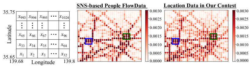
Figure 4. Regions and population distributions at 12:00. Blue and green squares represent Shinjuku and Akihabara, respectively. These areas are crowded in both the SNS-based people flow data and location data in our contest.

Table 1. Location Data in Our Contest

Number of users $m=2000$ Number of regions $1024$ ($=32\times 32$) Trace length $l_{o}=l_{r}=400$ (from $8:00$ to $18:00$ for $20$ days with $30$ minutes interval)

The middle and right panels of Figure 4 show population distributions at 12:00 in the SNS-based people flow data and synthetic traces in our contest, respectively. These panels show that the synthetic traces preserve the time-dependent population distribution.

Let $O^{(t)}$ and $R^{(t)}$ be sets of original traces and reference traces for the $t$-th team $P_{t}$, respectively.

3.4. Details of Our Contest

Below we describe the details of our contest such as scenarios, threat models, contest flow, anonymization, privacy attacks, and utility and privacy scores.

Scenarios and Threat Models.  There are two possible scenarios in our contest. The first scenario is geo-data analysis in a centralized model (Dwork and Roth, 2014), where an LBS provider anonymizes location traces before providing them to a (possibly malicious) data analyst. In this scenario, the data analyst can be an adversary.

The second scenario is LBS with an intermediate server (Bettini et al., 2005; Gedik and Liu, 2008). In this scenario, each user sends her traces to a trusted intermediate server. Then the intermediate server anonymizes the traces of the users and sends them to a (possibly malicious) LBS provider. Finally, each user receives some services (i.e., personalized POI recommendation (Cheng et al., 2013; Feng et al., 2015; Liu et al., 2017)) from the LBS provider through the intermediate server based on her anonymized traces. Consider successive personalized POI recommendation (or next POI recommendation) (Cheng et al., 2013; Feng et al., 2015) as an example. In this service, the LBS provider recommends a list of nearby POIs for each location visited by her. For example, if Alice visits a coffee shop in the morning, a university at noon, and a restaurant in the evening, then the LBS provider recommends POIs nearby the coffee shop, university, and restaurant. In this scenario, the LBS provider can be an (honest-but-curious) adversary.

In both of the scenarios, an adversary does not know the original traces and obtains the anonymized traces. The adversary performs privacy attacks using reference traces of 20 days, which are separated from the original traces. This is consistent with the existing work that assumes such a long reference trace (Gambs et al., 2014; Mulder et al., 2008; Pyrgelis et al., 2017, 2018).

Contest Flow.  Figure 5 shows our contest flow. In our contest, an organizer plays a role as a judge who distributes traces for each team and evaluates privacy and utility scores of each team. Note that the judging process (i.e., sending traces and calculating scores) can be automated. Let $Q$ be a judge. Teams $P_{1},\cdots,P_{\tau}$ and judge $Q$ participate in our contest.

In the anonymization phase, judge $Q$ distributes original traces $O^{(t)}$ to each team $P_{t}$. Team $P_{t}$ obfuscates $O^{(t)}$. Let $O^{*(t)}$ be obfuscated traces of team $P_{t}$. Team $P_{t}$ submits obfuscated traces $O^{*(t)}$ to $Q$. After receiving $O^{*(t)}$, $Q$ pseudonymizes $O^{*(t)}$ by randomly shuffling $m$ traces in $O^{*(t)}$ and then sequentially assigning pseudonyms. Consequently, $Q$ obtains anonymized traces $A^{(t)}$ and an ID table $f^{(t)}$, which is a set of pairs between user IDs and pseudonyms. $Q$ keeps $f^{(t)}$ secret.

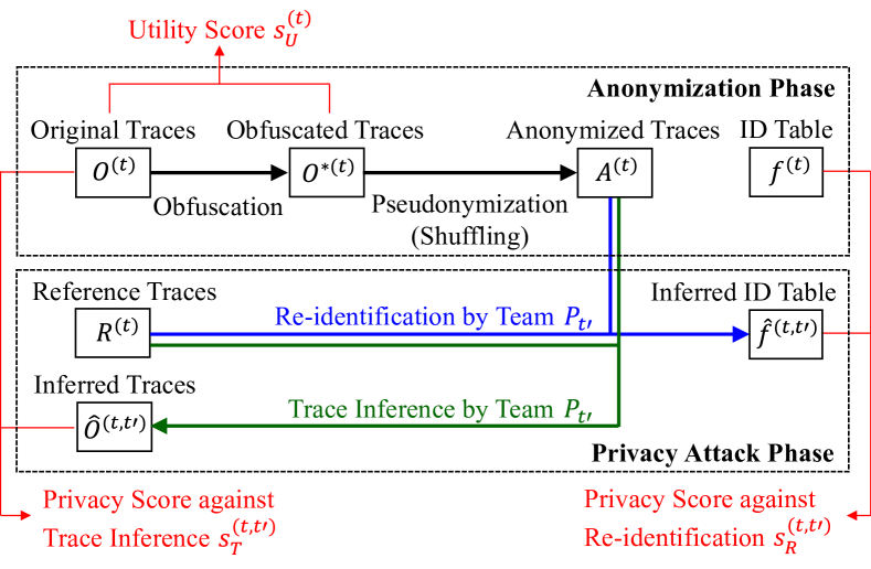
Figure 5. Contest flow for team $P_{t}$ ($t\in[\tau]$). Re-identification and trace inference are performed by another team $P_{t^{\prime}}$ ($t^{\prime}\neq t$). Utility and privacy scores are calculated by judge $Q$.

Judge $Q$ calculates a utility score $s_{U}^{(t)}\in[0,1]$ using original traces $O^{(t)}$ and obfuscated traces $O^{*(t)}$. Then $Q$ compares $s_{U}^{(t)}$ with a threshold $s_{req}\in[0,1]$ that is publicly available. If $s_{U}^{(t)}\geq s_{req}$, then $Q$ regards anonymized traces $A^{(t)}$ as valid (otherwise, invalid). Note that $s_{U}^{(t)}$ is calculated from $O^{(t)}$ and $O^{*(t)}$. Thus, $P_{t}$ can check whether $A^{(t)}$ are valid before submitting $O^{*(t)}$ to $Q$.

In the privacy attack phase, judge $Q$ distributes all reference traces and all valid anonymized traces to all teams. Then each team attempts re-identification and trace inference against the valid anonymized traces of the other teams using their reference traces.

Assume that team $P_{t^{\prime}}$ ($t^{\prime}\neq t$) attacks valid anonymized traces $A^{(t)}$ of team $P_{t}$. As re-identification, team $P_{t^{\prime}}$ infers user IDs corresponding to pseudonyms in $A^{(t)}$ using reference traces $R^{(t)}$. Team $P_{t^{\prime}}$ creates an inferred ID table $\hat{f}^{(t,t^{\prime})}$, which is a set of pairs between inferred user IDs and pseudonyms, and submits it to judge $Q$. As trace inference, team $P_{t^{\prime}}$ infers all locations in original traces $O^{(t)}$ from $A^{(t)}$ using $R^{(t)}$. Team $P_{t^{\prime}}$ creates inferred traces $\hat{O}^{(t,t^{\prime})}$, which include the inferred locations, and submits it to $Q$.

Judge $Q$ calculates a re-identification privacy score $s_{R}^{(t,t^{\prime})}\in[0,1]$ using ID table $f^{(t)}$ and inferred ID table $\hat{f}^{(t,t^{\prime})}$. $Q$ also calculates a trace inference privacy score $s_{T}^{(t,t^{\prime})}\in[0,1]$ using original traces $O^{(t)}$ and inferred traces $\hat{O}^{(t,t^{\prime})}$.

Note that anonymized traces $A^{(t)}$ get $\tau-1$ attacks from the other teams. They also get attacks from some sample algorithms for re-identification and trace inference, which are described in Section 4. Judge $Q$ calculates privacy scores against all of these attacks and finds the minimum privacy score. Let $s_{R,min}^{(t)}$ (resp. $s_{T,min}^{(t)}$) $\in[0,1]$ be the minimum re-identification (resp. trace inference) privacy score of team $P_{t}$. $s_{R,min}^{(t)}$ and $s_{T,min}^{(t)}$ are final privacy scores of team $P_{t}$; i.e., we adopt a privacy score by the strongest attack.

Pseudonymized Traces.  In the privacy attack phase, judge $Q$ also distributes pseudonymized traces prepared by $Q$ and makes each team attack these traces. The purpose of this is to compare the privacy of each team’s anonymized traces with that of the pseudonymized traces; i.e., they play a role as a benchmark.

The pseudonymized traces are generated as follows. Judge $Q$ generates reference traces $R^{(\tau+1)}$ and original traces $O^{(\tau+1)}$ for team $P^{(\tau+1)}$ (who does not participate in the contest). Then $Q$ makes anonymized traces $A^{(\tau+1)}$ by only pseudonymization. Finally, $Q$ distributes $A^{(\tau+1)}$ and $R^{(\tau+1)}$, and each team $P_{t}$ attempts privacy attacks against $A^{(\tau+1)}$ using $R^{(\tau+1)}$.

Sample Traces.  Judge $Q$ also generates reference and original traces of two teams $P^{(\tau+2)}$ and $P^{(\tau+3)}$ (who do not participate in the contest) as sample traces. $Q$ distributes the sample traces to all teams in the anonymization phase. The purpose of distributing sample traces is to allow each team to tune parameters in her anonymization and privacy attack algorithms.

Awards.  As described in Section 3.2, awards are important to make both defense and attack complete together. We give the best anonymization award to a team $P_{t}$ who achieves the highest trace inference privacy score $s_{T,min}^{(t)}$ among all teams. We also give the best re-identification (resp. trace inference) award to a team $P_{t^{\prime}}$ whose $\sum_{t=1}^{\tau+1}s_{R}^{(t,t^{\prime})}$ (resp. $\sum_{t=1}^{\tau+1}s_{T}^{(t,t^{\prime})}$) is the lowest among all teams.

Fairness.  It should be noted that the diversity of location traces may raise a fairness issue. For example, even if all teams apply the same anonymization and attack algorithms, privacy scores can be different among the teams.

In Appendix E, we evaluate the fairness of our contest. Specifically, we evaluate the variance of privacy scores against the same attack algorithm and show that it is small. For example, the standard deviation of re-identification privacy scores is about $0.01$ or less, which is much smaller than the difference between the best privacy score ($=0.79$) and the second-best privacy score ($=0.67$). See Appendix E for more details.

Anonymization.  In the anonymization phase, team $P_{t}$ obfuscates its original traces $O^{(t)}$. In our contest, we allow four types of processing for each location:

1. No Obfuscation: Output the original location as is; e.g., $x_{1}\rightarrow x_{1}$.

2. Perturbation (Adding Noise): Replace the original location with another location; e.g., $x_{1}\rightarrow x_{2}$.

3. Generalization: Replace the original location with a set of multiple locations; e.g., $x_{1}\rightarrow\{x_{1},x_{3}\}$, $x_{1}\rightarrow\{x_{2},x_{3},x_{5}\}$. Note that the original location may not be included in the set.

4. Deletion: Replace the original location with an empty set $\emptyset$ representing deletion; e.g., $x_{1}\rightarrow\emptyset$.

Let $\mathcal{Y}$ be a finite set of outputs after applying one of the four types of processing to a location. Then $\mathcal{Y}$ is represented as a power set of $\mathcal{X}$; i.e., $\mathcal{Y}=2^{\mathcal{X}}$. In other words, we accept all possible operations on each location.

Then judge $Q$ pseudonymizes obfuscated traces $O^{*(t)}$. Specifically, judge $Q$ randomly permutes $1,\cdots,m$ and sequentially assign pseudonyms $m+1,\cdots,2m$.

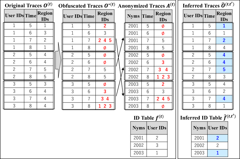
Figure 6. Example of anonymization and privacy attacks. Obfuscated locations are marked with bold red font. “2 4 5” represents generalized locations $\{x_{2},x_{4},x_{5}\}$. “$\emptyset$” represents deletion. Correct user/region IDs are marked with bold blue font on a light blue background.

The left panel of Figure 6 shows an example of anonymization, where user IDs and region IDs are subscripts of users and regions, respectively. In this example, pseudonyms $2001$, $2002$, and $2003$ correspond to user IDs $2$, $3$, and $1$, respectively; i.e., $f^{(t)}=\{(2001,2),(2002,3),(2003,1)\}$.

Privacy Attack.  In the privacy attack phase, team $P_{t^{\prime}}$ ($t^{\prime}\neq t$) attempts privacy attacks against (valid) anonymized traces $A^{(t)}$ of team $P_{t}$ using reference traces $R^{(t)}$. Specifically, team $P_{t^{\prime}}$ creates an inferred ID table $\hat{f}^{(t,t^{\prime})}$ and inferred traces $\hat{O}^{(t,t^{\prime})}$ for re-identification and trace inference, respectively. Here we allow $P_{t^{\prime}}$ to identify multiple pseudonyms in $A^{(t)}$ as the same user ID.

The right panel of Figure 6 shows an example of privacy attacks. In this example, $\hat{f}^{(t,t^{\prime})}=\{(2001,2),(2002,2),\allowbreak(2003,1)\}$.

Utility Score.  Anonymized traces $A^{(t)}$ are useful for geo-data analysis, e.g., mining popular POIs (Zheng et al., 2009), auto-tagging POI categories (Do and Gatica-Perez, 2013; Ye et al., 2011), and modeling human mobility patterns (Liu et al., 2013; Song et al., 2006). They are also useful for LBS in the intermediate server model (as described in Section 3.4 “Scenarios and Threat Models”). For example, in the successive personalized POI recommendation (Cheng et al., 2013; Feng et al., 2015), it is important to preserve rough information about each location in the original traces. Thus, a location synthesizer that preserves only statistical information about the original traces is not useful as an anonymization method in the latter scenario. To accommodate a variety of purposes, we adopt a versatile utility score $s_{U}^{(t)}\in[0,1]$.

Specifically, for both geo-data analysis and LBS, it would be natural to consider that the utility degrades as the distance between an original location and a noisy location becomes larger. The utility would be completely lost when the distance exceeds a certain level or when the original location is deleted.

Taking this into account, we define the utility score $s_{U}^{(t)}$. Our utility score is similar to the service quality loss (SQL) (Andrés et al., 2013; Bordenabe et al., 2014; Shokri et al., 2012) for perturbation in that the utility is measured by the expected Euclidean distance between original locations and obfuscated locations. Our utility score differs from the SQL in two ways: (i) we deal with perturbation, generalization, and deletion; (ii) we assume the utility is completely lost when the distance exceeds a certain level or the original location is deleted.

Formally, let $d:\mathcal{X}\times\mathcal{X}\rightarrow\mathbb{R}_{\geq 0}$ be a distance function that takes two locations $x_{i},x_{j}\in\mathcal{X}$ as input and outputs their Euclidean distance $d(x_{i},x_{j})\in\mathbb{R}_{\geq 0}$. Since the location data are regions in our contest, we define $d(x_{i},x_{j})$ as the Euclidean distance between center points of region $x_{i}$ and $x_{j}$. For example, $d(x_{1},x_{2})=341$m and $d(x_{1},x_{34})=\sqrt{347^{2}+341^{2}}=487$m in our contest, as the size of each region is $347$m (height) $\times$ $341$m (width).

We calculate the Euclidean distance between each location in $O^{(t)}$ and the corresponding location(s) in $O^{*(t)}$. For $i\in[m]$ and $j\in[l_{o}]$, let $\alpha_{i,j}^{(t)}\in\mathbb{R}_{\geq 0}$ be the Euclidean distance between the $j$-th locations in the original and obfuscated traces for user $v_{i}^{(t)}$. $\alpha_{i,j}^{(t)}$ takes the average Euclidean distance for generalization, and $\infty$ for deletion. For example, $\alpha_{1,1}^{(t)}=d(x_{1},x_{2})$, $\alpha_{1,2}^{(t)}=d(x_{3},x_{3})=0$, $\alpha_{1,3}^{(t)}=\frac{d(x_{2},x_{2})+d(x_{2},x_{4})+d(x_{2},x_{5})}{3}$, and $\alpha_{1,4}^{(t)}=\infty$ in Figure 6.

Finally, we use a piecewise linear function $g_{U}$ shown in the left of Figure 7 to transform each $\alpha_{i,j}^{(t)}$ into a score value from $0$ to $1$ (higher is better). Then we calculate the utility score $s_{U}^{(t)}$ by taking the average of $ml_{o}$ scores.

Figure 7. Piecewise linear functions $g_{U}$ and $g_{T}$.

Specifically, let $g_{U}:\mathbb{R}_{\geq 0}\rightarrow[0,1]$ be a function that takes $\alpha\in\mathbb{R}_{\geq 0}$ as input and outputs the following score:

$$g_{U}(\alpha)=\begin{cases}1-\frac{\alpha}{\lambda_{U}}&\text{(if $\alpha<\lambda_{U}$)}\\ 0&\text{(if $\alpha\geq\lambda_{U}$)},\end{cases}$$

where $\lambda_{U}\in\mathbb{R}_{\geq 0}$ is a threshold. Using this function, we calculate the utility score $s_{U}^{(t)}$ as follows:

$$\textstyle{s_{U}^{(t)}=\frac{1}{ml_{o}}\sum_{i=1}^{m}\sum_{j=1}^{l_{o}}g_{U}(\alpha_{i,j}^{(t)}).}$$

For example, if we do not obfuscate any location, then $s_{U}^{(t)}=1$. If we delete all locations or the Euclidean distance exceeds $\lambda_{U}$ for all locations, then $s_{U}^{(t)}=0$.

In our contest, we set the threshold $\lambda_{U}$ to $\lambda_{U}=2$km and the threshold $s_{req}$ of the utility score (for determining whether or not anonymized traces are valid) to $s_{req}=0.7$. In Section 5.5, we also show that valid anonymized traces have high utility for a variety of purposes such as POI recommendation and geo-data analysis.

Re-identification Privacy Score.  A re-identification privacy score $s_{R}^{(t,t^{\prime})}\in[0,1]$ is calculated by comparing ID table $f^{(t)}$ with inferred ID table $\hat{f}^{(t,t^{\prime})}$.

In our contest, we calculate $s_{R}^{(t,t^{\prime})}$ based on the re-identification rate (Gambs et al., 2014; Mulder et al., 2008; Murakami et al., 2021), a proportion of correctly identified pseudonyms. Specifically, we calculate $s_{R}^{(t,t^{\prime})}$ by subtracting the re-identification rate from 1 (higher is better). For example, $s_{R}^{(t,t^{\prime})}=1-\frac{2}{3}=\frac{1}{3}$ in Figure 6.

Trace Inference Privacy Score.  A trace inference privacy score $s_{T}^{(t,t^{\prime})}\in[0,1]$ is calculated by comparing original traces $O^{(t)}$ with inferred traces $\hat{O}^{(t,t^{\prime})}$.

Since Shokri et al. (Shokri et al., 2011) showed that incorrectness determines the privacy of users, the adversary’s expected error has been widely used as a location privacy metric. The expected error is an average distance (e.g., the Euclidean distance (Shokri et al., 2012)) between original locations and inferred locations.

Formally, for $i\in[m]$ and $j\in[l_{o}]$, let $\beta_{i,j}^{(t,t^{\prime})}\in\mathbb{R}_{\geq 0}$ be the Euclidean distance between the $j$-th locations in the original and inferred traces for user $v_{i}^{(t)}$. For example, $\beta_{1,1}^{(t,t^{\prime})}=d(x_{1},x_{1})$, $\beta_{1,2}^{(t,t^{\prime})}=d(x_{3},x_{1})$, $\beta_{1,3}^{(t,t^{\prime})}=d(x_{2},x_{2})$, and $\beta_{1,4}^{(t,t^{\prime})}=d(x_{1},x_{4})$ in Figure 6. Then, the expected error with the Euclidean metric is given by:

(1) $${\color[rgb]{0,0,0}\textstyle{\frac{1}{ml_{o}}\sum_{i=1}^{m}\sum_{j=1}^{l_{o}}\beta_{i,j}^{(t,t^{\prime})}.}}$$

In our contest, we use the expected error with two modifications. First, we want all utility and privacy scores to be between 0 and 1 (higher is better) so that they are easy to understand for all teams. Thus, we transform the Euclidean distance into a score value from $0$ to $1$. Specifically, we assume that the adversary completely fails to infer the original location when the distance exceeds a certain level. In other words, we use a piecewise linear function $g_{T}$ in the right of Figure 7 to transform each $\beta_{i,j}^{(t,t^{\prime})}$ into a score value from $0$ to $1$ (higher is better). Formally, let $g_{T}:\mathbb{R}_{\geq 0}\rightarrow[0,1]$ be a function that takes $\beta\in\mathbb{R}_{\geq 0}$ as input and outputs the following score:

$$g_{T}(\beta)=\begin{cases}\frac{\beta}{\lambda_{T}}&\text{(if $\beta<\lambda_{T}$)}\\ 1&\text{(if $\beta\geq\lambda_{T}$)},\end{cases}$$

where $\lambda_{T}\in\mathbb{R}_{\geq 0}$ is a threshold. In our contest, we set $\lambda_{T}=2$km. By using $g_{T}$, we obtain $ml_{o}$ scores.

Second, we consider regions that include hospitals (referred to as hospital regions) to be especially sensitive. There are $37$ hospital regions in the SNS-based people flow data (Nightley and Center for Spatial Information Science at the University of Tokyo (2014), CSIS). Since sensitive locations need to be carefully handled, we calculate the privacy score $s_{T}^{(t,t^{\prime})}$ by taking a weighted average of $ml_{o}$ scores, where we set a weight value to $10$ for hospital regions and $1$ for the others.

Thus, we calculate the privacy score $s_{T}^{(t,t^{\prime})}$ as:

(2) $$\textstyle{s_{T}^{(t,t^{\prime})}=\frac{\sum_{i=1}^{m}\sum_{j=1}^{l_{o}}w_{i,j}g_{T}(\beta_{i,j}^{(t,t^{\prime})})}{\sum_{i=1}^{m}\sum_{j=1}^{l_{o}}w_{i,j}},}$$

where $w_{i,j}\in\{1,10\}$ is a weight variable that takes $10$ if the $j$-th location in the original trace of user $v_{i}^{(t)}$ is a hospital region, and $1$ otherwise. If the inferred traces are perfectly correct ($O^{(t)}=\hat{O}^{(t,t^{\prime})}$), then $s_{T}^{(t,t^{\prime})}=0$.

We set a hospital weight to $10$ because a too large value results in a low correlation between our privacy score and the expected error, as shown in Section 5.4. In other words, if we choose a too large hospital weight, the best anonymization algorithm loses its versatility – it may not be useful when the expected error is used as a privacy metric. Our privacy score with hospital weight $=10$ carefully handles sensitive regions (as hospital weight $\gg 1$) and is yet highly correlated with the expected error.

Remark.  Because our utility/privacy scores are based on the existing metrics (i.e., SQL (Andrés et al., 2013; Bordenabe et al., 2014; Shokri et al., 2012), re-identification rate (Gambs et al., 2014; Mulder et al., 2008; Murakami et al., 2021), and the expected error (Shokri et al., 2011)), they are also useful for evaluating anonymization techniques in research papers. One difference between our contest and academic research is that both defense and attack compete together (i.e., each team attacks other teams) in our contest. Such evaluation might be difficult for academic research.

4. Preliminary Experiments

Prior to our contest, we conducted preliminary experiments. The main purpose of the preliminary experiments is to show that the cheating anonymization (Kikuchi et al., 2016a), which is perfectly secure against re-identification as described in Section 1, is not secure against trace inference. This result serves as strong evidence that trace inference should be added as an additional risk in our contest. Another purpose is to make all teams understand how to perform obfuscation, re-identification, and trace inference. To this end, we implemented some sample algorithms and released all the sample algorithms and the experimental results to all teams before the contest. Section 4.1 explains our experimental set-up. Section 4.2 reports our experimental results.

4.1. Experimental Set-up

Dataset.  We used the SNS-based people flow data (Nightley and Center for Spatial Information Science at the University of Tokyo (2014), CSIS) (Osaka). We divided Osaka into $32\times 32$ regions ($1024$ regions in total), and extracted training traces from 8:00 to 18:00 for $4071$ users. We trained our location synthesizer using the training traces.

Then we generated reference traces $R^{(0)}$ and original traces $O^{(0)}$ for $m=2000$ virtual users in one team (whose team number is $t=0$) using our synthesizer. Each trace includes locations from 8:00 to 18:00 for $20$ days with time interval of 30 minutes ($l_{o}=l_{r}=400)$.

Sample Algorithms.  We implemented some sample algorithms for obfuscation, re-identification attacks, and trace inference attacks. We anonymized the original traces $O^{(0)}$ by using each sample obfuscation algorithm. Then we performed privacy attacks by using each sample re-identification or trace inference algorithm.

For obfuscation, we implemented the following algorithms:

• No Obfuscation: Output the original location as is. In other words, we perform only pseudonymization.

• MRLH($\mu_{x},\mu_{y},\lambda$): Merging regions and location hiding in (Shokri et al., 2011). It generalizes each region in the original trace by dropping lower $\mu_{x}$ (resp. $\mu_{y}$) bits of the $x$ (resp. $y$) coordinate expressed as a binary sequence and deletes the region with probability $\lambda$. For example, the $x$ (resp. $y$) coordinate of $x_{2}$ is $00001$ (resp. $00000$) in Figure 4. Thus, given input $x_{2}$, MRLH($1,1,0.8$) outputs $\{x_{1},x_{2},x_{33},x_{34}\}$ with probability $0.2$ and deletes $x_{2}$ with probability $0.8$.

• RR($\varepsilon$): The $\kappa$-ary randomized response in (Kairouz et al., 2016), where $\kappa$ is the size of input domain ($\kappa=1024$ in our experiments). It outputs the original region with probability $\frac{e^{\varepsilon}}{\kappa-1+e^{\varepsilon}}$, and outputs another region at random with the remaining probability. It provides $\varepsilon$-DP for each region.

• PL($l,r$): The planar Laplace mechanism (Andrés et al., 2013). It perturbs each region in the original trace according to the planar Laplacian distribution so that it provides $l$-DP within $r$ km. This privacy property is known as $\varepsilon$-geo-indistinguishability (Andrés et al., 2013), where $\varepsilon=l/r$.

• Cheat($p$): The cheating anonymization (Kikuchi et al., 2016a). It selects the first $p$ ($0\leq p\leq 1$) of all users as a subset of users, and randomly shuffles the whole traces within the subset (as in Figure 1). Note that this is excessive location obfuscation rather than pseudonymization.

For privacy attacks, we developed two sample algorithms for re-identification (VisitProb-R, HomeProb-R) and two algorithms for trace inference (VisitProb-T, HomeProb-T). All of them are based on a visit probability vector, which comprises the visit probability for each region. We calculate the visit probability vector for each virtual user based on reference traces. Then we perform re-identification or trace inference for each anonymized trace using the visit probability vectors. We published all the sample algorithms as open-source software (PWS, 2019).

Below, we explain each attack algorithm. We also show examples of visit probability vectors, VisitProb-R, and VisitProb-T in Appendix F.

VisitProb-R.  VisitProb-R first trains a visit-probability vector for each user from reference traces. For an element with zero probability, it assigns a very small positive value $\delta$ ($=10^{-8}$) to guarantee that the likelihood never becomes zero.

Then VisitProb-R re-identifies each trace as follows. It computes the likelihood (the product of the likelihood for each region) for each user. For generalized regions, it averages the likelihood over generalized regions. For deletion, it does not update the likelihood. After computing the likelihood for each user, it outputs a user ID with the highest likelihood as an identification result.

HomeProb-R.  HomeProb-R re-identifies traces based on the fact that a user tends to be at her home region between 8:00 and 9:00 (see Appendix D for details). Specifically, it modifies VisitProb-R to use only regions between 8:00 and 9:00.

VisitProb-T.  VisitProb-T first re-identifies traces using VisitProb-R. Here, it does not choose an already re-identified user to avoid duplication of user IDs. Then it de-obfuscates the original regions for each re-identified trace. For perturbation, it outputs the noisy location as is. For generalization, it randomly chooses a region from generalized regions. For deletion, it randomly chooses a region from all regions.

HomeProb-T.  HomeProb-T modifies VisitProb-T to use HomeProb-R for re-identification.

4.2. Experimental Results

Results.  For each sample obfuscation algorithm, we calculated the minimum re-identification (resp. trace inference) privacy score $s_{R,min}^{(0)}$ (resp. $s_{T,min}^{(0)}$) over the sample attack algorithms. Figure 8 shows the results.

Overall, there is a positive correlation between the re-identification privacy score $s_{R,min}^{(0)}$ and the trace inference privacy score $s_{T,min}^{(0)}$. However, there is a clear exception – cheating anonymization. In cheating anonymization, $s_{R,min}^{(0)}$ increases with increase in the parameter $p$. When $p=1$ (i.e., when we shuffle all users), $s_{R,min}^{(0)}$ is almost $1$. In other words, the re-identification rate is almost $0$ for Cheat($1$). This is because the adversary cannot find which permutation is correct, as described in Section 1. Thus, the adversary cannot re-identify traces with higher accuracy than a random guess ($=1/2000$). However, $s_{T,min}^{(0)}$ does not increase with increase in $p$, and $s_{T,min}^{(0)}$ of Cheat($1$) is almost the same as that of No Obfuscation. This means that the adversary can recover the original traces from anonymized traces without accurately re-identifying them.

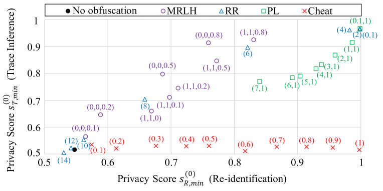
Figure 8. Privacy scores of the sample algorithms (higher is better). The numbers in parentheses represent the parameters in the sample algorithms.

We can explain why this occurs as follows. Suppose that the adversary has reference traces highly correlated with the original traces in the example of Figure 1. First, this adversary would re-identify $10001$ as $v_{2}$, which is incorrect. Then, the adversary may recover the trace of $v_{2}$ as $x_{1}\rightarrow x_{1}\rightarrow x_{1}\rightarrow x_{2}$ because they are included in the anonymized trace of $10001$. This is perfectly correct.

This example explains the intuition that the cheating anonymization is insecure – the adversary can easily recover the original traces from the anonymized traces, even if she cannot accurately re-identify them. Figure 8 clearly shows that the re-identification alone is insufficient as a privacy risk for the cheating anonymization.

Take Aways.  In summary, we should avoid using re-identification alone as a privacy metric when organizing a contest. Otherwise, there is no guarantee that a winning team’s algorithm, which achieves the highest re-identification privacy score, protects user privacy. As described in Section 1, $k$-anonymity is also vulnerable to attribute (location) inference (Machanavajjhala et al., 2006). However, our experimental results provide stronger evidence in that there is an algorithm that is perfectly secure against re-identification and is not secure against trace inference. To make the contest meaningful, we should add trace inference as a risk.

5. Contest Results and Analysis

We released all the sample algorithms and the results of our preliminary experiments to all teams before the contest. Then we held our contest to answer the second question RQ2 in Section 3.1. Section 5.1 reports our contest results. Sections 5.2 and  5.3 explain the best anonymization and privacy attack algorithms that won first place in our contest. Section 5.4 analyzes the relationship between the expected error in (Shokri et al., 2011) and our privacy scores with various weight values. Finally, Section 5.5 shows that the anonymized traces in our contest are useful for various applications.

5.1. Contest Results

Number of Teams.  A total of $21$ teams participated in our contest ($\tau=21$). In the anonymization phase, $18$ teams submitted their obfuscated traces so that the anonymized traces were secure against trace inference. We set the threshold $s_{req}$ of the utility score to $s_{req}=0.7$, as described in Section 3.4. The anonymized traces of $17$ (out of $18$) teams were valid.

In the privacy attack phase, each team attempted re-identification and trace inference against the valid anonymized traces of the other teams and pseudonymized traces prepared by the organizer. Then we evaluated the minimum privacy scores $s_{R,min}^{(t)}$ and $s_{T,min}^{(t)}$ for the anonymized traces of the $17$ teams and the pseudonymized traces.

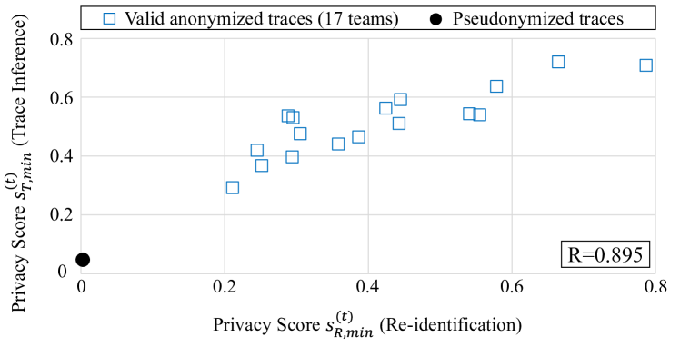
Figure 9. Privacy scores of the valid anonymized traces of the $17$ teams and the pseudonymized traces (higher is better). R is the correlation coefficient between $s_{R,min}^{(t)}$ and $s_{T,min}^{(t)}$.

Results.  Figure 9 shows the results. It shows that there is a strong correlation between the re-identification privacy score $s_{R,min}^{(t)}$ and the trace inference privacy score $s_{T,min}^{(t)}$ (the correlation coefficient is $0.895$). We will discuss the reason for this at the end of Section 5.1.

Figure 9 also shows that the privacy of the pseudonymized traces is completely violated in terms of both re-identification and trace inference. This means that attacks by the teams are much stronger than the sample attacks.

After the contest, all teams presented their algorithms in person. Thus, they learned which algorithm won and why. They also learned that pseudonymization is insufficient by violating pseudonymized traces by themselves. All of them play an educational role.

We also published the submitted files by all the teams (PWS, 2019).

Answer to RQ2 in Section 3.1.  Figure 9 shows that there is a strong correlation between two privacy scores $s_{R,min}^{(t)}$ and $s_{T,min}^{(t)}$.

The reason for this can be explained as follows. In our contest, we gave the best anonymization award to a team that achieved the highest privacy score $s_{T,min}^{(t)}$ against trace inference. Thus, no team used the cheating anonymization that was not effective for trace inference. Consequently, each team had to re-identify traces and then de-obfuscate traces to recover the original traces. In other words, it was difficult to accurately recover the original traces without accurately identifying them. Moreover, all the traces were appropriately pseudonymized (randomly shuffled) by the organizer in our contest. Thus, re-identification was also difficult for traces that were well obfuscated. In this case, the accuracy of re-identification is closely related to the accuracy of trace inference. The team that won the best anonymization award also obfuscated traces so that re-identification was difficult (see Section 5.2 for details).

In summary, under the presence of appropriate pseudonymization, the answer to RQ2 in Section 3.1 was yes in our contest.

5.2. Best Anonymization Algorithm

Below, we briefly explain the best anonymization algorithm that achieved the highest trace inference privacy score $s_{T,min}^{(t)}$. The source code is also published in (PWS, 2019).

The best anonymization team is from a company. The age range is 20s to 30s. The team members have participated in past PWS Cups. They are also a certified business operator of anonymization.

Algorithm.  In a nutshell, the best anonymization algorithm obfuscates traces using $k$-means clustering so that re-identification is difficult within each cluster.

Specifically, the best algorithm consists of three steps: (i) clustering users based on visit count vectors, (ii) adding noise to regions so that visit count vectors are as similar as possible within the same cluster, and (iii) replacing each hospital region with another nearby hospital region. The first and second steps aim at preventing re-identification based on visit probability vectors. In addition, the amount of noise in step (ii) is small because the visit count vectors are similar within the cluster from the beginning. The third step aims at preventing the inference of sensitive hospital regions. The amount of noise in step (iii) is also small because the selected hospital region is close to the original hospital region.

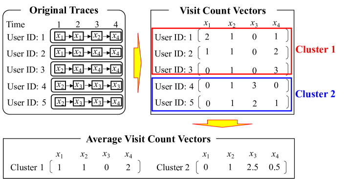
Figure 10. Clusters of visit count vectors.

Specifically, in step (i), it clusters users based on visit count vectors using the $k$-means clustering algorithm, where the number $k$ of clusters is $k=100$. In step (ii), it calculates the average visit count vector within each cluster and adds noise to regions of each trace to move its visit count vector close to the average visit count vector. Steps (ii) and (iii) are performed under the constraint of the utility requirement (utility score $\geq 0.7$). Figure 10 shows a simple example of the clusters ($k=2$) and the average visit count vectors.

Difference from Existing Algorithms.  The best algorithm is based on $k$-means clustering and is somewhat similar to $k$-anonymity based trace obfuscation (Bettini et al., 2009; Chow and Mokbel, 2011; Gedik and Liu, 2008). However, it differs from (Bettini et al., 2009; Chow and Mokbel, 2011; Gedik and Liu, 2008) in that the best algorithm does not provide $k$-anonymity that requires too much noise for long traces. It is well known that both $k$-anonymity and DP could destroy utility for long traces (Andrés et al., 2013; Bettini et al., 2009; Pyrgelis et al., 2017). The best algorithm avoids this issue by obfuscating traces within each cluster so that they are similar rather than identical. The fact that this algorithm won first place suggests that we need to look beyond popular notions such as $k$-anonymity and DP to achieve high utility for long traces.

5.3. Best Attack Algorithms

We also explain attack algorithms for re-identification and trace inference developed by a team that won first place in re-identification (i.e., the best re-identification award) and third place in trace inference. The source code is also published in (PWS, 2019). Although a team that won first place in trace inference is different, we omit its algorithm because the sum of privacy scores against the other teams is similar between the first to fourth teams.

The best attack team is from a company. The age range is 40s. The team members have also participated in past PWS Cups.

Re-identification Algorithm.  The best attack algorithm introduces a fuzzy counting technique as a basic strategy. The fuzzy counting technique counts each region in the reference trace and its surrounding regions ($8$ regions) to construct an attack model.

Specifically, when generating a visit count vector for each user from her reference trace, this technique counts each region in the reference trace (referred to as a target region) and its surrounding regions fuzzily. The fuzzy count for each region is determined by an exponential decay function $h(d)=\eta_{o}e^{-\lambda_{0}d}$, where $\eta_{0}$ and $\lambda_{0}$ are constants and $d$ is the Euclidean distance from the target region. The Euclidean distance is normalized so that the distance between two neighbor regions is $1$. Figure 11 shows an example of the fuzzy counting when $\eta_{0}=0.2$ and $\lambda_{0}=0.5$.

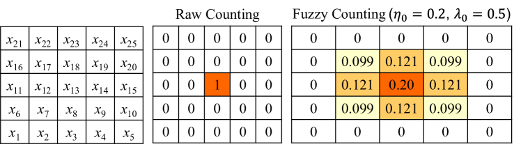
Figure 11. Fuzzy counting. In this example, the target region is $x_{13}$. The raw counting technique simply counts the target region. The fuzzy counting technique increases counts for surrounding regions, e.g., count for $x_{8}$ by $0.121$.

From each visit count vector, it generates a term frequency–inverse document frequency (TF-IDF) style feature vector to weigh unpopular regions more than popular regions. Specifically, let $\gamma_{i,j}\in\mathbb{R}_{\geq 0}$ be a count of region $x_{i}$ in user $u_{j}$’s trace, and $\xi_{i}\in\mathbb{Z}_{\geq 0}$ be the number of users whose trace includes region $x_{i}$ ($\xi_{i}\leq m=2000$). Then it calculates the $i$-th element of the 1024-dim feature vector of user $u_{j}$ by TF $\cdot$ IDF, where (TF, IDF) $=(\gamma_{i,j},\log\frac{m}{\xi_{i}})$, $(\gamma_{i,j},1)$, $(\log(1+\frac{m}{\xi_{i}}),\log\frac{m}{\xi_{i}})$, or $(\log(1+\frac{m}{\xi_{i}}),1)$. Based on the feature vectors, it finds a user ID for each pseudonym via the 1-nearest neighbor search. Optimal values of $\eta_{0}$, $\lambda_{0}$, and (TF, IDF) were determined using sample traces described in Section 3.4. The optimal values were as follows: $\eta_{0}=0.33$, $\lambda_{0}=1$, and (TF, IDF) $=(\log(1+\frac{m}{\xi_{i}}),1)$.

Trace Inference Algorithm.  The trace inference algorithm of this team first re-identifies traces using the re-identification algorithm explained above. Then it de-obfuscates the original regions for each re-identified trace in a similar way to VisitProb-T with an additional technique – replacing frequent regions. The basic idea of this technique is that if a user frequently visits a region in reference traces, then she also frequently visits the region in original traces.

Specifically, from reference traces, this technique calculates a region with the largest visit-count for each user and each time from 8:00 to 18:00. Because the reference trace length is $20$ days, there are $20$ visit-counts in total for each user and each time. If the visit-count exceeds a threshold (determined using sample traces), it regards the region as frequent. Finally, it replaces a region with the frequent region (if any) for each user and each time in the inferred traces.

Difference from Existing Algorithms.  The best attack algorithm uses a fuzzy counting technique as a basic strategy. Existing work (Gambs et al., 2014; Mulder et al., 2008; Shokri et al., 2011) and our sample algorithms in Section 4.1 only count each region in the reference trace to construct an attack model. Thus, the fuzzy counting technique is more robust to small changes in the locations. In fact, the best algorithm provides much better attack accuracy than our sample algorithms.

Fuzzy counting is also simple and much more efficient than complicated attacks such as (Murakami, 2017; Murakami et al., 2017). Specifically, let $\eta\in\mathbb{N}$ be the total number of regions. Then, the time complexity of fuzzy counting is $O(m(l_{r}+\eta))$, whereas that of (Murakami, 2017; Murakami et al., 2017) is $O(ml_{r}\eta^{2})$.

5.4. Relationship with the Expected Error

In our contest, we used a trace inference privacy score $s_{T}^{(t,t^{\prime})}$ with hospital weight $=10$. Below, we analyze the relationship between the expected error (Shokri et al., 2011) and our privacy scores $s_{T}^{(t,t^{\prime})}$ with various hospital weights.

The left panel of Figure 12 shows the relationship between our privacy score with hospital weight $=10$ and the expected error. Here, we used the valid anonymized traces of the $17$ teams and the pseudonymized traces in our contest. We observe that our privacy score with hospital weight $=10$ is highly correlated with the expected error – the correlation coefficient is R $=0.937$.

The right panel of Figure 12 shows the relationship between the correlation coefficient R and the hospital weight. We observe that as the hospital weight increases from $10$, R rapidly decreases; e.g., R $=0.846$ and $0.811$ when hospital weight $=100$ and $1000$, respectively. This means that if we choose such large weights, the best anonymization algorithm loses its versatility – it may not be useful when the expected error is used as a privacy metric. In contrast, the best anonymization algorithm in our contest carefully handles sensitive regions (as hospital weight $\gg 1$) and also provides the largest expected error, as shown in the left panel of Figure 12.

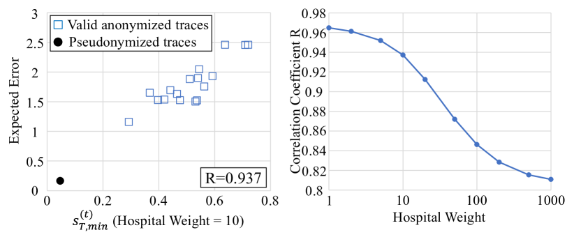
Figure 12. Relationship between our trace inference privacy scores with various hospital weights and the expected error (Shokri et al., 2011). R is the correlation coefficient.

5.5. Utility in Our Contest

We finally analyzed the utility of the valid anonymized traces of the $17$ teams for various applications as follows.

POI Recommendation.  As described in Section 3.4, anonymized traces are useful for POI recommendation (Cheng et al., 2013; Feng et al., 2015; Liu et al., 2017) in the intermediate model. In our analysis, we considered the following successive personalized POI recommendation. Suppose that a user is interested in POIs within a radius of $r_{1}$ km from each location in her original trace (referred to as nearby POIs). To recommend the nearby POIs, the LBS provider sends all POIs within a radius of $r_{2}$ km from each location in the anonymized trace to the user through the intermediate server. Then the client application makes a recommendation of POIs based on the received POIs.

Note that the client application knows the original locations. Therefore, it can filter the received POIs, i.e., exclude POIs outside of the radius of $r_{1}$ from the original locations. Thus, $r_{2}$ can be set to be larger than $r_{1}$ to increase the accuracy at the expense of higher communication cost (Andrés et al., 2013).

We extracted POIs in the “food” category from the SNS-based people flow data (Nightley and Center for Spatial Information Science at the University of Tokyo (2014), CSIS) ($4692$ POIs in total). We set $r_{1}=1$ km and $r_{2}=2$ km. Then we evaluated the proportion of nearby POIs included in the received POIs to the total number of nearby POIs and averaged it over all locations in the original traces (denoted by POI Accuracy).

Geo-Data Analysis.  We also evaluated the utility for geo-data analysis, such as mining popular POIs (Zheng et al., 2009) and modeling human mobility patterns (Liu et al., 2013; Song et al., 2006). To this end, we evaluated a population distribution and a transition matrix in the same way as (Bindschaedler and Shokri, 2016; Murakami et al., 2021).

The population distribution is a basic statistical feature for mining popular POIs (Zheng et al., 2009). For each time from 8:00 to 18:00, we calculated a frequency distribution ($1024$-dim vector) of the original traces and that of the anonymized traces. For each time, we extracted the top $50$ POIs whose frequencies in the original traces were the largest and regarded the frequencies of the remaining POIs as $0$. Here, we followed (Bindschaedler and Shokri, 2016) and selected the top $50$ locations. Then, we evaluated the average total variance between the two time-dependent population distributions over all time (TP-TV-Top50).

The transition matrix is a basic feature for modeling human mobility patterns (Liu et al., 2013; Song et al., 2006). We calculated an average transition matrix ($1024\times 1024$ matrix) over all users and all time. We calculated the transition matrix of the original traces and that of the anonymized traces. Each row of the transition matrix represents a conditional distribution. Thus, we evaluated the Earth Mover’s Distance (EMD) between the two conditional distributions in the same way as (Bindschaedler and Shokri, 2016) and took an average over all rows (TM-EMD).

Since the two-dimensional EMD is computationally expensive, we calculated the sliced 1-Wasserstein distance (Bonneel et al., 2015; Kolouri et al., 2018). The sliced 1-Wasserstein distance generates a lot of random projections of the 2D distributions to 1D distributions. Then it calculates the average EMD between the 1D distributions.

Results.  Figure 13 shows the box plots of $17$ points (utility values of the $17$ teams) for each utility metric, where “17 Teams” represents the valid anonymized traces submitted by the $17$ teams. We also evaluated PL($4,1$), PL($1,1$), and PL($0.1,1$) applied to the original traces of the $17$ teams. Uniform is the utility when all locations in the anonymized traces are independently sampled from a uniform distribution. Reference is the utility when the reference traces are used as anonymized traces.

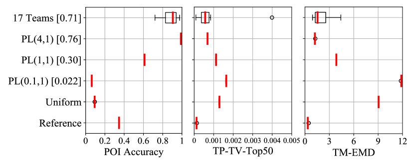
Figure 13. Box plots of $17$ points (utility values of the $17$ teams). The number in the square bracket represents the average utility score $s_{U}^{(t)}$. The red line represents the median. The variance is very small for PL, Uniform, and Reference because the same obfuscation method is used for all of the original traces. Higher is better for POI Accuracy. Lower is better for the others.

Figure 13 shows that 17 Teams and PL($4,1$) (both of which satisfy $s_{U}^{(t)}>0.7$) provide very high utility for POI Accuracy (the median is $0.9$ or more). This is because the POI recommendation task explained above requires each location in the anonymized trace to be close to the corresponding location in the original trace. Since the utility score in our contest is based on this requirement, it is inherently suitable for POI recommendation based on anonymized traces. Figure 13 also shows that the POI accuracy of Reference is low. This means that preserving only statistical information of the original traces is not sufficient for POI recommendation.

Figure 13 also shows that 17 Teams and PL($4,1$) provide almost the same performance as Reference for TP-TV-Top50 and TM-EMD, which means that statistical information is also well preserved when $s_{U}^{(t)}>0.7$. Therefore, our utility score can be used as a simple guideline to achieve high utility in geo-data analysis.

In summary, the valid anonymized traces are useful for various applications, including POI recommendation and geo-data analysis (e.g., mining popular POIs, modeling human mobility patterns).

6. Conclusion

We designed and held a location trace anonymization contest that deals with a long trace and fine-grained locations. We showed through the contest that an anonymization method secure against trace inference is also secure against re-identification in a situation where both defense and attack compete together. We also showed that the anonymized traces in our contest are useful for various applications including POI recommendation and geo-data analysis.

Appendix A Location Synthesizer for a Contest

Below, we explain the details of our location synthesizer. Our location synthesizer extends the location synthesizer in (Murakami et al., 2021) called privacy-preserving multiple tensor factorization (PPMTF) to have diversity. Therefore, we denote our location synthesizer by PPMTF+. We first briefly review PPMTF (the part most relevant to our location synthesizer). Then, we explain how our location synthesizer PPMTF+ extends PPMTF to have diversity.

PPMTF.  PPMTF trains a feature vector of each training user from training traces and generates a synthetic trace from the feature vector. Let $n\in\mathbb{N}$ be the number of training users and $z\in\mathbb{N}$ be the dimension of the feature vector. Let $\mathbf{A}\in\mathbb{R}^{n\times z}$ be the feature vectors of all training users, and $\mathbf{a}_{i}\in\mathbb{R}^{z}$ be the $i$-th row of $\mathbf{A}$. $\mathbf{a}_{i}$ represents a feature vector of the $i$-th training user. Each column in $\mathbf{A}$ represents a cluster of users, such as “those who go to a bar at night” and “those who go to a park at noon.” For example, assume that the first column of $\mathbf{A}$ represents a cluster of users who go to a bar at night. Then, a user who has a large value in the first element of her feature vector $\mathbf{a}_{i}$ tends to go to bar at night in her trace. PPMTF automatically finds such user clusters ($z$ clusters in total) from training traces.

More specifically, PPMTF trains feature vectors and generates traces as follows. First, PPMTF assumes that each feature vector is independently generated from a multivariate normal distribution:

(3) $$p(\mathbf{A}|\Psi_{\mathbf{A}}) =\textstyle\prod_{i=1}^{n}\mathcal{N}(\mathbf{a}_{i}|\mu_{\mathbf{A}},\Lambda_{\mathbf{A}}^{\!-1}),$$

where $\mu_{\mathbf{A}}\in\mathbb{R}^{z}$ is a mean vector and $\Lambda_{\mathbf{A}}\in\mathbb{R}^{z\times z}$ is a precision (inverse covariance) matrix. $\mathcal{N}(\mathbf{a}_{i}|\mu_{\mathbf{A}},\Lambda_{\mathbf{A}}^{\!-1})$ denotes the probability of $\mathbf{a}_{i}$ in the normal distribution with mean vector $\mu_{\mathbf{A}}$ and covariance matrix $\Lambda_{\mathbf{A}}^{\!-1}$. Let $\Psi_{\mathbf{A}}=(\mu_{\mathbf{A}},\Lambda_{\mathbf{A}})$. $\Psi_{\mathbf{A}}$ forms a feature vector distribution. PPMTF trains $\Psi_{\mathbf{A}}$ from training traces via posterior sampling (Wang et al., 2015), which samples a parameter from its posterior distribution given training data. Then, PPMTF trains $\mathbf{A}$ based on $\Psi_{\mathbf{A}}$ and training traces. Finally, PPMTF generates a synthetic trace that resembles the $i$-th training user’s trace based on $\mathbf{a}_{i}$.

PPMTF provides high utility in that it preserves various statistical features of training traces such as a distribution of visit-fractions (Do and Gatica-Perez, 2013; Ye et al., 2011), time-dependent population distribution (Zheng et al., 2009), and transition matrix (Liu et al., 2013; Song et al., 2006). PPMTF also protects privacy of training users. Specifically, the authors in (Murakami et al., 2021) show through experiments that the synthetic traces are secure against re-identification attacks (Gambs et al., 2014; Mulder et al., 2008; Murakami, 2017; Shokri et al., 2011) and membership inference attacks (Jayaraman and Evans, 2019; Shokri et al., 2017). See (Murakami et al., 2021) for more details of PPMTF.

Our Location Synthesizer PPMTF+.  After training $\Psi_{\mathbf{A}}$ and $\mathbf{A}$ from training traces, PPMTF generates traces from $\mathbf{A}$. In contrast, our location synthesizer PPMTF+ discards $\mathbf{A}$ and randomly samples new feature vectors from $\Psi_{\mathbf{A}}$.

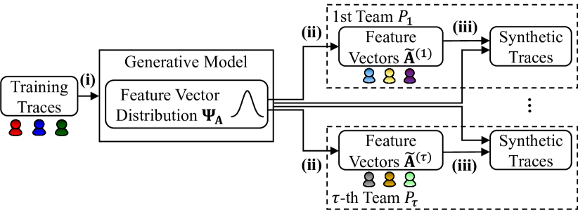
Figure 14. Our location synthesizer PPMTF+. It consists of the following three steps: (i) training a generative model, (ii) sampling new feature vectors, and (iii) generating synthetic traces.

Figure 14 shows our synthesizer PPMTF+. The number $m$ of virtual users can be different from the number $n$ of training users. We first train a generative model in the same way as PPMTF. Then, we randomly sample a new matrix $\tilde{\mathbf{A}}^{(t)}\in\mathbb{R}^{m\times z}$ ($m$ feature vectors) for team $P_{t}$ from $\Psi_{\mathbf{A}}$. Specifically, let $\tilde{\mathbf{a}}_{i}^{(t)}\in\mathbb{R}^{z}$ be the $i$-th row of $\tilde{\mathbf{A}}^{(t)}$, i.e., the $i$-th virtual user’s feature vector in team $P_{t}$. We randomly sample $\tilde{\mathbf{a}}_{i}^{(t)}$ as follows:

(4) $$\tilde{\mathbf{a}}_{i}^{(t)}\sim\mathcal{N}(\cdot|\mu_{\mathbf{A}},\Lambda_{\mathbf{A}}^{\!-1}),$$

where $\mathcal{N}(\cdot|\mu_{\mathbf{A}},\Lambda_{\mathbf{A}}^{\!-1})$ denotes the normal distribution with mean vector $\mu_{\mathbf{A}}$ and covariance matrix $\Lambda_{\mathbf{A}}^{\!-1}$. Note that we do not use training traces in (4). PPMTF trains $\mathbf{A}$ based on $\Psi_{\mathbf{A}}$ and training traces so that $\mathbf{A}$ preserves the feature of training users. In contrast, we randomly sample $\tilde{\mathbf{a}}_{i}^{(t)}$ based on $\Psi_{\mathbf{A}}$, independently of training traces. After sampling $\tilde{\mathbf{A}}^{(t)}$, we generate synthetic traces by replacing $\mathbf{A}$ with $\tilde{\mathbf{A}}^{(t)}$ in PPMTF (see (Murakami et al., 2021) for how to generate synthetic traces from the generative model in PPMTF).

Since each feature vector $\tilde{\mathbf{a}}_{i}^{(t)}$ is independently and randomly sampled, each virtual user has a different feature vector than the training users and the other virtual users. This yields the diversity. In addition, both $\mathbf{a}_{i}$ and $\tilde{\mathbf{a}}_{i}^{(t)}$ follow the normal distribution with parameter $\Psi_{\mathbf{A}}=(\mu_{\mathbf{A}},\Lambda_{\mathbf{A}})$ (see (3) and (4)). Thus, $\tilde{\mathbf{A}}^{(t)}$ preserves very similar statistical features to $\mathbf{A}$. Consequently, our synthetic traces provide high utility in terms of various statistical features in the same way as PPMTF.

Our synthesizer PPMTF+ is also as scalable as PPMTF because sampling $\tilde{\mathbf{A}}^{(t)}$ takes little time, e.g., much less than one second even using a laptop. For example, PPMTF+ can synthesize traces of about $200000$ users within one day in the same way as PPMTF (Murakami et al., 2021).

Remark.  In our contest, we kept the algorithm of our synthesizer secret from all teams. However, we argue that a contest would be interesting even if the algorithm is made public. Specifically, if each team $P_{t}$ keeps feature vectors $\tilde{\mathbf{A}}^{(t)}$ private, the other teams cannot obtain information on how each virtual user in team $P_{t}$ behaves; e.g., some may often go to restaurants, and others may commute by train. Thus, both attacks and defenses are still very challenging and interesting.

Appendix B Diversity and Utility of Our Synthesizers

B.1. Experimental Set-up

Dataset.  We evaluated the diversity and utility of PPMTF+ in Appendix A using the Foursquare dataset in (Yang et al., 2019). Following (Yang et al., 2019), we selected six cities with many check-ins and with cultural diversity: Istanbul (IST), Jakarta (JK), New York City (NYC), Kuala Lumpur (KL), San Paulo (SP), and Tokyo (TKY).

For each city, we selected $1000$ popular POIs for which the number of visits from all users was the largest. Thus, the number of locations is $1000$ in our experiments. We set the time interval between two temporally-continuous events to one hour by rounding down minutes. Then we set a time slot (Murakami et al., 2021), a time resolution at which we want to preserve a population distribution of training traces, to two hours, i.e., $12$ time slots in total. For each city, we randomly selected $80\%$ of users as training users and used the remaining users as testing users. The traces of testing users were used for evaluating a baseline (the utility of real traces). The numbers of training users in IST, JK, NYC, KL, SP, and TKY were $n=219793$, $83325$, $52432$, $51189$, $42100$, and $32056$, respectively.

Synthesizers.  We generated synthetic traces using PPMTF+. We set the dimension $z$ of the feature vector to $z=16$ (in the same way as (Murakami et al., 2021)) and the number $\tau$ of teams to $\tau=2$. Then we generated the same number of virtual users’ feature vectors as training users ($m=n$). For each virtual user, we generated one synthetic trace with the length of $20$ days.

For comparison, we generated the same amount of synthetic traces using PPMTF (Murakami et al., 2021). As another baseline, we also evaluated the synthetic data generator (denoted by SGD) in (Bindschaedler et al., 2017). Specifically, we first calculated a transition matrix for each time slot ($12\times 1000\times 1000$ elements in total) from training traces via maximum likelihood estimation. Then we generated synthetic traces by randomly sampling locations using the transition matrix. This method is a special case of the synthetic data generator in (Bindschaedler et al., 2017) where the generative model is independent of the input data record (see (Murakami et al., 2021) for details).

SGD generates traces only based on parameters common to all users. Therefore, it does not preserve user-specific features, as shown in our experiments. Note that the user-specific features are necessary for an anonymization contest, because otherwise the adversary cannot re-identify traces. In other words, the adversary needs some user-specific features as background knowledge to re-identify traces. We do not evaluate other synthesizers such as (Chen et al., 2012a, b; He et al., 2015), because they also generate traces only based on parameters common to all users and have the same issue.

We also note that a location synthesizer in (Bindschaedler and Shokri, 2016) lacks scalability and cannot be applied to the Foursquare dataset; e.g., it requires over four years to generate traces in IST even using a supercomputer (Murakami et al., 2021).

Diversity Metrics.  For diversity, we evaluated whether the $i$-th synthetic trace for the 1st team is similar to the $i$-th synthetic trace for the 2nd team.

Specifically, we first randomly selected $2000$ virtual users from $m$ virtual users. Without loss of generality, we denote the selected user IDs by $1,\cdots,2000$. We calculated a population distribution ($1000$-dim vector) for each virtual user. Then we evaluated the average total variance between the distribution of the $i$-th user in the first team and that of the $i$-th (resp. $(1000+i)$-th) user in the second team ($1\leq i\leq 1000$), which is denoted by Same-TV (resp. Diff-TV). If Same-TV is smaller than Diff-TV, the synthesizer lacks diversity.

Note that PPMTF+ clearly has diversity because it independently and randomly samples each feature vector by (4). The purpose here is to quantitatively show that PPMTF lacks diversity.

Utility Metrics.  For utility, we evaluated a distribution of visit-fractions, time-dependent population distribution, and transition matrix in the same way as (Murakami et al., 2021).

The distribution of visit-fractions is a key feature for auto-tagging POI categories (e.g., restaurants, hotels) (Do and Gatica-Perez, 2013; Ye et al., 2011). For example, many people spend $60\%$ of the time at home and $20\%$ of the time at work/school (Do and Gatica-Perez, 2013). To evaluate such a feature, we did the following. For each training user, we computed a fraction of visits for each POI. Then we computed a distribution of visit-fractions for each POI by dividing the fraction into $24$ bins: $(0,\frac{1}{24}],(\frac{1}{24},\frac{2}{24}],\cdots,(\frac{23}{24},1)$. Figure 15 shows an example of calculating a distribution of visit-fractions for each of POIs $x_{1}$ (office) and $x_{2}$ (bar). In this example, the fraction is divided into bins with a length of $0.2$, and people tend to stay in $x_{1}$ (office) longer than $x_{2}$ (bar).

We computed a distribution of visit-fractions for each POI from synthetic traces in the same way. Finally, we evaluated the total variance between the two distributions for each POI and took the average over all POIs (denoted by VF-TV).

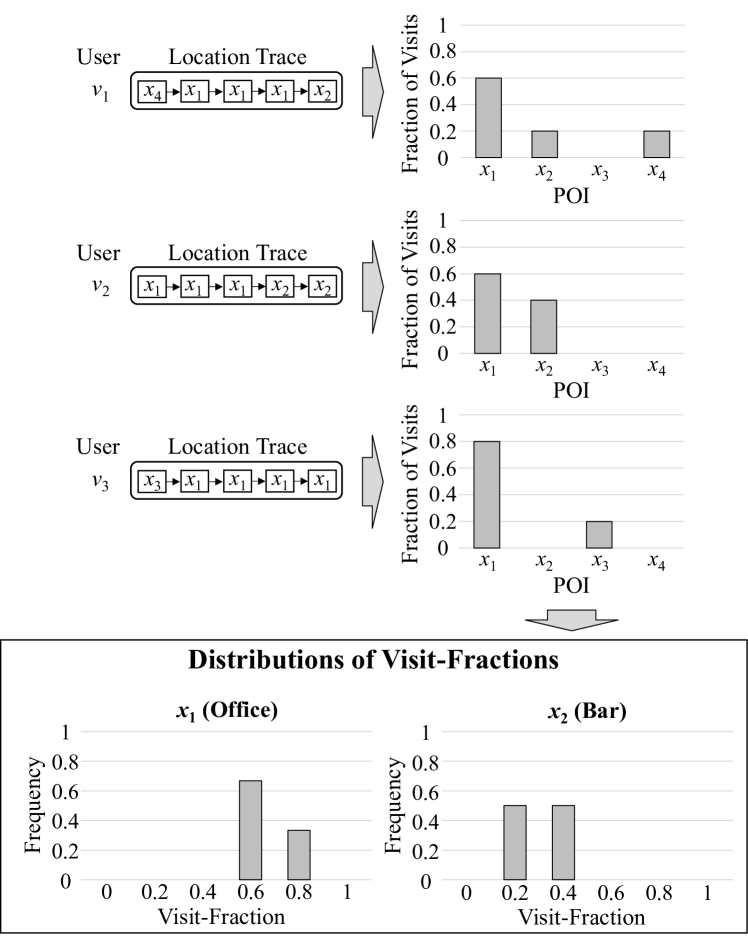
Figure 15. Example of calculating a distribution of visit-fractions from location traces.

For the population distribution and the transition matrix, we evaluated TP-TV-Top50 and TM-EMD in Section 5.5, respectively.

B.2. Experimental Results

Diversity.  We first evaluated the diversity of PPMTF+ and PPMTF. Figure 17 shows the results. In PPMTF, Same-TV is smaller than Diff-TV, which means that the $i$-th synthetic trace for the 1st team is similar to the $i$-th synthetic trace for the 2nd team. Thus, PPMTF lacks diversity. In contrast, Same-TV is almost the same as Diff-TV (their difference is much smaller than $0.1$ times the standard deviation) in PPMTF+. This is because PPMTF+ independently samples each feature vector.

Utility.  We next evaluated the utility. Figure 17 shows the results. Here, we evaluated each utility metric for each of $20$ days in the 1st team and averaged it over $20$ days. Uniform is the utility when all locations in synthetic traces are independently sampled from a uniform distribution. Real is the utility of the traces of testing users, i.e., real traces. Ideally, the utility of synthetic traces should be much better (smaller) than that of Uniform and close to that of Real.

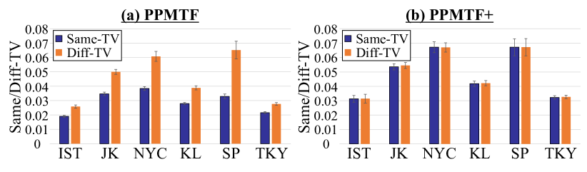
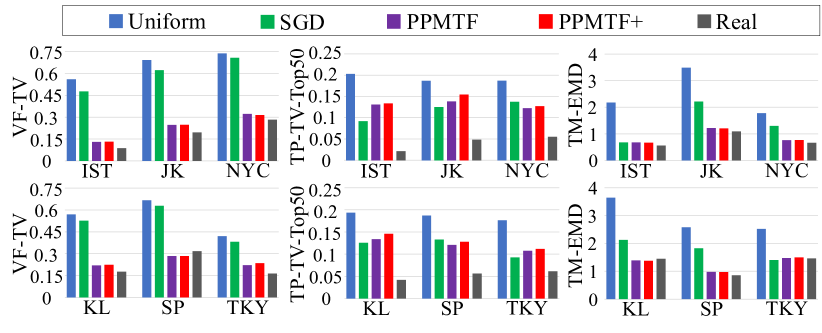
Figure 16. Diversity of PPMTF and PPMTF+. The error bar shows $0.1\times$ the standard deviation over $1000$ pairs of users.

Figure 17. Utility of each location synthesizer. Lower is better in all metrics.

Figure 17 shows that SGD provides poor utility (almost the same as Uniform) in terms of VF-TV. This is because SGD generates traces using parameters common to all users. Consequently, all users spend almost the same amount of time on each POI. In other words, SGD cannot preserve user-specific features. As explained above, the user-specific features are necessary for re-identification in an anonymization contest.

In contrast, PPMTF+ provides high utility in all utility metrics in the same way as PPMTF. This is because feature vectors $\tilde{\mathbf{A}}^{(t)}$ in PPMTF+ preserve very similar statistical features to feature vectors $\mathbf{A}$ in PPMTF.

Summary.  In summary, the existing synthesizers lack either diversity or user-specific features. Thus, they cannot be applied to an anonymization contest in the partial-knowledge attacker model. In contrast, PPMTF+ provides both diversity and utility including user-specific features. Thus, it fulfills the need for our contest.

Appendix C Privacy of Our Synthesizer

Experimental Set-up.  To evaluate the privacy of PPMTF+ in Appendix A, we used the SNS-based people flow data (Nightley and Center for Spatial Information Science at the University of Tokyo (2014), CSIS) (Tokyo) and processed the data in the same way as (Murakami et al., 2021). There were $400$ regions and $n=500$ training users (see (Murakami et al., 2021) for details). We generated synthetic traces using our location synthesizer PPMTF+ with $z=16$ and $\tau=1$. We generated synthetic traces of virtual users of the same number as the training users ($m=n$). For each virtual user, we generated one synthetic trace with a length of ten days.

For comparison, we also generated the same amount of synthetic traces using PPMTF. Since we used a relatively small dataset ($n=500$) in this experiment, we also evaluated the synthetic location traces generator in (Bindschaedler and Shokri, 2016) (denoted by SGLT). We used the SGLT tool in (Bindschaedler and Shokri, 2016). We set the number $c$ to semantic clusters to $c=50$ or $100$ because they provided the best performance. We set the other parameters in the same way as (Murakami et al., 2021).

For utility, we evaluated TP-TV-Top50 and TM-EMD in Section B. We did not evaluate VF-TV, a utility measure for auto-tagging POI categories, because we used regions rather than POIs in this experiment.

For privacy, we considered two privacy attacks: re-identification (or de-anonymization) attack (Gambs et al., 2014; Mulder et al., 2008; Murakami, 2017; Shokri et al., 2011) and membership inference attack (Jayaraman and Evans, 2019; Shokri et al., 2017). For the re-identification attack, we evaluated a re-identification rate. For the membership inference attack, we used the membership advantage (Jayaraman and Evans, 2019; Yeom et al., 2018), the difference between the true positive rate and the false positive rate, as a privacy metric. We used the implementation of these attacks in (Murakami et al., 2021) (see (Murakami et al., 2021) for details).

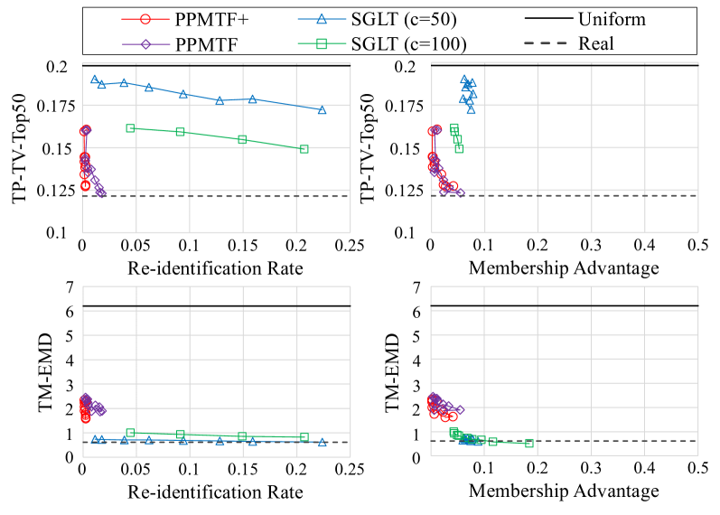
Figure 18. Privacy and utility of each location synthesizer. Lower is better in all metrics.

Results.  Figure 18 shows the results. Uniform represents the utility when all locations in synthetic traces are independently sampled from a uniform distribution. Real represents the utility of the testing traces.

Figure 18 shows that PPMTF+ achieves almost the same re-identification rate as a random guess ($=0.002$). This is because PPMTF+ independently and randomly generates each virtual user from a distribution of user profiles. In other words, the virtual users are different from the training users, i.e., diversity. Figure 18 also shows that PPMTF+ achieves almost the same membership advantage as PPMTF.

Note that TM-EMD of PPMTF+ is worse than that of SGLT. This is because PPMTF, on which PPMTF+ is based, modifies the transition matrix of each training user via the Metropolis-Hastings algorithm (see (Murakami et al., 2021) for details). However, TM-EMD of PPMTF+ is still much lower than that of Uniform, which means that PPMTF+ preserves the transition matrix well.

In summary, our experimental results show that PPMTF+ achieves the same re-identification rate as a random guess and also has security against membership inference attacks in the same way as PPMTF. Providing strong privacy guarantees such as DP (Dwork, 2006; Dwork and Roth, 2014) is left for future work.

Appendix D Generation of Home Regions

In our contest, we slightly modified PPMTF+ in Appendix A so that each virtual user has her own home.

We first extracted training traces from 6:00 to 18:00 for $10181$ users who have at least $10$ locations from the SNS-based people flow data. We trained our generative model from these training traces and sampled feature vectors of $m=2000$ virtual users in PPMTF+. Then, we randomly selected a home region for each virtual user from a population distribution at 6:00. PPMTF+ generates a synthetic trace of each user using a visit-count matrix, which includes a visit-count for each region and each time slot (see (Murakami et al., 2021) for details). Thus, we increased visit-counts of the virtual user in her home region from 6:00 to 8:00 and 16:00 to 18:00 so that she stays at home in the morning and evening with high probability. After that, we generated a synthetic trace from 6:00 to 18:00 for 40 days for each virtual user using this modified synthesizer.

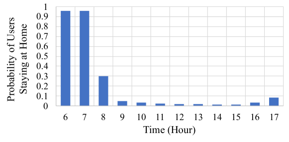
Figure 19. Probability of users staying at home.

Figure 19 shows the probability of users staying at a home region. We also show in Figure 4 the population distribution of the synthetic traces in our contest at 12:00. These figures show that synthetic traces are generated so that each user stays at home in the morning and evening with high probability, while keeping the time-dependent population distribution of the training traces. We have also confirmed that our synthetic traces preserve the transition matrix of the training traces.

After the generation of synthetic traces, we extracted locations from 8:00 to 18:00 in 30-minute intervals for each of 40 days and used them for our contest. Note that almost all virtual users stay at home from 6:00 to 8:00, as shown in Figure 19. Thus, if we include locations from 6:00 to 8:00 in reference traces, the adversary would know home regions of almost all virtual users. Because this is too informative for the adversary, we excluded locations from 6:00 to 8:00 in our contest.

Appendix E Fairness in Our Contest

We evaluated the fairness of our contest by calculating the variance of privacy scores as follows. We anonymized the original traces of the $17$ teams using No Obfuscation, MRLH($1,1,0.5$), RR($1$), or PL($1,1$). Then we applied all the sample attack algorithms to the anonymized traces and evaluated the standard deviation (SD) of the privacy scores $s_{R,min}^{(t)}$ and $s_{T,min}^{(t)}$.

Table 2 shows the results. The SD is very small when we apply RR($1$). This is because RR($1$) rarely outputs the original region (with probability $0.0027$). The SD is the largest when we do not apply any obfuscation algorithms (No Obfuscation), in which case the SD is about $0.01$.

Table 2. Standard deviation (SD) of the minimum privacy scores $s_{R,min}^{(t)}$ and $s_{T,min}^{(t)}$ for the $17$ teams calculated by the sample anonymization and attack algorithms (NO: No Obfuscation).

NO MRLH($1,1,0.5$) RR($1$) PL($1,1$) $s_{R,min}^{(t)}$ $0.0095$ $0.0068$ $0.00055$ $0.0026$ $s_{T,min}^{(t)}$ $0.011$ $0.0033$ $0.00015$ $0.0010$

Table 2 and Figure 9 show that for re-identification, the standard deviation ($=0.01$) is much smaller than the difference between the best privacy score ($=0.79$) and the second-best privacy score ($=0.67$). Thus, it is highly unlikely that the difference of the original traces changes the order of the 1st and 2nd places. For trace inference, the best, second-best, and third-best privacy scores are $0.720$, $0.709$, and $0.637$, respectively. Thus, the difference of the original traces may affect the order of the 1st and 2nd places. However, it is highly unlikely that the difference of the original traces changes the order of the 2nd and 3rd places.

To improve the fairness (i.e., to further reduce the SD), we should increase the number $m$ of virtual users. However, the increase of $m$ would increase the burden of each team during the contest. We should consider both the fairness and the burden of each team when we decide a value of $m$.

Appendix F Examples of Sample Attack Algorithms

The upper panel of Figure 20 shows examples of visit probability vectors. Here, we assign a very small positive value $\delta$ ($=10^{-8}$) to an element with zero probability. The middle panel of Figure 20 shows an example of VisitProb-R. In this example, “user ID = 3” is output as a re-identification result, as it achieves the highest likelihood. The lower panel of Figure 20 shows an example of VisitProb-T. For perturbation, it outputs the noisy location as is. For generalization (marked with blue), it randomly chooses a region from generalized regions. For deletion (marked with red), it randomly chooses a region from all regions.

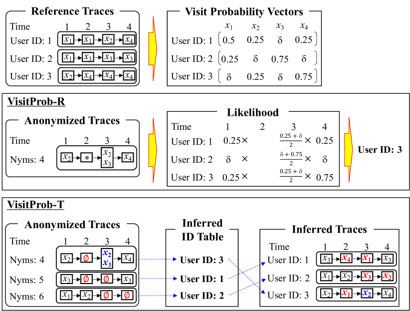
Figure 20. Examples of visit probability vectors, VisitProb-R, and VisitProb-T.

References

- (1)
- PWS (2019) 2019. PWS Cup 2019. https://www.iwsec.org/pws/2019/cup19_e.html.
- Loc (2022) 2022. Tool: PPMTF+. https://github.com/PPMTFPlus/PPMTFPlus.
- Aggarwal and Yu (2008) Charu C. Aggarwal and Philip S. Yu. 2008. Privacy-Preserving Data Mining. Springer.
- Andrés et al. (2013) Miguel E. Andrés, Nicolás E. Bordenabe, Konstantinos Chatzikokolakis, and Catuscia Palamidessi. 2013. Geo-Indistinguishability: Differential Privacy for Location-based Systems. In Proceedings of the 20th ACM Conference on Computer and Communications Security (CCS’13). 901–914.
- Bergstra and Bengio (2012) James Bergstra and Yoshua Bengio. 2012. Journal of Machine Learning Research. Random Search for Hyper-Parameter Optimization 13, 10 (2012), 281–305.
- Bettini et al. (2009) Claudio Bettini, Sushil Jajodia, Pierangela Samarati, and Sean X. Wang. 2009. Privacy in Location-Based Applications: Research Issues and Emerging Trends. Springer.
- Bettini et al. (2005) Claudio Bettini, X. Sean Wang, and Sushil Jajodia. 2005. Protecting Privacy against Location-based Personal Identification. In Proceedings of the 2nd VLDB Workshop on Secure Data Management (SDM’05). 185–199.
- Bilogrevic et al. (2013) Igor Bilogrevic, Kévin Huguenin, Murtuza Jadliwala, Florent Lopez, Jean-Pierre Hubaux, Philip Ginzboorg, and Valtteri Niemi. 2013. Inferring Social Ties in Academic Networks Using Short-range Wireless Communications. In Proceedings of the 12th ACM Workshop on Privacy in the Electronic Society (WPES’13). 179–188.
- Bindschaedler et al. (2012) Laurent Bindschaedler, Murtuza Jadliwala, Igor Bilogrevic, Imad Aad, Philip Ginzboorg, Valtteri Niemi, and Jean-Pierre Hubaux. 2012. Track Me If You Can: On the Effectiveness of Context-based Identifier Changes in Deployed Mobile Networks. In Proceedings of the 19th Network and Distributed System Security Symposium (NDSS’12). 1–17.
- Bindschaedler and Shokri (2016) Vincent Bindschaedler and Reza Shokri. 2016. Synthesizing Plausible Privacy-preserving Location Traces. In Proceedings of the 2016 IEEE Symposium on Security and Privacy (S&P’16). 546–563.
- Bindschaedler et al. (2017) Vincent Bindschaedler, Reza Shokri, and Carl A. Gunter. 2017. Plausible Deniability for Privacy-preserving Data Synthesis. Proceedings of the VLDB Endowment 10, 5 (2017), 481–492.
- Bonneel et al. (2015) Nicolas Bonneel, Julien Rabin, Gabriel Peyré, and Hanspeter Pfister. 2015. Sliced and Radon Wasserstein Barycenters of Measures. Journal of Mathematical Imaging and Vision 51, 1 (2015), 22–45.
- Bordenabe et al. (2014) Nicolas E. Bordenabe, Konstantinos Chatzikokolakis, and Catuscia Palamidessi. 2014. Optimal Geo-Indistinguishable Mechanisms for Location Privacy. In Proceedings of the 21st ACM Conference on Computer and Communications Security (CCS’14). 251–262.
- Chen et al. (2012a) Rui Chen, Gergely Acs, and Claude Castelluccia. 2012a. Differentially Private Sequential Data Publication via Variable-Length N-Grams. In Proceedings of the 19th ACM Conference on Computer and Communications Security (CCS’12). 638–649.
- Chen et al. (2012b) Rui Chen, Benjamin C. M. Fung, Bipin C. Desai, and Nériah M. Sossou. 2012b. Differentially Private Transit Data Publication: A Case Study on the Montreal Transportation System. In Proceedings of the 18th ACM SIGKDD International Conference on Knowledge Discovery and Data Mining (KDD’12). 213–221.
- Cheng et al. (2013) Chen Cheng, Haiqin Yang, Michael R. Lyu, and Irwin King. 2013. Where You Like to Go Next: Successive Point-of-Interest Recommendation. In Proceedings of the 23rd International Joint Conference on Artificial Intelligence (IJCAI’13). 2605–2611.
- Cho et al. (2011) Eunjoon Cho, Seth A. Myers, and Jure Leskovec. 2011. Friendship and Mobility: User Movement in Location-based Social Networks. In Proceedings of the 17th ACM SIGKDD International Conference on Knowledge Discovery and Data Mining (KDD’11). 1082–1090.
- Chow and Mokbel (2011) Chi-Yin Chow and Mohamed F. Mokbel. 2011. Trajectory Privacy in Location-based Services and Data Publication. ACM SIGKDD Explorations Newsletter 13, 1 (2011), 19–29.
- Chow and Golle (2009) Richard Chow and Philippe Golle. 2009. Faking Contextual Data for Fun, Profit, and Privacy. In Proceedings of the 8th ACM Workshop on Privacy in the Electronic Society (WPES’09). 105–108.
- de Montjoye et al. (2013) Yves-Alexandre de Montjoye, César A. Hidalgo, Michel Verleysen, and Vincent D. Blondel. 2013. Unique in the Crowd: The privacy bounds of human mobility. Scientific Reports 3, 1376 (2013), 1–5.
- Desfontaines and Pejó (2020) Damien Desfontaines and Balázs Pejó. 2020. SoK: Differential Privacies. Proceedings on Privacy Enhancing Technologies (PoPETs) 2 (2020), 288–313.
- Do and Gatica-Perez (2013) Trinh Minh Tri Do and Daniel Gatica-Perez. 2013. The Places of Our Lives: Visiting Patterns and Automatic Labeling from Longitudinal Smartphone Data. IEEE Transactions on Mobile Computing 13, 3 (2013), 638–648.
- Domingo-Ferrer et al. (2015) Josep Domingo-Ferrer, Sara Ricci, and Jordi Soria-Comas. 2015. Disclosure Risk Assessment via Record Linkage by a Maximum-Knowledge Attacker. In Proceedings of the 13th Annual Conference on Privacy, Security and Trust (PST’15). 3469–3478.
- Dwork (2006) Cynthia Dwork. 2006. Differential Privacy. In Proceedings of the 33rd international conference on Automata, Languages and Programming (ICALP’06). 1–12.
- Dwork and Roth (2014) Cynthia Dwork and Aaron Roth. 2014. The Algorithmic Foundations of Differential Privacy. Now Publishers.
- Eagle et al. (2009) Nathan Eagle, Alex Pentland, and David Lazer. 2009. Inferring Friendship Network Structure by Using Mobile Phone Data. Proceedings of the National Academy of Sciences (PNAS) 106, 36 (2009), 15274–15278.
- Elsken et al. (2019) Thomas Elsken, Jan Hendrik Metzen, and Frank Hutter. 2019. Journal of Machine Learning Research. Neural Architecture Search: A Survey 20, 1 (2019), 1997–2017.
- Feng et al. (2015) Shanshan Feng, Xutao Li, Yifeng Zeng, Gao Cong, Yeow Meng Chee, and Quan Yuan. 2015. Personalized Ranking Metric Embedding for Next New POI Recommendation. In Proceedings of the 24th International Joint Conference on Artificial Intelligence (IJCAI’15). 2069–2075.
- Gambs et al. (2014) Sébastien Gambs, Marc-Olivier Killijian, and Miguel Núñez del Prado Cortez. 2014. De-anonymization Attack on Geolocated Data. J. Comput. System Sci. 80, 8 (2014), 1597–1614.
- Garfinkel (2015) Simon L. Garfinkel. 2015. NISTIR 8053: De-Identification of Personal Information. Technical Report. National Institute of Standards and Technology.
- Gedik and Liu (2008) Buğra Gedik and Ling Liu. 2008. Protecting Location Privacy with Personalized k-Anonymity: Architecture and Algorithms. IEEE Transactions on Mobile Computing 7, 1 (2008), 1–18.
- He et al. (2015) Xi He, Graham Cormode, Ashwin Machanavajjhala, Cecilia M. Procopiuc, and Divesh Srivastava. 2015. DPT: Differentially Private Trajectory Synthesis Using Hierarchical Reference Systems. Proceedings of the VLDB Endowment 11, 8 (2015), 1154–1165.
- Jayaraman and Evans (2019) Bargav Jayaraman and David Evans. 2019. Evaluating Differentially Private Machine Learning in Practice. In Proceedings of the 28th USENIX Security Symposium (USENIX Security’19). 1895–1912.
- Jordon et al. (2020) James Jordon, Daniel Jarrett, Jinsung Yoon, Tavian Barnes, Paul Elbers, Patrick Thoral, Ari Ercole, Cheng Zhang, Danielle Belgrave, and Mihaela van der Schaar. 2020. Hide-and-Seek Privacy Challenge. CoRR 2007.12087 (2020). https://arxiv.org/abs/2007.12087
- Kairouz et al. (2016) Peter Kairouz, Keith Bonawitz, and Daniel Ramage. 2016. Discrete Distribution Estimation under Local Privacy. In Proceedings of the 33rd International Conference on Machine Learning (ICML’16). 2436–2444.
- Kido et al. (2005) Hidetoshi Kido, Yutaka Yanagisawa, and Tetsuji Satoh. 2005. An Anonymous Communication Technique Using Dummies for Location-based Services. Proceedings of the 2005 IEEE International Conference on Pervasive Services (ICPS’05) (2005), 88–97.
- Kikuchi et al. (2016a) Hiroaki Kikuchi, Takayasu Yamaguchi, Koki Hamada, Yuji Yamaoka, Hidenobu Oguri, and Jun Sakuma. 2016a. Ice and Fire: Quantifying the Risk of Re-identification and Utility in Data Anonymization. In Proceedings of 2016 IEEE 30th International Conference on Advanced Information Networking and Applications (AINA’16). 1035–1042.
- Kikuchi et al. (2016b) Hiroaki Kikuchi, Takayasu Yamaguchi, Koki Hamada, Yuji Yamaoka, Hidenobu Oguri, and Jun Sakuma. 2016b. A Study from the Data Anonymization Competition Pwscup 2015. In Proceedings of the 11th International Workshop, DPM 2016 and 5th International Workshop, QASA 2016 (DPM/QASA’16). 230–237.
- Kolouri et al. (2018) Soheil Kolouri, Gustavo K. Rohde, and Heiko Hoffmann. 2018. SlicedWasserstein Distance for Learning Gaussian Mixture Models. In Proceedings of the 2018 IEEE/CVF Conference on Computer Vision and Pattern Recognition (CVPR’18). 3427–3436.
- Li et al. (2016) Ninghui Li, Min Lyu, and Dong Su. 2016. Differential Privacy: From Theory to Practice. Morgan & Claypool Publishers.
- Liu et al. (2013) Xin Liu, Yong Liu, Karl Aberer, and Chunyan Miao. 2013. Personalized Point-of-Interest Recommendation by Mining Users’ Preference Transition. In Proceedings of the 22nd ACM international conference on Information & Knowledge Management (CIKM’13). 733–738.
- Liu et al. (2017) Yiding Liu, Tuan-Anh Nguyen Pham, Gao Cong, and Quan Yuan. 2017. An Experimental Evaluation of Point-of-interest Recommendation in Location-based Social Networks. Proceedings of the VLDB Endowment 10, 10 (2017), 1010–1021.
- Machanavajjhala et al. (2006) Ashwin Machanavajjhala, Johannes Gehrke, Daniel Kifer, and Muthuramakrishnan Venkitasubramaniam. 2006. l-diversity: Privacy beyond k-anonymity. In Proceedings of the 22nd International Conference on Data Engineering (ICDE’06). 24–35.
- Maldoff (2016) Gabe Maldoff. 2016. Top 10 Operational Impacts of the GDPR: Part 8 - Pseudonymization. https://iapp.org/news/a/top-10-operational-impacts-of-the-gdpr-part-8-pseudonymization/.
- Meehan and Chaudhuri (2021) Casey Meehan and Kamalika Chaudhuri. 2021. Location Trace Privacy under Conditional Priors. In Proceedings of the 24th International Conference on Artificial Intelligence and Statistics (AISTATS’21). 2881–2889.
- Mulder et al. (2008) Yoni De Mulder, George Danezis, Lejla Batina, and Bart Preneel. 2008. Identification via Location-profiling in GSM Networks. In Proceedings of the 7th ACM Workshop on Privacy in the Electronic Society (WPES’08). 23–32.
- Murakami (2017) Takao Murakami. 2017. Expectation-Maximization Tensor Factorization for Practical Location Privacy Attacks. Proceedings on Privacy Enhancing Technologies (PoPETs) 4 (2017), 138–155.
- Murakami et al. (2021) Takao Murakami, Koki Hamada, Yusuke Kawamoto, and Takuma Hatano. 2021. Privacy-Preserving Multiple Tensor Factorization for Synthesizing Large-Scale Location Traces with Cluster-Specific Features. Proceedings on Privacy Enhancing Technologies (PoPETs) 2 (2021), 5–26.
- Murakami et al. (2017) Takao Murakami, Atsunori Kanemura, and Hideitsu Hino. 2017. Group Sparsity Tensor Factorization for Re-identification of Open Mobility Traces. IEEE Transactions on Information Forensics and Security 12, 3 (2017), 689–704.
- Murakami and Takahashi (2021) Takao Murakami and Kenta Takahashi. 2021. Transactions on Data Privacy. Toward Evaluating Re-identification Risks in the Local Privacy Model 14, 3 (2021), 79–116.
- Narayanan and Shmatikov (2008) Arvind Narayanan and Vitaly Shmatikov. 2008. Robust De-anonymization of Large Sparse Datasets. In Proceedings of the 2008 IEEE Symposium on Security and Privacy (S&P’08). 111–125.
- Nightley and Center for Spatial Information Science at the University of Tokyo (2014) (CSIS) Nightley and Center for Spatial Information Science at the University of Tokyo (CSIS). 2014. SNS-based People Flow Data. http://nightley.jp/archives/1954.
- NIST 2018 Differential Privacy Synthetic Data Challenge (2018) NIST 2018 Differential Privacy Synthetic Data Challenge. 2018. https://www.nist.gov/ctl/pscr/open-innovation-prize-challenges/past-prize-challenges/2018-differential-privacy-synthetic.
- NIST 2020 Differential Privacy Temporal Map Challenge (2020) NIST 2020 Differential Privacy Temporal Map Challenge. 2020. https://www.nist.gov/ctl/pscr/open-innovation-prize-challenges/current-and-upcoming-prize-challenges/2020-differential.
- Nojima et al. (2018) Ryo Nojima, Hidenobu Oguri, Hiroaki Kikuchi, Hiroshi Nakagawa, Koki Hamada, Takao Murakami, and Chiemi Watanabe. 2018. How to Handle Excessively Anonymized Datasets. Journal of Information Processing 26 (2018), 477–485.
- Pyrgelis et al. (2017) Apostolos Pyrgelis, Carmela Troncoso, and Emiliano De Cristofaro. 2017. What Does The Crowd Say About You? Evaluating Aggregation-based Location Privacy. Proceedings on Privacy Enhancing Technologies (PoPETs) 2017, 4 (2017), 76–96.
- Pyrgelis et al. (2018) Apostolos Pyrgelis, Carmela Troncoso, and Emiliano De Cristofaro. 2018. Knock Knock, Who’s There? Membership Inference on Aggregate Location Data. In Proceedings of the 25th Network and Distributed System Security Symposium (NDSS’18). 1–15.
- Re-identification — CROS - European Commission (2019) Re-identification — CROS - European Commission. 2019. https://ec.europa.eu/eurostat/cros/content/re-identification_en.
- Ruiz et al. (2018) Nicolas Ruiz, Krishnamurty Muralidhar, and Josep Domingo-Ferrer. 2018. On the Privacy Guarantees of Synthetic Data: A Reassessment from the Maximum-Knowledge Attacker Perspective. In Proceedings of the International Conference on Privacy in Statistical Databases (PSD’18). 59–74.
- Shokri et al. (2017) Reza Shokri, Marco Stronati, Congzheng Song, and Vitaly Shmatikov. 2017. Membership Inference Attacks Against Machine Learning Models. In Proceedings of the 2017 IEEE Symposium on Security and Privacy (S&P’17). 3–18.
- Shokri et al. (2011) Reza Shokri, George Theodorakopoulos, Jean-Yves Le Boudec, and Jean-Pierre Hubaux. 2011. Quantifying Location Privacy. In Proceedings of the 2011 IEEE Symposium on Security and Privacy (S&P’11). 247–262.
- Shokri et al. (2012) Reza Shokri, George Theodorakopoulos, Carmela Troncoso, Jean-Pierre Hubaux, and Jean-Yves Le Boudec. 2012. Protecting Location Privacy: Optimal Strategy against Localization Attacks. Proceedings of the 2012 ACM Conference on Computer and Communications Security (CCS’12) (2012), 617–627.
- Song et al. (2006) Libo Song, David Kotz, Ravi Jain, and Xiaoning He. 2006. Evaluating Next-cell Predictors with Extensive wi-fi Mobility Data. IEEE Transactions on Mobile Computing 5, 12 (2006), 1633–1649.
- Sweeney (2002) Latanya Sweeney. 2002. International Journal on Uncertainty, Fuzziness and Knowledge-based Systems. k-Anonymity: A Model for Protecting Privacy 10, 5 (2002), 557–570.
- The EU General Data Protection Regulation (2016) (GDPR) The EU General Data Protection Regulation (GDPR). 2016. https://eur-lex.europa.eu/eli/reg/2016/679/oj.
- Torra (2017) Vincenç Torra. 2017. Data Privacy: Foundations, New Developments and the Big Data Challenge. Springer.
- Wang et al. (2015) Yu-Xiang Wang, Stephen E. Fienberg, and Alexander J. Smola. 2015. Privacy for Free: Posterior Sampling and Stochastic Gradient Monte Carlo. In Proceedings of the 32nd International Conference on International Conference on Machine Learning (ICML’15). 2493–2502.
- Xiao and Xiong (2015) Yonghui Xiao and Li Xiong. 2015. Protecting Locations with Differential Privacy under Temporal Correlations. In Proceedings of the 22nd ACM SIGSAC Conference on Computer and Communications Security (CCS’15). 1298–1309.
- Yang et al. (2019) Dingqi Yang, Bingqing Qu, Jie Yang, and Philippe Cudre-Mauroux. 2019. Revisiting User Mobility and Social Relationships in LBSNs: A Hypergraph Embedding Approach. In Proceedings of the 2019 World Wide Web Conference (WWW’19). 2147–2157.
- Ye et al. (2011) Mao Ye, Dong Shou, Wang-Chien Lee, Peifeng Yin, and Krzysztof Janowicz. 2011. On the Semantic Annotation of Places in Location-Based Social Networks. In Proceedings of the 17th ACM SIGKDD International Conference on Knowledge Discovery and Data Mining (KDD’11). 520–528.
- Yeom et al. (2018) Samuel Yeom, Irene Giacomelli, Matt Fredrikson, and Somesh Jha. 2018. Privacy Risk in Machine Learning: Analyzing the Connection to Overfitting. In Proceedings of the 2018 IEEE 31st Computer Security Foundations Symposium (CSF’18). 268–282.
- You et al. (2007) Tun-Hao You, Wen-Chih Peng, and Wang-Chien Lee. 2007. Protecting Moving Trajectories with Dummies. In Proceedings of the 2007 International Conference on Mobile Data Management (MDM’07). 278–282.
- Zheng et al. (2010) Yu Zheng, Xing Xie, and Wei-Ying Ma. 2010. GeoLife: A Collaborative Social Networking Service among User, Location and Trajectory. IEEE Data Engineering Bulletin 32, 2 (2010), 32–40.
- Zheng et al. (2009) Yu Zheng, Lizhu Zhang, Xing Xie, and Wei-Ying Ma. 2009. Mining Interesting Locations and Travel Sequences from GPS Trajectories. In Proceedings of the 18th International Conference on World Wide Web (WWW’09). 791–800.