Species Distribution Modeling for Machine Learning Practitioners: A Review

Abstract.

Conservation science depends on an accurate understanding of what’s happening in a given ecosystem. How many species live there? What is the makeup of the population? How is that changing over time? Species Distribution Modeling (SDM) seeks to predict the spatial (and sometimes temporal) patterns of species occurrence, i.e. where a species is likely to be found. The last few years have seen a surge of interest in applying powerful machine learning tools to challenging problems in ecology (AI_, [n.d.]a, [n.d.]b; FGV, [n.d.]). Despite its considerable importance, SDM has received relatively little attention from the computer science community. Our goal in this work is to provide computer scientists with the necessary background to read the SDM literature and develop ecologically useful ML-based SDM algorithms. In particular, we introduce key SDM concepts and terminology, review standard models, discuss data availability, and highlight technical challenges and pitfalls.

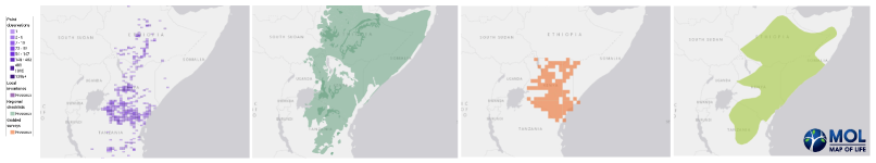
Figure 1. Species distribution models describe the relationship between environmental conditions and (actual or potential) species presence. However, the link between the environment and species distribution data can be complex, particularly since distributional data comes in many different forms. Above are four different sources of distribution data for the Von Der Decken’s Hornbill (hor, [n.d.]): (from left to right) raw point observations, regional checklists, gridded ecological surveys, and data-driven expert range maps. All images are from Map of Life (Jetz et al., 2012).

1. Introduction

Data collection method	Example	Observation type
Community science observations	iNaturalist	Presence-only
Community science checklists	eBird	Presence-absence
Static sensors	Camera traps	Presence-absence
Sample collection	Insect trapping	Presence-absence
Expert field surveys	Line transects	Presence-absence
Historic records, natural history collections	Herbarium sheets	Presence-only

Table 1. Sources of species observation data. Each of these examples represents a method of collecting or accessing observations of different species. One important distinction is whether the observations are presence-only or presence-absence. Presence-only data consists of locations where a species has been sighted. Presence-absence data also includes locations where a species was checked for but not observed.

Ecological research helps us to understand ecosystems and how they respond to climate change, human activity, and conservation policies. Much of this work starts by deploying networks of sensors (often cameras or microphones) to monitor the organisms living in a fixed study area. Ecologists must then invest significant effort to filter, label, and analyze this data. This step is often a bottleneck for ecological research. For example, it can take years for scientists to process and interpret a single season of data from a network of camera traps. In another case, building real-time estimates of salmonid escapement requires teams of field ecologists working in shifts to watch streams of sonar data 24 hours a day. The challenge is even greater for taxa that are studied by trapping specimens, such as beetles and other insects. Entomologists can collect thousands of beetles in a few days, but it may require months or years for a suitable expert to exhaustively identify all of the specimens to the species level.

Machine learning methods can significantly accelerate the processing and analysis of large repositories of raw data (iNa, [n.d.]; Wil, [n.d.]; LIL, [n.d.]; Berger-Wolf et al., 2017; GBI, [n.d.]), which can increase the speed and geographic scope of ecological analysis. For instance, ongoing collaborations between machine learning researchers and ecologists have lead to tremendous progress in automating species identification from images in community science data (Van Horn et al., 2018; Aodha et al., 2019) and camera trap data (Beery and Morris, 2019; Wil, [n.d.]). However, unfamiliar ecological concepts and terminology can present a barrier to entry for many computer scientists who might otherwise be interested in contributing to ecological problems. This is particularly true for more involved ecological problems which may not fit neatly into existing machine learning paradigms.

One such area is species distribution modeling (SDM): using species observations and environmental data to estimate the geographic range of a species. This problem has received significant attention from ecologists and statisticians, and there has been increasing interest in machine learning methods due to the large amounts of available data and the highly complex relationships between species and their environments. This document is meant to serve as an easy entry point for computer scientists interested in SDM. In particular, we aim to highlight the exciting technical challenges posed by SDM while also emphasizing the needs of end-users to encourage ecologically meaningful progress. Our hope is that this document can serve as a quick resource for computer science researchers interested in getting started working on conservation and sustainability applications.

The rest of this work is organized as follows. In Section 2 we discuss different ways to represent the distribution of a species. We discuss species distribution modeling in Section 3 and we consider other related ecological modeling problems in Section 4. In Section 5 we point out pitfalls and challenges in SDM. Finally, we provide pointers to available data (Section 6) and discuss open problems (Section 7).

2. Representing the distribution of species

The distribution of a species is typically represented as a map which indicates the spatial extent of the species. These maps can be created in a variety of ways, ranging from highly labor-intensive expert range maps to fully automatic species distribution models. We show four examples in Fig. 1. In this section we give a high-level overview of three important sources of maps: raw species observation data, predictions from statistical models, and expert knowledge.

2.1. Raw species observation data.

Any representation of the distribution of a species begins with some sort of species observation data. In general, species observation data consists of records indicating whether a species is present or absent at certain locations. Species observation data can take many forms – see Table 1 for examples. Species observation data falls into two general categories: presence-only data reports known sightings, or occurrences, of a species, while presence-absence data also provides information on where a species did not occur. Data collection strategies define whether absence data will be available. For instance, iNaturalist collects opportunistic imagery of species from community scientists, which produces presence-only species observations. On the other hand, eBird uses species checklists where all bird species seen and/or heard within a time span at a given location are reported. Since exhaustive reporting is expected from observers, any bird species not reported is assumed to be absent. In this sense, checklists are treated as presence-absence data.

One of the simplest ways to convey the distribution of a species is to simply show all of the locations where the species is known to be present or absent on a map. However, this sort of highly simplified “species distribution” is not able to make any predictions about whether a species might be present or absent at locations which have not been sampled.

2.2. Statistical models.

To create species distributions that can extrapolate beyond sampled locations, we can pair species observations with collections of environmental characteristics (altitude, land cover, humidity, temperature, etc.) and fit statistical models that use the environmental characteristics to predict species presence or absence. These models can make predictions at any place and time for which these environmental characteristics are known. Species distribution models fall into this category, and are our focus throughout this document.

2.3. Expert range maps.

Species range maps have traditionally been heavily influenced by the individual scientists who study those species. These maps are often based on a complex combination of heterogeneous information sources, including personal observations, understanding of the species’ habitat preferences, local knowledge/reports, etc. From our discussions with practitioners, we find that these expert range maps (ERMs) are often the most trusted source of distribution information. Perhaps the most widely-known expert range maps are those published by IUCN (Group et al., 2018) as part of their Red List of vulnerable and endangered species. An example of the IUCN range map for the caracal can be seen in Fig. 2. Studies have shown both agreement (Alhajeri and Fourcade, 2019) and disagreement (Hurlbert and White, 2005; Graham and Hijmans, 2006) between ERMs and species observation data. Expert range maps have also been found to be highly scale-dependent, tending to overestimate the occupancy area of individual species and ranges ¡ 200km (Hurlbert and Jetz, 2007). It is important to note that ERMs come in many forms, from hand-drawn maps to data-driven maps that are slightly refined by experts. In the latter case, ERMs are partially based on species observation data, so the two cannot be treated as independent sources. As we will discuss in more detail in Section 3.5, the lack of a solid “ground truth” information about the true underlying distribution of species across space and time makes it difficult to analyze the accuracy of any species distribution model, including those drawn by experts.

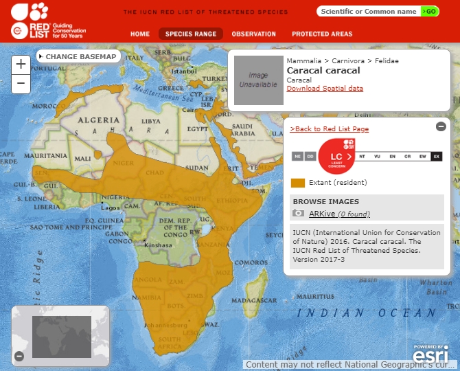
Figure 2. The International Union for Conservation of Nature (IUCN) publishes expert range maps for many species, particularly those on their “Red List of Threatened Species” (Vié et al., 2009). Here we show the IUCN Range Map for the Caracal caracal (Bahaa-El-Din et al., 2015).

3. Species Distribution Models

The terminology in this area can be confusing, so we will start with a definition and a few clarifications.

Intuitive definition. A species distribution model is a function that uses the characteristics of a location to predict whether or not a species is present at that location. This can be understood as a supervised learning problem. The input is a vector of environmental characteristics for a location and the output is species presence or absence. In principle one could use almost any classification or regression technique as the basis for an SDM.

Formal definition. The key components of a simple species distribution modeling pipeline are: (1) species observation data, (2) a method for encoding locations, and (3) a function which maps location encodings to predictions. Formally, we define these components as follows:

1. A dataset of species observations. This is a collection of records indicating that a species is present or absent at given location and time. We write this as $\{(\mathbf{x}_{i},y_{i})\}_{i=1}^{N}$ where $\mathbf{x}_{i}\in\mathcal{X}$ is a spatiotemporal location and $y_{i}\in\{0,1\}$ indicates presence ($1$) or absence ($0$). The spatiotemporal domain $\mathcal{X}$ is typically something like $\mathcal{X}=[0,180)\times[0,360)\times[0,1)$ which encodes global longitude and latitude as well as the time of year.

2. A location representation $h:\mathcal{X}\to\mathcal{Z}\subset\mathbb{R}^{k}$. This is typically a simple “look-up” operation, where $\mathbf{x}\in\mathcal{X}$ is cross-referenced with $k$ pre-defined geospatial data layers to produce a vector of location features $h(\mathbf{x})\in\mathbb{R}^{k}$. That is, $h(\mathbf{x})$ is a representation of the location $\mathbf{x}\in\mathcal{X}$ in some environmental feature space.

3. A model $f_{\theta}:\mathcal{Z}\to[0,1]$ where $\theta$ is a parameter vector. The goal is to find parameters $\theta$ of $f$ so that $f_{\theta}(h(\mathbf{x}))=1$ when the species is present and $f_{\theta}(h(\mathbf{x}))=0$ otherwise. This is usually framed as a supervised learning problem on the dataset $\{(h(\mathbf{x}_{i}),y_{i})\}_{i=1}^{N}$.

Note that this is a streamlined formalization meant to capture the essence of SDM. While there are many variants in practice, almost any species distribution modeling will include these core concepts.

What does an SDM actually predict? An SDM takes as input a vector of environmental features and predicts a numerical score (usually between $0$ and $1$) for a location. An important distinction to note regarding SDMs is geographic space vs. environmental space, elucidated in Fig. 3. This score is often interpreted as a prediction of habitat suitability. Typically the score may not be interpreted as the probability a species is present. Note that here we are only considering presence vs. absence - predicting species abundance is a more challenging problem, which we discuss in Section 4.2.

How is an SDM used? The most common end product is a map of the SDM predictions, which is produced by simply visualizing the SDM predictions across an area of interest. Binary predictions can be obtained by applying a threshold to the continuous predictions of the SDM.

3.1. A brief history of species distribution modeling

Early predecessors for SDM include qualitative works that link patterns within taxonomic groups to environmental or geographic factors, such as Joseph Grinnel’s 1904 study of the distribution of the chestnut-backed chickadee (Grinnell, 1904), among others (Murray, 1866; Schimper, 1903; Whittaker, 1956; MacArthur, 1958).

Modern SDMs are primarily statistical models fit to observed data. Early quantitative approaches used multiple linear regression and linear discriminant function analyses to associate species and habitat (Capen, 1981; Stuffer, 2002). The application of generalized linear models (GLMs) (Nelder and Wedderburn, 1972; Austin, 1985) provided more flexibility by allowing non-normal error distributions, additive terms, and nonlinear relationships. The explosive proliferation of large “presence-only” datasets (see Table 1) in recent years has led to the development of new modeling approaches to SDMs such as the popular “Maximum Entropy Modeling” (MaxEnt) approach (Phillips et al., 2006) with roots in point process modeling (Renner and Warton, 2013).

The first modern SDM computing package, BIOCLIM, was introduced in 1984 on the CSIRO network (Busby, 1991; Booth et al., 2014). This package took observation information, such as the species observed, location, elevation, and time, and used them to determine what environmental variables correlated with that species’ occurrence. These variables were then used to map possible distributions of the species under consideration. Climate interpolation techniques developed for BIOCLIM are the basis of the existing WorldClim database (Fick and Hijmans, 2017) and are still widely used in SDMs today. Many different implementations of various SDM methods are now publicly available. We would like to highlight Wallace (Kass et al., 2018), which is a well-documented R implementation of historic and modern techniques.

As earth observation technology has improved, the scope of what is possible to include as an environmental covariate in a model has vastly increased. Improvements in weather monitoring systems gave access to high-temporal-frequency temperature, wind, and precipitation measurements. Recently, ecologists have turned to remote sensing imagery to estimate high-spatial-coverage ecological variables such as soil composition or density of sequestered carbon, as well as mapping land cover type across regions (He et al., 2015). Modern SDM methods pair these covariate estimates with increasingly accurate global elevation maps, and selected high-quality but sparse in-situ measurements (Pradervand et al., 2014; Lassueur et al., 2006).

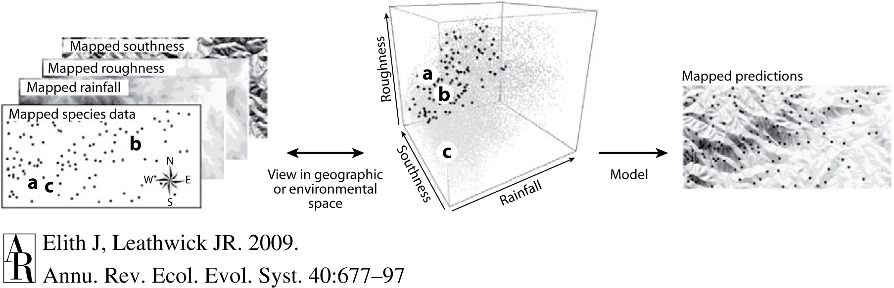
Figure 3. Geographic vs. environmental space. Observation data can be associated with a geographical location, or mapped into a feature space based on environmental covariates. Most SDMs operate under the assumption that with the right set of environmental variables and an appropriate model, one could use environmental characteristics to map species distribution. Figure reproduced with permission, originally published in (Elith and Leathwick, 2009).

Several excellent, detailed reviews of SDMs have been published within the ecology community (Elith and Leathwick, 2009; Guisan and Zimmermann, 2000; Stuffer, 2002; Guisan and Thuiller, 2005a; Richards et al., 2007; Schroeder, 2008). We direct the reader to the excellent summary by Elith and Leathwick (Elith and Leathwick, 2009).

3.2. Covariates for species distribution modeling

In this section we discuss several environmental characteristics (often called covariates) that can be used for species distribution modeling. Here we are focused on describing the different categories of covariates – details on specific covariate datasets are available in Section 6. Some of the covariates we discuss are widely used in the species distribution modeling literature, while others are more recent or speculative. It is also important to keep in mind that many covariates are themselves based on sophisticated predictive models due to the cost of densely sampling any property of the earth’s surface.

3.2.1. Climatic variables.

Temperature and precipitation are critical characteristics of an ecosystem. Perhaps the most commonly used climate dataset for SDM is the WorldClim bioclimatic variables (Fick and Hijmans, 2017) dataset, which provides 19 climate-related variables averaged over the period from 1970 to 2000 at a spatial resolution of around 1km². We show a few examples of variables from this dataset in the top row of Fig. 5.

3.2.2. Pedologic (soil) variables.

Soil characteristics are intimately related to the plant life in an area, which naturally influences the entire ecosystem. One example of a comprehensive pedologic dataset is SoilGrids250m (Hengl et al., 2017), which consists of soil properties like pH, density, and organic carbon content at a 250m² resolution globally. We show a few examples of variables from this dataset in the bottom row of Fig. 5.

3.2.3. Vegetation indices.

A vegetation index (VI) is a number used to measure something about the plant life in an area, and is typically computed from remote sensing data like satellite imagery. Many different VIs have been proposed. A review paper published in 1995 discussed 40 different vegetation indices that had been developed by different researchers (Bannari et al., 1995). One of the most popular examples is the normalized difference vegetation index (NDVI). If a remote sensing image includes the red and near-infrared (NIR) bands, then the corresponding NDVI image can be computed by applying the formula

(1) $$\mathrm{NDVI} =\frac{\mathrm{NIR}-\mathrm{Red}}{\mathrm{NIR}+\mathrm{Red}}$$

independently at each pixel. NDVI is meant to indicate the presence of live green plants. From a computer vision perspective, these VIs are essentially hand-designed features for remote sensing data.

3.2.4. Land use / land cover.

The term land cover refers to the physical terrain at a location, while the closely related term land use tends to emphasize the function of a location. For instance, an area with the land cover label “dense urban” may have a land use label like “school” or “hospital.” We provide an example in Fig. 4, which shows RGB imagery and land cover from two different sources for the same 1km² area. It is not obvious what the best label set would be for species prediction, but practically speaking many of the available land use / land cover datasets are focused on relatively coarse categories related to agriculture, natural resources, or urban development. For instance, the U.S. National Land Cover Database assigns one of 20 land cover classes to every 30m² patch of land in the United States at a temporal resolution of 2-3 years (Homer et al., 2015). The classes cover various general habitat types (water, snow, developed land, forests…) but are not tuned for species prediction in particular.

3.2.5. Measures of human influence.

Humans have had a profound impact on the natural world, so it is reasonable to include measures of human influence as environmental characteristics. For instance, the Human Influence Index (Sanderson et al., 2002) uses eight factors (human population density, railroads, roads, navigable rivers, coastlines, nighttime lights, urban footprint, and land cover) to compute a score that is meant to quantify how much an environment has been reshaped by humans.

3.2.6. Remote sensing imagery.

Imagery collected by satellites, planes, or drones can provide substantial information about an environment. To start with, we note that vegetation indices, land cover, land use, and many measures of human influence are all derived from some form of overhead imagery like that in Fig. 4. In addition, there may be more abstract patterns that can be extracted using modern computer vision techniques like convolutional neural networks. Research on the use of raw overhead imagery (instead of derived products) for SDM is in its early stages (Tang et al., 2018; Cole et al., 2020; Dobrowski et al., 2008).

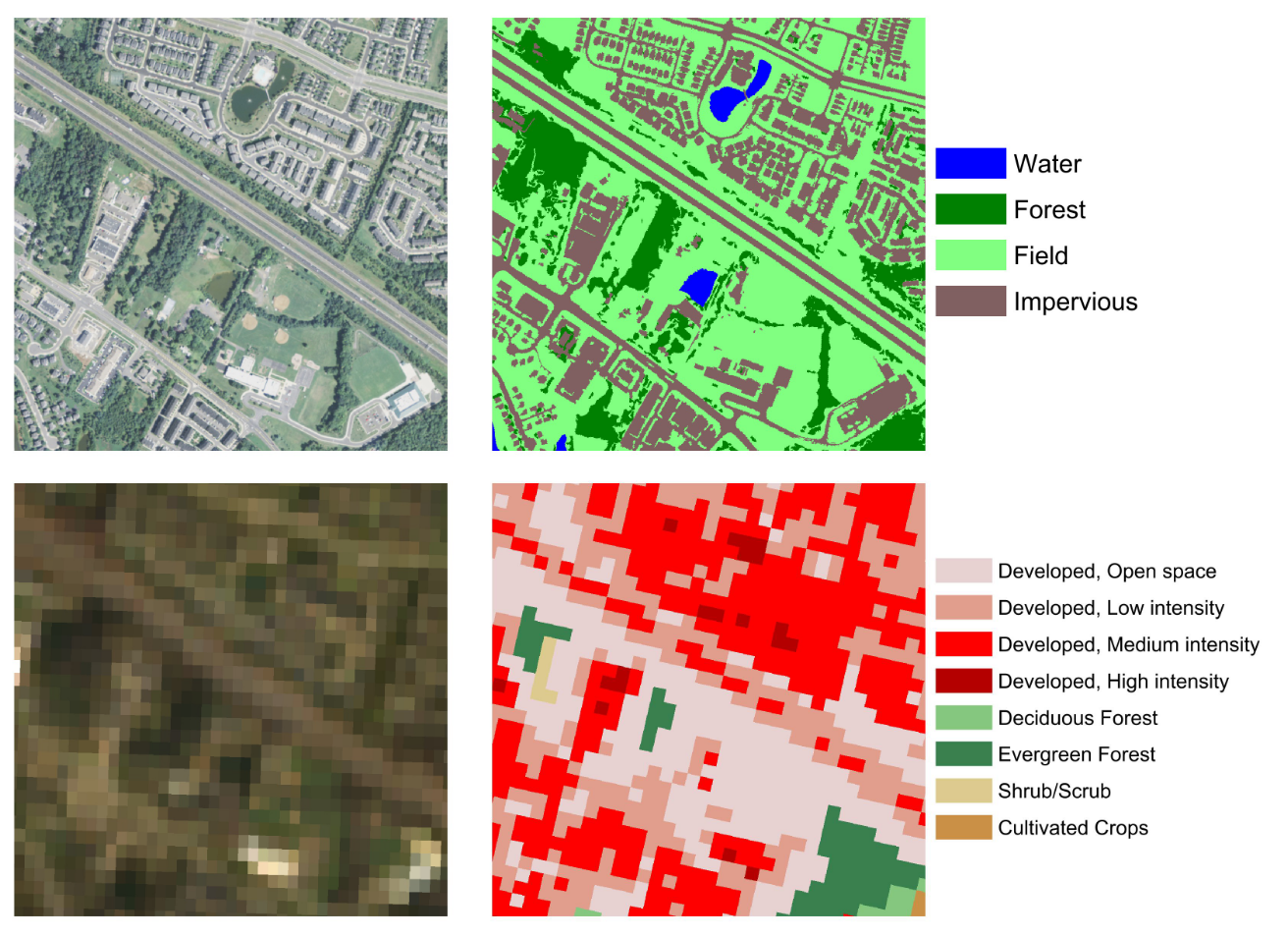
Figure 4. RGB imagery (left column) and land cover maps (right column) from two different remote sensing sources covering the same 1km² area, from (Robinson et al., 2019). RGB imagery is manually or semi-automatically annotated to produce the land cover labels. As this example demonstrates, the set of land cover labels can vary depending on the organization doing the labeling. Figure reproduced with permission, originally published in (Robinson et al., 2019).

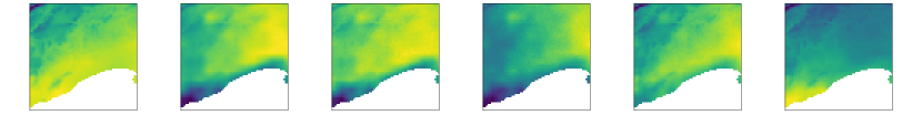
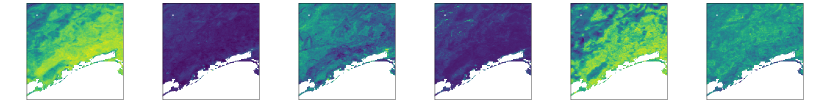
Figure 5. Visualizations of some of the bioclimatic variables (top row: bio_1 - bio_6 from left to right) and pedologic variables (bottom row: orcdrc, phihox, cecsol, bdticm, clyppt, sltppt from left to right) provided for the GeoLifeCLEF 2020 competition (Cole et al., 2020). The area shown in each image is approximately 64 km² centered in Montpellier, France. While we visualize each environmental variable as a 2D raster, most species distribution modeling methods are only compatible with relatively low-dimensional vectors of environmental variables (not “stacks” of 2D patches). As is typical in a collection of covariates, we see that the pedologic variables have a different resolution than the bioclimatic variables.

3.3. Properties of species distribution models

In this section we describe important properties that can be used to categorize species distribution models. Any particular species distribution model may or may not have any of these properties. The categories we describe are in general nested or overlapping, not mutually exclusive.

3.3.1. Presence only vs. presence-absence models.

Species observation datasets may be either presence-absence or presence-only. While presence-only data is easier to collect, the are limitations on what can be estimated from such data (Hastie and Fithian, 2013). Typically a species distribution model is designed to handle either presence-absence or presence-only data, though there is growing interest in developing methods that can use both (Gormley et al., 2011; Pacifici et al., 2017a; Fletcher Jr et al., 2019).

3.3.2. Single vs. multi-species models.

Many SDMs are designed to model the distribution of a single species. This is in contrast to multi-species models which are meant to capture information about several species. Many of the earlier models are single-species models (Phillips et al., 2006; Elith and Leathwick, 2009), though interest in multi-species models has grown over time (Hui et al., 2013; Harris, 2015; Norberg et al., 2019a).

3.3.3. Multi-species models: stacked vs. joint

Multi-species SDMs can be classified as either stacked or joint. In a stacked model, a single-species SDM is fit for each species and the resulting maps are “stacked” on top of one another to provide a multi-species map. This approach is simple, but it cannot take advantage of patterns in how species co-occur. This is the motivation for joint SDMs, in which the estimated distribution of each species also depends on occurrence data for other species. Recent work has begun to systematically compare the results from stacked and joint species distribution models for different species and regions (Henderson et al., 2014; Norberg et al., 2019a; Zurell et al., 2020).

3.3.4. Spatially explicit models.

Typically species distribution models use environmental characteristics to make predictions about the presence or absence of species. Such models represent a location in terms of these environmental features, so two different locations with the same environmental characteristics will lead to the same predictions, even though the two locations may be far apart. Models that mitigate this concern by incorporating geographical location information directly are referred to as spatially explicit (Domisch et al., 2019) models.

3.3.5. Occupancy models.

It is easier to confirm that a species is present than it is to confirm that a species is absent. One confident observation of a species suffices to confirm its presence at a given location. However, failing to observe a species at a location does not suffice to prove absence, since the species could have been present but not observed. Occupancy models are meant to account for imperfect detection by modeling the probability that a species is present but unobserved at a given location conditional on the sampling effort that has been invested (MacKenzie et al., 2002; Bailey et al., 2014).

3.3.6. Understanding uncertainty and error.

Species distribution models attempt to capture the behavior of a complex system from data, which is a challenging and error-prone process. (Rocchini et al., 2011) describes 11 sources of uncertainty and error in species distribution models, and groups them into two clusters: (i) uncertainty in the observation data itself and (ii) uncertainty due to arbitrary modeling choices. (Dormann et al., 2008) studies the effect of making different reasonable modeling choices on final projections of species distribution under different future climate scenarios. Similarly, (Synes and Osborne, 2011) considers the uncertainty introduced by the arbitrary choice of covariates while (Stoklosa et al., 2015) analyzes the effect of uncertainty in the values of the covariates themselves. (Naimi et al., 2014) focuses on the effect of uncertainty in the location of species observations. (Beale and Lennon, 2012) reviews sources of uncertainty for different types of species distribution models, as well as best practices for minimizing uncertainty and methods for incorporating uncertainty directly into the model.

3.4. Algorithms for species distribution modeling

In this section we provide a high-level overview of the space of algorithms commonly used for species distribution modeling in the ecological community. This section draws heavily from the organization of (Norberg et al., 2019a), which is an excellent comparative study of different species distribution modeling techniques. We discuss several commonly used models, and note that the different methods can have very different properties, assumptions, and use cases. Unlike some classes of algorithms, different species distribution modeling methods are generally not readily interchangeable.

3.4.1. Presence-only methods.

Perhaps the most popular approach for presence-only SDM is MaxEnt (Phillips et al., 2006). We follow the description given in (Elith et al., 2011). The basic idea is to estimate the probability of observing a given species as a function of the environmental covariates. The estimate is chosen to be (i) consistent with the available species observation data and (ii) as close as possible (in KL divergence) to the marginal distribution of the covariates. Criterion (ii) is necessary because there are typically many distributions that satisfy criterion (i). Another simple approach for presence-only SDM is to introduce artificial negative observations called pseudonegatives or pseudoabsences based on some combination of domain knowledge and data. Once pseudonegatives have been generated, they are combined with the presence-only data and traditional presence/absence methods are applied.

3.4.2. Traditional statistical methods.

Perhaps the most common methods in species distribution modeling are workhorse methods drawn from the statistics literature such as generalized linear models (Friedman et al., 2010; Foster and Dunstan, 2010; Wang et al., 2012; Venables and Ripley, 2013; Ovaskainen et al., 2017). Important special cases include logistic regression (Pearce and Ferrier, 2000) and generalized additive models (Wood, 2011). Some species distribution modeling algorithms are better thought of as general frameworks whose particular realization depends on the available data sources and modeling goals. As an example, the Hierarchical Modeling of Species Communities (HMSC) framework (Ovaskainen et al., 2017) minimally requires species occurrence data with corresponding environmental features. The species occurrences are related to environmental features by a generalized linear model. However, the framework can be extended to incorporate e.g. information on species traits and evolutionary history.

3.4.3. Machine learning methods.

The relationship between species and their environment is complex and may not satisfy traditional statistical assumptions such as linear dependence on covariates or i.i.d. sampling. For this reason, machine learning approaches have also enjoyed considerable popularity in the species distribution modeling literature. Examples include boosted regression trees (Elith et al., 2008), random forests (Cutler et al., 2007), and support vector machines (Drake et al., 2006). In addition, neural networks have been used for species distribution modeling since well before the deep learning era (Broomhead and Lowe, 1988; Özesmi and Özesmi, 1999; Yen et al., 2004; Tirelli and Pessani, 2009). Interest in joint species distribution modeling with neural networks has only grown as deep learning has come to maturity (Harris, 2015). Convolutional neural networks in particular have created a new opportunity: the ability to extract features from spatial arrays of environmental features (Chen et al., 2016; Deneu et al., 2019) instead of using hand-selected environmental feature vectors.

3.5. The challenge of evaluation

How can we tell whether a species distribution model is performing well or not? The typical approach in machine learning is to use the model to make predictions on a held-out set of data and compute an appropriate performance metric by comparing the model predictions to ground-truth labels. But what is “ground truth” for a species distribution model?

3.5.1. Notions of Ground Truth

We describe several common approaches to the challenging problem of how to evaluate SDMs in practice. For further detail, (Mouton et al., 2010) provides an excellent discussion of different metrics for evaluating SDMs and the extent to which they are ecologically meaningful.

Compare against presence-absence data. Ideally, for each location, an expert observer would determine whether each species of interest is present or absent at that location. Conducting this kind of survey for a single species in a limited area is expensive, and the survey would need to be repeated periodically to monitor change over time. These exhaustive surveys quickly become extraordinarily expensive as we expand the number of species of interest or the geographic extent of the survey. Even if the resources were available, the observations would have some degree of noise - in particular, confirming that a species is absent from an area can typically only be done up to some degree of certainty. (See the discussion of occupancy modeling in Section 3.3.5.) For most species and most locations on earth, this sort of ideal ground truth data is just not available. However, this kind of evaluation is possible for select species and locations at sparse time points. For instance, (Elith et al., 2020) includes presence-absence data for 226 species from 6 parts of the world collected at various time points.

Compare against presence-only data. Unfortunately, presence-absence data is often unavailable. We describe a few simple methods for comparing predictions against presence-only data along with their shortcomings.

• False negative rate: how often are locations which are known to be positive predicted to be negative? The false negative rate measures whether the model is consistent with the observed positives, but does not assess the model’s behavior at other points.

• Top-$k$ classification accuracy: how often is the observed species among the $k$ most likely species under the model? However, there is not an obvious way to choose $k$. Moreover, for any fixed $k$ it is likely that some locations will have more than $k$ species while others will have fewer.

• Adaptive top-$k$ classification accuracy: this is a variant of the top-$k$ classification accuracy that assumes that the number of species is $k$ on average, while allowing some locations to have more than $k$ species while others may have fewer. See (Cole et al., 2020) for details. Like standard top-$k$ classification accuracy, choosing $k$ may be difficult.

Note that adaptive top-$k$ and top-$k$ are both metrics for multi-species models, while the false negative rate can be computed for single species models as well.

Compare against community science data. Community science projects like iNaturalist and eBird are generating species observation data at an extraordinary rate and frequency. iNaturalist alone generates millions of species observations per month (ina, [n.d.]). However, the data produced by such projects can vary in terms of how easy it is to use and interpret depending on the sampling protocol (Kosmala et al., 2016). For instance, iNaturalist accepts presence-only observations, which allows the user base to scale broadly but limits the utility of the data for ground truthing. iNaturalist data tells us where different species have been observed by humans, but not where those species are either absent or present without human observation. eBird uses a more rigorous sampling protocol that records both presences and absences, but their observations are limited to birds. The quality of these reports depends on the skill of the user at identifying all bird species they see or hear. Citizen science data has been found to produce results similar to those from (coarse) professional surveys under the right circumstances (Higa et al., 2014; Tye et al., 2016; Kosmala et al., 2016).

Compare against expert range maps. Another possibility is to compare the model predictions against one or more range maps that are hand-drawn by experts (see Section 2). However, this raises the question: how do we validate those range maps? A hand-drawn map may be biased by an individual’s experience or by the data sources the expert prefers. In addition, it can be difficult to find a suitable expert to generate a map for every species of interest. Another challenging question relates to temporal progression: is each expert updating their maps according to the latest data? If so, when was that data collected? The IUCN has a published set of standards for creating species range maps (Group et al., 2018), but not all creators of maps match these standards.

In addition, there is the methodological question of how one should evaluate a model against an expert range map, which is explored in (Mainali et al., 2020). Approaches range from very qualitative (ask an expert whether the map looks reasonable to them) to very quantitative (compute a well-defined error metric between the SDM predictions and the expert range map). Important to note here, expert range maps are most often categorical, with hard boundaries drawn representing temporal categories like “breeding”, “non-breeding”, “year-round”, etc. On the other hand, SDM predictions are often real-valued on $[0,1]$ over both space and time. While continuous predictions can be converted to binary maps by applying a threshold, it can be unclear how to choose this threshold if a robust validation method is not available.

Evaluation on downstream tasks. Instead of evaluating whether a species distribution model produces a faithful map of species presence, we may instead check whether it is useful for some other downstream task. For example, (Aodha et al., 2019) builds a simple SDM and demonstrates that it improves accuracy on an image-based species classification task. However, it is certainly possible for an SDM to be useful whether or not it accurately reflects the true species distribution.

3.5.2. Evaluation pitfalls

Even when suitable ground truth data is available, there are some pitfalls that can hinder meaningful evaluation. In this section we discuss some of these pitfalls and make specific recommendations to the machine learning community for handling them.

Performance overestimation due to spatial autocorrelation. In the machine learning community it is common to sample a test set uniformly at random from the available data. However, this strategy can lead to overestimation of algorithm performance for spatial prediction tasks since it is possible to obtain high performance on a uniformly sampled test set by simple interpolation (Roberts et al., [n.d.]). This effect is called spatial autocorrelation. Similar concerns are relevant for evaluating camera trap image classifiers (Beery et al., 2018). For ecological tasks, it is important to evaluate models as they are intended to be used. In many cases, the more ecologically meaningful question is whether the model generalizes to novel locations, unseen in the training set. In these cases it is important to create a test set by holding out spatial areas. In other cases, the ecologist seeks to build a model that will perform accurately in the future at their set of monitoring sites. In these cases, instead of holding out data in space, we can split the data to hold out a test set based on time. A randomly sampled test set is not a good proxy for the use case of either scenario.

Hyperparameter selection. The performance of an algorithm typically depends on several hyperparameters. In the machine learning community these are set using cross-validation on held-out data. However, selecting and obtaining a useful validation set can be particularly challenging in SDM due to the data collection challenges described elsewhere. Recent work has also studied the sensitivity of SDMs to hyperparameters (Hallgren et al., 2019) and developed techniques for hyperparameter selection in the presence of spatial autocorrelation (Schratz et al., 2019).

Spatial quantization. A natural first step when working with spatially distributed species observations is to define a spatial quantization scheme. By “binning” observations in this way, we can associate many species observations with a single vector of covariates. Additionally, spatially quantized data can be more natural from the perspective of many machine learning algorithms since the domain becomes discrete. However, the choice of quantization scheme (grid cell size) is difficult to motivate in a rigorous way. This is a problem because different quantization choices can result in vastly different outcomes - this is known as the modifiable areal unit problem (Openshaw, 1984). It is possible to cross-validate the quantization parameters, but only in those limited cases where there is enough high-quality data for this to be a reliable procedure. Furthermore, that process may be computationally expensive.

The long tail. Many real-world datasets exhibit a long tail: a few classes represent a large proportion of the observations, while many classes have very few observations (Van Horn and Perona, 2017; Beery et al., 2018). Species observation data is no exception - for example, in the Snapshot Serengeti camera trap dataset (Swanson et al., 2015) there are fewer than 10 images of gorillas out out of millions of images collected over 11 years. This presents at least two problems. The first problem is that standard training procedures will typically result in a model that perform well on the common classes and poorly on the rare classes. The second is that many evaluation metrics are averaged over all examples in the dataset, which means that the metric can be very high despite poor performance on almost all species. It is much more informative to study the performance on each class or on groups of classes (e.g. common classes vs. rare classes). One common solution is to compute metrics separately for each class and then average over all classes to help avoid bias towards common classes in evaluation.

3.5.3. Model trust

Once a model has been built, the previously discussed challenges of model evaluation make it difficult to determine where, how much, and for how long a model is sufficiently accurate to be used. The accuracy needed may also vary by use case and subject species. In our discussions with ecologists, we find that this leads to a lack of trust in SDMs. What verification and quality control is needed to ensure a model is still valid over time? This is an open question, and an important one to answer if our models are to be used in the real world.

4. Other types of ecological models

Species distribution modeling is only one of many ways that ecologists seek to describe and understand the natural world. To give readers a sense of how SDM fits into the broader scope of ecological modeling, we provide a high-level overview of other common modeling tasks.

4.1. Mechanistic models

Mechanistic models make assumptions about how species depend on the environment or on other species. One example is to use an understanding of a plant’s biology to predict the viable temperature range where the plant can grow (Sweeney and Hopkinson, 1975). Such models are useful but difficult to scale, as they require species-specific expert knowledge. Our focus in this work is on correlative species distribution models, which do not require mechanistic knowledge.

4.2. Abundance modeling

Abundance modeling goes beyond species presence or absence, aiming to characterize the absolute or relative number of individuals at a given location. We define abundance and related concepts in Section 4.3.

4.2.1. Population estimation

Population estimation is concerned with counting the total number of individuals of a species, typically within some defined area (Schnabel, 1938). Population size is most frequently estimated using capture-recapture models, which require the ability to distinguish between individuals of the same species. Traditionally this individual re-identification was based on physical tags or collars (Grimm et al., 2014), but some recent efforts have relied on the less invasive method of identifying visually distinctive features, such as stripe patterns or the contour of an ear (Berger-Wolf et al., 2017).

4.2.2. Density estimation

Density estimation seeks to model spatial abundance, the abundance of a species per unit area, to understand where a species is densely versus sparsely populated (Rowcliffe et al., 2008; Verberk, 2011).

4.2.3. Data collection procedures for abundance

As mentioned above, capture-recapture requires an individual to be re-identifiable. In the absence of the ability to re-identify individuals, several other data collection procedures are used. One that is frequently used for insects and fish populations is the harvest method, where individuals are collected in traps which are open for a set amount of time and then counted (Pope et al., 2010; Seibold et al., 2019). Sampling strategies for other taxa include:

• Quadrat sampling. A quadrat is a fixed-size area where species are to be sampled. Within the quadrat, the observer exhaustively determines the occurrence and relative abundance of the species of interest. Quadrat sampling is most commonly used for stationary species like plants. The observer will sample quadrats throughout the region of interest to derive sample variance and conduct further statistical analysis (Hanley, 1978).

• Line intercept sampling. A line intercept or line transect is a straight line that is marked along the ground or the tree canopy, and is primarily used for stationary species (Heady and Gibbens, 1959). The observer proceeds along the line and records all of the specimens intercepted by the line. Each transect is regarded as one sample unit, similar to a single quadrat.

• Cue counting. Cue counting is based on observing cues or signals that a species is nearby, such as whale or bird calls. It is used primarily for species that are underwater or similarly difficult to sight (Marques et al., 2011).

• Distance sampling. Distance sampling refers to a class of methods which estimate the density of a population using measured distances to individuals in the population (Buckland et al., 2005). Distance sampling can be added to line transects in order to incorporate specimens that are off the transect line but still visible. Appropriately calibrated camera traps can also benefit from distance sampling (Rowcliffe et al., 2008).

• Environmental DNA (eDNA) sampling. Samples of water or excrement collected in the field can be sequenced to provide species identifications. The ratios of environmental DNA for each species can be used to estimate abundance (Lodge et al., 2012; Valentini et al., 2016).

Each of these procedures produces different types of data, and each method comes with its own innate collection biases. These biases can add to the challenge of evaluating ecological models, as discussed in Section 3.5.

4.3. Biodiversity measurement and prediction

While it is important to understand the distribution of particular species, in many cases the ultimate goal is to understand the health of an ecosystem at a higher level. Biodiversity is a common surrogate for ecosystem health, and there are many different ways to measure it (Whittaker, 1960; Jost, 2006, 2007). In this section we define and discuss several biodiversity metrics and related concepts. Note that some sources give different definitions than those presented here, so caution is warranted.

We now define some preliminary notation. We let $R$ denote an arbitrary spatial unit such as a country. Many biodiversity metrics are computed based on a partition of $R$ into $N$ sub-units, which we denote by $\{R_{i}\}_{i=1}^{N}$. The choice of partition can have a significant impact on the value of some metrics, but for the purposes of this section we simply assume a partition has been provided.

Species richness. The species richness of $R$ is the number of unique species in $R$, which we write as $S(R)$.

Absolute abundance. The absolute abundance of species $k$ in $R$ is the number of individuals in $R$ who belong to species $k$. We write this as $A_{k}(R)$.

Relative abundance. The relative abundance of species $k$ in $R$ is the fraction of individuals in $R$ who belong to species $k$, which is

(2) $$p_{k}(R)=\frac{A_{k}(R)}{\sum_{j=1}^{S(R)}A_{j}(R)}.$$

Since $\sum_{j=1}^{S(R)}p_{j}(R)=1$ and $p_{j}(R)\geq 0$ for all $j\in\{1,\ldots,S(R)\}$, the vector of relative abundances $\mathbf{p}(R)=(p_{1}(R),\ldots,p_{S(R)}(R))$ forms a discrete probability distribution. The species richness can then be alternately defined as the support of this distribution, given by

(3) $$S(R)=|\{j\in\{1,\ldots,S(R)\}:p_{j}(R)>0\}|.$$

Of course we can replace $p_{j}$ with $A_{j}$ everywhere and get an identical quantity.

Shannon index. The Shannon index of $R$ is the entropy of the probability distribution $\mathbf{p}(R)$, so

(4) $$H(\mathbf{p}(R))=-\sum_{j=1}^{S(R)}p_{j}(R)\log p_{j}(R).$$

The Shannon index quantifies the uncertainty involved in guessing the species of an individual chosen at random from $R$. Sometimes $H$ is instead written as $H^{\prime}$, and sometimes the argument is written as $R$ instead of $\mathbf{p}(R)$.

Simpson index. The Simpson index of $R$ is the probability that two individuals drawn at random from the dataset (with replacement) are the same species, and is given by

(5) $$\lambda(R)=\sum_{i=1}^{S(R)}p_{i}^{2}.$$

Alpha diversity. The alpha diversity of $R$ is the average species richness across the sub-units $\{R_{i}\}_{i=1}^{N}$, given by

(6) $$\alpha(R)=\frac{1}{N}\sum_{i=1}^{N}S(R_{i}).$$

Gamma diversity. The gamma diversity of $R$ is defined as

(7) $$\gamma(R,q) =\left(\sum_{j=1}^{S(R)}p_{j}^{q}\right)^{1/(1-q)}$$

where $q\in[0,1)\cup(1,\infty)$ is a weighting parameter (Jost, 2006). Note that gamma diversity is also commonly denoted by ${}^{\gamma}D_{q}(R)$. There are several interesting special cases:

• If $q=0$ then gamma diversity reduces to species richness i.e. $\gamma(R,0)=S(R)$.

• Gamma diversity is also related to the Shannon index, since $\lim_{q\to 1}\gamma(R,q)=\exp H(\mathbf{p}(R))$(Jost, 2006).

• If $q=2$ then gamma diversity reduces to the inverse of the Simpson index i.e. $\gamma(R,2)=1/\lambda(R)$.

Beta diversity. The beta diversity of $R$ is meant to measure the extent to which sub-units $R_{i}$ are ecologically differentiated. This can be interpreted as a measure of the variability of biodiversity across sub-regions or habitats within a larger area. It is defined as

(8) $$\beta(R,q)=\frac{\gamma(R,q)}{\alpha(R)}$$

where $q$ is the same weighting parameter we say in the definition of gamma diversity (Tuomisto, 2010; Jost, 2006). Beta diversity quantifies how many sub-units there would be if the total species diversity of the region $\gamma$ and the mean species diversity per sub-unit $\alpha$ remained the same, but the sub-units had no species in common.

5. Common challenges and risks

5.1. Differences in tools

R is the dominant coding language in ecology and statistics, but Python is dominant in machine learning. This language barrier limits code sharing, which in turn limits algorithm sharing. It is also important to note that some machine learning models are extremely computationally demanding to train, and some ecologists may not have access to the necessary computational resources.

5.2. Differences in ideas and terminology

Differences in concepts and terminology can make it difficult for machine learning practitioners to find and read relevant work from the ecology community (and vice-versa). However, there is a growing body of interdisciplinary work which brings ecologists and computer scientists together (AI_, [n.d.]a, [n.d.]b, [n.d.]c). It is important for computer scientists working in this area to establish ties with ecologists who can help them understand how to make ecologically meaningful progress.

5.3. Combining data sources

Species observation data is collected according to many different protocols, which means that effectively combining different data sources can be nontrivial (Pacifici et al., 2016; Koshkina et al., 2017; Miller et al., 2019; Gelfand and Shirota, 2019). For instance, observations collected in a well-designed scientific survey have significantly different collection biases from observations collected via iNaturalist. Handling these biases in a robust, systematic way can be quite challenging, particularly for large collections of data encompassing thousands of different projects, each with their own sampling strategies. In many cases, understanding the protocols used for a specific data collection project within a larger repository requires one to delve into the literature for that project. However, for many projects there do not exist accessible, standardized definitions or quantitative analysis of bias.

5.4. Black boxes, uncertainty, and interpretability

Machine learning models are frequently “black boxes,” meaning that it is difficult to understand how a prediction is being made. Ecologists are accustomed to models that are simpler to inspect and analyze, where they can confidently determine what factors are most important and what the effect of different factors might be. Because the results of ecological models are used to drive policy, being able to interpret how a model is making predictions and avoid inaccuracies due to overfitting is important. This is closely related to trust (or lack thereof) in model outputs and the need for uncertainty quantification, particularly in scenarios where models are being asked to generalize to new locations or forward in time.

5.5. Norms surrounding data sharing and open sourcing in ecology

Computer science has benefited from strong community norms promoting public data and open-sourced code. One consequence of this shift is that it is easy for computer scientists to take data for granted and to be frustrated when a scientist is unwilling to share their data publicly. However, it is important to remember that in some fields data can be extremely expensive to collect and curate. The cost of the hardware, travel to the study site, and the time needed to place the sensors and maintain the sensor network quickly adds up. Add to this the number of hours it takes for an expert to process and label the data so that it is ready for analysis, and it is easy to see why a researcher would want to publish several papers on their hard-won data before sharing it publicly. On the other hand, public datasets like those hosted on LILA.science (LIL, [n.d.]) have clear benefits for the community such as promoting reproducible research. Properly attributing data to the researchers who collected it (e.g. through the use of “DOIs for datasets” (Robertson et al., 2019)) could encourage more open data sharing in ecology. Data sharing norms are changing and many researchers are now happy to share their data and are pushing for more open data practices (Powers and Hampton, 2011; Reichman et al., 2011), but it is important to be aware of this cultural difference between computer science and other fields.

5.6. Model handoffs, deployment, and accessibility

Once a machine learning method has been rigorously evaluated and found to be helpful, it is important to ensure these techniques are accessible to those who can put them to good use. In computer science, we have a culture of ”open code, open data” which means that for most papers, all of the data and code is publicly available. However, ecologists may be less familiar with machine learning packages like PyTorch and TensorFlow, and may not have access to the computational resources required to train models on their data. If a method is to have real impact for the ecology community, it is important to provide models and code in a format that is accessible to end-users and well-documented. If the model is meant to become an integral part of an ecology workflow, plans for model maintenance and upkeep should be discussed.

5.7. Sensitive species

It is common for ecologists to obfuscate geolocation information before publishing any data containing rare or protected species to avoid poaching or stress from ecotourism. However, it is unclear whether obfuscation of GPS signal is sufficient to obscure the location of a photograph. It may be that a better solution is to remove any photos containing sensitive species, or to restrict sensitive access to a list of verified members of the research community. Second, the obfuscation distance of GPS location in published datasets might have a large effect on the accuracy of an SDM or other ecological model, particularly when both the training and validation data have been obfuscated. This obfuscation will further effect the reproducibility of a study, as results with or without obfuscation might be quite different.

6. What data is available and accessible?

There is an increasing number of publicly available ecological datasets that can be used for model training and evaluation. In this section we provide a few useful data sources as a starting point. We make a distinction between “analysis-ready” datasets which package species observations and covariates together and other data sources which can be combined to produce analysis-ready datasets.

6.1. Traditional analysis-ready datasets for multi-species distribution modeling

• The comprehensive SDM comparison in (Norberg et al., 2019a) uses five presence-absence datasets covering different species and parts of the world. Each dataset has a different set of covariates (min 6, max 38) and a different set of species (min 50, max 242). The datasets are available for download on Zenodo (Norberg, 2019).

• The recently released benchmark dataset (Elith et al., 2020) covers 226 species from 6 regions. Each region has a different set of covariates (min 11, max 13) and a different set of species (min 32, max 50).

Note that many “traditional” SDM datasets may not be large enough to train some of the more data-hungry machine learning methods.

6.2. Large-scale analysis-ready datasets for multi-species distribution modeling

• The GeoLifeCLEF datasets combine 2D patches of covariates with species observations from community science programs. The GeoLifeCLEF 2020 dataset (Cole et al., 2020) consists of 1.9M observations of 31k plant and animal species from France and the US, each of which is paired with high-resolution 2D covariates (satellite imagery, land cover, and altitude) in addition to traditional covariates. Previous editions of the GeoLifeCLEF dataset (Deneu et al., 2018; Botella et al., 2019) are also available, and are suitable for large-scale plant-focused species distribution modeling in France using traditional covariates. Note that all of the GeoLifeCLEF datasets are based on presence-only observations, so performance is typically evaluated using information retrieval metrics such as top-$k$ accuracy.

• The eBird Reference Dataset (ERD) (Munson et al., 2011) is built around checklists collected by eBird community members. In particular, it is limited to checklists for which the observer (i) asserts that they reported everything they saw and (ii) quantified their sampling effort. This allows unobserved species to be interpreted as absences if sufficient sampling effort has been expended. The resulting presence/absence data is combined with land cover and climate variables. Unfortunately, the ERD does not appear to be maintained or publicly available as of November 2020.

6.3. Sources for species observation data

• The Global Biodiversity Information Facility (GBIF) (GBI, [n.d.]) aggregates and organizes species observation data from over 1700 institutions around the world. We discuss a few specific contributors below.

• iNaturalist (iNa, [n.d.]) is a community science project that has produced over 70 million point observations of species across the entire taxonomic tree. The data can be noisy as it is collected and labeled by non-experts.

• eBird (eBi, [n.d.]) is a community science project hosted by the Cornell Lab of Ornithology which has produced more than 77 million birding checklists. These checklists provide both presence and absence, but absences can be noisy as it is possible the birder did not observe every species that was present at a given location.

• Movebank (Mov, [n.d.]) is a database of animal tracking data hosted by the Max Planck Institute of Animal Behavior. It contains GPS tracking data for individual animals, covering 900 taxa and including 2.2 billion unique location readings.

6.4. Sources for covariates

Earth observation datasets and their derived products can be freely obtained from many sources, including the NASA Open Data Portal (nas, [n.d.]), the USGS Land Processes Distributed Access Data Archive (lpd, [n.d.]), ESA Earth Online (esa, [n.d.]), and Google Earth Engine (ear, [n.d.]). Also see the detailed discussion of covariates in Section 3.2.

6.5. Sources for training species identification models

Species observation data can be produced by classifying the species found in geolocated images. Those who are interested in the species classification problem may be interested in the datasets below.

• The iNaturalist species classification datasets (Van Horn et al., 2018, 2021) are curated species classification datasets built from research-grade observations in iNaturalist.

• LILA.science (LIL, [n.d.]; Beery et al., 2018; Norouzzadeh et al., 2018) hosts a number of biology-focused image classification datasets, including camera trap datasets covering diverse species and locations.

• The Fine-Grained Visual Categorization (FGVC) workshop (FGV, [n.d.]) at CVPR hosts a number of competitions each year (FGV, [n.d.]; Beery et al., 2019b, a, 2020, 2021; Van Horn et al., 2018; Thapa et al., 2020; Tan et al., 2019; Mwebaze et al., 2019) which focus on species classification and related biodiversity tasks.

7. Open Problems

There are many open problems in SDM that may benefit from machine learning tools. In this section we discuss a few of these problems which we find particularly interesting.

7.1. Scaling up, geospatially and taxonomically

One of the main challenges in modern SDMs is scale. This includes scaling up SDMs to efficiently handle large geographic regions (Thuiller et al., 2008; Kissling et al., 2018; Jetz et al., 2019), many-species communities (Norberg et al., 2019b; Wilkinson et al., 2019; Pichler and Hartig, 2020; Tikhonov et al., 2020), and large volumes of training data (Merow et al., 2013; Wilkinson, 2019; Tikhonov et al., 2020). One particularly interesting question is whether jointly modeling many species could lead to SDMs which are significantly better than those based on modeling species independently.

7.2. Incorporating ecological theory and expert knowledge

There is a considerably amount of domain knowledge and ecological theory which would ideally be incorporated into SDMs (Guisan and Thuiller, 2005b). This might include knowledge about species dispersal  (Franklin, 2010; Barve et al., 2011; Miller and Holloway, 2015; Di Musciano et al., 2020), spatial patterns of community composition  (D’Amen et al., 2015; Chen et al., 2017; Joseph, 2020), and constraints on species ranges (e.g. cliffs, water)  (Fitzpatrick and Hargrove, 2009; Ewers et al., 2010; Miller and Holloway, 2015; Cooper and Soberón, 2018). Another area of significant interest is to factor in cross-species biological processes such as niche exclusion/competition  (Wiens, 2011; Poggiato et al., 2021), predator/prey dynamics (Trainor et al., 2014; Dormann et al., 2018; Poggiato et al., 2021), phylogenetic niche evolution (Pearman et al., 2008; Gavin et al., 2014; Chapman et al., 2017), or models linked across functional traits (Pollock et al., 2012; Clark et al., 2017; Vesk et al., 2021). These types of “domain-aware” algorithms are an active research area in the machine learning community (Bishop, 2013; Gu et al., 2016; Swischuk et al., 2019; Doll et al., 2012).

7.3. Fusing data

A third open area of investigation centers on how to best incorporate and utilize data collected at different spatiotemporal scales or in heterogeneous formats. This includes combining presence-only, presence-absence, abundance, and individual data such as GPS telemetry data (Johnson and Gillingham, 2008; Phillips and Elith, 2011; Pacifici et al., 2017b; Fieberg et al., 2018). It also includes multi-scale or cross-scale modeling (Václavík et al., 2012; Talluto et al., 2016), such as microclimate niche vs. macroscale niche (Lembrechts et al., 2019), individual niche variance vs. species level niche variance(Fieberg et al., 2018), and cross-scale ecological processes(Guillera-Arroita et al., 2015; Matthiopoulos et al., 2020). Finally, it may also include models of temporal ecological processes, such as seasonal range shifts and migrations (Thorson et al., 2016; Soriano-Redondo et al., 2019).

7.4. Evaluation

How should we compare competing models and decide which models to trust? Naturally, fair head-to-head evaluation of different models will be important (Araújo and Guisan, 2006; Elith and Graham, 2009; Norberg et al., 2019a). Future large-scale evaluations may require accounting for biases in species observation data (VanDerWal et al., 2009; Ward et al., 2009; Liu et al., 2013; Fithian et al., 2015), especially that which comes from community science projects. However, it is important to keep in mind that there is no single metric which makes one SDM better than another. It may be important to understand how a model’s predictions change under novel climate scenarios (Fitzpatrick and Hargrove, 2009; Buisson et al., 2010; Austin and Niel, 2011; Liang et al., 2018) or different conservation policies (Sinclair et al., 2010; McSHEA, 2014; Eaton et al., 2018) or how well-calibrated the SDM predictions are (Araújo and Guisan, 2006; Grimmett et al., 2020). One promising avenue is to study models in increasing realistic simulation environments (Wisz and Guisan, 2009; Júnior and Nóbrega, 2018; Meynard et al., 2019), which allows for more comprehensive analysis. Many of these topics are directly related to active areas of machine learning research, such as generalization, domain adaptation, and overcoming dataset bias and imbalance (Koh et al., 2020).

8. Conclusion

We have sought to introduce machine learning researchers to a challenging and important real-world problem domain. We have discussed common terminology and highlighted common pitfalls and challenges. To lower the initial overhead, we have inventoried some available datasets and common methods. We hope that this document is useful for any computer scientist interested in bringing machine learning expertise to species distribution modeling.

- (1)
- ina ([n.d.]) [n.d.]. 50 million observations on iNaturalist! https://www.inaturalist.org/blog/40699-50-million-observations-on-inaturalist.
- AI_([n.d.]a) [n.d.]a. AI for Animal Re-Identification Workshop at WACV 2020. https://sites.google.com/corp/view/wacv2020animalreid/.
- eBi ([n.d.]) [n.d.]. eBird. https://ebird.org/home.
- esa ([n.d.]) [n.d.]. ESA Earth Online. https://www.earth.esa.int/.
- FGV ([n.d.]) [n.d.]. Fine Grained Visual Categorization Workshop (FGVC) at CVPR. http://www.fgvc.org/.
- GBI ([n.d.]) [n.d.]. The Global Biodiversity Information Facility. https://www.gbif.org/.
- ear ([n.d.]) [n.d.]. Google Earth Engine. https://earthengine.google.com.
- AI_([n.d.]b) [n.d.]b. ICCV 2019 Workshop and Challenge on Computer Vision for Wildlife Conservation (CVWC). https://cvwc2019.github.io/.
- iNa ([n.d.]) [n.d.]. iNaturalist. https://www.inaturalist.org/.
- LIL ([n.d.]) [n.d.]. LILA.science. http://lila.science/. Accessed: 2019-10-22.
- hor ([n.d.]) [n.d.]. Map of Life: Von Der Decken’s Hornbill. https://mol.org/species/map/Tockus_deckeni.
- Mov ([n.d.]) [n.d.]. Movebank. https://www.movebank.org/cms/movebank-main.
- nas ([n.d.]) [n.d.]. NASA Open Data Portal. https://www.data.nasa.gov/.
- AI_([n.d.]c) [n.d.]c. OOS 64 - Deep Learning for Image Analysis in Ecology, Session at ESA 2020. https://eco.confex.com/eco/2020/meetingapp.cgi/Session/17295.
- lpd ([n.d.]) [n.d.]. USGS LPDAAC. https://lpdaac.usgs.gov.
- Wil ([n.d.]) [n.d.]. Wildlife Insights. https://www.wildlifeinsights.org/home.
- Alhajeri and Fourcade (2019) Bader H Alhajeri and Yoan Fourcade. 2019. High correlation between species-level environmental data estimates extracted from IUCN expert range maps and from GBIF occurrence data. Journal of Biogeography 46, 7 (2019), 1329–1341.
- Aodha et al. (2019) Oisin Mac Aodha, Elijah Cole, and Pietro Perona. 2019. Presence-Only Geographical Priors for Fine-Grained Image Classification. In Proceedings of the International Conference on Computer Vision.
- Araújo and Guisan (2006) Miguel B. Araújo and Antoine Guisan. 2006. Five (or so) Challenges for Species Distribution Modelling. Journal of Biogeography 33, 10 (2006), 1677–1688. https://doi.org/10.1111/j.1365-2699.2006.01584.x
- Austin (1985) Michael Phillip Austin. 1985. Continuum concept, ordination methods, and niche theory. Annual review of ecology and systematics 16, 1 (1985), 39–61.
- Austin and Niel (2011) Mike P. Austin and Kimberly P. Van Niel. 2011. Improving Species Distribution Models for Climate Change Studies: Variable Selection and Scale. Journal of Biogeography 38, 1 (2011), 1–8. https://doi.org/10.1111/j.1365-2699.2010.02416.x
- Bahaa-El-Din et al. (2015) Laila Bahaa-El-Din, David Mills, Luke Hunter, and Philipp Henschel. 2015. Caracal aurata. The IUCN Red List of Threatened Species 2015.
- Bailey et al. (2014) Larissa L Bailey, Darryl I MacKenzie, and James D Nichols. 2014. Advances and applications of occupancy models. Methods in Ecology and Evolution 5, 12 (2014), 1269–1279.
- Bannari et al. (1995) A Bannari, D Morin, F Bonn, and AR Huete. 1995. A review of vegetation indices. Remote sensing reviews 13, 1-2 (1995), 95–120.
- Barve et al. (2011) Narayani Barve, Vijay Barve, Alberto Jiménez-Valverde, Andrés Lira-Noriega, Sean P. Maher, A. Townsend Peterson, Jorge Soberón, and Fabricio Villalobos. 2011. The Crucial Role of the Accessible Area in Ecological Niche Modeling and Species Distribution Modeling. Ecological Modelling 222, 11 (June 2011), 1810–1819. https://doi.org/10.1016/j.ecolmodel.2011.02.011
- Beale and Lennon (2012) Colin M Beale and Jack J Lennon. 2012. Incorporating uncertainty in predictive species distribution modelling. Philosophical Transactions of the Royal Society B: Biological Sciences 367, 1586 (2012), 247–258.
- Beery et al. (2021) Sara Beery, Arushi Agarwal, Elijah Cole, and Vighnesh Birodkar. 2021. The iWildCam 2021 Competition Dataset. The Eighth Fine-Grained Visual Categorization Workshop at CVPR (2021).
- Beery et al. (2020) Sara Beery, Elijah Cole, and Arvi Gjoka. 2020. The iWildCam 2020 Competition Dataset. The Seventh Fine-Grained Visual Categorization Workshop at CVPR (2020).
- Beery and Morris (2019) Sara Beery and Dan Morris. 2019. Efficient Pipeline for Automating Species ID in new Camera Trap Projects. Biodiversity Information Science and Standards 3 (2019), e37222.
- Beery et al. (2019a) Sara Beery, Dan Morris, and Pietro Perona. 2019a. The iWildCam 2019 Challenge Dataset. The Sixth Fine-Grained Visual Categorization Workshop at CVPR (2019).
- Beery et al. (2019b) Sara Beery, Grant van Horn, Oisin MacAodha, and Pietro Perona. 2019b. The iWildCam 2018 Challenge Dataset. The Fifth Fine-Grained Visual Categorization Workshop at CVPR (2019).
- Beery et al. (2018) Sara Beery, Grant Van Horn, and Pietro Perona. 2018. Recognition in terra incognita. In Proceedings of the European Conference on Computer Vision.
- Berger-Wolf et al. (2017) Tanya Y Berger-Wolf, Daniel I Rubenstein, Charles V Stewart, Jason A Holmberg, Jason Parham, Sreejith Menon, Jonathan Crall, Jon Van Oast, Emre Kiciman, and Lucas Joppa. 2017. Wildbook: Crowdsourcing, computer vision, and data science for conservation. arXiv preprint arXiv:1710.08880 (2017).
- Bishop (2013) Christopher M Bishop. 2013. Model-based machine learning. Philosophical Transactions of the Royal Society A: Mathematical, Physical and Engineering Sciences 371, 1984 (2013), 20120222.
- Booth et al. (2014) Trevor H Booth, Henry A Nix, John R Busby, and Michael F Hutchinson. 2014. BIOCLIM: the first species distribution modelling package, its early applications and relevance to most current MAXENT studies. Diversity and Distributions 20, 1 (2014), 1–9.
- Botella et al. (2019) Christophe Botella, Maximilien Servajean, Pierre Bonnet, and Alexis Joly. 2019. Overview of GeoLifeCLEF 2019: plant species prediction using environment and animal occurrences.
- Broomhead and Lowe (1988) David S Broomhead and David Lowe. 1988. Radial basis functions, multi-variable functional interpolation and adaptive networks. Technical Report. Royal Signals and Radar Establishment Malvern (United Kingdom).
- Buckland et al. (2005) Stephen T Buckland, David R Anderson, Kenneth P Burnham, and Jeffrey L Laake. 2005. Distance sampling. Encyclopedia of biostatistics 2 (2005).
- Buisson et al. (2010) Laëtitia Buisson, Wilfried Thuiller, Nicolas Casajus, Sovan Lek, and Gaël Grenouillet. 2010. Uncertainty in Ensemble Forecasting of Species Distribution. Global Change Biology 16, 4 (2010), 1145–1157. https://doi.org/10.1111/j.1365-2486.2009.02000.x
- Busby (1991) J_R Busby. 1991. BIOCLIM-a bioclimate analysis and prediction system. Plant protection quarterly 61 (1991), 8–9.
- Capen (1981) David E Capen. 1981. The use of multivariate statistics in studies of wildlife habitat. Vol. 87. Rocky Mountain Forest and Range Experiment Station, Forest Service, US ….
- Chapman et al. (2017) Daniel S. Chapman, Romain Scalone, Edita Štefanić, and James M. Bullock. 2017. Mechanistic Species Distribution Modeling Reveals a Niche Shift during Invasion. Ecology 98, 6 (2017), 1671–1680. https://doi.org/10.1002/ecy.1835
- Chen et al. (2016) Di Chen, Yexiang Xue, Shuo Chen, Daniel Fink, and Carla Gomes. 2016. Deep multi-species embedding. arXiv preprint arXiv:1609.09353 (2016).
- Chen et al. (2017) Di Chen, Yexiang Xue, Shuo Chen, Daniel Fink, and Carla Gomes. 2017. Deep Multi-Species Embedding. arXiv:1609.09353 [cs, q-bio, stat] (Feb. 2017). arXiv:1609.09353 [cs, q-bio, stat]
- Clark et al. (2017) James S. Clark, Diana Nemergut, Bijan Seyednasrollah, Phillip J. Turner, and Stacy Zhang. 2017. Generalized Joint Attribute Modeling for Biodiversity Analysis: Median-Zero, Multivariate, Multifarious Data. Ecological Monographs 87, 1 (2017), 34–56. https://doi.org/10.1002/ecm.1241
- Cole et al. (2020) Elijah Cole, Benjamin Deneu, Titouan Lorieul, Maximilien Servajean, Christophe Botella, Dan Morris, Nebojsa Jojic, Pierre Bonnet, and Alexis Joly. 2020. The GeoLifeCLEF 2020 Dataset. arXiv:2004.04192 [cs.CV]
- Cooper and Soberón (2018) Jacob C. Cooper and Jorge Soberón. 2018. Creating Individual Accessible Area Hypotheses Improves Stacked Species Distribution Model Performance. Global Ecology and Biogeography 27, 1 (2018), 156–165. https://doi.org/10.1111/geb.12678
- Cutler et al. (2007) D Richard Cutler, Thomas C Edwards Jr, Karen H Beard, Adele Cutler, Kyle T Hess, Jacob Gibson, and Joshua J Lawler. 2007. Random forests for classification in ecology. Ecology 88, 11 (2007), 2783–2792.
- D’Amen et al. (2015) Manuela D’Amen, Jean-Nicolas Pradervand, and Antoine Guisan. 2015. Predicting Richness and Composition in Mountain Insect Communities at High Resolution: A New Test of the SESAM Framework. Global Ecology and Biogeography 24, 12 (2015), 1443–1453. https://doi.org/10.1111/geb.12357
- Deneu et al. (2018) Benjamin Deneu, Maximilien Servajean, Christophe Botella, and Alexis Joly. 2018. Location-based species recommendation using co-occurrences and environment-GeoLifeCLEF 2018 challenge.
- Deneu et al. (2019) Benjamin Deneu, Maximilien Servajean, Christophe Botella, and Alexis Joly. 2019. Evaluation of deep species distribution models using environment and co-occurrences. In International Conference of the Cross-Language Evaluation Forum for European Languages. Springer, 213–225.
- Di Musciano et al. (2020) Michele Di Musciano, Valter Di Cecco, Fabrizio Bartolucci, Fabio Conti, Anna Rita Frattaroli, and Luciano Di Martino. 2020. Dispersal Ability of Threatened Species Affects Future Distributions. Plant Ecology 221, 4 (April 2020), 265–281. https://doi.org/10.1007/s11258-020-01009-0
- Dobrowski et al. (2008) Solomon Z Dobrowski, Hugh D Safford, Yen Ben Cheng, and Susan L Ustin. 2008. Mapping mountain vegetation using species distribution modeling, image-based texture analysis, and object-based classification. Applied Vegetation Science 11, 4 (2008), 499–508.
- Doll et al. (2012) Bradley B Doll, Dylan A Simon, and Nathaniel D Daw. 2012. The ubiquity of model-based reinforcement learning. Current opinion in neurobiology 22, 6 (2012), 1075–1081.
- Domisch et al. (2019) Sami Domisch, Martin Friedrichs, Thomas Hein, Florian Borgwardt, Annett Wetzig, Sonja C Jähnig, and Simone D Langhans. 2019. Spatially explicit species distribution models: A missed opportunity in conservation planning? Diversity and Distributions 25, 5 (2019), 758–769.
- Dormann et al. (2018) Carsten F. Dormann, Maria Bobrowski, D. Matthias Dehling, David J. Harris, Florian Hartig, Heike Lischke, Marco D. Moretti, Jörn Pagel, Stefan Pinkert, Matthias Schleuning, Susanne I. Schmidt, Christine S. Sheppard, Manuel J. Steinbauer, Dirk Zeuss, and Casper Kraan. 2018. Biotic Interactions in Species Distribution Modelling: 10 Questions to Guide Interpretation and Avoid False Conclusions. Global Ecology and Biogeography 27, 9 (2018), 1004–1016. https://doi.org/10.1111/geb.12759
- Dormann et al. (2008) Carsten F Dormann, Oliver Purschke, Jaime R Garcia Marquez, Sven Lautenbach, and Boris Schroeder. 2008. Components of uncertainty in species distribution analysis: a case study of the great grey shrike. Ecology 89, 12 (2008), 3371–3386.
- Drake et al. (2006) John M Drake, Christophe Randin, and Antoine Guisan. 2006. Modelling ecological niches with support vector machines. Journal of applied ecology 43, 3 (2006), 424–432.
- Eaton et al. (2018) Sally Eaton, Christopher Ellis, David Genney, Richard Thompson, Rebecca Yahr, and Daniel T. Haydon. 2018. Adding Small Species to the Big Picture: Species Distribution Modelling in an Age of Landscape Scale Conservation. Biological Conservation 217 (Jan. 2018), 251–258. https://doi.org/10.1016/j.biocon.2017.11.012
- Elith et al. (2020) Jane Elith, Catherine Graham, Roozbeh Valavi, Meinrad Abegg, Caroline Bruce, Andrew Ford, Antoine Guisan, Robert J Hijmans, Falk Huettmann, Lucia Lohmann, et al. 2020. Presence-only and Presence-absence Data for Comparing Species Distribution Modeling Methods. Biodiversity Informatics 15, 2 (2020), 69–80.
- Elith and Graham (2009) Jane Elith and Catherine H. Graham. 2009. Do They? How Do They? Why Do They Differ? On Finding Reasons for Differing Performances of Species Distribution Models. Ecography 32, 1 (2009), 66–77.
- Elith and Leathwick (2009) Jane Elith and John R Leathwick. 2009. Species distribution models: ecological explanation and prediction across space and time. Annual review of ecology, evolution, and systematics 40 (2009), 677–697.
- Elith et al. (2008) Jane Elith, John R Leathwick, and Trevor Hastie. 2008. A working guide to boosted regression trees. Journal of Animal Ecology 77, 4 (2008), 802–813.
- Elith et al. (2011) Jane Elith, Steven J Phillips, Trevor Hastie, Miroslav Dudík, Yung En Chee, and Colin J Yates. 2011. A statistical explanation of MaxEnt for ecologists. Diversity and distributions 17, 1 (2011), 43–57.
- Ewers et al. (2010) Robert M. Ewers, Charles J. Marsh, and Oliver R. Wearn. 2010. Making Statistics Biologically Relevant in Fragmented Landscapes. Trends in Ecology & Evolution 25, 12 (Dec. 2010), 699–704. https://doi.org/10.1016/j.tree.2010.09.008
- Fick and Hijmans (2017) Stephen E Fick and Robert J Hijmans. 2017. WorldClim 2: new 1-km spatial resolution climate surfaces for global land areas. International journal of climatology 37, 12 (2017), 4302–4315.
- Fieberg et al. (2018) John R. Fieberg, James D. Forester, Garrett M. Street, Douglas H. Johnson, Althea A. ArchMiller, and Jason Matthiopoulos. 2018. Used-Habitat Calibration Plots: A New Procedure for Validating Species Distribution, Resource Selection, and Step-Selection Models. Ecography 41, 5 (2018), 737–752. https://doi.org/10.1111/ecog.03123
- Fithian et al. (2015) William Fithian, Jane Elith, Trevor Hastie, and David A. Keith. 2015. Bias Correction in Species Distribution Models: Pooling Survey and Collection Data for Multiple Species. Methods in Ecology and Evolution 6, 4 (2015), 424–438. https://doi.org/10.1111/2041-210X.12242
- Fitzpatrick and Hargrove (2009) Matthew C. Fitzpatrick and William W. Hargrove. 2009. The Projection of Species Distribution Models and the Problem of Non-Analog Climate. Biodiversity and Conservation 18, 8 (April 2009), 2255. https://doi.org/10.1007/s10531-009-9584-8
- Fletcher Jr et al. (2019) Robert J Fletcher Jr, Trevor J Hefley, Ellen P Robertson, Benjamin Zuckerberg, Robert A McCleery, and Robert M Dorazio. 2019. A practical guide for combining data to model species distributions. Ecology 100, 6 (2019), e02710.
- Foster and Dunstan (2010) Scott D Foster and Piers K Dunstan. 2010. The analysis of biodiversity using rank abundance distributions. Biometrics 66, 1 (2010), 186–195.
- Franklin (2010) Janet Franklin. 2010. Moving beyond Static Species Distribution Models in Support of Conservation Biogeography. Diversity and Distributions 16, 3 (2010), 321–330. https://doi.org/10.1111/j.1472-4642.2010.00641.x
- Friedman et al. (2010) Jerome Friedman, Trevor Hastie, and Rob Tibshirani. 2010. Regularization paths for generalized linear models via coordinate descent. Journal of statistical software 33, 1 (2010), 1.
- Gavin et al. (2014) Daniel G. Gavin, Matthew C. Fitzpatrick, Paul F. Gugger, Katy D. Heath, Francisco Rodríguez-Sánchez, Solomon Z. Dobrowski, Arndt Hampe, Feng Sheng Hu, Michael B. Ashcroft, Patrick J. Bartlein, Jessica L. Blois, Bryan C. Carstens, Edward B. Davis, Guillaume de Lafontaine, Mary E. Edwards, Matias Fernandez, Paul D. Henne, Erin M. Herring, Zachary A. Holden, Woo-seok Kong, Jianquan Liu, Donatella Magri, Nicholas J. Matzke, Matt S. McGlone, Frédérik Saltré, Alycia L. Stigall, Yi-Hsin Erica Tsai, and John W. Williams. 2014. Climate Refugia: Joint Inference from Fossil Records, Species Distribution Models and Phylogeography. New Phytologist 204, 1 (2014), 37–54. https://doi.org/10.1111/nph.12929
- Gelfand and Shirota (2019) Alan E. Gelfand and Shinichiro Shirota. 2019. Preferential sampling for presence/absence data and for fusion of presence/absence data with presence-only data. Ecological Monographs (2019).
- Gormley et al. (2011) Andrew M Gormley, David M Forsyth, Peter Griffioen, Michael Lindeman, David SL Ramsey, Michael P Scroggie, and Luke Woodford. 2011. Using presence-only and presence–absence data to estimate the current and potential distributions of established invasive species. Journal of Applied Ecology 48, 1 (2011), 25–34.
- Graham and Hijmans (2006) Catherine H Graham and Robert J Hijmans. 2006. A comparison of methods for mapping species ranges and species richness. Global Ecology and biogeography 15, 6 (2006), 578–587.
- Grimm et al. (2014) Annegret Grimm, Bernd Gruber, and Klaus Henle. 2014. Reliability of different mark-recapture methods for population size estimation tested against reference population sizes constructed from field data. PLoS One 9, 6 (2014), e98840.
- Grimmett et al. (2020) Liam Grimmett, Rachel Whitsed, and Ana Horta. 2020. Presence-Only Species Distribution Models Are Sensitive to Sample Prevalence: Evaluating Models Using Spatial Prediction Stability and Accuracy Metrics. Ecological Modelling 431 (Sept. 2020), 109194. https://doi.org/10.1016/j.ecolmodel.2020.109194
- Grinnell (1904) Joseph Grinnell. 1904. The origin and distribution of the chest-nut-backed chickadee. The Auk 21, 3 (1904), 364–382.
- Group et al. (2018) Red List Technical Working Group et al. 2018. Mapping Standards and Data Quality for the IUCN Red List Categories and Criteria.
- Gu et al. (2016) Shixiang Gu, Timothy Lillicrap, Ilya Sutskever, and Sergey Levine. 2016. Continuous deep q-learning with model-based acceleration. In International Conference on Machine Learning. PMLR, 2829–2838.
- Guillera-Arroita et al. (2015) Gurutzeta Guillera-Arroita, José J. Lahoz-Monfort, Jane Elith, Ascelin Gordon, Heini Kujala, Pia E. Lentini, Michael A. McCarthy, Reid Tingley, and Brendan A. Wintle. 2015. Is My Species Distribution Model Fit for Purpose? Matching Data and Models to Applications. Global Ecology and Biogeography 24, 3 (2015), 276–292. https://doi.org/10.1111/geb.12268
- Guisan and Thuiller (2005a) Antoine Guisan and Wilfried Thuiller. 2005a. Predicting species distribution: offering more than simple habitat models. Ecology letters 8, 9 (2005), 993–1009.
- Guisan and Thuiller (2005b) Antoine Guisan and Wilfried Thuiller. 2005b. Predicting Species Distribution: Offering More than Simple Habitat Models. Ecology Letters 8, 9 (2005), 993–1009. https://doi.org/10.1111/j.1461-0248.2005.00792.x
- Guisan and Zimmermann (2000) Antoine Guisan and Niklaus E Zimmermann. 2000. Predictive habitat distribution models in ecology. Ecological modelling 135, 2-3 (2000), 147–186.
- Hallgren et al. (2019) W Hallgren, F Santana, S Low-Choy, Y Zhao, and B Mackey. 2019. Species distribution models can be highly sensitive to algorithm configuration. Ecological Modelling 408 (2019), 108719.
- Hanley (1978) Thomas A Hanley. 1978. A comparison of the line interception and quadrat estimation methods of determining shrub canopy coverage. Rangeland Ecology & Management/Journal of Range Management Archives 31, 1 (1978), 60–62.
- Harris (2015) David J Harris. 2015. Generating realistic assemblages with a joint species distribution model. Methods in Ecology and Evolution 6, 4 (2015), 465–473.
- Hastie and Fithian (2013) Trevor Hastie and Will Fithian. 2013. Inference from presence-only data; the ongoing controversy. Ecography 36, 8 (2013), 864–867.
- He et al. (2015) Kate S He, Bethany A Bradley, Anna F Cord, Duccio Rocchini, Mao-Ning Tuanmu, Sebastian Schmidtlein, Woody Turner, Martin Wegmann, and Nathalie Pettorelli. 2015. Will remote sensing shape the next generation of species distribution models? Remote Sensing in Ecology and Conservation 1, 1 (2015), 4–18.
- Heady and Gibbens (1959) Harold F Heady and RW Gibbens. 1959. A comparison of the charting, line intercept, and line point methods of sampling shrub types of vegetation. Rangeland Ecology & Management/Journal of Range Management Archives 12, 4 (1959), 180–188.
- Henderson et al. (2014) Emilie B Henderson, Janet L Ohmann, Matthew J Gregory, Heather M Roberts, and Harold Zald. 2014. Species distribution modelling for plant communities: stacked single species or multivariate modelling approaches? Applied vegetation science 17, 3 (2014), 516–527.
- Hengl et al. (2017) Tomislav Hengl, Jorge Mendes de Jesus, Gerard BM Heuvelink, Maria Ruiperez Gonzalez, Milan Kilibarda, Aleksandar Blagotić, Wei Shangguan, Marvin N Wright, Xiaoyuan Geng, Bernhard Bauer-Marschallinger, et al. 2017. SoilGrids250m: Global gridded soil information based on machine learning. PLoS one 12, 2 (2017), e0169748.
- Higa et al. (2014) Motoki Higa, Yuichi Yamaura, Itsuro Koizumi, Yuki Yabuhara, Masayuki Senzaki, and Satoru Ono. 2014. Mapping large-scale bird distributions using occupancy models and citizen science data with spatially biased sampling effort. Diversity and Distributions (2014).
- Homer et al. (2015) Collin Homer, Jon Dewitz, Limin Yang, Suming Jin, Patrick Danielson, George Xian, John Coulston, Nathaniel Herold, James Wickham, and Kevin Megown. 2015. Completion of the 2011 National Land Cover Database for the conterminous United States–representing a decade of land cover change information. Photogrammetric Engineering & Remote Sensing 81, 5 (2015), 345–354.
- Hui et al. (2013) Francis KC Hui, David I Warton, Scott D Foster, and Piers K Dunstan. 2013. To mix or not to mix: comparing the predictive performance of mixture models vs. separate species distribution models. Ecology 94, 9 (2013), 1913–1919.
- Hurlbert and Jetz (2007) Allen H Hurlbert and Walter Jetz. 2007. Species richness, hotspots, and the scale dependence of range maps in ecology and conservation. Proceedings of the National Academy of Sciences 104, 33 (2007), 13384–13389.
- Hurlbert and White (2005) Allen H Hurlbert and Ethan P White. 2005. Disparity between range map-and survey-based analyses of species richness: patterns, processes and implications. Ecology Letters 8, 3 (2005), 319–327.
- Jetz et al. (2019) Walter Jetz, Melodie McGeoch, Guralnick Robert, Simon Ferrier, Jan Beck, Mark Costello, Miguel Fernández, Gary Geller, Petr Keil, Cory Merow, Carsten Meyer, Frank Muller-Karger, Eugenie Regan, Dirk Schmeller, and Eren Turak. 2019. Essential Biodiversity Variables for Mapping and Monitoring Species Populations. Nature Ecology & Evolution 3 (March 2019). https://doi.org/10.1038/s41559-019-0826-1
- Jetz et al. (2012) Walter Jetz, Jana M McPherson, and Robert P Guralnick. 2012. Integrating biodiversity distribution knowledge: toward a global map of life. Trends in ecology & evolution 27, 3 (2012), 151–159.
- Johnson and Gillingham (2008) Chris J. Johnson and Michael P. Gillingham. 2008. Sensitivity of Species-Distribution Models to Error, Bias, and Model Design: An Application to Resource Selection Functions for Woodland Caribou. Ecological Modelling 213, 2 (May 2008), 143–155. https://doi.org/10.1016/j.ecolmodel.2007.11.013
- Joseph (2020) Maxwell B. Joseph. 2020. Neural Hierarchical Models of Ecological Populations. Ecology Letters 23, 4 (2020), 734–747. https://doi.org/10.1111/ele.13462
- Jost (2006) Lou Jost. 2006. Entropy and diversity. Oikos 113, 2 (2006), 363–375.
- Jost (2007) Lou Jost. 2007. Partitioning diversity into independent alpha and beta components. Ecology 88, 10 (2007), 2427–2439.
- Júnior and Nóbrega (2018) Paulo De Marco Júnior and Caroline Corrêa Nóbrega. 2018. Evaluating Collinearity Effects on Species Distribution Models: An Approach Based on Virtual Species Simulation. PLOS ONE 13, 9 (Sept. 2018), e0202403. https://doi.org/10.1371/journal.pone.0202403
- Kass et al. (2018) Jamie M Kass, Bruno Vilela, Matthew E Aiello-Lammens, Robert Muscarella, Cory Merow, and Robert P Anderson. 2018. Wallace: A flexible platform for reproducible modeling of species niches and distributions built for community expansion. Methods in Ecology and Evolution 9, 4 (2018), 1151–1156.
- Kissling et al. (2018) W. Daniel Kissling, Ramona Walls, Anne Bowser, Matthew O. Jones, Jens Kattge, Donat Agosti, Josep Amengual, Alberto Basset, Peter M. van Bodegom, Johannes H. C. Cornelissen, Ellen G. Denny, Salud Deudero, Willi Egloff, Sarah C. Elmendorf, Enrique Alonso García, Katherine D. Jones, Owen R. Jones, Sandra Lavorel, Dan Lear, Laetitia M. Navarro, Samraat Pawar, Rebecca Pirzl, Nadja Rüger, Sofia Sal, Roberto Salguero-Gómez, Dmitry Schigel, Katja-Sabine Schulz, Andrew Skidmore, and Robert P. Guralnick. 2018. Towards Global Data Products of Essential Biodiversity Variables on Species Traits. Nature Ecology & Evolution 2, 10 (Oct. 2018), 1531–1540. https://doi.org/10.1038/s41559-018-0667-3
- Koh et al. (2020) Pang Wei Koh, Shiori Sagawa, Henrik Marklund, Sang Michael Xie, Marvin Zhang, Akshay Balsubramani, Weihua Hu, Michihiro Yasunaga, Richard Lanas Phillips, Sara Beery, et al. 2020. WILDS: A Benchmark of in-the-Wild Distribution Shifts. arXiv preprint arXiv:2012.07421 (2020).
- Koshkina et al. (2017) Vira Koshkina, Yan Wang, Ascelin Gordon, Robert M. Dorazio, Matt White, and Lewi Stone. 2017. Integrated species distribution models: combining presence-background data and site-occupancy data with imperfect detection. Methods in Ecology and Evolution (2017).
- Kosmala et al. (2016) Margaret Kosmala, Andrea Wiggins, Alexandra Swanson, and Brooke Simmons. 2016. Assessing data quality in citizen science. Frontiers in Ecology and the Environment 14, 10 (2016), 551–560.
- Lassueur et al. (2006) Thierry Lassueur, Stéphane Joost, and Christophe F Randin. 2006. Very high resolution digital elevation models: Do they improve models of plant species distribution? Ecological Modelling 198, 1-2 (2006), 139–153.
- Lembrechts et al. (2019) Jonas J. Lembrechts, Ivan Nijs, and Jonathan Lenoir. 2019. Incorporating Microclimate into Species Distribution Models. Ecography 42, 7 (2019), 1267–1279. https://doi.org/10.1111/ecog.03947
- Liang et al. (2018) Wanwan Liang, Monica Papeş, Liem Tran, Jerome Grant, Robert Washington-Allen, Scott Stewart, and Gregory Wiggins. 2018. The Effect of Pseudo-Absence Selection Method on Transferability of Species Distribution Models in the Context of Non-Adaptive Niche Shift. Ecological Modelling 388 (Nov. 2018), 1–9. https://doi.org/10.1016/j.ecolmodel.2018.09.018
- Liu et al. (2013) Canran Liu, Matt White, and Graeme Newell. 2013. Selecting Thresholds for the Prediction of Species Occurrence with Presence-Only Data. Journal of Biogeography 40, 4 (2013), 778–789. https://doi.org/10.1111/jbi.12058
- Lodge et al. (2012) David M Lodge, Cameron R Turner, Christopher L Jerde, Matthew A Barnes, Lindsay Chadderton, Scott P Egan, Jeffrey L Feder, Andrew R Mahon, and Michael E Pfrender. 2012. Conservation in a cup of water: estimating biodiversity and population abundance from environmental DNA. Molecular ecology 21, 11 (2012), 2555–2558.
- MacArthur (1958) Robert H MacArthur. 1958. Population ecology of some warblers of northeastern coniferous forests. Ecology 39, 4 (1958), 599–619.
- MacKenzie et al. (2002) Darryl I MacKenzie, James D Nichols, Gideon B Lachman, Sam Droege, J Andrew Royle, and Catherine A Langtimm. 2002. Estimating site occupancy rates when detection probabilities are less than one. Ecology 83, 8 (2002), 2248–2255.
- Mainali et al. (2020) Kumar Mainali, Trevor Hefley, Leslie Ries, and William F. Fagan. 2020. Matching expert range maps with species distribution model predictions. Conservation Biology 34, 5 (2020), 1292–1304. https://doi.org/10.1111/cobi.13492
- Marques et al. (2011) Tiago A Marques, Lisa Munger, Len Thomas, Sean Wiggins, and John A Hildebrand. 2011. Estimating North Pacific right whale Eubalaena japonica density using passive acoustic cue counting. Endangered Species Research 13, 3 (2011), 163–172.
- Matthiopoulos et al. (2020) Jason Matthiopoulos, John Fieberg, and Geert Aarts. 2020. Species-Habitat Associations: Spatial Data, Predictive Models, and Ecological Insights. University of Minnesota Libraries Publishing. https://doi.org/10.24926/2020.081320
- McSHEA (2014) William J. McSHEA. 2014. What Are the Roles of Species Distribution Models in Conservation Planning? Environmental Conservation 41, 2 (June 2014), 93–96. https://doi.org/10.1017/S0376892913000581
- Merow et al. (2013) Cory Merow, Matthew J. Smith, and John A. Silander. 2013. A Practical Guide to MaxEnt for Modeling Species’ Distributions: What It Does, and Why Inputs and Settings Matter. Ecography 36, 10 (2013), 1058–1069. https://doi.org/10.1111/j.1600-0587.2013.07872.x
- Meynard et al. (2019) Christine N. Meynard, Boris Leroy, and David M. Kaplan. 2019. Testing Methods in Species Distribution Modelling Using Virtual Species: What Have We Learnt and What Are We Missing? Ecography 42, 12 (2019), 2021–2036. https://doi.org/10.1111/ecog.04385
- Miller et al. (2019) David A. W. Miller, Krishna Pacifici, Jamie S. Sanderlin, and Brian J. Reich. 2019. The recent past and promising future for data integration methods to estimate species’ distributions. Methods in Ecology and Evolution (2019).
- Miller and Holloway (2015) Jennifer A Miller and Paul Holloway. 2015. Incorporating Movement in Species Distribution Models. Progress in Physical Geography: Earth and Environment 39, 6 (Dec. 2015), 837–849. https://doi.org/10.1177/0309133315580890
- Mouton et al. (2010) Ans M Mouton, Bernard De Baets, and Peter LM Goethals. 2010. Ecological relevance of performance criteria for species distribution models. Ecological modelling 221, 16 (2010), 1995–2002.
- Munson et al. (2011) M Arthur Munson, Kevin Webb, Daniel Sheldon, Daniel Fink, Wesley M Hochachka, Marshall Iliff, Mirek Riedewald, Daria Sorokina, Brian Sullivan, Christopher Wood, et al. 2011. The eBird reference dataset. Cornell Lab of Ornithology and National Audubon Society, Ithaca, NY [En linea]: http://www. avianknowledge. net/content. Acceso: Julio (2011).
- Murray (1866) Andrew Murray. 1866. The geographical distribution of mammals.
- Mwebaze et al. (2019) Ernest Mwebaze, Timnit Gebru, Andrea Frome, Solomon Nsumba, and Jeremy Tusubira. 2019. iCassava 2019 Fine-Grained Visual Categorization Challenge. arXiv:1908.02900 [cs.CV]
- Naimi et al. (2014) Babak Naimi, Nicholas AS Hamm, Thomas A Groen, Andrew K Skidmore, and Albertus G Toxopeus. 2014. Where is positional uncertainty a problem for species distribution modelling? Ecography 37, 2 (2014), 191–203.
- Nelder and Wedderburn (1972) John Ashworth Nelder and Robert WM Wedderburn. 1972. Generalized linear models. Journal of the Royal Statistical Society: Series A (General) 135, 3 (1972), 370–384.
- Norberg (2019) Anna Norberg. 2019. aminorberg/SDM-comparison: Norberg et al. (2019). https://doi.org/10.5281/zenodo.2637812
- Norberg et al. (2019a) Anna Norberg, Nerea Abrego, F Guillaume Blanchet, Frederick R Adler, Barbara J Anderson, Jani Anttila, Miguel B Araújo, Tad Dallas, David Dunson, Jane Elith, et al. 2019a. A comprehensive evaluation of predictive performance of 33 species distribution models at species and community levels. Ecological Monographs 89, 3 (2019), e01370.
- Norberg et al. (2019b) Anna Norberg, Nerea Abrego, F. Guillaume Blanchet, Frederick R. Adler, Barbara J. Anderson, Jani Anttila, Miguel B. Araújo, Tad Dallas, David Dunson, Jane Elith, Scott D. Foster, Richard Fox, Janet Franklin, William Godsoe, Antoine Guisan, Bob O’Hara, Nicole A. Hill, Robert D. Holt, Francis K. C. Hui, Magne Husby, John Atle Kålås, Aleksi Lehikoinen, Miska Luoto, Heidi K. Mod, Graeme Newell, Ian Renner, Tomas Roslin, Janne Soininen, Wilfried Thuiller, Jarno Vanhatalo, David Warton, Matt White, Niklaus E. Zimmermann, Dominique Gravel, and Otso Ovaskainen. 2019b. A Comprehensive Evaluation of Predictive Performance of 33 Species Distribution Models at Species and Community Levels. Ecological Monographs 89, 3 (2019), e01370. https://doi.org/10.1002/ecm.1370
- Norouzzadeh et al. (2018) Mohammad Sadegh Norouzzadeh, Anh Nguyen, Margaret Kosmala, Alexandra Swanson, Meredith S Palmer, Craig Packer, and Jeff Clune. 2018. Automatically identifying, counting, and describing wild animals in camera-trap images with deep learning. Proceedings of the National Academy of Sciences 115, 25 (2018), E5716–E5725.
- Openshaw (1984) Stan Openshaw. 1984. The Modifiable Areal Unit Problem. Norwick.
- Ovaskainen et al. (2017) Otso Ovaskainen, Gleb Tikhonov, Anna Norberg, F Guillaume Blanchet, Leo Duan, David Dunson, Tomas Roslin, and Nerea Abrego. 2017. How to make more out of community data? A conceptual framework and its implementation as models and software. Ecology Letters 20, 5 (2017), 561–576.
- Özesmi and Özesmi (1999) Stacy L Özesmi and Uygar Özesmi. 1999. An artificial neural network approach to spatial habitat modelling with interspecific interaction. Ecological modelling 116, 1 (1999), 15–31.
- Pacifici et al. (2017a) Krishna Pacifici, Brian J Reich, David AW Miller, Beth Gardner, Glenn Stauffer, Susheela Singh, Alexa McKerrow, and Jaime A Collazo. 2017a. Integrating multiple data sources in species distribution modeling: a framework for data fusion. Ecology 98, 3 (2017), 840–850.
- Pacifici et al. (2016) Krishna Pacifici, Brian J. Reich, David A. W. Miller, Beth Gardner, Glenn Stauffer, Susheela Singh, Alexa McKerrow, and Jaime A. Collazo. 2016. Integrating multiple data sources in species distribution modeling: a framework for data fusion. Ecology (2016).
- Pacifici et al. (2017b) Krishna Pacifici, Brian J. Reich, David A. W. Miller, Beth Gardner, Glenn Stauffer, Susheela Singh, Alexa McKerrow, and Jaime A. Collazo. 2017b. Integrating Multiple Data Sources in Species Distribution Modeling: A Framework for Data Fusion*. Ecology 98, 3 (2017), 840–850. https://doi.org/10.1002/ecy.1710
- Pearce and Ferrier (2000) Jennie Pearce and Simon Ferrier. 2000. An evaluation of alternative algorithms for fitting species distribution models using logistic regression. Ecological modelling 128, 2-3 (2000), 127–147.
- Pearman et al. (2008) Peter B. Pearman, Antoine Guisan, Olivier Broennimann, and Christophe F. Randin. 2008. Niche Dynamics in Space and Time. Trends in Ecology & Evolution 23, 3 (March 2008), 149–158. https://doi.org/10.1016/j.tree.2007.11.005
- Peterson and Soberón (2012) A Townsend Peterson and Jorge Soberón. 2012. Species distribution modeling and ecological niche modeling: getting the concepts right. Natureza & Conservação 10, 2 (2012), 102–107.
- Phillips and Elith (2011) Steven Phillips and Jane Elith. 2011. Logistic Methods for Resource Selection Functions and Presence-Only Species Distribution Models. Proceedings of the AAAI Conference on Artificial Intelligence 25, 1 (Aug. 2011).
- Phillips et al. (2006) Steven J Phillips, Robert P Anderson, and Robert E Schapire. 2006. Maximum entropy modeling of species geographic distributions. Ecological modelling 190, 3-4 (2006), 231–259.
- Pichler and Hartig (2020) Maximilian Pichler and Florian Hartig. 2020. A New Method for Faster and More Accurate Inference of Species Associations from Big Community Data. arXiv:2003.05331 [q-bio, stat] (Oct. 2020). arXiv:2003.05331 [q-bio, stat]
- Poggiato et al. (2021) Giovanni Poggiato, Tamara Münkemüller, Daria Bystrova, Julyan Arbel, James S. Clark, and Wilfried Thuiller. 2021. On the Interpretations of Joint Modeling in Community Ecology. Trends in Ecology & Evolution (Feb. 2021). https://doi.org/10.1016/j.tree.2021.01.002
- Pollock et al. (2012) Laura J. Pollock, William K. Morris, and Peter A. Vesk. 2012. The Role of Functional Traits in Species Distributions Revealed through a Hierarchical Model. Ecography 35, 8 (2012), 716–725. https://doi.org/10.1111/j.1600-0587.2011.07085.x
- Pope et al. (2010) Kevin L Pope, Steve E Lochmann, and Michael K Young. 2010. Methods for assessing fish populations. In: Hubert, Wayne A; Quist, Michael C., eds. Inland Fisheries Management in North America, 3rd edition. Bethesda, MD: American Fisheries Society: 325-351. (2010), 325–351.
- Powers and Hampton (2011) Stephen M. Powers and Stephanie E. Hampton. 2011. Open science, reproducibility, and transparency in ecology. Ecological Applications (2011).
- Pradervand et al. (2014) Jean-Nicolas Pradervand, Anne Dubuis, Loïc Pellissier, Antoine Guisan, and Christophe Randin. 2014. Very high resolution environmental predictors in species distribution models: moving beyond topography? Progress in Physical Geography 38, 1 (2014), 79–96.
- Reichman et al. (2011) O. J. Reichman, Matthew B. Jones, and Mark P. Schildhauer. 2011. Challenges and Opportunities of Open Data in Ecology. Science (2011).
- Renner and Warton (2013) Ian W Renner and David I Warton. 2013. Equivalence of MAXENT and Poisson point process models for species distribution modeling in ecology. Biometrics 69, 1 (2013), 274–281.
- Richards et al. (2007) Corinne L Richards, Bryan C Carstens, and L Lacey Knowles. 2007. Distribution modelling and statistical phylogeography: an integrative framework for generating and testing alternative biogeographical hypotheses. Journal of Biogeography 34, 11 (2007), 1833–1845.
- Roberts et al. ([n.d.]) David R. Roberts, Volker Bahn, Simone Ciuti, Mark S. Boyce, Jane Elith, Gurutzeta Guillera-Arroita, Severin Hauenstein, Jose J. Lahoz-Monfort, Boris Schoder, Wilfried Thuiller, David I. Warton, Brandan A. Wintle, Florian Hartig, and Carsten F. Dormann. [n.d.]. Cross‐validation strategies for data with temporal, spatial, hierarchical, or phylogenetic structure. ([n. d.]).
- Robertson et al. (2019) Tim Robertson, Serge Belongie, Adam Hartwig, Christine Kaeser-Chen, Chenyang Zhang, Kiat Chuan Tan, Yulong Liu, Denis Brulé, Cédric Deltheil, Scott Loarie, et al. 2019. Training machines to identify species using gbif-mediated datasets. Biodiversity Information Science and Standards (2019).
- Robinson et al. (2019) Caleb Robinson, Le Hou, Kolya Malkin, Rachel Soobitsky, Jacob Czawlytko, Bistra Dilkina, and Nebojsa Jojic. 2019. Large scale high-resolution land cover mapping with multi-resolution data. In Proceedings of the IEEE/CVF Conference on Computer Vision and Pattern Recognition. 12726–12735.
- Rocchini et al. (2011) Duccio Rocchini, Joaquín Hortal, Szabolcs Lengyel, Jorge M Lobo, Alberto Jimenez-Valverde, Carlo Ricotta, Giovanni Bacaro, and Alessandro Chiarucci. 2011. Accounting for uncertainty when mapping species distributions: the need for maps of ignorance. Progress in Physical Geography 35, 2 (2011), 211–226.
- Rowcliffe et al. (2008) J Marcus Rowcliffe, Juliet Field, Samuel T Turvey, and Chris Carbone. 2008. Estimating animal density using camera traps without the need for individual recognition. Journal of Applied Ecology (2008), 1228–1236.
- Sanderson et al. (2002) Eric W Sanderson, Malanding Jaiteh, Marc A Levy, Kent H Redford, Antoinette V Wannebo, and Gillian Woolmer. 2002. The human footprint and the last of the wild: the human footprint is a global map of human influence on the land surface, which suggests that human beings are stewards of nature, whether we like it or not. BioScience 52, 10 (2002), 891–904.
- Schimper (1903) Andreas Franz Wilhelm Schimper. 1903. Plant-geography Upon a Physiological Basis… Clarendon Press.
- Schnabel (1938) Zoe Emily Schnabel. 1938. The estimation of the total fish population of a lake. The American Mathematical Monthly 45, 6 (1938), 348–352.
- Schratz et al. (2019) Patrick Schratz, Jannes Muenchow, Eugenia Iturritxa, Jakob Richter, and Alexander Brenning. 2019. Hyperparameter tuning and performance assessment of statistical and machine-learning algorithms using spatial data. Ecological Modelling 406 (2019), 109–120.
- Schroeder (2008) Boris Schroeder. 2008. Challenges of species distribution modeling belowground. Journal of Plant Nutrition and Soil Science 171, 3 (2008), 325–337.
- Seibold et al. (2019) Sebastian Seibold, Martin M Gossner, Nadja K Simons, Nico Blüthgen, Jörg Müller, Didem Ambarlı, Christian Ammer, Jürgen Bauhus, Markus Fischer, Jan C Habel, et al. 2019. Arthropod decline in grasslands and forests is associated with landscape-level drivers. Nature 574, 7780 (2019), 671–674.
- Sinclair et al. (2010) Steve J. Sinclair, Matthew D. White, and Graeme R. Newell. 2010. How Useful Are Species Distribution Models for Managing Biodiversity under Future Climates? Ecology and Society 15, 1 (2010).
- Soriano-Redondo et al. (2019) Andrea Soriano-Redondo, Charlotte M. Jones-Todd, Stuart Bearhop, Geoff M. Hilton, Leigh Lock, Andrew Stanbury, Stephen C. Votier, and Janine B. Illian. 2019. Understanding Species Distribution in Dynamic Populations: A New Approach Using Spatio-Temporal Point Process Models. Ecography 42, 6 (2019), 1092–1102. https://doi.org/10.1111/ecog.03771
- Stoklosa et al. (2015) Jakub Stoklosa, Christopher Daly, Scott D Foster, Michael B Ashcroft, and David I Warton. 2015. A climate of uncertainty: accounting for error in climate variables for species distribution models. Methods in Ecology and Evolution 6, 4 (2015), 412–423.
- Stuffer (2002) DF Stuffer. 2002. Linking populations and habitats: where have we been? Where are we going? Predicting species occurrences: Issues of accuracy and scale (2002).
- Swanson et al. (2015) Alexandra Swanson, Margaret Kosmala, Chris Lintott, Robert Simpson, Arfon Smith, and Craig Packer. 2015. Snapshot Serengeti, high-frequency annotated camera trap images of 40 mammalian species in an African savanna. Scientific data 2, 1 (2015), 1–14.
- Sweeney and Hopkinson (1975) FC Sweeney and JM Hopkinson. 1975. Vegetative growth of nineteen tropical and sub-tropical pasture grasses and legumes in relation to temperature. Tropical Grasslands 9, 3 (1975), 209–217.
- Swischuk et al. (2019) Renee Swischuk, Laura Mainini, Benjamin Peherstorfer, and Karen Willcox. 2019. Projection-based model reduction: Formulations for physics-based machine learning. Computers & Fluids 179 (2019), 704–717.
- Synes and Osborne (2011) Nicholas W Synes and Patrick E Osborne. 2011. Choice of predictor variables as a source of uncertainty in continental-scale species distribution modelling under climate change. Global Ecology and Biogeography 20, 6 (2011), 904–914.
- Talluto et al. (2016) Matthew V. Talluto, Isabelle Boulangeat, Aitor Ameztegui, Isabelle Aubin, Dominique Berteaux, Alyssa Butler, Frédérik Doyon, C. Ronnie Drever, Marie-Josée Fortin, Tony Franceschini, Jean Liénard, Dan McKenney, Kevin A. Solarik, Nikolay Strigul, Wilfried Thuiller, and Dominique Gravel. 2016. Cross-Scale Integration of Knowledge for Predicting Species Ranges: A Metamodelling Framework. Global Ecology and Biogeography 25, 2 (2016), 238–249. https://doi.org/10.1111/geb.12395
- Tan et al. (2019) Kiat Chuan Tan, Yulong Liu, Barbara Ambrose, Melissa Tulig, and Serge Belongie. 2019. The Herbarium Challenge 2019 Dataset. arXiv:1906.05372 [cs.CV]
- Tang et al. (2018) Luming Tang, Yexiang Xue, Di Chen, and Carla Gomes. 2018. Multi-entity dependence learning with rich context via conditional variational auto-encoder. In Proceedings of the AAAI Conference on Artificial Intelligence, Vol. 32.
- Thapa et al. (2020) Ranjita Thapa, Noah Snavely, Serge Belongie, and Awais Khan. 2020. The Plant Pathology 2020 challenge dataset to classify foliar disease of apples. arXiv:2004.11958 [cs.CV]
- Thorson et al. (2016) James T. Thorson, James N. Ianelli, Elise A. Larsen, Leslie Ries, Mark D. Scheuerell, Cody Szuwalski, and Elise F. Zipkin. 2016. Joint Dynamic Species Distribution Models: A Tool for Community Ordination and Spatio-Temporal Monitoring. Global Ecology and Biogeography 25, 9 (2016), 1144–1158. https://doi.org/10.1111/geb.12464
- Thuiller et al. (2008) Wilfried Thuiller, Cécile Albert, Miguel B. Araújo, Pam M. Berry, Mar Cabeza, Antoine Guisan, Thomas Hickler, Guy F. Midgley, James Paterson, Frank M. Schurr, Martin T. Sykes, and Niklaus E. Zimmermann. 2008. Predicting Global Change Impacts on Plant Species’ Distributions: Future Challenges. Perspectives in Plant Ecology, Evolution and Systematics 9, 3 (March 2008), 137–152. https://doi.org/10.1016/j.ppees.2007.09.004
- Tikhonov et al. (2020) Gleb Tikhonov, Li Duan, Nerea Abrego, Graeme Newell, Matt White, David Dunson, and Otso Ovaskainen. 2020. Computationally Efficient Joint Species Distribution Modeling of Big Spatial Data. Ecology 101, 2 (2020), e02929. https://doi.org/10.1002/ecy.2929
- Tirelli and Pessani (2009) Tina Tirelli and Daniela Pessani. 2009. Use of decision tree and artificial neural network approaches to model presence/absence of Telestes muticellus in piedmont (North-Western Italy). River research and applications 25, 8 (2009), 1001–1012.
- Trainor et al. (2014) Anne M. Trainor, Oswald J. Schmitz, Jacob S. Ivan, and Tanya M. Shenk. 2014. Enhancing Species Distribution Modeling by Characterizing Predator–Prey Interactions. Ecological Applications 24, 1 (2014), 204–216. https://doi.org/10.1890/13-0336.1
- Tuomisto (2010) Hanna Tuomisto. 2010. A diversity of beta diversities: straightening up a concept gone awry. Part 1. Defining beta diversity as a function of alpha and gamma diversity. Ecography 33, 1 (2010), 2–22.
- Tye et al. (2016) Courtney A. Tye, Robert A. McCleery, Rober J. Fletcher Jr., Daniel U. Greene, and Ryan S. Butryn. 2016. Evaluating citizen vs. professional data for modelling distributions of a rare squirrel. Journal of Applied Ecology (2016).
- Václavík et al. (2012) Tomáš Václavík, John A. Kupfer, and Ross K. Meentemeyer. 2012. Accounting for Multi-Scale Spatial Autocorrelation Improves Performance of Invasive Species Distribution Modelling (iSDM). Journal of Biogeography 39, 1 (2012), 42–55. https://doi.org/10.1111/j.1365-2699.2011.02589.x
- Valentini et al. (2016) Alice Valentini, Pierre Taberlet, Claude Miaud, Raphaël Civade, Jelger Herder, Philip Francis Thomsen, Eva Bellemain, Aurélien Besnard, Eric Coissac, Frédéric Boyer, et al. 2016. Next-generation monitoring of aquatic biodiversity using environmental DNA metabarcoding. Molecular ecology 25, 4 (2016), 929–942.
- Van Horn et al. (2021) Grant Van Horn, Elijah Cole, Sara Beery, Kimberly Wilber, Serge Belongie, and Oisin Mac Aodha. 2021. Benchmarking Representation Learning for Natural World Image Collections. In Proceedings of the IEEE/CVF Conference on Computer Vision and Pattern Recognition. 12884–12893.
- Van Horn et al. (2018) Grant Van Horn, Oisin Mac Aodha, Yang Song, Yin Cui, Chen Sun, Alex Shepard, Hartwig Adam, Pietro Perona, and Serge Belongie. 2018. The inaturalist species classification and detection dataset. In Proceedings of the IEEE conference on computer vision and pattern recognition. 8769–8778.
- Van Horn and Perona (2017) Grant Van Horn and Pietro Perona. 2017. The devil is in the tails: Fine-grained classification in the wild. arXiv preprint arXiv:1709.01450 (2017).
- VanDerWal et al. (2009) Jeremy VanDerWal, Luke P. Shoo, Catherine Graham, and Stephen E. Williams. 2009. Selecting Pseudo-Absence Data for Presence-Only Distribution Modeling: How Far Should You Stray from What You Know? Ecological Modelling 220, 4 (Feb. 2009), 589–594. https://doi.org/10.1016/j.ecolmodel.2008.11.010
- Venables and Ripley (2013) William N Venables and Brian D Ripley. 2013. Modern applied statistics with S-PLUS. Springer Science & Business Media.
- Verberk (2011) WCEP Verberk. 2011. Explaining general patterns in species abundance and distributions. Nature Education Knowledge 3, 10 (2011), 38.
- Vesk et al. (2021) Peter A. Vesk, William K. Morris, Will C. Neal, Karel Mokany, and Laura J. Pollock. 2021. Transferability of Trait-Based Species Distribution Models. Ecography 44, 1 (2021), 134–147. https://doi.org/10.1111/ecog.05179
- Vié et al. (2009) Jean-Christophe Vié, Craig Hilton-Taylor, Caroline Pollock, James Ragle, Jane Smart, Simon N Stuart, and Rashila Tong. 2009. The IUCN Red List: a key conservation tool. Wildlife in a changing world–An analysis of the 2008 IUCN Red List of Threatened Species (2009), 1.
- Wang et al. (2012) YI Wang, Ulrike Naumann, Stephen T Wright, and David I Warton. 2012. mvabund–an R package for model-based analysis of multivariate abundance data. Methods in Ecology and Evolution 3, 3 (2012), 471–474.
- Ward et al. (2009) Gill Ward, Trevor Hastie, Simon Barry, Jane Elith, and John R. Leathwick. 2009. Presence-Only Data and the EM Algorithm. Biometrics 65, 2 (2009), 554–563. https://doi.org/10.1111/j.1541-0420.2008.01116.x
- Whittaker (1956) Robert H Whittaker. 1956. Vegetation of the great smoky mountains. Ecological Monographs 26, 1 (1956), 2–80.
- Whittaker (1960) Robert Harding Whittaker. 1960. Vegetation of the Siskiyou mountains, Oregon and California. Ecological monographs 30, 3 (1960), 279–338.
- Wiens (2011) John J. Wiens. 2011. The Niche, Biogeography and Species Interactions. Philosophical Transactions of the Royal Society B: Biological Sciences 366, 1576 (Aug. 2011), 2336–2350. https://doi.org/10.1098/rstb.2011.0059
- Wilkinson (2019) David Peter Wilkinson. 2019. A Comparison of the Inferential, Computational, and Predictive Performance of Joint Species Distribution Models. (2019).
- Wilkinson et al. (2019) David P. Wilkinson, Nick Golding, Gurutzeta Guillera-Arroita, Reid Tingley, and Michael A. McCarthy. 2019. A Comparison of Joint Species Distribution Models for Presence–Absence Data. Methods in Ecology and Evolution 10, 2 (Feb. 2019), 198–211. https://doi.org/10.1111/2041-210X.13106
- Wisz and Guisan (2009) Mary S. Wisz and Antoine Guisan. 2009. Do Pseudo-Absence Selection Strategies Influence Species Distribution Models and Their Predictions? An Information-Theoretic Approach Based on Simulated Data. BMC Ecology 9, 1 (April 2009), 8. https://doi.org/10.1186/1472-6785-9-8
- Wood (2011) Simon N Wood. 2011. Fast stable restricted maximum likelihood and marginal likelihood estimation of semiparametric generalized linear models. Journal of the Royal Statistical Society: Series B (Statistical Methodology) 73, 1 (2011), 3–36.
- Yen et al. (2004) Peggy PW Yen, Falk Huettmann, and Fred Cooke. 2004. A large-scale model for the at-sea distribution and abundance of Marbled Murrelets (Brachyramphus marmoratus) during the breeding season in coastal British Columbia, Canada. Ecological Modelling 171, 4 (2004), 395–413.
- Zurell et al. (2020) Damaris Zurell, Niklaus E Zimmermann, Helge Gross, Andri Baltensweiler, Thomas Sattler, and Rafael O Wüest. 2020. Testing species assemblage predictions from stacked and joint species distribution models. Journal of Biogeography 47, 1 (2020), 101–113.